The superfluid density in continuous and discrete spaces:
Avoiding misconceptions

Abstract

We review the concept of superfluidity and, based on real and thought experiments, we use the formalism of second quantization to derive expressions that allow the calculation of the superfluid density for general Hamiltonians with path-integral methods. It is well known that the superfluid density can be related to the response of the free energy to a boundary phase-twist, or to the fluctuations of the winding number. However, we show that this is true only for a particular class of Hamiltonians. In order to treat other classes, we derive general expressions of the superfluid density that are valid for various Hamiltonians. While the winding number is undefined when the number of particles is not conserved, our general expressions allow us to calculate the superfluid density in all cases. We also provide expressions of the superfluid densities associated to the individual components of multi-species Hamiltonians, which remain valid when inter-species conversions occur. The cases of continuous and discrete spaces are discussed, and we emphasize common mistakes that occur when considering lattices with non-orthonormal primitive vectors.

I Introduction

Superfluidity is a manifestation of quantum mechanics at the macroscopic level, and its discovery is usually attributed to KapitzaKapitza , and Allen and MisenerAllen . While superfluidity is widely discussed in the litteratureFisher ; PollockCeperley ; Legget ; Scalapino ; Batrouni ; Sorella ; Balazs1 ; Balazs2 , many references quantify this phenomenon by postulating formulae, or by making semi-empirical derivations. This induces some misconceptions about superfluidity that can lead to mistakes.

The aim of the present paper is first to give a definition of the superfluid density that is based on known experiments. Then, some expressions of the normal and the superfluid densities that can be used with path-integral methods are rigorously derived from a thought experiment by using the formalism of second quantization. We show that, for a particular class of Hamiltonians, the superfluid density is directly related to the response of the free energy to a boundary phase-twistFisher . While many references improperly use this relation as a general definition of the superfluid density, we clearly state the condition that the Hamiltonian must meet for such a definition to be meaningful. We also derive how the free energy is related to the winding number, and recover the expression that was obtained earlier in the context of first quantizationPollockCeperley . A drawback associated to the winding number is that it is undefined for Hamiltonians that do not conserve the number of particles. This problem is common when considering systems with several species of particles where conversions between the different species occur, and results in the impossibility to calculate the superfluid densities of the individual species. However, our general expressions of the superfluid density do not rely on the concept of the winding number, and can be used to determine the superfluid densities of all the species, whether their populations are conserved or not.

The case of lattice Hamiltonians is considered by making a careful discretization of space. We point to some common mistakes that occur when considering lattices with non-orthonormal primitive vectors. In particular, we show that using the expression of the Laplacian in the natural coordinates of the lattice requires a change of the energy scale that must be reflected in the expression of the superfluid density. Also, the metric tensor associated to the natural basis of the lattice must be taken into account when calculating quantities that involve dot-products, such as the fluctuations of the winding number. As an illustration, in addition to the usual expression of the superfluid density for the $d$-dimensional cubic lattice, we provide the correct expressions for the triangular, face-centered cubic, honeycomb, kagome, and pyrochlore lattices. Finally, we give two examples of Hamiltonians for which the well-known expressions of the superfluid densityFisher ; PollockCeperley are not applicable. We determine the correct superfluid densities by using our general expressions, and we show that our results are consistent.

II Experimental evidences of superfluidity

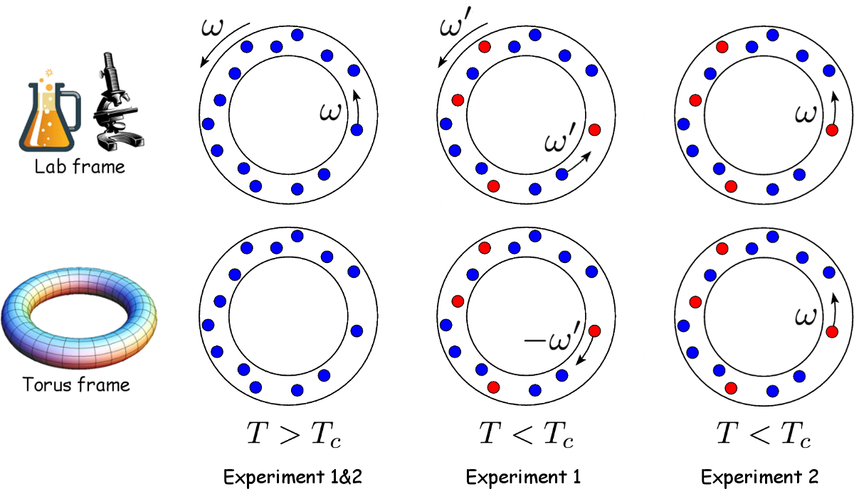
As suggested by LeggetLegget , it is useful to consider two experiments that demonstrate fundamental defining properties of a superfluid (Fig. 1):

• A torus containing liquid Helium ⁴He at temperature $T>T_{c}$ is spun around its axis at low angular frequency, and left in freewheel. Eventually, because of friction, the liquid comes to equilibrium with the moving walls, resulting in a constant angular frequency $\omega$ of the torus. Reducing $T$ below $T_{c}$, an increased angular frequency $\omega^{\prime}>\omega$ of the torus is observed. The conservation of angular momentum implies that a fraction of the liquid, the superfluid, decouples from the rest of the liquid, the normal fluid, and spins at lower (possibly zero) angular frequency. This experimentHess demonstrates the analog of the Meissner effect observed in superconductors.

• Starting with the same setup as above, the torus is spun at high angular frequency. The temperature is then reduced below $T_{c}$ and the torus is brought to rest. Eventually the normal fluid comes to equilibrium with the walls. It can then be verified that the angular momentum of the stationary torus is non-zero (for example, by putting the torus back into freewheel and raising the temperature above $T_{c}$, the torus spontaneously starts to spin). The conservation of angular momentum implies that, while the torus is at rest, the superfluid is still flowing and may continue to do so for a very long time. This experimentWhitmore ; Ekholm demonstrates the analog of persistent dissipationless currents observed in superconductors.

Figure 1: (Color online) Analogs of the Meissner effect (experiment 1) and persistent dissipationless currents (experiment 2) observed in superconductors. At temperature $T>T_{c}$, all fluid is in a normal state (blue spheres) and spins at the angular frequency of the torus. For $T<T_{c}$, a fraction of the fluid becomes superfluid (red spheres) and decouples from the normal fluid.

The outcome of these two experiments can be understood by considering, from the viewpoint of the lab frame, the circulation of the momentum operator $\vec{\mathcal{P}}=-i\hbar\vec{\nabla}$ along a closed loop $\Gamma$ inside the torus around the main axis:

$$\hat{\mathcal{C}}=\oint_{\Gamma}\vec{\mathcal{P}}\cdot\textrm{d}\vec{r}$$ (1)

In the experiment where the torus and the normal fluid are at rest while the superfluid is flowing, the circulation is due to the superfluid only. Suppose that the system is in a state $\big{|}\Psi\big{\rangle}$ that extends over the volume $\Omega$ of the torus. Then the wave function at point $\vec{r}$ can be written as $\langle\vec{r}|\Psi\rangle=\big{|}\langle\vec{r}|\Psi\rangle\big{|}e^{i\phi(\vec{r})}$, where $\phi(\vec{r})$ is the phase, and the expectation value of the superfluid circulation can be expressed as:

$$\big{\langle}\hat{\mathcal{C}}\big{\rangle}_{s} = -i\hbar\big{\langle}\Psi\big{|}\oint_{\Gamma}\vec{\nabla}\cdot\textrm{d}\vec{r}\big{|}\Psi\big{\rangle}$$ (2)

$$= -i\hbar\int_{\Omega}\oint_{\Gamma}\big{\langle}\Psi\big{|}\vec{r}\big{\rangle}\vec{\nabla}\big{\langle}\vec{r}\big{|}\Psi\big{\rangle}\cdot\textrm{d}\vec{r}\>\textrm{d}\Omega$$

$$= -i\hbar\int_{\Omega}\oint_{\Gamma}\big{|}\big{\langle}\Psi\big{|}\vec{r}\big{\rangle}\big{|}\big{(}\vec{\nabla}\big{|}\big{\langle}\vec{r}\big{|}\Psi\big{\rangle}\big{|}\big{)}\cdot\textrm{d}\vec{r}\>\textrm{d}\Omega$$

$$+\hbar\int_{\Omega}\oint_{\Gamma}\big{\langle}\Psi\big{|}\vec{r}\big{\rangle}\big{(}\vec{\nabla}\phi\big{)}\big{\langle}\vec{r}\big{|}\Psi\big{\rangle}\cdot\textrm{d}\vec{r}\>\textrm{d}\Omega$$

Because $\vec{\mathcal{P}}$ is Hermitian, only the real part in (2) can be non-zero. Thus, the circulation depends only on the phase gradient of the wave function and takes the form:

$$\big{\langle}\hat{\mathcal{C}}\big{\rangle}_{s}=\hbar\big{\langle}\oint_{\Gamma}\vec{\nabla}\phi\cdot\textrm{d}\vec{r}\big{\rangle}_{s}$$ (3)

Since the circulation of the phase gradient is along a closed loop, the total variation of the phase must vanish, unless the phase runs over $n$ entire periods of $2\pi$. As a result, the circulation of the superfluid is quantized and can take only the values $\big{\langle}\hat{\mathcal{C}}\big{\rangle}_{s}=2\pi n\hbar$. We note that, from Eq. (3), the existence of a non-zero circulation must be associated with a phase coherence. Expressing the circulation in terms of the velocity $\vec{v}=\vec{\mathcal{P}}/m$, with $m$ the mass of one atom, we find the velocity quantization condition that was first proposed by OnsagerOnsager ,

$$\oint_{\Gamma}\vec{v}_{s}\cdot\textrm{d}\vec{r}=n\kappa_{o},$$ (4)

where $\vec{v}_{s}=\langle\vec{v}\rangle_{s}$ and $\kappa_{o}=\frac{2\pi\hbar}{m}$ is the flux quantum. If the integration loop does not enclose a “hole” (a physical hole like in the torus under consideration, or a vortex), then the path can be shrunk continuously to a point where the circulation vanishes, corresponding to $n=0$. Thus, the only possibility for the circulation to be non-zero is that the loop encloses at least one hole. For a loop that does not include any hole, the application of Stokes’ theorem implies that the superflow is irrotational:

$$\vec{\nabla}\times\vec{v}_{s}=0$$ (5)

We can now make precise what we meant by low and high velocities. When the initial velocity corresponds to less than half a flux quantum (low velocity), the superfluid seeks the nearest velocity satisfying (4) and comes to rest, thus excluding all flux (Meissner effect). When the inital velocity corresponds to more than half a flux quantum (high velocity), the superfluid seeks the nearest velocity satisfying (4) and settles in a persistent dissipationless flow.

The discussion above suggests that transitions between states with different quantum numbers $n$ can be suspected to be associated with vortex formations. The details behind those transitions have been studied numerically for the case of the two-dimensional $XY$ modelBatrouni .

III Thought experiment and definitions of the normal and superfluid densities

III.1 Idealization

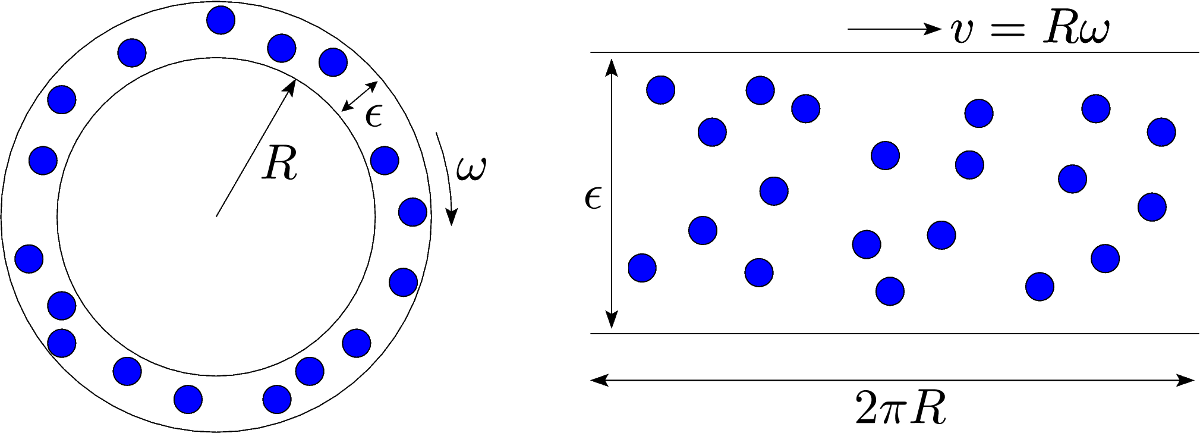
We consider here a thought experiment that idealizes the above real experiment made at low angular frequency. In this experiment, a fluid is enclosed between two $d$-dimensional hypercylinders of radii $R$ and $R+\epsilon$ and infinite mass, rotating with angular frequency $\omega$ (Fig. 2, left). We denote by $\mathcal{F}$ the frame attached to the lab, and by $\mathcal{F}^{\prime}$ the frame attached to the moving walls. In the limit $R\gg\epsilon$, the system becomes equivalent to a fluid enclosed between two hyperplanes of infinite mass separated by a distance $\epsilon$ and moving at constant velocity $v=R\omega$ with respect to $\mathcal{F}$, with a periodicity of $2\pi R$ in the direction of $\vec{v}$ (Fig. 2, right). The outcome of this thought experiment is that, at temperature below $T_{c}$, the superfluid comes to rest with respect to the lab frame, while the normal fluid remains at rest in the frame of the moving walls. Because of the infinite mass of the walls, their velocity with respect to $\mathcal{F}$ does not increase.

Figure 2: (Color online) A fluid is enclosed between two hypercylinders of radii $R$ and $R+\epsilon$ rotating at angular frequency $\omega$ (left). In the limit $R\gg\epsilon$, the system becomes equivalent to one with a fluid enclosed between two hyperplanes moving at velocity $v=R\omega$, and with a periodicity of $2\pi R$ in the direction of $\vec{v}$ (right).

This “thought outcome” does not contradict Galileo’s principle of Relativity. It could be argued that there is no reason for the superfluid to choose to come to rest with respect to $\mathcal{F}$ instead of any other inertial frame. This apparent paradox is resolved by realizing that our description of the system enclosed between two moving hyperplanes is just a limit of the system enclosed between two hypercylinders. Therefore, the frames $\mathcal{F}$ and $\mathcal{F}^{\prime}$ are not equivalent, $\mathcal{F}^{\prime}$ is actually rotating and thus accelerated, and coming to rest with respect to $\mathcal{F}$ is the only way for the superfluid to avoid being accelerated.

III.2 Isotropic case

For a system described by an isotropic Hamiltonian, this thought experiment can be directly generalized to systems with periodicity in all directions: We consider an orthonormal basis $\mathcal{B}=\big{\{}\hat{r}_{1},\cdots,\hat{r}_{d}\big{\}}$ and a system with periodicity $L_{j}$ along each direction $\hat{r}_{j}$ with walls moving at velocity $\vec{v}=(v_{1},\cdots,v_{d})$ with respect to the lab frame $\mathcal{F}$. As the temperature is lowered below $T_{c}$, the superfluid is observed to come to rest with respect to $\mathcal{F}$, while the normal fluid remains at rest with respect to $\mathcal{F}^{\prime}$. Because of the isotropy of the system, this observation must be independent of the direction of $\vec{v}$. As a result, the normal density can be represented by a scalar $\rho_{n}$ and defined as the ratio $\rho_{n}=M_{n}/\Omega$, where $M_{n}$ is the mass of the fluid that comes to rest with respect to the frame of the moving walls $\mathcal{F}^{\prime}$, and $\Omega$ is the volume of the system. In a similar way, the superfluid density can be represented by a scalar $\rho_{s}$ and defined as the ratio $\rho_{s}=M_{s}/\Omega$, where $M_{s}$ is the mass of the fluid that comes to rest with respect to the lab frame $\mathcal{F}$. In the following, we also consider the total mass of the fluid, $M=M_{s}+M_{n}$, and the total density, $\rho=\rho_{s}+\rho_{n}$.

III.3 Anisotropic case

For a system described by an anisotropic Hamiltonian (such as a crystal), the normal and superfluid currents are not necessarily parallel to the velocity $\vec{v}$ of the walls This means that the normal and superfluid densities are second-order tensors, $\rho_{n}^{\zeta\xi}$ and $\rho_{s}^{\zeta\xi}$. Using Einstein’s summation convention, the components of the normal and superfluid current densities $\vec{j}_{n}$ and $\vec{j}_{s}$ take the general form

$$j_{n}^{\zeta}=\rho_{n}^{\zeta\xi}v_{n}^{\xi},$$ (6)

$$j_{s}^{\zeta}=\rho_{s}^{\zeta\xi}v_{s}^{\xi},$$ (7)

where $\vec{v}_{n}$ and $\vec{v}_{s}$ are the normal and superfluid velocities, with $\vec{v}_{n}=\vec{v}$ and $\vec{v}_{s}=0$ in $\mathcal{F}$, and $\vec{v}_{n}=0$ and $\vec{v}_{s}=-\vec{v}$ in $\mathcal{F}^{\prime}$.

IV Calculation of the normal and superfluid densities in continuous space

IV.1 Second quantization preliminaries and notations

We give here a brief reminder of second quantization that is mainly meant to introduce the notation that we use all along this paper. In second quantization, any operator can be expressed as a functional of the creation and annihilation field operators $\hat{\psi}^{\dagger}(\vec{r})$ and $\hat{\psi}(\vec{r})$, with $\vec{r}=(r_{1},\cdots,r_{d})$, which satisfy the relations

$$\big{[}\hat{\psi}(\vec{r}),\hat{\psi}(\vec{r}^{\>\prime})\big{]}_{\zeta}=\big{[}\hat{\psi}^{\dagger}(\vec{r}),\hat{\psi}^{\dagger}(\vec{r}^{\>\prime})\big{]}_{\zeta}=0,$$ (8)

$$\big{[}\hat{\psi}(\vec{r}),\hat{\psi}^{\dagger}(\vec{r}^{\>\prime})\big{]}_{\zeta}=\delta(\vec{r}^{\>\prime}-\vec{r}),$$ (9)

where $[A,B]_{\zeta}\stackrel{{\scriptstyle\textrm{\tiny def}}}{{=}}AB-\zeta BA$ with $\zeta=1$ for bosons and $\zeta=-1$ for fermions, and $\delta(\vec{r}^{\>\prime}-\vec{r})$ is the $d$-dimensional Dirac distribution. The number operator $\hat{\mathcal{N}}$, the position operator $\vec{\mathcal{R}}$, and the momentum operator $\vec{\mathcal{P}}$ take the forms

$$\hat{\mathcal{N}} = \int_{\Omega}\hat{\psi}^{\dagger}(\vec{r})\hat{\psi}(\vec{r})\textrm{d}\Omega,$$ (10)

$$\vec{\mathcal{R}} = \int_{\Omega}\vec{r}\>\hat{\psi}^{\dagger}(\vec{r})\hat{\psi}(\vec{r})\textrm{d}\Omega,$$ (11)

$$\vec{\mathcal{P}} = -i\hbar\int_{\Omega}\hat{\psi}^{\dagger}(\vec{r})\vec{\nabla}_{\vec{r}}\hat{\psi}(\vec{r})\textrm{d}\Omega,$$ (12)

with $\textrm{d}\Omega=\textrm{d}r_{1}\cdots\textrm{d}r_{d}$, and satisfy the commutation relations:

$$\big{[}\mathcal{R}_{\mu},\mathcal{P}_{\nu}\big{]}=i\hbar\delta_{\mu\nu}\hat{\mathcal{N}}$$ (13)

$$\big{[}\vec{\mathcal{R}},\hat{\mathcal{N}}\big{]}=[\vec{\mathcal{P}},\hat{\mathcal{N}}\big{]}=0$$ (14)

From (8), (9), and (11), we can derive additional commulation relations:

$$\big{[}\vec{\mathcal{R}},\hat{\psi}^{\dagger}(\vec{r})]=\vec{r}\>\hat{\psi}^{\dagger}(\vec{r})$$ (15)

$$\big{[}\vec{\mathcal{R}},\hat{\psi}(\vec{r})]=-\vec{r}\>\hat{\psi}(\vec{r})$$ (16)

IV.2 Continuous isotropic case

We consider a $d$-dimensional system of identical particles of mass $m$ in a $L_{1}\times\cdots\times L_{d}$ box with periodic boundary conditions that is moving at low velocity $\vec{v}$ with respect to the lab frame $\mathcal{F}$. In the frame $\mathcal{F}^{\prime}$ of the moving walls the system is at rest. Thus, in this frame, the Hamiltonian is independent of the velocity $\vec{v}$, and is a functional $\Phi$ of the creation and annihilation field operators:

$$\hat{\mathcal{H}}_{o}=\Phi[\hat{\psi}^{\dagger}(\vec{r}),\hat{\psi}(\vec{r})]$$ (17)

Defining the partition function $\mathcal{Z}_{o}=\textrm{Tr }e^{-\beta\hat{\mathcal{H}}_{o}}$ where $\beta$ is the inverse temperature, the average total momentum in $\mathcal{F}^{\prime}$ is given by:

$$\big{\langle}\vec{\mathcal{P}}\big{\rangle}_{\mathcal{F}^{\prime}}=\frac{1}{\mathcal{Z}_{o}}\textrm{Tr }\vec{\mathcal{P}}e^{-\beta\hat{\mathcal{H}}_{o}}$$ (18)

Since $\mathcal{F}$ moves at velocity $-\vec{v}$ with respect to $\mathcal{F}^{\prime}$, the total momentum in the lab frame can be obtained from the above expression by performing an inverse Galilean transformation with velocity $\vec{v}$. For this purpose, it is useful to define the unitary operator:

$$\hat{\mathcal{U}}=e^{-i\frac{m}{\hbar}\vec{v}\cdot\vec{\mathcal{R}}}$$ (19)

By using (13), it is straightforward to check that:

$$\hat{\mathcal{U}}^{\dagger}\vec{\mathcal{P}}\hat{\mathcal{U}}=\vec{\mathcal{P}}-m\vec{v}\hat{\mathcal{N}}$$ (20)

$$\hat{\mathcal{U}}^{\dagger}\vec{\mathcal{R}}\hat{\mathcal{U}}=\vec{\mathcal{R}}$$ (21)

Thus, $\hat{\mathcal{U}}$ is the operator that performs a Galilean transformation (at time $t=0$) with velocity $\vec{v}$, and the total momentum operator in $\mathcal{F}$ is given by the inverse transformation, $\hat{\mathcal{U}}\vec{\mathcal{P}}\hat{\mathcal{U}}^{\dagger}$. Since the density matrix $e^{-\beta\hat{\mathcal{H}}_{o}}/\mathcal{Z}_{o}$ describes probabilities of states, it remains unchanged when going to the lab frame. As a result, the average total momentum in $\mathcal{F}$ takes the form

$$\big{\langle}\vec{\mathcal{P}}\big{\rangle}_{\mathcal{F}} = \frac{1}{\mathcal{Z}_{o}}\textrm{Tr }\hat{\mathcal{U}}\vec{\mathcal{P}}\hat{\mathcal{U}}^{\dagger}e^{-\beta\hat{\mathcal{H}}_{o}}$$ (22)

$$= \frac{1}{\mathcal{Z}_{o}}\textrm{Tr }\vec{\mathcal{P}}e^{-\beta\hat{\mathcal{U}}^{\dagger}\hat{\mathcal{H}}_{o}\hat{\mathcal{U}}}$$

$$= \frac{1}{\mathcal{Z}_{o}}\textrm{Tr }\vec{\mathcal{P}}e^{-\beta\hat{\mathcal{H}}_{\vec{v}}},$$

where we have used the invariance of the trace under cyclic permutations, and we have defined:

$$\hat{\mathcal{H}}_{\vec{v}}=\hat{\mathcal{U}}^{\dagger}\hat{\mathcal{H}}_{o}\hat{\mathcal{U}}$$ (23)

From the correspondence principle, the classical momentum of the fluid must be equal to the quantum average of the momentum operator $\vec{\mathcal{P}}$. Since in $\mathcal{F}$ only the normal fluid with mass $M_{n}=\rho_{n}\Omega$ spins, we have:

$$\rho_{n}\Omega\vec{v}=\frac{1}{\mathcal{Z}_{o}}\textrm{Tr }\vec{\mathcal{P}}e^{-\beta\hat{\mathcal{H}}_{\vec{v}}}$$ (24)

Calculating the divergence of (24) with respect to $\vec{v}$, we get:

$$\vec{\nabla}_{\vec{v}}\cdot(\rho_{n}\Omega\vec{v}) = \Omega\big{(}\vec{\nabla}_{\vec{v}}\rho_{n}\big{)}\cdot\vec{v}+\rho_{n}\Omega d$$ (25)

$$\!\!\!\!\!\!\!\!\!\!\!\!\!\!\!\!\!\!\!\!\!\!\!\!\!\!\!\!\!\!\!\!=-\frac{1}{\mathcal{Z}_{o}}\textrm{Tr }\vec{\mathcal{P}}\cdot\!\!\int_{0}^{\beta}\!\!\!\!e^{-(\beta-\tau)\hat{\mathcal{H}}_{\vec{v}}}\vec{\nabla}_{\vec{v}}\hat{\mathcal{H}}_{\vec{v}}e^{-\tau\hat{\mathcal{H}}_{\vec{v}}}\textrm{d}\tau$$

From (19) and (23), the gradient of $\hat{\mathcal{H}}_{\vec{v}}$ with respect to $\vec{v}$ can be expressed as:

$$\vec{\nabla}_{\vec{v}}\hat{\mathcal{H}}_{\vec{v}}=i\frac{m}{\hbar}\hat{\mathcal{U}}^{\dagger}\big{[}\vec{\mathcal{R}},\hat{\mathcal{H}}_{o}\big{]}\hat{\mathcal{U}}$$ (26)

Injecting (26) in (25) and taking the limit $\vec{v}\to 0$, we get the expression of the normal density:

$$\rho_{n}=-i\frac{m}{\hbar\Omega d}\Big{\langle}\vec{\mathcal{P}}\cdot\int_{0}^{\beta}e^{\tau\hat{\mathcal{H}}_{o}}\big{[}\vec{\mathcal{R}},\hat{\mathcal{H}}_{o}\big{]}e^{-\tau\hat{\mathcal{H}}_{o}}\textrm{d}\tau\Big{\rangle}$$ (27)

From the relation $\rho_{n}+\rho_{s}=\rho$, we deduce the expression of the superfluid density:

$$\rho_{s}=\rho+i\frac{m}{\hbar\Omega d}\Big{\langle}\vec{\mathcal{P}}\cdot\int_{0}^{\beta}e^{\tau\hat{\mathcal{H}}_{o}}\big{[}\vec{\mathcal{R}},\hat{\mathcal{H}}_{o}\big{]}e^{-\tau\hat{\mathcal{H}}_{o}}\textrm{d}\tau\Big{\rangle}$$ (28)

The above expressions of $\rho_{n}$ and $\rho_{s}$ can be evaluated with path-integrals methods, such as the Stochastic Green Function (SGF) algorithmSGF ; DirectedSGF (see paragraphs VII and VIII.3 for concrete examples).

IV.3 Continuous anisotropic case

All equations in the previous subsection can be easily generalized to anisotropic Hamiltonians. By definition, the total momentum in $\mathcal{F}$ is obtained by integrating the normal current density $\vec{j}_{n}$ over the volume $\Omega$. Assuming for the sake of simplicity a uniform current density, we have $\big{\langle}\vec{P}\big{\rangle}_{\mathcal{F}}=\vec{j}_{n}\Omega$. Using (6) in $\mathcal{F}$, the expression of the correspondence principle (24) is generalized as:

$$\rho_{n}^{\zeta\xi}v_{\xi}\Omega=\frac{1}{\mathcal{Z}_{o}}\textrm{Tr }\mathcal{P}_{\zeta}e^{-\beta\hat{\mathcal{H}}_{\vec{v}}}$$ (29)

Calculating the derivative with respect to $v_{\xi}$, and taking the limit $\vec{v}\to 0$, the normal density tensor takes the form:

$$\rho_{n}^{\zeta\xi}=-i\frac{m}{\hbar\Omega}\Big{\langle}\mathcal{P}_{\zeta}\int_{0}^{\beta}e^{\tau\hat{\mathcal{H}}_{o}}\big{[}\mathcal{R}_{\xi},\hat{\mathcal{H}}_{o}\big{]}e^{-\tau\hat{\mathcal{H}}_{o}}\textrm{d}\tau\Big{\rangle}$$ (30)

In order to obtain the superfluid density tensor, it is convenient to consider the total momentum in $\mathcal{F}^{\prime}$. By definition, we have $\big{\langle}\vec{P}\big{\rangle}_{\mathcal{F}^{\prime}}=\vec{j}_{s}\Omega$. Using (7) in $\mathcal{F}^{\prime}$, the correspondence principle implies:

$$-\rho_{s}^{\zeta\xi}v_{\xi}\Omega = \frac{1}{\mathcal{Z}_{o}}\textrm{Tr }\mathcal{P}_{\zeta}e^{-\beta\hat{\mathcal{H}}_{o}}$$ (31)

$$= \frac{1}{\mathcal{Z}_{o}}\textrm{Tr }\hat{\mathcal{U}}^{\dagger}\mathcal{P}_{\zeta}\hat{\mathcal{U}}e^{-\beta\hat{\mathcal{U}}^{\dagger}\hat{\mathcal{H}}_{o}\hat{\mathcal{U}}}$$

$$= \rho_{n}^{\zeta\xi}v_{\xi}\Omega-mv_{\zeta}\big{\langle}\hat{\mathcal{N}}\big{\rangle}$$

Calculating the derivative with respect to $v_{\xi}$, and taking the limit $\vec{v}\to 0$, the superfluid density tensor is obtained from the normal density tensor (30) as:

$$\rho_{s}^{\zeta\xi}=\rho\delta_{\zeta\xi}-\rho_{n}^{\zeta\xi}$$ (32)

IV.4 Relationship between the superfluid density and the free energy

For the simplicity of the following discussion, we consider here only the isotropic case, the generalization to the anisotropic case being straightforward. There exists a particular class of Hamiltonians for which the superfluid density can be directly related to the Laplacian $\Delta_{\vec{v}}$ of the free energy associated to the Hamiltonian $\hat{\mathcal{H}}_{\vec{v}}$,

$$F_{\vec{v}}=-\frac{1}{\beta}\ln\mathcal{Z}_{\vec{v}},$$ (33)

with $\mathcal{Z}_{\vec{v}}=\textrm{Tr }e^{-\beta\hat{\mathcal{H}}_{\vec{v}}}$. This class is defined by Hamiltonians $\hat{\mathcal{H}}_{o}$ for which the commutator with the position operator satisfies:

$$\big{[}\vec{\mathcal{R}},\hat{\mathcal{H}}_{o}\big{]}=i\frac{\hbar}{m}\vec{\mathcal{P}}$$ (34)

The most common example of Hamiltonian that belongs to this class is given by $\hat{\mathcal{H}}_{o}=\hat{\mathcal{T}}+\hat{\mathcal{V}}$, where $\hat{\mathcal{V}}$ is a potential that satisfies $\big{[}\vec{\mathcal{R}},\hat{\mathcal{V}}\big{]}=0$ and $\hat{\mathcal{T}}$ is the kinetic energy:

$$\hat{\mathcal{T}}=-\frac{\hbar^{2}}{2m}\int_{\Omega}\hat{\psi}^{\dagger}(\vec{r})\Delta_{\vec{r}}\hat{\psi}(\vec{r})\textrm{d}\Omega$$ (35)

For any Hamiltonian that satisfies (34), the gradient (26) takes the form

$$\vec{\nabla}_{\vec{v}}\hat{\mathcal{H}}_{\vec{v}}=-\vec{\mathcal{P}}+m\vec{v}\hat{\mathcal{N}},$$ (36)

from which $\vec{\mathcal{P}}$ can be extracted and injected into (24), leading to:

$$\rho_{n}\Omega\vec{v} = -\frac{1}{\mathcal{Z}_{o}}\textrm{Tr }\big{(}\vec{\nabla}_{\vec{v}}\hat{\mathcal{H}}_{\vec{v}}-m\vec{v}\hat{\mathcal{N}}\big{)}e^{-\beta\hat{\mathcal{H}}_{\vec{v}}}$$ (37)

$$= -\frac{\mathcal{Z}_{\vec{v}}}{\mathcal{Z}_{o}}\vec{\nabla}_{\vec{v}}F_{\vec{v}}+\frac{m\vec{v}}{\mathcal{Z}_{o}}\textrm{Tr }\hat{\mathcal{N}}e^{-\beta\hat{\mathcal{H}}_{\vec{v}}}$$

From the divergence of the above expression in the limit $\vec{v}\to 0$, we get for the superfluid density the expression:

$$\rho_{s}=\lim_{\vec{v}\to 0}\frac{1}{\Omega d}\Delta_{\vec{v}}F_{\vec{v}}$$ (38)

At this point, it is useful to determine how the creation and annihilation field operators transform under $\hat{\mathcal{U}}$. Using (15) and (16), we find:

$$\hat{\mathcal{U}}^{\dagger}\hat{\psi}^{\dagger}(\vec{r})\hat{\mathcal{U}}=\hat{\psi}^{\dagger}(\vec{r})e^{i\frac{m}{\hbar}\vec{v}\cdot\vec{r}}$$ (39)

$$\hat{\mathcal{U}}^{\dagger}\hat{\psi}(\vec{r})\hat{\mathcal{U}}=\hat{\psi}(\vec{r})e^{-i\frac{m}{\hbar}\vec{v}\cdot\vec{r}}$$ (40)

As a result, performing a Galilean transformation with velocity $\vec{v}$ is equivalent to applying a phase boost $\varphi(\vec{r})=\frac{m}{\hbar}\vec{v}\cdot\vec{r}$ to the creation and annihilation field operators. This allows us to relate the superfluid density to the response of the free energy to a boundary phase-twistFisher . For this, consider a vector $\vec{L}=n_{1}L_{1}\hat{r}_{1}+\cdots+n_{d}L_{d}\hat{r}_{d}$ where $n_{1},\cdots,n_{d}$ are integers. The phase-twist at the tips of the vector $\vec{L}$ that results from the velocity $\vec{v}$ is $\phi=\frac{m}{\hbar}\vec{v}\cdot\vec{L}$. This allows us to rewrite (38) as:

$$\rho_{s}=\lim_{\phi\to 0}\frac{m^{2}\vec{L}^{2}}{\hbar^{2}\Omega d}\frac{\partial^{2}F_{\phi}}{\partial\phi^{2}}$$ (41)

It is clear that the free energy cannot depend on the sign of the velocity or the phase-twist. This implies:

$$\lim_{\phi\to 0}\frac{\partial^{2}F_{\phi}}{\partial\phi^{2}}=\lim_{\phi\to 0}\frac{1}{\phi}\frac{\partial F_{\phi}}{\partial\phi}$$ (42)

Therefore, the superfluid density is directly related to the response of the free energy to a boundary phase-twistFisher :

$$\rho_{s}=\lim_{\phi\to 0}\frac{m^{2}\vec{L}^{2}}{\hbar^{2}\Omega d\phi}\frac{\partial F_{\phi}}{\partial\phi}$$ (43)

While equations (38), (41), and (43) are well known, it is important to keep in mind that they are valid only for Hamiltonians that satisfy Eq. (34).

IV.5 Relationship between the superfluid density and the winding number

As in the previous subsection, we assume here that the Hamiltonian satisfies the condition (34). In addition, we add the constraint that the Hamiltonian conserves the number of particles, $\big{[}\hat{\mathcal{H}}_{o},\hat{\mathcal{N}}\big{]}=0$. Performing a Taylor expansion and introducing $n$ complete sets of states $\big{|}\Psi_{k}\big{\rangle}$ in the position occupation number representation, the partition function $\mathcal{Z}_{\vec{v}}$ can be written as

$$\mathcal{Z}_{\vec{v}}=\sum_{n\geq 0}\frac{(-\beta)^{n}}{n!}\!\!\!\!\!\!\sum_{\Psi_{1}\cdots\Psi_{n}}\prod_{k=1}^{n}\big{\langle}\Psi_{k+1}\big{|}\hat{\mathcal{H}}_{\vec{v}}\big{|}\Psi_{k}\big{\rangle},$$ (44)

with the convention $\big{|}\Psi_{n+1}\big{\rangle}=\big{|}\Psi_{1}\big{\rangle}$. From (23), we have

$$\prod_{k=1}^{n}\big{\langle}\Psi_{k+1}\big{|}\hat{\mathcal{H}}_{\vec{v}}\big{|}\Psi_{k}\big{\rangle} = \prod_{k=1}^{n}\big{\langle}\Psi_{k+1}\big{|}\hat{\mathcal{H}}_{o}\big{|}\Psi_{k}\big{\rangle}$$ (45)

$$\times e^{i\frac{m}{\hbar}\vec{v}\cdot\sum_{j}L_{j}W_{j}^{\Psi}\hat{r}_{j}},$$

where $W_{j}^{\Psi}$ counts the number of particles that cross the boundaries of the system in the direction $\hat{r}_{j}$ while evolving over the sequence of states $\Psi_{k}$. Therefore the partition function $\mathcal{Z}_{v}$ can be written asBatrouni2

$$\mathcal{Z}_{v} = \sum_{n\geq 0}\sum_{\Psi_{1}\cdots\Psi_{n}}\!\!\!\!\!\!\!\!\!\!\!\!\!\!\underbrace{\frac{(-\beta)^{n}}{n!}\!\prod_{k=1}^{n}\big{\langle}\Psi_{k+1}\big{|}\hat{\mathcal{H}}_{o}\big{|}\Psi_{k}\big{\rangle}}_{\textrm{\tiny Boltzmann weight of a configuration }\Psi_{1}\cdots\Psi_{n}}\!\!\!\!\!\!\!\!\!\!e^{i\frac{m}{\hbar}\vec{v}\cdot\sum_{j}L_{j}W_{j}^{\Psi}\hat{r}_{j}}$$ (46)

$$= \mathcal{Z}_{o}\big{\langle}e^{i\frac{m}{\hbar}\vec{v}\cdot\sum_{j}L_{j}\mathcal{W}_{j}\hat{r}_{j}}\big{\rangle},$$

where $\mathcal{W}_{j}$ are the components of the winding number operator $\vec{\mathcal{W}}$ that take the eigenvalues $W_{j}^{\Psi}$ in a configuration of states $\Psi_{1}\cdots\Psi_{n}$. Injecting (46) into (33), and using (38), the superfluid density becomes directly related to the fluctuations of the winding number:

$$\rho_{s}=\frac{m^{2}}{\hbar^{2}\beta\Omega d}\Big{\langle}\Big{(}\sum_{j}L_{j}\mathcal{W}_{j}\hat{r}_{j}\Big{)}^{2}\Big{\rangle}$$ (47)

For a hypercubic system, $\Omega=L^{d}$, the above expression becomesPollockCeperley :

$$\rho_{s}=\frac{m^{2}L^{2-d}}{\hbar^{2}\beta d}\big{\langle}\vec{\mathcal{W}}^{2}\big{\rangle}$$ (48)

Here too, it is important to keep in mind that while Eq. (48) is well known, it cannot be applied to Hamiltonians that do not satisfy Eq. (34). In addition, the conservation of the number of particles is required for the winding number to be well defined. For Hamiltonians that do not satisfy these conditions, only equations (27) and (28) are valid.

V Calculation of the normal and superfluid densities in discrete space

Determining the expression of the superfluid density in discrete space is not as straightforward as it looks like. In particular, simply replacing the continuous-space operators by their discrete-space equivalents into (28) leads to inconsistencies. The reason is that some of the usual commutation rules between the operators $\hat{\mathcal{N}}$, $\vec{\mathcal{R}}$, $\vec{\mathcal{P}}$, and $\hat{\mathcal{T}}$ are no longer valid when these operators are discretized. It is therefore necessary to proceed carefully with the discretization of space.

V.1 Discretization of space

We start by noticing that (10) represents a dimensionless quantity. This implies that the dimension of the creation and annihilation field operators is the inverse squareroot of a $d$-dimensional volume:

$$\big{[}\hat{\psi}^{\dagger}(\vec{r})\big{]}=\big{[}\hat{\psi}(\vec{r})\big{]}=\mathcal{L}^{-\frac{d}{2}}$$ (49)

Performing for each components of $\vec{r}$ the change of variable $r_{j}=l_{j}y_{j}$, where $l_{j}$ is a positive parameter with the dimension of a length and $y_{j}$ is the new dimensionless variable, we can define the dimensionless creation and annihilation operators

$$a^{\dagger}_{\vec{y}}=\sqrt{l_{1}\cdots l_{d}}\>\hat{\psi}^{\dagger}(l_{1}y_{1},\cdots,l_{d}y_{d}),$$ (50)

$$a_{\vec{y}}=\sqrt{l_{1}\cdots l_{d}}\>\hat{\psi}(l_{1}y_{1},\cdots,l_{d}y_{d}),$$ (51)

which satisfy the same commulation relations as (8) and (9). Using these dimensionless operators, Eq. (10) can be rewritten as

$$\hat{\mathcal{N}}=\int_{\Omega}a^{\dagger}_{\vec{y}}a_{\vec{y}}^{\phantom{\dagger}}\textrm{d}y_{1}\cdots\textrm{d}y_{d},$$ (52)

In the limit $l_{j}\to 0$ the integral becomes independent on the step size $\textrm{d}y_{j}$, which can be chosen to be unity. As a result, the continuous integral can be replaced by a discrete sum over a lattice with constants $l_{1},\cdots,l_{d}$. The commutation relation between the annihilation and the creation operator becomes:

$$\big{[}a_{\vec{y}}^{\phantom{\dagger}},a_{\vec{y}^{\prime}}^{\dagger}\big{]}_{\zeta}=\delta_{\vec{y}\vec{y}^{\>\prime}}$$ (53)

Defining $\hat{n}_{\vec{y}}=a_{\vec{y}}^{\dagger}a_{\vec{y}}^{\phantom{\dagger}}$, the number operator takes the well-known form:

$$\hat{\mathcal{N}}=\sum_{\vec{y}}\hat{n}_{\vec{y}}$$ (54)

Applying the same discretization procedure to the position operator, we get

$$\vec{\mathcal{R}}=\sum_{\vec{y}}\vec{y}_{\vec{l}}\>\hat{n}_{\vec{y}},$$ (55)

with $\vec{y}_{\vec{l}}=(l_{1}y_{1},\cdots,l_{d}y_{d})$. By using for the first-order derivative the symmetrical prescription

$$\frac{\partial}{\partial y_{j}}a_{\vec{y}}=\frac{1}{2}\big{(}a_{\vec{y}+\hat{j}}-a_{\vec{y}-\hat{j}}\big{)},$$ (56)

the discrete momentum operator takes the form

$$\vec{\mathcal{P}}=-i\sqrt{mt_{j}/2}\sum_{\vec{y}}\big{(}a_{\vec{y}}^{\dagger}a_{\vec{y}+\hat{j}}-H.c.\big{)}\hat{j},$$ (57)

where the sum over $j$ is implicit and we have defined $t_{j}=\hbar^{2}/2ml_{j}^{2}$. The above quantity is proportional to what is commonly known as the current density operatorScalapino . In this manuscript we prefer to call it discrete momentum, as it converges to the continuous momentum when the lattice constant goes to zero. It is important to emphasize here that (57) represents a discretization of the real momentum of the system, and that it should not be confused with the crystal quasi-momentum. The importance of this distinction is made clear below. Using for the second-order derivative the symmetrical prescription

$$\frac{\partial^{2}}{\partial y_{\mu}\partial y_{\nu}}a_{\vec{y}} = \frac{1}{2}\big{(}a_{\vec{y}+\hat{\mu}}+a_{\vec{y}-\hat{\mu}}+a_{\vec{y}+\hat{\nu}}+a_{\vec{y}-\hat{\nu}}$$ (58)

$$-a_{\vec{y}+\hat{\mu}-\hat{\nu}}-a_{\vec{y}-\hat{\mu}+\hat{\nu}}-2a_{\vec{y}}\big{)},$$

the discrete kinetic operator takes the form $\hat{\mathcal{T}}=\sum_{j}\hat{\mathcal{T}}_{j}$, where $\hat{\mathcal{T}}_{j}$ is given by:

$$\hat{\mathcal{T}}_{j}=-t_{j}\sum_{\vec{y}}\big{(}a_{\vec{y}}^{\dagger}a_{\vec{y}+\hat{j}}+H.c.\big{)}+2t_{j}\hat{\mathcal{N}}$$ (59)

Note that the second term in (59) is usually dismissed because it only gives rise to a shift of the chemical potential and does not change the physics. In our case, we explicitly take it into account in order to ease the connection with the continuous case. With these discrete operators, it is easy to check that the commutator (13) becomes:

$$\big{[}\mathcal{R}_{\mu},\mathcal{P}_{\nu}\big{]}=i\hbar\delta_{\mu\nu}\Big{(}\hat{\mathcal{N}}-\frac{1}{2t_{\mu}}\hat{\mathcal{T}}_{\mu}\Big{)}$$ (60)

As a result, as opposed to the continuous case, the discrete position operator $\vec{\mathcal{R}}$ is not the generator of infinitesimal translations in real momentum space. It actually translates the quasi-momentum only. Therefore the unitary operator $\hat{\mathcal{U}}=e^{-i\frac{m}{\hbar}\vec{v}\cdot\vec{\mathcal{R}}}$ is no longer the operator that performs a Galilean transformation with velocity $\vec{v}$. This implies that Eq. (22) and (29) are not applicable in the discrete case and need to be modified. To this end, it is useful to determine how the real momentum $\vec{\mathcal{P}}$ transforms under $\hat{\mathcal{U}}$ at first order in $\vec{v}$. Using (60) we find:

$$\hat{\mathcal{U}}\vec{\mathcal{P}}\hat{\mathcal{U}}^{\dagger}=\vec{\mathcal{P}}+m\vec{v}\hat{\mathcal{N}}-\frac{m}{2}\sum_{j}\frac{v_{j}}{t_{j}}\hat{j}\hat{\mathcal{T}}_{j}+\vec{\mathcal{O}}(\vec{v}^{2})$$ (61)

This implies that new terms proportional to $\big{\langle}\hat{\mathcal{T}}_{j}\big{\rangle}$ must be introduced when discretizing (22) or (29).

V.2 Discrete isotropic case

Using (61) with $t_{j}=t$, (22) becomes:

$$\big{\langle}\vec{\mathcal{P}}\big{\rangle}_{\mathcal{F}}=\frac{1}{\mathcal{Z}_{o}}\textrm{Tr }\vec{\mathcal{P}}e^{-\beta\hat{\mathcal{H}}_{\vec{v}}}+\frac{m}{2t}\sum_{j}v_{j}\hat{j}\big{\langle}\hat{\mathcal{T}}_{j}\big{\rangle}+\vec{\mathcal{O}}(\vec{v}^{2})$$

As before, the correspondence principle requires the above quantum average of the momentum to be equal to the classical momentum, which in $\mathcal{F}$ is due to the normal fluid only, $\rho_{n}\Omega\vec{v}$. Calculating the divergence of this equality and taking the limit $\vec{v}\to 0$, we deduce the expression of the normal density:

$$\rho_{n}=\frac{m}{2td\Omega}\big{\langle}\hat{\mathcal{T}}\big{\rangle}-i\frac{m}{\hbar\Omega d}\Big{\langle}\vec{\mathcal{P}}\cdot\int_{0}^{\beta}e^{\tau\hat{\mathcal{H}}_{o}}\big{[}\vec{\mathcal{R}},\hat{\mathcal{H}}_{o}\big{]}e^{-\tau\hat{\mathcal{H}}_{o}}\textrm{d}\tau\Big{\rangle}$$ (62)

As a result, the expression of the superfluid density is:

$$\rho_{s} = \rho-\frac{m}{2td\Omega}\big{\langle}\hat{\mathcal{T}}\big{\rangle}$$ (63)

$$+i\frac{m}{\hbar\Omega d}\Big{\langle}\vec{\mathcal{P}}\cdot\int_{0}^{\beta}e^{\tau\hat{\mathcal{H}}_{o}}\big{[}\vec{\mathcal{R}},\hat{\mathcal{H}}_{o}\big{]}e^{-\tau\hat{\mathcal{H}}_{o}}\textrm{d}\tau\Big{\rangle}$$

Comparing (28) and (63), we see that not only have the continuous-space operators been replaced by their discrete-space equivalents, but a new term proportional to the kinetic energy also appeared. It can be checked that (62) and (63) converge respectively to (27) and (28) in the limit $l\to 0$. The consistency of Eq.(63) can also be checked by verifying that it reduces to Eq.(13) of Ref.Scalapino when applied to the particular case discussed there.

V.3 Discrete anisotropic case

Using (61), (29) becomes:

$$\rho_{n}^{\zeta\xi}v_{\xi}\Omega=\frac{1}{\mathcal{Z}_{o}}\textrm{Tr }\mathcal{P}_{\zeta}e^{-\beta\hat{\mathcal{H}}_{\vec{v}}}+\frac{mv_{\zeta}}{2t_{\zeta}}\big{\langle}\hat{\mathcal{T}}_{\zeta}\big{\rangle}+\mathcal{O}(\vec{v}^{2})$$ (64)

Calculating the derivative with respect to $v_{\xi}$ in the limit $\vec{v}\to 0$, we get the normal density tensor:

$$\rho_{n}^{\zeta\xi} = \frac{m}{2\Omega t_{\zeta}}\delta_{\zeta\xi}\big{\langle}\hat{\mathcal{T}}_{\zeta}\big{\rangle}$$ (65)

$$-i\frac{m}{\hbar\Omega}\Big{\langle}\mathcal{P}_{\zeta}\int_{0}^{\beta}e^{\tau\hat{\mathcal{H}}_{o}}\big{[}\mathcal{R}_{\xi},\hat{\mathcal{H}}_{o}\big{]}e^{-\tau\hat{\mathcal{H}}_{o}}\textrm{d}\tau\Big{\rangle}$$

As before, the superfluid density tensor is obtained as a function of the normal density tensor (32).

V.4 The superfluid density as a function of the free energy and the winding number

For simplicity, we consider in the remaining of this section only the isotropic case, the generalization to the anisotropic case being straightforward. As for the continuous-space case, the superfluid density can be related to the free energy if the Hamiltonian satisfies $\big{[}\vec{\mathcal{R}},\hat{\mathcal{H}}_{o}\big{]}=i\frac{\hbar}{m}\vec{\mathcal{P}}$. In this case, the gradient $\vec{\nabla}\hat{\mathcal{H}}_{\vec{v}}=-\hat{\mathcal{U}}^{\dagger}\vec{\mathcal{P}}\hat{\mathcal{U}}$ is given by the opposite of the inverse transfomation of (61):

$$\vec{\nabla}\hat{\mathcal{H}}_{\vec{v}}=-\vec{\mathcal{P}}+m\vec{v}\hat{\mathcal{N}}-\frac{m}{2t}\sum_{j}v_{j}\hat{j}\hat{\mathcal{T}}_{j}+\vec{\mathcal{O}}(\vec{v}^{2})$$ (66)

Extracting $\vec{\mathcal{P}}$ from the above expression and injecting it into (V.2), we get:

$$\big{\langle}\vec{\mathcal{P}}\big{\rangle}_{\mathcal{F}} = -\frac{\mathcal{Z}_{\vec{v}}}{\mathcal{Z}_{o}}\vec{\nabla}F_{\vec{v}}+m\vec{v}\frac{1}{\mathcal{Z}_{o}}\textrm{Tr }\hat{\mathcal{N}}e^{-\beta\hat{\mathcal{H}}_{\vec{v}}}$$ (67)

$$-\frac{m}{2t}\sum_{j}v_{j}\hat{j}\frac{1}{\mathcal{Z}_{o}}\textrm{Tr }\hat{\mathcal{T}}_{j}e^{-\beta\hat{\mathcal{H}}_{\vec{v}}}$$

$$+\frac{m}{2t}\sum_{j}v_{j}\hat{j}\big{\langle}\hat{\mathcal{T}}_{j}\big{\rangle}+\vec{\mathcal{O}}(\vec{v}^{2})$$

Calculating the divergence of (67) and taking the limit $\vec{v}\to 0$, the terms in $\hat{\mathcal{T}}_{j}$ cancel out. Thus, the expression of $\rho_{s}$ as a function of the free energy in discrete space is the same as in continuous space (38), and so are the expressions of $\rho_{s}$ as the response of the free energy to a phase boost (43), and as a function of the winding number (47).

V.5 Dimensionless superfluid density

For lattice systems, it is common to work with the dimensionless superfluid density $\tilde{\rho}_{s}$, defined as the superfluid fraction $\eta_{s}=\rho_{s}/\rho$ times the dimensionless density $\tilde{\rho}=\langle\hat{\mathcal{N}}\rangle/S_{\textrm{\tiny tot}}$, where $S_{\textrm{\tiny tot}}=S_{1}\times\cdots\times S_{d}$ is the total number of lattice sites. This can be written as:

$$\tilde{\rho}_{s}=\frac{\rho_{s}\Omega}{mS_{\textrm{\tiny tot}}}$$ (68)

Injecting (63) into (68), the dimensionless superfluid density takes the general form:

$$\tilde{\rho}_{s} = \tilde{\rho}-\frac{1}{2tdS_{\textrm{\tiny tot}}}\big{\langle}\hat{\mathcal{T}}\big{\rangle}$$ (69)

$$+i\frac{1}{\hbar dS_{\textrm{\tiny tot}}}\Big{\langle}\vec{\mathcal{P}}\cdot\int_{0}^{\beta}e^{\tau\hat{\mathcal{H}}_{o}}\big{[}\vec{\mathcal{R}},\hat{\mathcal{H}}_{o}\big{]}e^{-\tau\hat{\mathcal{H}}_{o}}\textrm{d}\tau\Big{\rangle}$$

VI Lattices with non-orthonormal primitive vectors

In order to obtain the correct expressions of the superfluid density in lattices with non-cubic primitive cells, it is necessary to perform a careful change of basis when discretizing space.

VI.1 Change of basis

We consider an orthonormal basis, $\mathcal{B}_{r}=\{\hat{r}_{1},\cdots,\hat{r}_{d}\}$, and a transformation $\mathcal{A}$ that changes $\mathcal{B}_{r}$ into a general basis, $\mathcal{B}_{q}=\{\vec{q}_{1},\cdots,\vec{q}_{d}\}$. We denote by $A$ the matrix representation of $\mathcal{A}$ in the basis $\mathcal{B}_{r}$. Position vectors are contravariant, thus their coordinates $(q^{1},\cdots,q^{d})$ in $\mathcal{B}_{q}$ are obtained from their coordinates $(r^{1},\cdots,r^{d})$ in $\mathcal{B}_{r}$ by the inverse transformation,

$$q^{i}=A^{-1}_{ij}r^{j},$$ (70)

where we have used Einstein’s summation convention. On the contrary, the derivatives with respect to the coordinates are covariant,

$$\frac{\partial}{\partial q_{j}}=A_{ij}\frac{\partial}{\partial r_{i}},$$ (71)

thus the Laplacian in the basis $\mathcal{B}_{q}$ takes the form:

$$\Delta_{\vec{q}}=A^{-1}_{ik}A^{-1}_{jk}\frac{\partial^{2}}{\partial q_{i}\partial q_{j}}$$ (72)

Defining the metric tensor $g_{\mu\nu}=\vec{q}_{\mu}\cdot\vec{q}_{\nu}$, the dot-product in the basis $\mathcal{B}_{q}$ of two vectors $\vec{u}=(u^{1},\cdots,u^{d})$ and $\vec{v}=(v^{1},\cdots,v^{d})$ takes the form:

$$\vec{u}\cdot\vec{v}=g_{\mu\nu}u^{\mu}v^{\nu}$$ (73)

VI.2 Discretization of space in non-orthonormal coordinates

For the sake of simplicity, we assume in the remainder of this section that the Hamiltonian is of the form $\hat{\mathcal{H}}_{o}=\hat{\mathcal{T}}+\hat{\mathcal{V}}$, so the relationship between the superfluid density and the winding number applies. A condition for the discretization to be valid is that the discretized Hamiltonian should reproduce quantitatively the same physics as its continuous space analog when the lattice constants go to zero. By performing the change of variables (70), the continuous-space kinetic operator (35) can be rewritten as

$$\hat{\mathcal{T}}=-\frac{\hbar^{2}|J|A^{-1}_{ik}A^{-1}_{jk}}{2m}\int_{\Omega}\!\!\hat{\psi}^{\dagger}(\vec{q})\frac{\partial^{2}}{\partial q_{i}\partial q_{j}}\hat{\psi}(\vec{q})\textrm{d}Q,$$ (74)

where $|J|$ is the Jacobian determinant,

$$|J|=\bigg{|}\frac{\partial(r^{1},\cdots,r^{d})}{\partial(q^{1},\cdots,q^{d})}\bigg{|},$$ (75)

and $\textrm{d}Q=\textrm{d}q_{1}\cdots\textrm{d}q_{d}$. Performing a second change of variables for each coordinates, $q_{j}=l_{j}y_{j}$, where $l_{j}$ has the dimension of a length and $y_{j}$ is the new dimensionless variable, the kinetic operator becomes

$$\hat{\mathcal{T}}=-\frac{\hbar^{2}|J|A^{-1}_{ik}A^{-1}_{jk}}{2ml_{i}l_{j}}\int_{\Omega}\!\!a^{\dagger}_{\vec{y}}\frac{\partial^{2}}{\partial y_{i}\partial y_{j}}a_{\vec{y}}^{\phantom{\dagger}}\>\textrm{d}y_{1}\cdots\textrm{d}y_{d},$$ (76)

where we have used the previously defined dimensionless creation and annihilation operators, (50) and (51). As before, in the limit $l_{j}\to 0$, the integral becomes independent of the step size $\textrm{d}y_{j}$, which can be chosen as unity. In this case, the integral becomes discrete, $l_{j}$ becomes the lattice constant in the $\vec{q}_{j}$ direction, and the kinetic operator takes the form:

$$\hat{\mathcal{T}}=-\frac{\hbar^{2}|J|A^{-1}_{ik}A^{-1}_{jk}}{2ml_{i}l_{j}}\sum_{\vec{y}\in\Omega}a^{\dagger}_{\vec{y}}\frac{\partial^{2}}{\partial y_{i}\partial y_{j}}a_{\vec{y}}^{\phantom{\dagger}}$$ (77)

It is important to keep in mind that the volume $\Omega$ is a hyperrectangle. However, if the basis $\mathcal{B}_{q}$ is not orthogonal, summing over a hyperparallelepiped turns out to be more convenient. As a result, instead of a hyperrectangle of volume $\Omega=\prod_{j}L_{j}$, we consider a hyperparallelepiped of volume $\tilde{\Omega}=|J|\prod_{j}L_{j}$. Since the volume $\tilde{\Omega}$ is scaled by a factor $|J|$ with respect to $\Omega$, the same energy can be recovered by multiplying it by the inverse factor. Therefore, the Jacobian determinant disappears and the kinetic operator is equivalent to

$$\hat{\mathcal{T}}=-\frac{\hbar^{2}A^{-1}_{ik}A^{-1}_{jk}}{2ml_{i}l_{j}}\sum_{\vec{y}\in\tilde{\Omega}}a^{\dagger}_{\vec{y}}\frac{\partial^{2}}{\partial y_{i}\partial y_{j}}a_{\vec{y}}^{\phantom{\dagger}},$$ (78)

where the summation is over all vectors $\vec{y}$ in the volume $\tilde{\Omega}$ with the components $y_{j}$ varying over $S_{j}=L_{j}/l_{j}$ lattice sites. We can use for the second-order derivative the previous symmetrical prescription (58). The discretization of the potential term $\hat{\mathcal{V}}$ can be done in a similar way, and does not affect the following conclusions.

VI.3 Application to Bravais lattices

We give here some examples of application of the above discretization to some common Bravais lattices, and we emphasize the differences between our expressions for the superfluid density and the expressions that are usually improperly used. For simplicity, we consider here only isotropic cases.

VI.3.1 Hypercubic lattice

In the case of a hypercubic lattice with $S_{1}\times\cdots\times S_{d}$ sites, the basis of the primitive cell is orthogonal, and the lattice constants $l_{j}$ are all equal to the same value $l$. Using the identity transformation for $\mathcal{A}$ and defining $t=\frac{\hbar^{2}}{2ml^{2}}$, Eq. (78) leads to the previous discrete form of the kinetic energy:

$$\hat{\mathcal{T}}=-t\sum_{\langle p,q\rangle}\big{(}a_{p}^{\dagger}a_{q}^{\phantom{\dagger}}+H.c.\big{)}+2td\hat{\mathcal{N}}$$ (79)

In this simple case, the metric tensor $g_{\mu\nu}$ is just the identity, and combining (48) and (68) leads to

$$\tilde{\rho}_{s}=\frac{S^{2-d}}{2t\beta d}\langle\mathcal{W}_{1}^{2}+\cdots+\mathcal{W}_{d}^{2}\rangle,$$ (80)

where we have assumed the same number of lattice sites $S_{j}=S$ in each of the primitive directions. For this case, we recover the well-known expression. A common mistake arises when applying (80) to non-cubic lattice geometries, as we show below.

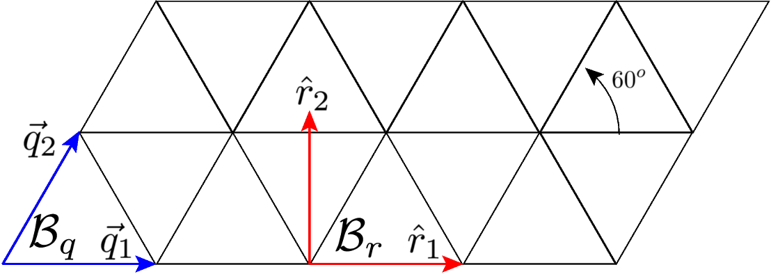
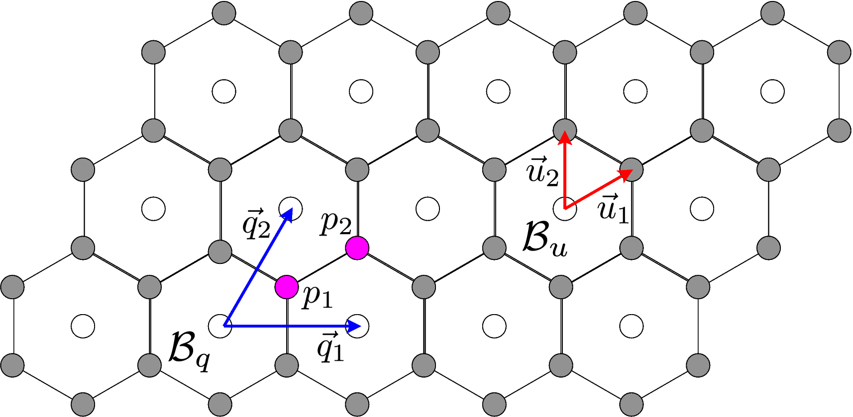
VI.3.2 Triangular lattice

We address here the case of a $S\times S$ triangular lattice (Fig. 3). The transformation matrix $A$ that changes the orthonormal basis $\mathcal{B}_{r}=\{\hat{r}_{1},\hat{r}_{2}\}$ into the basis $\mathcal{B}_{q}=\{\vec{q}_{1},\vec{q}_{2}\}$ and the metric tensor $g_{\mu,\nu}$ are given by:

$$A=\left(\begin{array}[]{cc}1&1/2\\ 0&\sqrt{3}/2\end{array}\right),\quad g=\left(\begin{array}[]{cc}1&1/2\\ 1/2&1\end{array}\right)$$ (81)

Figure 3: (Color online) Triangular lattice. The basis $\mathcal{B}_{r}$ is changed to $\mathcal{B}_{q}$ by the transformation (81).

With this transformation, Eq. (78) becomes

$$\hat{\mathcal{T}}=-t^{\prime}\sum_{\langle p,q\rangle}\big{(}a_{p}^{\dagger}a_{q}^{\phantom{\dagger}}+H.c.\big{)}+6t^{\prime}\hat{\mathcal{N}},$$ (82)

with the energy scale $t^{\prime}=\frac{\hbar^{2}}{3ml^{2}}$. As a result, using (73) for the square of the winding number operator, the dimensionless superfluid density is:

$$\tilde{\rho}_{s}=\frac{1}{6t^{\prime}\beta}\langle\mathcal{W}_{1}^{2}+\mathcal{W}_{2}^{2}+\mathcal{W}_{1}\mathcal{W}_{2}\rangle$$ (83)

The above expression computed with the energy scale $t^{\prime}=1$ differs significantly from the quantity (80) that is usually improperly applied with $t=1$. Doing so not only introduces an energy scale mismatch between the simulated Hamiltonian and the computed superfluid density, but some winding correlations are missed too.

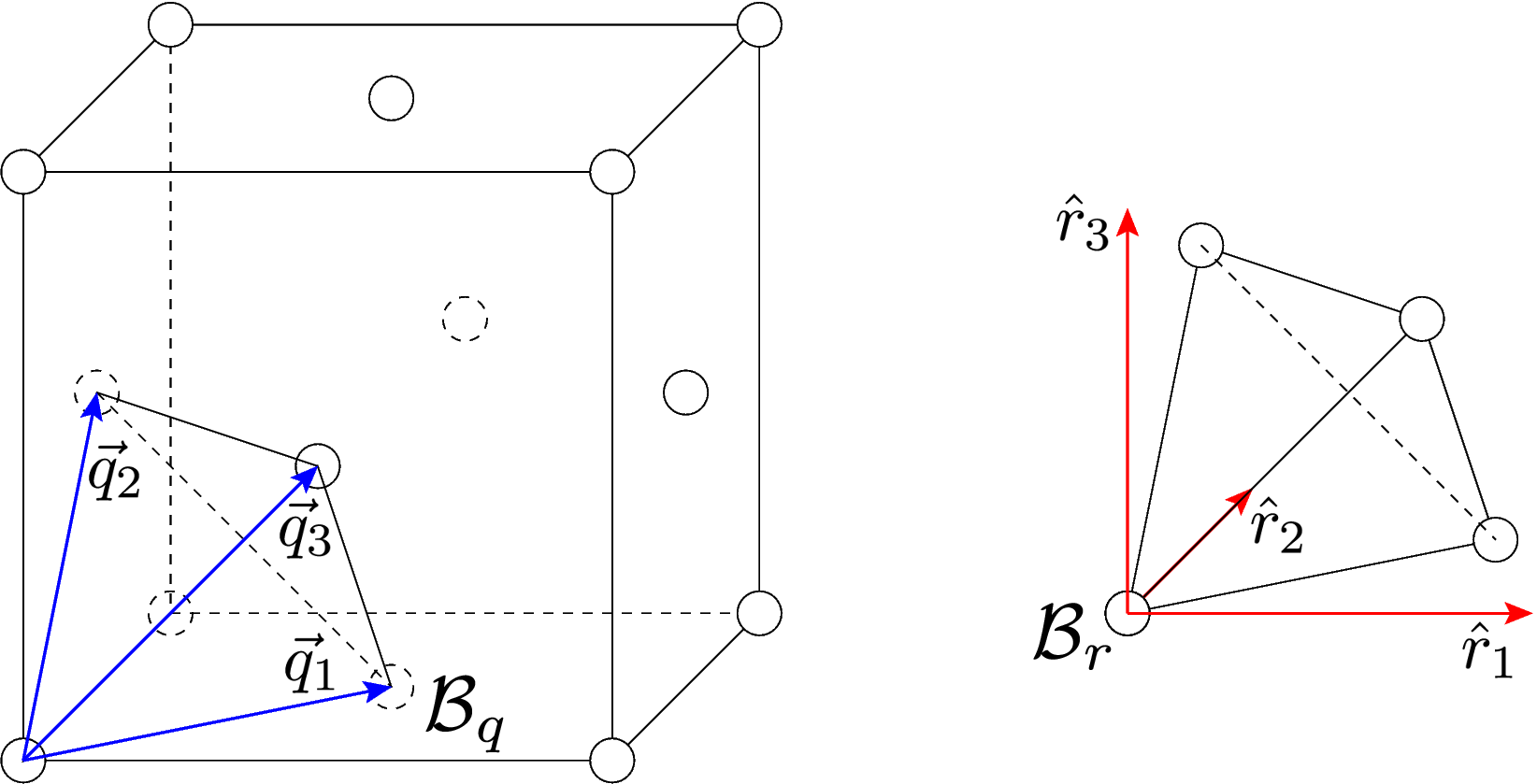
VI.3.3 Face-centered cubic lattice

The transformation matrix $A$ and the metric tensor $g_{\mu,\nu}$ associated to the primitive cell of a face-centered cubic lattice (Fig. 4) are given by:

$$A=\frac{1}{\sqrt{2}}\left(\begin{array}[]{ccc}1&0&1\\ 1&1&0\\ 0&1&1\end{array}\right),\quad g=\left(\begin{array}[]{ccc}1&1/2&1/2\\ 1/2&1&1/2\\ 1/2&1/2&1\end{array}\right)$$ (84)

Figure 4: (Color online) Face-centered cubic lattice. The basis $\mathcal{B}_{r}$ is changed to $\mathcal{B}_{q}$ by the transformation (84).

With this transformation, Eq. (78) becomes

$$\hat{\mathcal{T}}=-t^{\prime\prime}\sum_{\langle p,q\rangle}\big{(}a_{p}^{\dagger}a_{q}^{\phantom{\dagger}}+H.c.\big{)}+12t^{\prime\prime}\hat{\mathcal{N}},$$ (85)

with the energy scale $t^{\prime\prime}=\frac{\hbar^{2}}{4ml^{2}}$. Thus, for a $S\times S\times S$ lattice, the dimensionless superfluid density takes the form:

$$\tilde{\rho}_{s}=\frac{\langle\mathcal{W}_{1}^{2}+\mathcal{W}_{2}^{2}+\mathcal{W}_{3}^{2}+\mathcal{W}_{1}\mathcal{W}_{2}+\mathcal{W}_{2}\mathcal{W}_{3}+\mathcal{W}_{3}\mathcal{W}_{1}\rangle}{12t^{\prime\prime}\beta S}$$ (86)

Once again, the above expression computed with the energy scale $t^{\prime\prime}=1$ differs significantly from the quantity (80) that is usually improperly applied with $t=1$.

VI.4 Application to non-Bravais lattices

A non-Bravais lattice can be described as a basis of points that is reproduced at each point of an underlying Bravais lattice. Another possible description is to consider it as a Bravais lattice with smaller lattice constants and missing points. The advantage of this latter description is that we already know how to discretize continuous space and obtain a Bravais lattice with the associated expression of the superfluid density. By adding to the Hamiltonian an infinite potential at the locations of the missing points, we can prevent the particles from occupying those positions and generate the corresponding non-Bravais lattice. This mathematical “trick” allows us to determine the expression of the superfluid density.

VI.4.1 Honeycomb lattice

A honeycomb lattice (Fig. 5) is usually seen as a two-point basis $(p_{1},p_{2})$ that is reproduced at each point of a triangular lattice generated by a basis $\mathcal{B}_{q}$. In our case, it is more convenient to describe it as a triangular lattice generated by a second basis $\mathcal{B}_{u}$, to which we remove all points generated by the basis $\mathcal{B}_{q}$.

Figure 5: (Color online) A honeycomb lattice can be described as a two-point basis $(p_{1},p_{2})$ that is reproduced at each point of a triangular lattice generated by a basis $\mathcal{B}_{q}$, or as a triangular lattice generated by a basis $\mathcal{B}_{u}$ to which all points generated by the basis $\mathcal{B}_{q}$ are removed.

At this point, it is useful to consider the Hamiltonian $\hat{\mathcal{H}}=\hat{\mathcal{T}}+\hat{\mathcal{V}}$ with $\hat{\mathcal{T}}$ given by (35) and $\hat{\mathcal{V}}$ by

$$\hat{\mathcal{V}}=\int_{\Omega}\hat{\psi}^{\dagger}(\vec{r})V(\vec{r})\hat{\psi}(\vec{r})\textrm{d}\Omega,$$ (87)

with

$$V(\vec{r})=Uh^{2}\sum_{j_{1},j_{2}}\delta(\vec{r}-j_{1}\vec{q}_{1}-j_{2}\vec{q}_{2}),$$ (88)

where $U$ is a parameter with the dimension of an energy and $h=||\vec{q}_{1}||=||\vec{q}_{2}||$. Injecting (88) into (87) and using the previously defined dimensionless creation and annihilation operators (50) and (51), the potential becomes:

$$\hat{\mathcal{V}}=U\sum_{j_{1},j_{2}}\hat{n}_{j_{1}\vec{q}_{1}+j_{2}\vec{q}_{2}}$$ (89)

By discretizing $\hat{\mathcal{T}}$ with the transformation that changes an orthogonal basis into the basis $\mathcal{B}_{u}$ and defining $l=||\vec{u}_{1}||=||\vec{u}_{2}||$, the Hamiltonian becomes

$$\hat{\mathcal{H}} = -t^{\prime}\sum_{\langle p,q\rangle}(a_{p}^{\dagger}a_{q}^{\phantom{\dagger}}+H.c.\big{)}+6t^{\prime}\hat{\mathcal{N}}$$ (90)

$$+U\sum_{p\in\mathcal{B}_{q}}\hat{n}_{p}$$

where the sum $\sum_{\langle p,q\rangle}$ is over all distinct pairs of first neighboring sites of the triangular lattice generated by $\mathcal{B}_{u}$, and the sum $\sum_{p\in\mathcal{B}_{q}}$ is over all sites generated by $\mathcal{B}_{q}$. Since the Hamiltonian $\hat{\mathcal{H}}$ satisfies the condition (34), the corresponding superfluid density is given by (83), and this result applies for any value of the parameter $U$. In particular, it applies in the limit $U\to\infty$ where the Hamiltonian becomes equivalent to

$$\hat{\mathcal{H}}=-t^{\prime}\sum_{\langle p,q\rangle-{\mathcal{B}_{q}}}(a_{p}^{\dagger}a_{q}^{\phantom{\dagger}}+H.c.\big{)}+6t^{\prime}\hat{\mathcal{N}},$$ (91)

where the notation $\langle p,q\rangle-{\mathcal{B}_{q}}$ indicates that the points generated by $\mathcal{B}_{q}$ are removed. As a result, the above Hamiltonian describes particles on a honeycomb lattice, and the expression of the superfluid density is the same as for a triangular lattice and given by (83).

VI.4.2 Kagome lattice

A kagome lattice (Fig. 6) is formed by corner-sharing triangles, and is usually seen as a three-point basis $(p_{1},p_{2},p_{3})$ that is reproduced at each point of a triangular lattice generated by a basis $\mathcal{B}_{q}$. Here again, it is more convenient to describe it as a triangular lattice generated by a second basis $\mathcal{B}_{u}$, to which we remove all points generated by the basis $\mathcal{B}_{q}$.

Figure 6: (Color online) A kagome lattice can be described as a three-point basis $(p_{1},p_{2},p_{3})$ that is reproduced at each point of a triangular lattice generated by a basis $\mathcal{B}_{q}$, or as a triangular lattice generated by a basis $\mathcal{B}_{u}$ to which all points generated by the basis $\mathcal{B}_{q}$ are removed.

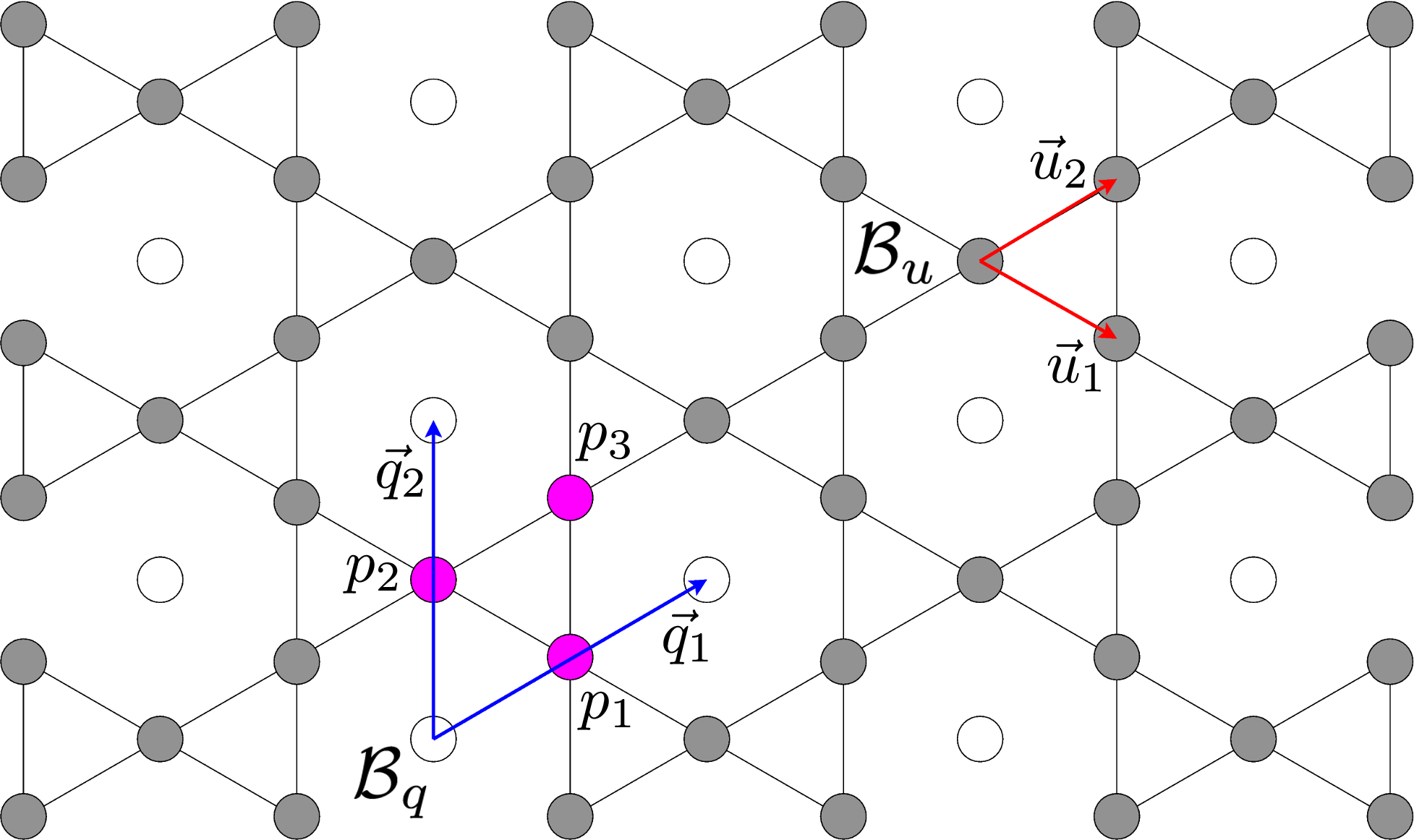
Therefore, the same reasoning as for the honeycomb lattice can be applied, and we conclude that the expression of the superfluid density is given by that of a triangular lattice (83).

VI.4.3 Pyrochlore lattice

A pyrochlore lattice (Fig. 7) is formed by corner-sharing tetrahedrons, and is usually seen as a four-point basis $(p_{1},p_{2},p_{3},p_{4})$ that is reproduced at each point of a face-centered cubic lattice generated by a basis $\mathcal{B}_{q}$. In a way similar to the honeycomb and kagome lattices, it is more convenient to describe it as a face-centered cubic lattice generated by a second basis $\mathcal{B}_{u}$, to which we remove all points generated by the basis $\mathcal{B}_{q}$.

Figure 7: (Color online) A pyrochlore lattice can be described as a four-point basis $(p_{1},p_{2},p_{3},p_{4})$ that is reproduced at each point of a face-centered cubic lattice generated by a basis $\mathcal{B}_{q}$, or as a face-centered cubic lattice generated by a basis $\mathcal{B}_{u}$ to which the points generated by the basis $\mathcal{B}_{q}$ are removed.

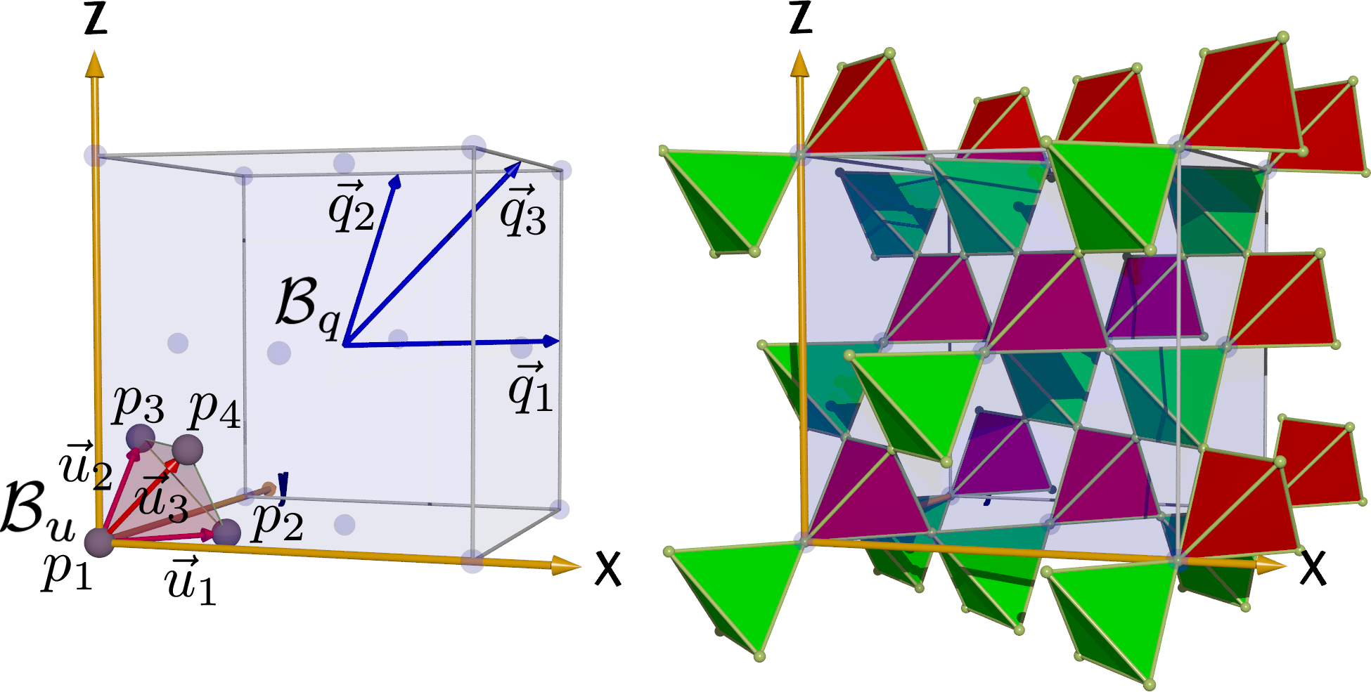
As before, the same reasoning as for the honeycomb and kagome lattices can be applied, and we conclude that the expression of the superfluid density is given by that of a face-centered cubic lattice (86).

VI.5 Consistency check

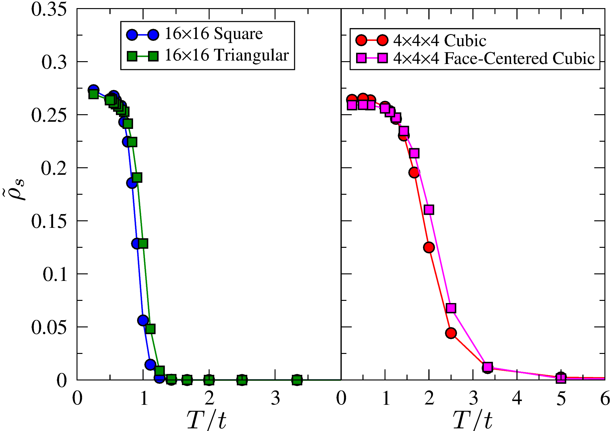
In this subsection, we make a consistency check that illustrates the correctness of our expressions of the superfluid density for the hypercubic (80), triangular (83), and face-centered cubic (86) lattices. Since the kinetic term of the triangular lattice (82) and the kinetic term of the face-centered cubic (85) lattice correspond to the discretization of the continuous kinetic term (35) with $d=2$ and $d=3$, respectively, they should give exactly the same superfluid density as the kinetic term of the hypercubic lattice (79) with the corresponding dimensionality.

In order to check this, we made use of the Stochastic Green FunctionSGF (SGF) algorithm with directed updatesDirectedSGF , and performed quantum Monte Carlo simulations of the kinetic term for hard-core bosons at half-filling. The results are shown in Fig. 8. The superfluid density obtained for a $16\times 16$ triangular lattice with $t^{\prime}=1$ is in agreement with the superfluid density obtained for a $16\times 16$ square lattice with $t=1$, as a function of temperature $T$, the small differences being due to finite-size effects. We get the same agreement between the superfluid density obtained for a $4\times 4\times 4$ face-centered cubic lattice with $t^{\prime\prime}=1$ and the superfluid density obtained for a $4\times 4\times 4$ cubic lattice with $t=1$.

Figure 8: (Color online) The dimensionless superfluid density $\tilde{\rho}_{s}$ of hard-core bosons as a function of temperature $T/t$ at half-filling, for different lattice geometries. The values obtained for a triangular lattice agree with the values obtained for a square lattice, the small differences being due to finite-size effects. In the same way, the values obtained for a face-centered cubic lattice agree with the values obtained for a cubic lattice. The errorbars are smaller than the symbols’ size.

VII Lattice Hamiltonian with hopping between second neighbors

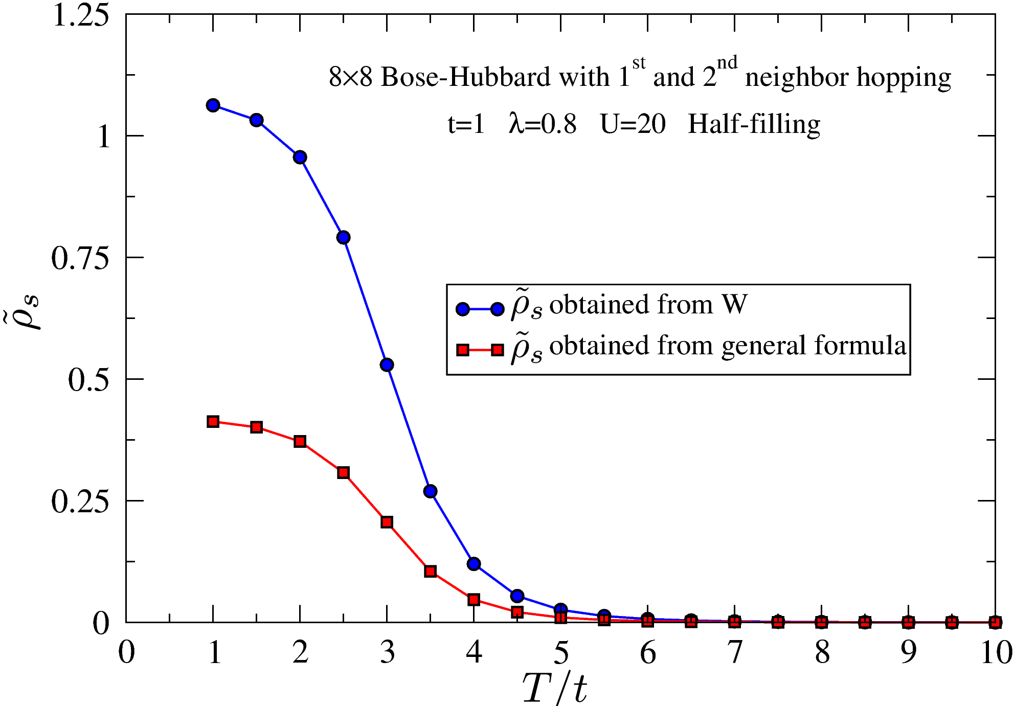
In this section, we illustrate the usefulness of Eq. (69) by considering a Hamiltonian for which the well-known expressions of the superfluid density are not applicable. The model consists of soft-core bosons on a two-dimensional $S\times S$ square lattice described by the Hamiltonian:

$$\hat{\mathcal{H}}_{o} = -t\sum_{\langle p,q\rangle}\big{(}a_{p}^{\dagger}a_{q}^{\phantom{\dagger}}+H.c.\big{)}+\frac{U}{2}\sum_{j}\hat{n}_{j}(\hat{n}_{j}-1)$$ (92)

$$-\lambda\sum_{\langle\langle p,q\rangle\rangle}\big{(}a_{p}^{\dagger}a_{q}^{\phantom{\dagger}}+H.c.\big{)}$$

The sum $\sum_{\langle\langle p,q\rangle\rangle}$ is over all distinct pairs of second-neighboring sites $p$ and $q$. In addition to the discrete operators (54), (55), (57), (59), we define the operator:

$$\vec{\mathcal{Q}}=-i\sqrt{mt/2}\sum_{\langle\langle p,q\rangle\rangle}\big{(}a_{p}^{\dagger}a_{q}^{\phantom{\dagger}}-H.c.\big{)}(\vec{q}-\vec{p})$$ (93)

Calculating the commutator $\big{[}\vec{\mathcal{R}},\hat{\mathcal{H}}_{o}\big{]}$ leads to:

$$\big{[}\vec{\mathcal{R}},\hat{\mathcal{H}}_{o}\big{]}=i\frac{\hbar}{m}\Big{(}\vec{\mathcal{P}}+\frac{\lambda}{t}\vec{\mathcal{Q}}\Big{)}$$ (94)

Therefore, the Hamiltonian (92) does not belong to the class defined by (34), and the expression of the superfluid density given by (80) with $d=2$ is not applicable. Injecting (94) into (69) with $S_{\textrm{\tiny tot}}=S^{2}$, we get the expression:

$$\tilde{\rho}_{s} = \tilde{\rho}-\frac{1}{4tS^{2}}\big{\langle}\hat{\mathcal{T}}\big{\rangle}$$ (95)

$$-\frac{1}{2mS^{2}}\Big{\langle}\vec{\mathcal{P}}\cdot\!\!\int_{0}^{\beta}\!\!e^{\tau\hat{\mathcal{H}}_{o}}\Big{(}\vec{\mathcal{P}}+\frac{\lambda}{t}\vec{\mathcal{Q}}\Big{)}e^{-\tau\hat{\mathcal{H}}_{o}}\textrm{d}\tau\Big{\rangle}$$

Using the SGF algorithmSGF with directed updatesDirectedSGF , it is easy to evaluate (95) for a given configuration of the particle worldlines by defining $n_{\zeta}$ as the number of hoppings in the direction $\zeta$, with $\zeta=\leftarrow,\rightarrow,\uparrow,\downarrow,\swarrow,\nearrow,\searrow,\nwarrow$, the notation being self-explanatory. Then (95) takes the form:

$$\tilde{\rho}_{s} = \frac{1}{4t\beta S^{2}}\big{\langle}\!(n_{{}_{\leftarrow}}\!-\!n_{{}_{\rightarrow}})\!(n_{{}_{\leftarrow}}\!-\!n_{{}_{\rightarrow}}\!+\!n_{{}_{\swarrow}}\!-\!n_{{}_{\nearrow}}\!-\!n_{{}_{\searrow}}\!+\!n_{{}_{\nwarrow}})$$ (96)

$$+(n_{{}_{\downarrow}}-n_{{}_{\uparrow}})(n_{{}_{\downarrow}}-n_{{}_{\uparrow}}+n_{{}_{\swarrow}}-n_{{}_{\nearrow}}+n_{{}_{\searrow}}-n_{{}_{\nwarrow}})\big{\rangle}$$

We have simulated the Hamiltonian (92) with $t=1$, $\lambda=0.8$, and $U=20$, at half-filling ($\tilde{\rho}=\frac{1}{2}$) as a function of temperature. Fig. 9 shows a comparison between the quantity given by the discrete form of Pollock and Ceperley’s formula (80) and our expression (96). This example clearly demonstrates that (80) is not applicable for this Hamiltonian, since it gives a value that is greater than the total density. On the other hand, our expression (96) ensures that $\tilde{\rho}_{s}\in[0;\tilde{\rho}]$.

Figure 9: (Color online) Comparison between the superfluid density (red) obtained from the general expression (96) and the quantity (blue) given by (80) for the Hamiltonian (92). The errorbars are smaller than the symbols’ size.

VIII Multi-species Hamiltonians

The theory developed in sections IV and V can be extended to multi-species Hamiltonians in order to obtain the superfluid density of each component of mixtures. Again, for the sake of simplicity, we consider in the following only the isotropic case. Consider a $d$-dimensional Hamiltonian $\hat{\mathcal{H}}_{o}$ with several species of particles. We denote by $m_{\zeta}$ the mass of a particle of a given species $\zeta$.

VIII.1 Continuous space

By adding the index $\zeta$ to the field operators that appear in (10), (11), and (12), we can define the continuous-space number $\hat{\mathcal{N}}_{\zeta}$, position $\vec{\mathcal{R}}_{\zeta}$, and momentum $\vec{\mathcal{P}}_{\zeta}$ operators associated to each species $\zeta$. As shown by Andreev and BashkinAndreev , the superfluid current $\vec{j}_{s}^{\zeta}$ of a given species $\zeta$ can be carried by the other species. As a result, the superfluid density is a second order tensor, and the superfluid current is given by

$$\vec{j}_{s}^{\zeta}=\rho_{s}^{\zeta\xi}\vec{v}_{s}^{\>\xi},$$ (97)

where $\vec{v}_{s}^{\>\xi}$ is the superfluid velocity of species $\xi$. The friction between the normal components of each species imposes the normal velocity to be the same for all species. However the different species can have different superfluid velocities. For each species $\zeta$, we denote by $\mathcal{F}^{\zeta}$ the frame in which its supefluid component comes to rest, and we denote by $\mathcal{F}^{\prime}$ the frame of the moving walls in which the normal components of all species are at rest. Defining $\vec{v}^{\>\zeta}$ as the velocity of $\mathcal{F}^{\prime}$ with respect to $\mathcal{F}^{\zeta}$, we can define the unitary operator

$$\hat{\mathcal{U}}=e^{-\frac{i}{\hbar}\sum_{\zeta}m_{\zeta}\vec{v}^{\>\zeta}\cdot\vec{\mathcal{R}}_{\zeta}},$$ (98)

and interpret it as the operator that performs for each species $\zeta$ a Galilean transformation from $\mathcal{F}^{\zeta}$ to $\mathcal{F}^{\prime}$. Applying the correspondence principle in the frame $\mathcal{F}^{\prime}$ of the moving walls, the quantum average of the momentum operator of species $\zeta$ must be equal to the classical momentum, which is due to the superfluid only. In this frame, the superfluid velocity of species $\xi$ is $\vec{v}_{s}^{\>\xi}=-\vec{v}^{\>\xi}$. Thus we have:

$$-\rho_{s}^{\zeta\xi}\vec{v}^{\>\xi}\Omega = \frac{1}{\mathcal{Z}_{o}}\textrm{Tr }\vec{\mathcal{P}}_{\zeta}e^{-\beta\hat{\mathcal{H}}_{o}}$$ (99)

$$= \frac{1}{\mathcal{Z}_{o}}\textrm{Tr }\hat{\mathcal{U}}^{\dagger}\vec{\mathcal{P}}_{\zeta}\hat{\mathcal{U}}e^{-\beta\hat{\mathcal{U}}^{\dagger}\hat{\mathcal{H}}_{o}\hat{\mathcal{U}}}$$

$$= \frac{1}{\mathcal{Z}_{o}}\textrm{Tr }\big{(}\vec{\mathcal{P}}_{\zeta}-m_{\zeta}\vec{v}^{\>\zeta}\hat{\mathcal{N}}_{\zeta}\big{)}e^{-\beta\hat{\mathcal{U}}^{\dagger}\hat{\mathcal{H}}_{o}\hat{\mathcal{U}}}$$

Calculating the divergence with respect to $\vec{v}^{\>\xi}$ and taking the limit where all velocities go to zero, we get the expression of the superfluid tensor

$$\rho_{s}^{\zeta\xi}=\rho^{\zeta}\delta_{\zeta\xi}+i\frac{m_{\xi}}{\hbar\Omega d}\Big{\langle}\vec{\mathcal{P}}_{\zeta}\cdot\!\!\int_{0}^{\beta}\!\!\!\!e^{\tau\hat{\mathcal{H}}_{o}}\big{[}\vec{\mathcal{R}}_{\xi},\hat{\mathcal{H}}_{o}\big{]}e^{-\tau\hat{\mathcal{H}}_{o}}\textrm{d}\tau\Big{\rangle},$$ (100)

where $\rho^{\zeta}=m_{\zeta}\langle\hat{\mathcal{N}}_{\zeta}\rangle/\Omega$ is the total density of species $\zeta$.

VIII.2 Discrete space

As before, it is useful to write the kinetic energy of species $\zeta$ as a sum of contributions from the different directions, $\hat{\mathcal{T}}_{\zeta}=\sum_{j}\hat{\mathcal{T}}_{j\zeta}$, and see how the momentum $\vec{\mathcal{P}}_{\zeta}$ transforms under $\hat{\mathcal{U}}$:

$$\hat{\mathcal{U}}^{\dagger}\vec{\mathcal{P}}_{\zeta}\hat{\mathcal{U}}=\vec{\mathcal{P}}_{\zeta}-m_{\zeta}\vec{v}^{\>\zeta}\hat{\mathcal{N}}_{\zeta}+\frac{m_{\zeta}}{2t_{\zeta}}\sum_{j}v_{j}^{\zeta}\hat{j}\hat{\mathcal{T}}_{j\zeta}+\vec{\mathcal{O}}(\vec{v}^{2})$$ (101)

Thus, new terms proportional to $\hat{\mathcal{T}}_{j\zeta}$ need to be subtracted from (99), leading to:

$$\rho_{s}^{\zeta\xi} = \Big{(}\rho^{\zeta}-\frac{m_{\zeta}}{2t_{\zeta}\Omega d}\big{\langle}\hat{\mathcal{T}}_{\zeta}\big{\rangle}\Big{)}\delta_{\zeta\xi}$$ (102)

$$+i\frac{m_{\xi}}{\hbar\Omega d}\Big{\langle}\vec{\mathcal{P}}_{\zeta}\cdot\!\!\int_{0}^{\beta}\!\!\!\!e^{\tau\hat{\mathcal{H}}_{o}}\big{[}\vec{\mathcal{R}}_{\xi},\hat{\mathcal{H}}_{o}\big{]}e^{-\tau\hat{\mathcal{H}}_{o}}\textrm{d}\tau\Big{\rangle}$$

Our previous definition of the dimensionless superfluid density (68) can be generalized to the superfluid density tensor as

$$\tilde{\rho}_{s}^{\zeta\xi}=\frac{\rho_{s}^{\zeta\xi}\Omega}{m_{\xi}S_{\textrm{\tiny tot}}},$$ (103)

Defining the for each species $\zeta$ the associated dimensionless density $\tilde{\rho}^{\zeta}=\rho^{\zeta}\Omega/m_{\zeta}S_{\textrm{\tiny tot}}$, we get:

$$\tilde{\rho}_{s}^{\zeta\xi} = \Big{(}\tilde{\rho}^{\zeta}-\frac{1}{2t_{\zeta}dS_{\textrm{\tiny tot}}}\big{\langle}\hat{\mathcal{T}}_{\zeta}\big{\rangle}\Big{)}\delta_{\zeta\xi}$$ (104)

$$+i\frac{1}{\hbar dS_{\textrm{\tiny tot}}}\Big{\langle}\vec{\mathcal{P}}_{\zeta}\cdot\!\!\int_{0}^{\beta}\!\!\!\!e^{\tau\hat{\mathcal{H}}_{o}}\big{[}\vec{\mathcal{R}}_{\xi},\hat{\mathcal{H}}_{o}\big{]}e^{-\tau\hat{\mathcal{H}}_{o}}\textrm{d}\tau\Big{\rangle}\quad$$

VIII.3 Application to a two-species Hamiltonian with inter-species conversion terms

We consider here a one-dimensional lattice Hamiltonian with $S$ sites that describes atoms and molecules with inter-species conversion termsFeshbach1 ; Feshbach2 , which takes the form

$$\hat{\mathcal{H}}_{o} = -t_{a}\sum_{\langle p,q\rangle}\big{(}a_{p}^{\dagger}a_{q}^{\phantom{\dagger}}+H.c.\big{)}-t_{m}\sum_{\langle p,q\rangle}\big{(}m_{p}^{\dagger}m_{q}^{\phantom{\dagger}}+H.c.\big{)}$$ (105)

$$+\frac{U_{aa}}{2}\sum_{p}\hat{n}_{p}^{a}(\hat{n}_{p}^{a}-1)+\frac{U_{mm}}{2}\sum_{p}\hat{n}_{p}^{m}(\hat{n}_{p}^{m}-1)$$

$$+U_{am}\sum_{p}\hat{n}_{p}^{a}\hat{n}_{p}^{m}+D\sum_{p}\hat{n}_{p}^{m}$$

$$+\sigma\sum_{p}\big{(}a_{p}^{\dagger}a_{p}^{\dagger}m_{p}^{\phantom{\dagger}}+H.c.\big{)},$$

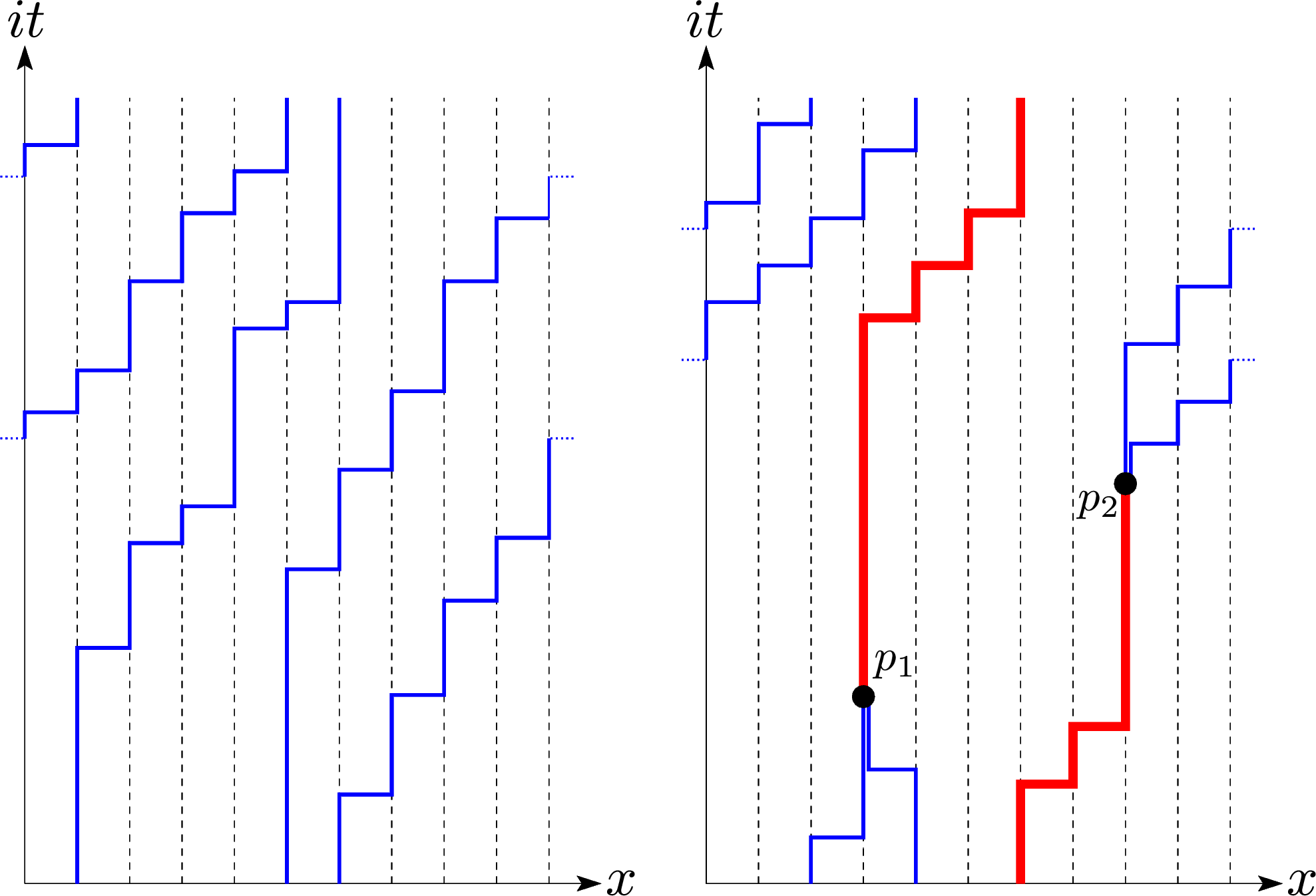
where $a_{p}^{\dagger}$ and $a_{p}^{\phantom{\dagger}}$ (resp. $m_{p}^{\dagger}$ and $m_{p}^{\phantom{\dagger}}$) are the creation and annihilation operators of an atom (resp. a molecule) on site $p$. The operator $\hat{n}_{p}^{a}=a_{p}^{\dagger}a_{p}^{\phantom{\dagger}}$ (resp $\hat{n}_{p}^{m}=m_{p}^{\dagger}m_{p}^{\phantom{\dagger}}$) counts the number of atoms (resp. molecules) on site $p$. The last term in (105) converts a molecule into two atoms and vice-versa. As a result, this Hamiltonian does not conserve the number of atoms nor the number of molecules, but we can define the total density as $\tilde{\rho}^{\textrm{\tiny tot}}=\tilde{\rho}^{a}+2\tilde{\rho}^{m}$ which is conserved. In a path-integral representation, the non-conservation of the number of atoms and molecules means that the atomic and molecular worldlines can be broken (Fig. 10). As pointed in ref.Eckholt , this results in the impossibility to define winding numbers for atoms and for molecules that are topologically conserved. Nevertheless, our general expression of the superfluid density tensor (104) does not rely on any definition of the winding number, and can be easily calculated.

Figure 10: (Color online) Worldline representation of a configuration of the partition function in the space and imaginary time $(x,it)$ plane. The left figure shows a configuration with 3 atoms (blue) when no molecules are formed. In this case, the winding number $W_{a}$ of the atoms can be defined, and the present realization corresponds to $W_{a}=2$. The right figure corresponds to a case when molecules (red) are formed. In this case, the numbers of atoms and molecules depend on imaginary time. Since the paths of the atoms and molecules are undefined between the points $p_{1}$ and $p_{2}$, it is not possible to assign winding numbers to them.

Calculating the commutators of the position operators $\mathcal{R}_{a}$ and $\mathcal{R}_{m}$ with the Hamiltonian (105), we obtain

$$\big{[}\mathcal{R}_{a},\hat{\mathcal{H}}_{o}\big{]}=i\frac{\hbar}{m_{a}}\mathcal{P}_{a}+2\mathcal{C},$$ (106)

$$\big{[}\mathcal{R}_{m},\hat{\mathcal{H}}_{o}\big{]}=i\frac{\hbar}{m_{m}}\mathcal{P}_{m}-\mathcal{C},$$ (107)

where $\mathcal{C}$ is given by:

$$\mathcal{C}=\sigma l\sum_{p}p\big{(}a_{p}^{\dagger}a_{p}^{\dagger}m_{p}^{\phantom{\dagger}}-H.c.\big{)}$$ (108)

Injecting (106) and (107) in (103), we obtain the elements of the superfluid density tensor:

$$\tilde{\rho}_{s}^{aa} = \tilde{\rho}^{a}-\frac{1}{2t_{a}S}\big{\langle}\hat{\mathcal{T}}_{a}\big{\rangle}$$ (109)

$$-\frac{1}{m_{a}S}\big{\langle}\mathcal{P}_{a}\int_{0}^{\beta}\mathcal{P}_{a}(\tau)\textrm{d}\tau\Big{\rangle}$$

$$+\frac{2i}{\hbar S}\big{\langle}\mathcal{P}_{a}\int_{0}^{\beta}\mathcal{C}(\tau)\textrm{d}\tau\big{\rangle}$$

$$\tilde{\rho}_{s}^{mm} = \tilde{\rho}^{m}-\frac{1}{2t_{m}S}\big{\langle}\hat{\mathcal{T}}_{m}\big{\rangle}$$ (110)

$$-\frac{1}{m_{m}S}\big{\langle}\mathcal{P}_{m}\int_{0}^{\beta}\mathcal{P}_{m}(\tau)\textrm{d}\tau\Big{\rangle}$$

$$-\frac{i}{\hbar S}\big{\langle}\mathcal{P}_{m}\int_{0}^{\beta}\mathcal{C}(\tau)\textrm{d}\tau\big{\rangle}$$

$$\tilde{\rho}_{s}^{am} = -\frac{1}{m_{m}S}\big{\langle}\mathcal{P}_{a}\int_{0}^{\beta}\mathcal{P}_{m}(\tau)\textrm{d}\tau\Big{\rangle}$$ (111)

$$-\frac{i}{\hbar S}\big{\langle}\mathcal{P}_{a}\int_{0}^{\beta}\mathcal{C}(\tau)\textrm{d}\tau\big{\rangle}$$

$$\tilde{\rho}_{s}^{ma} = -\frac{1}{m_{a}S}\big{\langle}\mathcal{P}_{m}\int_{0}^{\beta}\mathcal{P}_{a}(\tau)\textrm{d}\tau\Big{\rangle}$$ (112)

$$+\frac{2i}{\hbar S}\big{\langle}\mathcal{P}_{m}\int_{0}^{\beta}\mathcal{C}(\tau)\textrm{d}\tau\big{\rangle}$$

Evaluating (109), (110), (111), and (112) with the SGF method is made easy by defining $n_{L}^{a}$ and $n_{R}^{a}$ (resp. $n_{L}^{m}$ and $n_{R}^{m}$) as the numbers of hoppings of atoms (resp. molecules) to the left and to the right in a given configuration of worldlines, and $n_{m\to a}^{p}$ and $n_{a\to m}^{p}$ as the numbers of conversions of molecules to atoms and atoms to molecules that occur on site $p$. With these definitions, the elements of the superfluid density tensor take the final forms:

$$\tilde{\rho}_{s}^{aa} = \frac{1}{2t_{a}\beta S}\big{\langle}(n_{L}^{a}-n_{R}^{a})^{2}\big{\rangle}$$ (113)

$$+\frac{1}{t_{a}\beta S}\big{\langle}(n_{L}^{a}-n_{R}^{a})\sum_{p}p(n_{m\to a}^{p}-n_{a\to m}^{p})\big{\rangle}\quad$$

$$\tilde{\rho}_{s}^{mm} = \frac{1}{2t_{m}\beta S}\big{\langle}(n_{L}^{m}-n_{R}^{m})^{2}\big{\rangle}$$ (114)

$$-\frac{1}{2t_{m}\beta S}\big{\langle}(n_{L}^{m}-n_{R}^{m})\sum_{p}p(n_{m\to a}^{p}-n_{a\to m}^{p})\big{\rangle}\quad$$

$$\tilde{\rho}_{s}^{am} = \frac{1}{2t_{a}\beta S}\big{\langle}(n_{L}^{a}-n_{R}^{a})(n_{L}^{m}-n_{R}^{m})\big{\rangle}$$ (115)

$$-\frac{1}{2t_{a}\beta S}\big{\langle}(n_{L}^{m}-n_{R}^{m})\sum_{p}p(n_{m\to a}^{p}-n_{a\to m}^{p})\big{\rangle}\quad$$

$$\tilde{\rho}_{s}^{ma} = \frac{1}{2t_{m}\beta S}\big{\langle}(n_{L}^{a}-n_{R}^{a})(n_{L}^{m}-n_{R}^{m})\big{\rangle}$$ (116)

$$+\frac{1}{t_{m}\beta S}\big{\langle}(n_{L}^{a}-n_{R}^{a})\sum_{p}p(n_{m\to a}^{p}-n_{a\to m}^{p})\big{\rangle}\quad$$

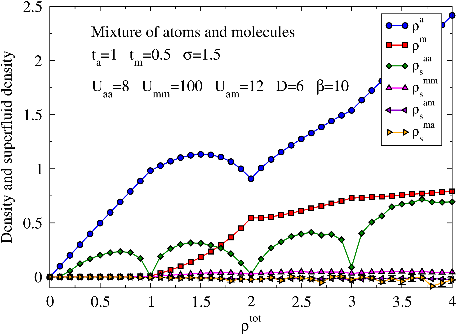
Figure 11 shows the densities $\tilde{\rho}^{a}$ and $\tilde{\rho}^{m}$ of atoms and molecules, and the elements of the superfluid density tensor obtained from (113), (114), (115), and (116) as functions of the total density $\tilde{\rho}^{\textrm{\tiny tot}}$. With the parameters $S=20$, $t_{a}=1$, $t_{m}=0.5$, $\sigma=0.5$, $U_{aa}=8$, $U_{mm}=100$, $U_{am}=12$, $D=6$, and $\beta=10$, our simulations indicate that the phase is incompressible for densities $\tilde{\rho}^{\textrm{\tiny tot}}=1$ and $\tilde{\rho}^{\textrm{\tiny tot}}=2$, and nearly incompressible for $\tilde{\rho}^{\textrm{\tiny tot}}=3$. This is consistent with the features observed in $\tilde{\rho}_{s}^{aa}$, $\tilde{\rho}_{s}^{mm}$, $\tilde{\rho}_{s}^{am}$, and $\tilde{\rho}_{s}^{ma}$, and in agreement with ref.Eckholt .

Figure 11: (Color online) The densities $\tilde{\rho}^{a}$ and $\tilde{\rho}^{m}$ and the elements of the superfluid density tensor $\tilde{\rho}_{s}^{aa}$, $\tilde{\rho}_{s}^{mm}$,$\tilde{\rho}_{s}^{am}$, and $\tilde{\rho}_{s}^{ma}$, as functions of the total density $\tilde{\rho}^{\textrm{\tiny tot}}$. The errorbars are smaller than the symbols’ size.

IX Conclusion

Based on real and thought experiments, we give definitions of the superfluid density for general Hamiltonians, including multi-species Hamiltonians. We derive general expressions that allow us to calculate the superfluid density with path-integral methods. While it is well known that the superfluid density can be related to the response of the free energy to a boundary phase twist or to the fluctuations of the winding number, we show that this is true only for a particular class of Hamiltonians. Our expressions, however, can be applied to any Hamiltonian. In particular, they can be applied to Hamiltonians that do not conserve the number of particles, where the winding number is undefined. By performing a discretization of space with a general change of basis, we obtain formulae for the superfluid density for various lattice geometries. We point to some common mistakes that occur when the energy scale is not correctly reflected in the expression of the superfluid density, and when some correlations are missed because of a non-diagonal metric tensor. Finally, we give two examples of lattice Hamiltonians for which the well-known expressions of the superfluid density are not applicable. We calculate the superfluid densities for these Hamiltonians by evaluating our general expressions by means of quantum Monte Carlo simululations, using the SGF algorithm.