Synchro-thermalization of composite quantum system

Abstract

We study the thermalization of a composite quantum system consisting of several subsystems, where only a small one of the subsystem contacts with a heat bath in equilibrium, while the rest of the composite system is contact free. We show that the whole composite system still can be thermalized after a relaxation time long enough, if the energy level structure of the composite system is connected, which means any two energy levels of the composite system can be connected by direct or indirect quantum transitions. With an example where an multi-level system interacts with a set of harmonic oscillators via non-demolition coupling, we find that the speed of relaxation to the global thermal state is suppressed by the multi-Franck-Condon factor due to the displacements of the Fock states when the degrees of freedom is large.

I Introduction

Isolated quantum systems evolve unitarily according to the Schrödinger equation. When the quantum system is immersed in a canonical heat bath with a temperature $T$, after a relaxation time long enough, it would forget all the initial state information and achieve a canonical state due to the weak interaction with the environment. This process is called canonical thermalization Landau and Lifshitz (1980).

Now we consider the thermalization process for a composite system, which contains several subsystems, where only a small subsystem is contacted with environment [Fig. 1(a)]. We show that if the energy level structure of the composite system is connected, i.e., there exists direct or indirect quantum transitions between any two levels of the system, the whole system would also be thermalized to its canonical thermal state with the bath temperature $T$. The contact of a small part would lead to the global thermalization of the whole system, which is the same as the case that all the subsystems contact with the same heat bath. We call this process synchro-thermalization. Especially, we consider the case that the interactions between each subsystems are non-demolition type, where the interaction coupling does not change the energy of one of the subsystems Dong et al. (2007, 2010). We will explicitly give the condition when the whole composite system can be synchro-thermalized.

On the first sight, this result seems rather counter-intuitive, especially when we consider the case that the rest part of the composite system, which does not contact with the environment, may be quite large and even tend to be infinite. To solve this puzzle, we consider an example where an $N$-level system interacts with a set of $M$ harmonic oscillators via non-demolition coupling. We show that the relaxation rate is suppressed by a multi-Franck-Condon factor Franck and Dymond (1926); Condon (1926); Lax (1952): when the degrees of freedom become large, the speed of global relaxation to the thermal state would tend to be zero. That means, the larger the composite system is, the harder it is to thermalize it. And we call this effect the Franck-Condon blockade Koch and von Oppen (2005) of thermalization.

We arrange our paper as follows. In Sec. II, we give a review on the general situation of thermalization. In Sec. III, we show the connectivity and thermalization of composite systems. In Sec. IV, we discuss a specific model where the composite system consists an $N$-level system and an harmonic oscillator. In Sec. V, we show how the thermalization rate is blockaded by the Franck-Condon factor when the scale of the subsystem free of contact become large. Finally we draw summary in Sec. VI.

II Thermalization of a general system

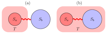
Figure 1: (Colored online) Demonstration of a composite system consisting two interacting parts. (a) Only $S_{a}$ contacts with a heat bath with temperature $T$, while $S_{b}$ does not. (b) Both parts contact with the heat bath directly.

In order to conveniently use the notations in discussions about the synchro-thermalization for a composite system, we review some previous result about the thermalization of a general system first. We write down the Hamiltonian for the system in the eigen basis $\{|n\rangle\}$ as follows,

$$\hat{H}_{S}=\sum_{n}\varepsilon_{n}|n\rangle\langle n|,$$ (1)

where $\varepsilon_{n}$ is the corresponding eigen energy.

The system is contacted with a heat bath via the interaction

$$\hat{H}_{SB}=\sum_{\alpha}\hat{A}_{\alpha}\otimes\hat{R}_{\alpha},$$ (2)

where $\hat{A}_{\alpha}$ and $\hat{R}_{\alpha}$ are operators of the system and the heat bath. In the interaction picture of $\hat{H}_{S}+\hat{H}_{B}$, the system operator $\hat{A}_{\alpha}(t)=\sum_{\omega}\tilde{A}_{\alpha}(\omega)e^{-i\omega t}$ is decomposed according to the oscillation frequencies, and

$$\tilde{A}_{\alpha}(\omega)=\sum_{\varepsilon_{n}-\varepsilon_{m}=\omega}\langle m|\hat{A}_{\alpha}|n\rangle|m\rangle\langle n|$$ (3)

corresponds to the spectral decomposition of system operator $\hat{A}_{\alpha}(t)$ with respect to the eigen basis $\{|n\rangle\}$.

With the Born-Markovian approximation, the master equation for this composite system Breuer and Petruccione (2002),

$$\dot{\rho}= \sum_{\omega,\alpha\beta}\gamma_{\alpha\beta}(\omega)\Big{(}\tilde{A}_{\beta}(\omega)\rho\tilde{A}_{\alpha}^{\dagger}(\omega)-\frac{1}{2}\{\tilde{A}_{\alpha}^{\dagger}(\omega)\tilde{A}_{\beta}(\omega),\,\rho\}_{+}\Big{)},$$

is used to describe the open system dynamics. Here we omitted the Lamb shift term which has no effect on the thermalization. The generalized relaxation rates,

$$\gamma_{\alpha\beta}(\omega)=\int_{-\infty}^{+\infty}d\tau\,e^{i\omega\tau}\langle\hat{R}_{\alpha}^{\dagger}(\tau)\hat{R}_{\beta}(0)\rangle,$$ (4)

are defined by the bath correlation functions $\langle\hat{R}_{\alpha}^{\dagger}(\tau)\hat{R}_{\beta}(0)\rangle$.

According to the Born approximation, the heat bath keeps unchanged, i.e., $\rho_{B}(t)\simeq{\cal Z}_{B}^{-1}\exp[-\beta_{T}\hat{H}_{B}]$. Thus the above finite temperature bath correlation functions $\langle\hat{R}_{\alpha}^{\dagger}(\tau)\hat{R}_{\beta}(0)\rangle$ satisfy the Kubo-Martin-Schwinger condition Kubo (1957); Martin and Schwinger (1959)

$$\langle\hat{R}_{\alpha}^{\dagger}(\tau)\hat{R}_{\beta}(0)\rangle=\langle\hat{R}_{\alpha}(0)\hat{R}_{\beta}^{\dagger}(\tau+i\beta_{T})\rangle.$$ (5)

It is noticed that the generalized relaxation rates $\gamma_{\alpha\beta}(\omega)$ satisfy the following relation,

$$\gamma_{\alpha\beta}(-\omega)=e^{-\beta_{T}\omega}\gamma_{\beta\alpha}(\omega),$$ (6)

which is the key point to lead to detailed balance equilibrium Le Bellac et al. (2004).

The dynamics of the population of the system, denoted as $P_{n}(t):=\rho_{n,n}(t)$, is decoupled from that of the off-diagonal terms $\rho_{n,m}(t)$, and can be described by the following Pauli master equation,

$$\dot{P}_{n}=\sum_{m}W(n\leftarrow m)P_{m}-W(m\leftarrow n)P_{n},$$ (7)

where

$$W(n\leftarrow m)=\sum_{\alpha,\beta}\gamma_{\alpha\beta}(\varepsilon_{m}-\varepsilon_{n})\langle m|\hat{A}_{\alpha}|n\rangle\langle n|\hat{A}_{\beta}|m\rangle,$$ (8)

and $W(n\leftarrow m)$ is the time-independent probability transition rate from $|m\rangle$ to $|n\rangle$. It follows from Eq. (6) that the transition rates satisfies,

$$W(m\leftarrow n)e^{-\beta_{T}\varepsilon_{n}}-W(n\leftarrow m)e^{-\beta_{T}\varepsilon_{m}}=0.$$ (9)

The above derivations have been given in many literatures Breuer and Petruccione (2002). Here we focus our attention on the transition structure of the energy levels induced by the coupling to the heat bath. We would show that whether the whole system can be thermalized to its unique thermal state is determined by the connectivity of the transition structure of the energy levels.

If $W(n\leftarrow m)\neq 0$, there exists direct probability transition between the two levels $|n\rangle\leftrightarrow|m\rangle$ . When $W(m\leftarrow n)=0$, though there is no direct transition between $|n\rangle$ and $|m\rangle$, the indirect transitions still may happen which is mediated by some other levels $|k_{i}\rangle$, that is, the probability transition between $|n\rangle$ and $|m\rangle$ can be completed by a mediating path $|n\rangle\leftrightarrow|k_{1}\rangle\leftrightarrow|k_{2}\rangle\leftrightarrow\dots\leftrightarrow|k_{t}\rangle\leftrightarrow|m\rangle$.

Here we use the concept of connectivity in topology to describe such transition structure of the energy levels. We say the two levels $|n\rangle$ and $|m\rangle$ are path-connected, or connected by a path, if and only if there exists a path, which is represented by an ordered series $\{k_{1},\,k_{2},\,\dots,\,k_{t}\}$, such that $W(n\leftarrow k_{1})\neq 0$, $W(m\leftarrow k_{t})\neq 0$ and $W(k_{i}\leftarrow k_{i+1})\neq 0$ for any $i$. We say the energy structure of the whole system is connected, if and only if any two energy levels are path-connected [Fig. 2(a)], otherwise, we say the energy structure is disconnected [Fig. 2(b)].

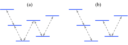
Figure 2: (Colored online) Transition structure of the energy levels, (a) connected (b) disconnected.

Next, we study the thermalization of the system with the consideration of topology mentioned above. According to Eq. (9), the equilibrium steady state requires that Spohn (1977); Le Bellac et al. (2004); Zhang et al. (2012)

$$W(n\leftarrow m)P_{m}-W(m\leftarrow n)P_{n}$$

$$= W(n\leftarrow m)\Big{[}P_{m}-e^{-\beta_{T}(\varepsilon_{m}-\varepsilon_{n})}P_{n}\Big{]}=0.$$ (10)

If $W(n\leftarrow m)\neq 0$, i.e., there exists direct transition between $|n\rangle$ and $|m\rangle$, so that

$$P_{n}:P_{m}=e^{-\beta_{T}\varepsilon_{n}}:e^{-\beta_{T}\varepsilon_{m}}.$$ (11)

If $W(n\leftarrow m)=0$, but $|n\rangle$ and $|m\rangle$ are connected by a path, denoted as $\{k_{1},\,k_{2},\,\dots,\,k_{t}\}$, we have $W(n\leftarrow k_{1})\neq 0$, $W(m\leftarrow k_{t})\neq 0$ and $W(k_{i}\leftarrow k_{i+1})\neq 0$. Thus, with the same reason as above, we have

$$P_{n} :P_{k_{1}}:\dots:P_{k_{t}}:P_{m}$$

$$= e^{-\beta_{T}\varepsilon_{n}}:e^{-\beta_{T}\varepsilon_{k_{1}}}:\dots:e^{-\beta_{T}\varepsilon_{k_{t}}}:e^{-\beta_{T}\varepsilon_{m}}.$$ (12)

Therefore, when the energy structure of the system is connected, the above proportion series includes all the energy levels and that gives the canonical state

$$\rho=\frac{\sum_{n}e^{-\beta_{T}\varepsilon_{n}}|n\rangle\langle n|}{\sum_{n}e^{-\beta_{T}\varepsilon_{n}}}={\cal Z}^{-1}e^{-\beta_{T}\hat{H}_{S}}.$$ (13)

When the energy level structure is not connected, but the whole Hilbert space can be decomposed into two connected subspaces ${\cal V}_{1}$ and ${\cal V}_{2}$ [Fig. 2(b)], e.g., spanned by $\{|n_{1}\rangle\}$ and $\{|n_{2}\rangle\}$ respectively, we have two independent series,

$$P_{n_{1}}:P_{m_{1}}:\dots =e^{-\beta_{T}\varepsilon_{n_{1}}}:e^{-\beta_{T}\varepsilon_{m_{1}}}:\dots,$$ (14a)

$$P_{n_{2}}:P_{m_{2}}:\dots =e^{-\beta_{T}\varepsilon_{n_{2}}}:e^{-\beta_{T}\varepsilon_{m_{2}}}:\dots,$$ (14b)

but we cannot determine further relation between the two series, which should be determined from the initial state. Denoting $p_{i}$ as the probability projected into the subspace ${\cal V}_{i}$ from the initial state, it can be verified that

$$\rho=p_{1}\rho_{1}^{\mathrm{th}}+p_{2}\rho_{2}^{\mathrm{th}}$$ (15)

is the steady state, where

$$\rho_{i}^{\mathrm{th}}:={\cal Z}_{i}^{-1}\sum_{n_{i}}e^{-\beta_{T}\varepsilon_{n_{i}}}|n_{i}\rangle\langle n_{i}|$$ (16)

can be regarded as the partial “thermal state” for the connected subspace ${\cal V}_{i}$.

It follows from Eq. (15) that part of the initial state information of the system can be preserved if the energy level structure is not connected. This is different from the connected case where all the initial state information is erased and the system is fully thermalized in the steady state.

Now we summarize the above results about the thermalization process as the following proposition.

Proposition: If the energy level structure of the system is connected, the system can be thermalized to its canonical thermal state, when it contacts with a equilibrium heat bath.

III Connectivity of composite system and canonical thermalization

III.1 Connected case

Now we study the synchro-thermalization for a composite system, which consists two subsystems $S_{a}$ and $S_{b}$ coupled with each other. According to the proposition in the last section, we need to study whether the energy level structure of the composite system is connected. Generally, the Hamiltonian for the whole system is

$$\hat{H}_{S}=\hat{H}_{a}+\hat{H}_{b}+\hat{V}_{ab},$$ (17)

where $\hat{H}_{a}=\sum_{\mathsf{p}}\varepsilon_{\mathsf{p}}^{a}|\mathsf{p}\rangle_{a}\langle\mathsf{p}|$ and $\hat{H}_{b}=\sum_{n}\epsilon_{n}^{b}|n\rangle_{b}\langle n|$. We denote the eigen state of $\hat{H}_{a}$, $\hat{H}_{b}$ by $\{|\mathsf{p}\rangle_{a}\}$, $\{|n\rangle_{b}\}$, and $\varepsilon_{\mathsf{p}}^{a}$, $\epsilon_{n}^{b}$ are the corresponding eigen energies. The Hamiltonian of the composite system $\hat{H}_{S}$ is diagonalized as $\hat{H}_{S}=\sum_{\mathbf{n}}E_{\mathbf{n}}|\mathbf{n}\rangle\langle\mathbf{n}|$, where $|\mathbf{n}\rangle$ is usually some superposition of the product states $|\mathsf{p}\rangle_{a}\otimes|n\rangle_{b}$,

$$|\mathbf{n}\rangle=\sum_{\mathsf{p},n}\Psi_{\mathsf{p},n}^{\mathbf{n}}|\mathsf{p}\rangle_{a}|n\rangle_{b}.$$ (18)

And $E_{\mathbf{n}}$ is the eigen energy of the composite system.

The subsystem $S_{a}$ contacts with a heat bath via the following interaction, $\hat{H}_{SB}=\sum_{\alpha}\hat{A}_{\alpha}\otimes\hat{R}_{\alpha}$, where $\hat{A}_{\alpha}$ and $\hat{R}_{\alpha}$ are operators of $S_{a}$ and the heat bath respectively. We suppose that $S_{b}$ does not contact with any heat bath directly.

$\hat{A}_{\alpha}$ is expanded in the eigen basis of $\hat{H}_{S}$ as $\hat{A}_{\alpha}=\sum_{\mathbf{n},\mathbf{m}}\langle\mathbf{n}|\hat{A}_{\alpha}|\mathbf{m}\rangle\,|\mathbf{n}\rangle\langle\mathbf{m}|$. Then the transition rate of the composite system becomes

$$W(\mathbf{n}\leftarrow\mathbf{m})=\sum_{\alpha,\beta}\gamma_{\alpha\beta}(E_{\mathbf{m}}-E_{\mathbf{n}})\langle\mathbf{m}|\hat{A}_{\alpha}|\mathbf{n}\rangle\langle\mathbf{n}|\hat{A}_{\beta}|\mathbf{m}\rangle.$$

For example, we consider the case that $S_{a}$ is coupled with $S_{b}$ via the interaction of the non-demolition type, i.e., $[\hat{V}_{ab},\hat{H}_{a}]=0$, which means that the energy of $S_{a}$ does not change due to such interaction with $S_{b}$ in the absence of the environment. In this case, the eigen state of the composite system has the form of $|\mathsf{p},n\rangle=|\mathsf{p}\rangle_{a}\otimes|\phi_{n}^{(\mathsf{p})}\rangle_{b}$, where $|\phi_{n}^{(\mathsf{p})}\rangle_{b}$ is the eigen state of the effective $\mathsf{p}$-branch Hamiltonian,

$$\hat{H}_{b}^{(\mathsf{p})}:=\hat{H}_{b}+\langle\mathsf{p}|\hat{V}_{ab}|\mathsf{p}\rangle_{a},$$ (19)

of the subsystem $S_{b}$. The original energy level $|\mathsf{p}\rangle_{a}$ is splitted into some sub levels $|\mathsf{p},n\rangle$ due to the interaction. We can write down the transition rates of the composite system

$$W(\mathsf{p}n\leftarrow\mathsf{q}m)= \sum_{\alpha,\beta}\gamma_{\alpha\beta}(E_{\mathsf{q}m}-E_{\mathsf{p}n})$$ (20)

$$\times|\langle\phi_{n}^{(\mathsf{p})}|\phi_{m}^{(\mathsf{q})}\rangle|^{2}\langle\mathsf{p}|\hat{A}_{\alpha}|\mathsf{q}\rangle\langle\mathsf{q}|\hat{A}_{\beta}|\mathsf{p}\rangle.$$

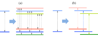
Figure 3: (Colored online) Demonstration for the connectivity of the sideband states of a composite system, (a) connected (b) disconnected.

In most cases, $W(\mathsf{p}n\leftarrow\mathsf{q}m)$ dose not vanish, since the matrix elements $\langle\mathbf{m}|\hat{A}_{\alpha}|\mathbf{n}\rangle$ do not vanish simultaneously when the indices $\mathbf{m},\,\mathbf{n},\,\alpha$ take values in their domains. If the original energy levels $|\mathsf{p}\rangle$ of $S_{a}$ are connected in absence of the interaction with $S_{b}$, the energy levels of the coupled composite system $|\mathsf{p},n\rangle$ are still connected [Fig. 3(a)]. Therefore, according to the proposition in the last section, the whole composite system can be thermalized simultaneously to the canonical state

$$\rho_{\mathrm{th}}={\cal Z}^{-1}\exp[-\beta_{T}(\hat{H}_{a}+\hat{H}_{b}+\hat{H}_{ab})].$$

III.2 Disconnected case

Now we present an example where the energy structure of the composite system is not connected. We consider the interaction Hamiltonian $\hat{V}_{ab}$ of non-demolition type for both $S_{a}$ and $S_{b}$, i.e., $[\hat{V}_{ab},\,\hat{H}_{a/b}]=0$. In this case, $S_{a}$ and $S_{b}$ do not exchange energy with each other, and $\hat{V}_{ab}$ has the form of

$$\hat{V}_{ab}=\sum_{\mathsf{p},n}\,g_{\mathsf{p},n}|\mathsf{p}\rangle_{a}\langle\mathsf{p}|\otimes|n\rangle_{b}\langle n|,$$ (21)

and the eigenstates of $\hat{H}_{ab}$ are $|\mathsf{p},n\rangle=|\mathsf{p}\rangle_{a}\otimes|n\rangle_{b}$, with eigen energy $E_{\mathsf{p}n}=\varepsilon_{\mathsf{p}}^{a}+\epsilon_{n}^{b}+g_{\mathsf{p},n}$. We obtain the transition rates of the composite system as

$$W(\mathsf{p}n\leftarrow\mathsf{q}m) =$$

$$\delta_{mn}\sum_{\alpha,\beta} \gamma_{\alpha\beta}(E_{\mathsf{q}m}-E_{\mathsf{p}n})\langle\mathsf{p}|\hat{A}_{\alpha}|\mathsf{q}\rangle\langle\mathsf{q}|\hat{A}_{\beta}|\mathsf{p}\rangle.$$

Notice that $\gamma_{\alpha\beta}(\omega)$ is usually a smooth function and varies quite slowly with $\omega$, thus we have $W(\mathsf{p}n\leftarrow\mathsf{q}m)\simeq\delta_{mn}W(\mathsf{p}\leftarrow\mathsf{q})$, which means that if the states $|\mathsf{p}\rangle$ and $|\mathsf{q}\rangle$ of $S_{a}$ are connected, the sideband states $|\mathsf{p},n\rangle$ and $|\mathsf{q},n\rangle$ are also connected, but $|\mathsf{p},n\rangle$ and $|\mathsf{q},m\rangle$ with $m\neq n$ are not, as demonstrated in Fig. 3(b). As a result, the energy structure of the composite system is not connected. According to the discussion in the last section, the final steady state of the composite system is $\rho=\sum_{n}p_{n}\rho_{n}^{\mathrm{th}}$, where

$$\rho_{n}^{\mathrm{th}}={\cal Z}_{n}^{-1}\sum_{\mathsf{p}}e^{-\beta_{T}E_{\mathsf{p}n}}|\mathsf{p},n\rangle\langle\mathsf{p},n|,$$ (22)

and the probabilities $p_{n}$ are determined by the initial state. Therefore, the whole composite system cannot be synchro-thermalized to the canonical state in this situation.

For example, we consider a two-level qubit coupled to a resonator via the following Hamiltonian,

$$\hat{H}_{\mathrm{Q}+\mathrm{L}} =\hat{H}_{\mathrm{Q}}+\hat{H}_{\mathrm{R}}+\hat{V}_{\mathrm{QR}}$$ (23)

$$=-\frac{\varepsilon_{\mathrm{Q}}}{2}\hat{\sigma}^{z}+\omega_{\mathrm{L}}\hat{a}^{\dagger}\hat{a}+g\,\hat{\sigma}^{z}\cdot\hat{a}^{\dagger}\hat{a},$$

and we have $[\hat{H}_{\mathrm{Q}},\,\hat{V}_{\mathrm{QR}}]=[\hat{H}_{\mathrm{R}},\,\hat{V}_{\mathrm{QR}}]=0$. This model can be implemented by a Josephson qubit coupled to a superconducting resonator Lupaşcu et al. (2007); Schuster et al. (2007), or by an atom inside an optical cavity Brune et al. (1990), in the dispersive regime with large detuning. The resonator is contact free, while the qubit is contacted with a heat bath via

$$\hat{H}_{SB}=\hat{\sigma}^{+}\cdot\sum\eta_{k}\hat{b}_{k}+\hat{\sigma}^{-}\cdot\sum\eta_{k}^{*}\hat{b}_{k}^{\dagger}.$$

The eigen states of $\hat{H}_{\mathrm{Q+L}}$ are $\{|0,n\rangle,\,|1,n\rangle\}$. We can check that transition happens only between $|0,n\rangle$ and $|1,n\rangle$, but does not happen between $|\mathsf{p},n\rangle$ and $|\mathsf{q},m\rangle$ for $m\neq n$. The energy structure of the composite system is disconnected as Fig. 3(b). For this system, the steady state is

$$\rho^{\mathrm{th}} =\sum_{n}p_{n}\rho_{n}^{\mathrm{th}},$$ (24)

$$\rho_{n}^{\mathrm{th}} =\frac{1}{1+e^{\beta_{T}\varepsilon_{\mathrm{Q}}}}|0,n\rangle\langle 0,n|+\frac{e^{\beta_{T}\varepsilon_{\mathrm{Q}}}}{1+e^{\beta_{T}\varepsilon_{\mathrm{Q}}}}|1,n\rangle\langle 1,n|,$$

and $p_{n}$ is determined by the initial condition.

IV Synchro-thermalization of composite system with non-demolition coupling

In this section, we consider an example of this synchro-thermalization of a composite system consisting of an $N$-level system and an harmonic oscillator interacting with each other via non-demolition coupling. This composite system is described by the following Hamiltonian,

$$\hat{H}_{S} =\hat{H}_{\mathrm{NLS}}+\hat{H}_{\mathrm{HO}}+\hat{V}_{\mathrm{N-H}}$$ (25)

$$=\sum_{\mathsf{p}=0}^{N-1}\epsilon_{\mathsf{p}}|\mathsf{p}\rangle\langle\mathsf{p}|+\Omega\hat{a}^{\dagger}\hat{a}+\sum_{\mathsf{p}}\xi_{\mathsf{p}}|\mathsf{p}\rangle\langle\mathsf{p}|\,\big{(}\hat{a}+\hat{a}^{\dagger}).$$

The $N$-level system is contacted with a heat bath. However, the harmonic oscillator does not couple to the environment directly. In the weak coupling limit, the heat bath could be modeled as a collection of harmonic oscillators linearly coupled to the system Caldeira and Leggett (1983). Thus the $N$-level system exchanges energy with a boson bath via the following coupling,

$$\hat{H}_{SB}=\sum_{k}\sum_{\mathsf{p}>\mathsf{q}}^{N-1}g_{k}\big{(}|\mathsf{p}\rangle\langle\mathsf{q}|\,\hat{b}_{k}+|\mathsf{q}\rangle\langle\mathsf{p}|\,\hat{b}_{k}^{\dagger}),$$ (26)

while the bath Hamiltonian reads $\hat{H}_{B}=\sum_{k}\omega_{k}\hat{b}_{k}^{\dagger}\hat{b}_{k}$. Here we make a simplification that $g_{k}$ only depend on the bath mode $k$ but not on the energy level $\mathsf{p},\,\mathsf{q}$, without loss of generality.

The Hamiltonian of the composite system Eq. (25) is diagonalized with the help of $N$ sets of displaced harmonic oscillator operators corresponding to the coupling with each energy level $|\mathsf{p}\rangle$ Dong et al. (2007, 2010),

$$\hat{H}_{S}=\sum_{\mathsf{p}=0}^{N-1}|\mathsf{p}\rangle\langle\mathsf{p}|\Big{[}\Omega\,\hat{D}^{\dagger}(\alpha_{\mathsf{p}})\hat{a}^{\dagger}\hat{a}\hat{D}^{\dagger}(\alpha_{\mathsf{p}})+\varepsilon_{\mathsf{p}}\Big{]},$$ (27)

where $\alpha_{\mathsf{p}}=\xi_{\mathsf{p}}/\Omega$ and $\varepsilon_{\mathsf{p}}=\epsilon_{\mathsf{p}}-\xi_{\mathsf{p}}^{2}/\Omega$ are the displacement and energy shift respectively. And we define the displacement operator as $\hat{D}(\alpha_{\mathsf{p}})=\exp[\alpha_{\mathsf{p}}(\hat{a}^{\dagger}-\hat{a})]$, which satisfies $\hat{D}^{\dagger}(\alpha_{\mathsf{p}})\hat{a}\hat{D}(\alpha_{\mathsf{p}})=\hat{a}+\alpha_{\mathsf{p}}$. Then we obtain the eigenstate of $\hat{H}_{S}$ as

$$|\mathsf{p},n\rangle=|\mathsf{p}\rangle\otimes[\hat{D}^{\dagger}(\alpha_{\mathsf{p}})|n\rangle_{b}],$$ (28)

and eigen energy is $E_{\mathsf{p},n}=n\Omega+\varepsilon_{\mathsf{p}}.$ Here $|n\rangle_{b}$ is the Fock state of the original harmonic oscillator. We notice that each Fock state $|n\rangle_{b}$ is splitted into $N$ levels $|\mathsf{p},n\rangle$ and forms a side-band structure caused by the coupling with the $N$-level system.

Under the composite eigen basis $\{|\mathsf{p},n\rangle\}$ of $\hat{H}_{S}$, the interaction Hamiltonian with the bath $\hat{H}_{SB}$ is expressed as

$$\hat{H}_{SB}=\sum_{m,n=0}^{\infty}\sum_{\mathsf{p}>\mathsf{q}}^{N-1}\langle n_{\mathsf{p}}|m_{\mathsf{q}}\rangle\,|\mathsf{p},n\rangle\langle\mathsf{q},m|\big{(}\sum_{k}g_{k}\hat{b}_{k}\big{)}+\mathbf{h.c.}$$ (29)

Here, $|n_{\mathsf{p}}\rangle:=\hat{D}^{\dagger}(\alpha_{\mathsf{p}})|n\rangle_{b}$ is the displaced Fock state according to the coupling with $|\mathsf{p}\rangle$.

In comparison with the original system-bath coupling Eq. (26), the effective coupling strengths of the composite system to the heat bath are modified by a Franck-Condon factor $\langle n_{\mathsf{p}}|m_{\mathsf{q}}\rangle$, which is the overlap integral of the wave function of displaced Fock states Franck and Dymond (1926); Condon (1926); Lax (1952) (Fig. 4). As shown as follows, the Franck-Condon factor suppresses the relaxation rates.

For the boson bath with the coupling spectrum

$$J(\omega):=2\pi\sum_{k}\left|g_{k}\right|^{2}\delta(\omega-\omega_{k}),\quad\omega\geq 0,$$ (30)

the Born-Markovian approximation gives a master equation for the dynamics of this composite system Breuer and Petruccione (2002),

$$\dot{\rho}=\sum_{\mathsf{p}n,\mathsf{q}m}^{\mathsf{q}\neq\mathsf{p}}\Gamma(\Delta_{\mathsf{p}n,\mathsf{q}m}) \Big{(}\hat{L}_{\mathsf{p}n,\mathsf{q}m}\rho\hat{L}_{\mathsf{p}n,\mathsf{q}m}^{\dagger}$$

$$-\frac{1}{2}\{\hat{L}_{\mathsf{p}n,\mathsf{q}m}^{\dagger}\hat{L}_{\mathsf{p}n,\mathsf{q}m},\rho\}\Big{)},$$ (31)

where $\hat{L}_{\mathsf{p}n,\mathsf{q}m}:=|\mathsf{p}n\rangle\langle\mathsf{q}m|$ is the Lindblad operator, and $\Delta_{\mathsf{p}n,\mathsf{q}m}:=E_{\mathsf{p}n}-E_{\mathsf{q}m}$. $\Gamma(\Delta_{\mathsf{p}n,\mathsf{q}m})$ is the dissipation rate between the two levels $|\mathsf{p},n\rangle$ and $|\mathsf{q},m\rangle$, and

$$\Gamma_{\mathsf{p}n,\mathsf{q}m}(\omega)=\begin{cases}\left|\langle n_{\mathsf{p}}|m_{\mathsf{q}}\rangle\right|^{2}J(\omega)N(\omega),&\omega\geq 0\\ \left|\langle n_{\mathsf{p}}|m_{\mathsf{q}}\rangle\right|^{2}J(|\omega|)[N(|\omega|)+1],&\omega<0\end{cases}$$

The Franck-Condon factor also appears in this dissipation rate. The norm $|\langle n_{\mathsf{p}}|m_{\mathsf{q}}\rangle|\leq 1$ gives that the relaxation rates are suppressed by the Franck-Condon factor (Fig. 4).

The rate equation about the dynamics of the energy population $P_{\mathsf{p}n}:=\langle\mathsf{p}n|\rho|\mathsf{p}n\rangle$,

$$\dot{P}_{\mathsf{p}n}=\sum_{\mathsf{q},m}^{\mathsf{q}\neq\mathsf{p}}W(\mathsf{p}n\leftarrow\mathsf{q}m)P_{\mathsf{q}m}-W(\mathsf{q}m\leftarrow\mathsf{p}n)P_{\mathsf{p}n},$$ (32)

is obtained from the above master equation, which is decoupled from that of the off-diagonal terms. Here $W(\mathsf{p}n\leftarrow\mathsf{q}m)=\Gamma(\Delta_{\mathsf{p}n,\mathsf{q}m})$ is the population transition rate. The steady state condition requires $\dot{P}_{\mathsf{p}n}=0$, which gives,

$$\left|\langle n_{\mathsf{p}}|m_{\mathsf{q}}\rangle\right|^{2}J(\Delta_{\mathsf{p}n,\mathsf{q}m})\times$$

$$\Big{[}N(\Delta_{\mathsf{p}n,\mathsf{q}m})P_{\mathsf{q}m}- \big{(}N(\Delta_{\mathsf{p}n,\mathsf{q}m})+1\big{)}P_{\mathsf{p}n}\Big{]}=0,$$

for all $E_{\mathsf{p}n}>E_{\mathsf{q}m}$ with $\mathsf{p}\neq\mathsf{q}$.

For any two different levels $|\mathsf{p},n\rangle$ and $|\mathsf{q},m\rangle$, where $\mathsf{p}\neq\mathsf{q}$, we have $W(\mathsf{p}n\leftarrow\mathsf{q}m)\neq 0$. Thus, under the mediation of the environment, the eigenstates of the composite system $|\mathsf{p}n\rangle$ are connected. And the steady population of each two eigenstates satisfies the Boltzmann distribution

$$P_{\mathsf{p}n}:P_{\mathsf{q}m}=e^{-\beta_{T}E_{\mathsf{p}n}}:e^{-\beta_{T}E_{\mathsf{q}m}}.$$

Therefore, the whole composite state can be stabilized to its canonical thermal state $\rho_{\mathrm{th}}={\cal Z}^{-1}\exp[-\beta(\hat{H}_{\mathrm{NLS}}+\hat{H}_{\mathrm{HO}}+\hat{V}_{\mathrm{N-H}})]$ when $t\rightarrow\infty$. The composite system is synchro-thermalized as we discussed in Sec. III-A.

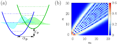
Figure 4: (Colored online) (a) Franck-Condon overlap integral for the displaced Fock states (b) Numerical demonstration for $|\langle n_{\mathsf{p}}|m_{\mathsf{q}}\rangle|=|\langle n|\hat{D}(\alpha_{\mathsf{q}}-\alpha_{\mathsf{p}})|m\rangle|$, where we set $\alpha_{\mathsf{q}}-\alpha_{\mathsf{p}}=1.5$.

V Franck-Condon blockade

We have shown that for a composite system, a partial contact with a heat bath would cause global thermalization. It seems that even if the subsystem contacted with the heat bath is quite small while the rest part tends to be infinitely large, the whole system still can be thermalized globally. In this sense, the above result is rather counter-intuitive.

In order to solve this puzzle, we consider the subsystem $S_{b}$ consists of $M$ harmonic oscillators. $M$ characterizes the scale of the subsystem free of the coupling to the bath. We will see that indeed the global thermalization rate of the whole system decreases rapidly when the scale of the whole composite system becomes large.

We generalize the above example by using $M$ harmonic oscillators to replace the single one coupled to the $N$-level system. Then the system Hamiltonian reads

$$\hat{H}_{S}=\sum_{\mathsf{p}=0}^{N-1}\epsilon_{\mathsf{p}}|\mathsf{p}\rangle\langle\mathsf{p}| +\sum_{i=1}^{M}\Omega_{i}\hat{a}_{i}^{\dagger}\hat{a}_{i}$$

$$+\sum_{i,\mathsf{p}}\xi_{i,\mathsf{p}}|\mathsf{p}\rangle\langle\mathsf{p}|\,\big{(}\hat{a}_{i}+\hat{a}_{i}^{\dagger}),$$ (33)

which is diagonalized as

$$\hat{H}_{S}=\sum_{i,\mathsf{p}}\Big{[}\Omega_{i}\,\hat{D}^{\dagger}(\alpha_{i,\mathsf{p}})\hat{a}_{i}^{\dagger}\hat{a}_{i}\hat{D}^{\dagger}(\alpha_{i,\mathsf{p}})+\varepsilon_{i,\mathsf{p}}\Big{]}\,|\mathsf{p}\rangle\langle\mathsf{p}|,$$ (34)

where $\alpha_{i,\mathsf{p}}$ and $\varepsilon_{i,\mathsf{p}}$ are the displacement and energy shift according to the $i$-th harmonic oscillator and level-$\mathsf{p}$, and $\alpha_{i,\mathsf{p}}:=\xi_{i,\mathsf{p}}/\Omega_{i},\,\varepsilon_{i,\mathsf{p}}:=\epsilon_{i,\mathsf{p}}-\xi_{i,\mathsf{p}}^{2}/\Omega_{i}$. We obtain the eigenstate and eigen energy of $\hat{H}_{S}$, i.e.,

$$|\mathsf{p},\vec{\mathbf{n}}\rangle =|\mathsf{p}\rangle\otimes\big{[}\bigotimes_{i=1}^{M}\hat{D}^{\dagger}(\alpha_{i,\mathsf{p}})|n\rangle_{i}\big{]},$$ (35)

$$E_{\vec{\mathbf{n}},\mathsf{p}} =\sum_{i}n_{i}\Omega_{i}+\varepsilon_{i,\mathsf{p}}.$$

where we use $\vec{\mathbf{n}}:=(n_{1},\,n_{2},\,\dots,\,n_{M})$ to denote the quantum numbers of $M$ harmonic oscillators.

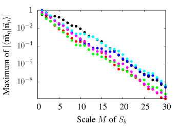
Figure 5: (Colored online) Demonstration for multi-Franck-Condon factor $\left|\langle\vec{\mathbf{n}}_{\mathsf{p}}|\vec{\mathbf{m}}_{\mathsf{q}}\rangle\right|$ by product from the maximal matrix elements of $|\langle n_{i}|\hat{D}(\Delta\alpha_{i,\mathsf{qp}}|m_{i}\rangle|$. The displacements are simulated by $M$ random number $\Delta\alpha_{i,\mathsf{qp}}\in(-4,4)$. We show 6 groups of samples, which decay exponentially with the system scale $M$.

Correspondingly, the master equation are obtained similarly to Eqs. (31, 32), and the thermalization rates for this composite system are

$$\Gamma_{\mathsf{p}\vec{\mathbf{n}},\mathsf{q}\vec{\mathbf{m}}}(\omega)=\begin{cases}\left|\langle\vec{\mathbf{n}}_{\mathsf{p}}|\vec{\mathbf{m}}_{\mathsf{q}}\rangle\right|^{2}J(\omega)N(\omega),&\omega\geq 0,\\ \left|\langle\vec{\mathbf{n}}_{\mathsf{p}}|\vec{\mathbf{m}}_{\mathsf{q}}\rangle\right|^{2}J(|\omega|)[N(|\omega|)+1],&\omega<0.\end{cases}$$

Comparing with the above case where $S_{b}$ only contains one harmonic oscillator, the only difference is that the thermalization rates are modified with a multi-Franck-Condon factor

$$\left|\langle\vec{\mathbf{n}}_{\mathsf{p}}|\vec{\mathbf{m}}_{\mathsf{q}}\rangle\right|^{2}=\prod_{i=1}^{M}\left|\langle n_{i,\mathsf{p}}|m_{i,\mathsf{q}}\rangle\right|^{2}.$$ (36)

Since each term in the product $\left|\langle n_{i,\mathsf{p}}|m_{i,\mathsf{q}}\rangle\right|^{2}<1$, when $M$ becomes large, the whole factor $\Gamma_{\mathsf{p}\vec{\mathbf{n}},\mathsf{q}\vec{\mathbf{m}}}(\omega)$ tends to vanish, and the thermalization rate approaches infinitesimal. That means, the speed of relaxation to the global thermal state is greatly suppressed by the multi-Franck-Condon factor due to the displacements of the Fock states when the degrees of freedom is large. We call this effect Franck-Condon blockade Koch and von Oppen (2005).

Here we estimate the maximum of the multi-Franck-Condon factor as,

$$\left|\langle\vec{\mathbf{n}}_{\mathsf{p}}|\vec{\mathbf{m}}_{\mathsf{q}}\rangle\right|^{2} \leq\prod_{i=1}^{M}\max_{\{m_{i},n_{i}\}}\Big{\{}\big{|}[\hat{D}(\Delta\alpha_{i,\mathsf{qp}})]_{m_{i},n_{i}}\big{|}^{2}\Big{\}}$$

$$\sim\exp[-M\langle\Delta\alpha_{i,\mathsf{qp}}^{2}\rangle]$$

where $\Delta\alpha_{i,\mathsf{qp}}:=\alpha_{i,\mathsf{q}}-\alpha_{i,\mathsf{p}}$. The above inequality achieves $1$ if and only if $\Delta\alpha_{i,\mathsf{qp}}=0$ for any $\mathsf{p},\,\mathsf{q},\,i$, namely, $\xi_{i,\mathsf{p}}\equiv\xi_{i}$ does not depend on $\mathsf{p}$ [Eq. (33)]. In this case the $N$-level system is indeed decoupled from the $M$ oscillators, and the interaction term only contributes displacements to the oscillators. The thermalization speed returns to the case for the thermalization of the $N$-level system alone, regardless of the $M$ oscillators. In usual cases, the multi-Franck-Condon factor gives rise to a exponential suppressing of the thermalization speed, which decays quite fast with the scale $M$ of the subsystem $S_{b}$ (Fig. 5).

VI Summary

In this paper, we have studied the synchro-thermalization for a composite system consisting of several subsystems, where only one of the subsystems is contacted with a canonical heat bath. It has been shown that the partial contact of one subsystem to the heat bath may stabilize the whole composite system to its canonical thermal state. We clarified that the conditions for the synchro-thermalization depends on the topology of the eigen-energy-level structure, i.e., whether it is connected or not. We illustrated our main results with an $N$-level system coupled to several harmonic oscillators via the non-demolition way.

Our arguments lead to a puzzle that the whole composite system can be thermalized even if the scale of the subsystems free of contact tends to be infinitely large. This puzzle can be explicitly solved by our illustration with the Franck-Condon blockade mechanism. When the degrees of freedom of the composite system becomes large, the thermalization rate would approach zero. That is to say, it becomes more and more difficult to stabilize the composite system to its canonical thermal state. Thus this effect of synchro-thermalization is not easy to be observed for large scale systems.

This work is supported by National Natural Science Foundation of China under Grants Nos. 11121403, 10935010 and 11074261, National 973-program Grants No. 2012CB922104, and Postdoctoral Science Foundation of China No. 2013M530516.

References

- Landau and Lifshitz (1980) L. Landau and E. Lifshitz, Statistical Physics, Part 1 (Butterworth-Heinemann, Oxford, 1980).
- Dong et al. (2007) H. Dong, S. Yang, X. F. Liu, and C. P. Sun, Phys. Rev. A 76, 044104 (2007).
- Dong et al. (2010) H. Dong, X. F. Liu, and C. P. Sun, Chin. Sci. Bull. 55, 3256 (2010), arXiv:0908.3997.
- Franck and Dymond (1926) J. Franck and E. G. Dymond, Trans. Faraday Soc. 21, 536 (1926).
- Condon (1926) E. Condon, Phys. Rev. 28, 1182 (1926).
- Lax (1952) M. Lax, J. Chem. Phys. 20, 1752 (1952).
- Koch and von Oppen (2005) J. Koch and F. von Oppen, Phys. Rev. Lett. 94, 206804 (2005).
- Breuer and Petruccione (2002) H. Breuer and F. Petruccione, The theory of open quantum systems (Oxford University Press, 2002).
- Kubo (1957) R. Kubo, J. Phys. Soc. Japan 12, 570 (1957).
- Martin and Schwinger (1959) P. C. Martin and J. Schwinger, Phys. Rev. 115, 1342 (1959).
- Le Bellac et al. (2004) M. Le Bellac, F. Mortessagne, and G. G. Batrouni, Equilibrium and non-equilibrium statistical thermodynamics (Cambridge University Press, 2004).
- Spohn (1977) H. Spohn, Lett. Math. Phys. 2, 33 (1977).
- Zhang et al. (2012) X.-J. Zhang, H. Qian, and M. Qian, Phys. Rep. 510, 1 (2012).
- Lupaşcu et al. (2007) A. Lupaşcu, S. Saito, T. Picot, P. C. de Groot, C. J. P. M. Harmans, and J. E. Mooij, Nature Phys. 3, 119 (2007).
- Schuster et al. (2007) D. I. Schuster, A. A. Houck, J. A. Schreier, A. Wallraff, J. M. Gambetta, A. Blais, L. Frunzio, J. Majer, B. Johnson, M. H. Devoret, S. M. Girvin, and R. J. Schoelkopf, Nature 445, 515 (2007).
- Brune et al. (1990) M. Brune, S. Haroche, V. Lefevre, J. M. Raimond, and N. Zagury, Phys. Rev. Lett. 65, 976 (1990).
- Caldeira and Leggett (1983) A. O. Caldeira and A. J. Leggett, Ann. Phys. 149, 374 (1983).