Mathematical Caricature of Large Waves.

Abstract

The Kadomtsev-Petviiashvili equation is considered as a mathematical caricature of large and rogue waves.

Large waves, also known as rogue, freak or monster waves, have been in marine folklore since the time immemorial inspiring awe and fear. Their description can be found in Greek, Scandinavian and Russian mythology, in 1887-1898 E. Rudolph, a professor of Geophysics of the University of Strasburg, Germany published over 600 pages on large waves and seaquakes documenting more than 550 drastic encounters of people with the sea. The stories of numerous sailors and sea men have inspired many an artist, e.g. Russian-Armenian artist Ivan Aivazovsky dedicated his famous painting ”Devyatiy Val” (translates from Russian as ”The ninth wall of water”) to such waves, Le Gray’s 1857 photograph ”The Great Wave” sold in 1999 for $838,000. Yet despite the overwhelming evidence the scientific establishment pretty much ignored large waves, any evidence presented was dismissed as un-scientific. Relatively recently scientific establishment admitted that monster waves exist and a deluge of research papers followed. The search for their explanation became so popular that any possible blow-up in a solution of an equation remotely related to waves is now called ”a rogue” or ”freak” wave and is considered to be an ”explanation” regardless of whether it has anything to do with such waves or not.

In this talk we will look at large waves through the mirror of the Kadomtsev-Petviashvili equation. As pretty much any mathematical model the Kadomtsev-Petviashvili equation may be compared to a curved mirror. A small fly flying by the mirror will see an almost perfect reflection of itself but the reflections of much larger buildings will be quite distorted. Yet despite the distortion the latter will show windows, floors, etc. of the buildings. Similarly the Kadomtsev-Petviashvili equation provides a good description of soliton walls but only a distorted description of larger waves; however, despite the distortion the appropriately chosen solutions of the Kadomtsev-Petviashvili equation show us some features of large waves. It would be nice to have a better mathematical model but as Albert Einstein once said, ”As far as the laws of mathematics refer to reality, they are not certain; and as far as they are certain, they do not refer to reality ”.

To derive the Kadomtsev-Petviashvili equation in physical coordinates $x^{\prime},y^{\prime},z^{\prime},t^{\prime}$ we assume that the motion of fluid is restricted to the region $-h<z^{\prime}<\epsilon h\eta(x^{\prime},y^{\prime},t^{\prime})$, where $z^{\prime}=\epsilon h\eta(x^{\prime},y^{\prime},t^{\prime})$ is the elevation of the free surface, $h>0,\;0<\epsilon\ll 1$ are constants. The velocity of fluid $\mathbf{u^{\prime}}$ has a potential

$\epsilon\phi$, i.e. $\mathbf{u^{\prime}}=\epsilon\nabla\phi.$ In dimensionless variables $T=t^{\prime}\sqrt{\frac{\epsilon^{3}g}{h}},\;X=\sqrt{\epsilon}\frac{x^{\prime}-t^{\prime}\sqrt{gh}}{h},\;Y={\epsilon}\frac{y^{\prime}}{h},\;Z=\frac{z^{\prime}}{h},\;\Phi=\phi\sqrt{\frac{\epsilon}{gh^{3}}},\;S=\frac{s}{\rho h^{2}g},$ the equations of motion take form

$$\epsilon\frac{\partial^{2}\Phi}{\partial X^{2}}+\epsilon^{2}\frac{\partial^{2}\Phi}{\partial Y^{2}}+\frac{\partial^{2}\Phi}{\partial Z^{2}}=0\hskip 99.58464pt\text{ in }-1<Z<\epsilon\eta,$$

$$\frac{\partial\Phi}{\partial Z}=0\hskip 204.85983pt\mbox{ on }Z=-1,$$

$$\dfrac{\partial\Phi}{\partial Z}=-\epsilon\dfrac{\partial\eta}{\partial X}+\epsilon^{2}\dfrac{\partial\eta}{\partial T}+\epsilon^{2}\dfrac{\partial\Phi}{\partial X}\dfrac{\partial\eta}{\partial X}+\epsilon^{3}\dfrac{\partial\Phi}{\partial Y}\dfrac{\partial\eta}{\partial Y}\hskip 36.98857pt\mbox{ on }Z=\epsilon\eta,$$

$$\eta-S\epsilon\eta_{XX}-S\epsilon^{2}\eta_{YY}-\tfrac{\partial\Phi}{\partial X}+\epsilon\tfrac{\partial\Phi}{\partial T}+\tfrac{1}{2}\left(\tfrac{\partial\Phi}{\partial Z}\right)^{2}+\tfrac{1}{2}\epsilon\left(\tfrac{\partial\Phi}{\partial X}\right)^{2}+\tfrac{1}{2}\epsilon^{2}\left(\tfrac{\partial\Phi}{\partial Y}\right)^{2}=0\mbox{ on }Z=\epsilon\eta,$$

with details of the derivation elaborated in [Kov 1].

Solutions are sought in the form $\Phi=\Phi_{0}+\epsilon\Phi_{1}+\epsilon^{2}\Phi_{2}+\dots,\newline \;\;\eta=\eta_{0}+\epsilon\eta_{1}+\dots,$ which upon substitution in the equations of motion yield

$$\dfrac{\partial}{\partial x^{\prime}}\left[\dfrac{1}{\sqrt{gh}}\;\eta_{0t^{\prime}}+\eta_{0x^{\prime}}+\dfrac{\rho gh^{2}-3S}{6\rho g}\eta_{0x^{\prime}x^{\prime}x^{\prime}}+\dfrac{3\epsilon}{2}\eta_{0}\eta_{0x^{\prime}}\right]+\dfrac{1}{2}\eta_{0y^{\prime}y^{\prime}}=0,$$

$$u^{\prime}_{x^{\prime}}\hskip-2.84526pt=\hskip-2.84526pt\epsilon\sqrt{gh}\;\eta_{0}+o(\epsilon),\;\;u^{\prime}_{z^{\prime}}\hskip-2.84526pt=\hskip-2.84526pt-\epsilon(h+z^{\prime})\sqrt{gh}\;\dfrac{\partial\eta_{0}}{\partial x^{\prime}}+o\left(\epsilon^{3/2}\right).$$

Change of variables $\alpha^{2}=\dfrac{2\rho g}{\rho gh^{2}-3S},\;t^{\prime}=\dfrac{3\alpha^{2}\;t}{\sqrt{gh}},x^{\prime}=x+{3\alpha^{2}}t,\;y^{\prime}=\dfrac{y}{\sqrt{2}\thinspace},\;\eta_{0}=\dfrac{4f}{3\epsilon\alpha^{2}},$ simplifies the latter equations to

$$\dfrac{\partial}{\partial x}\Big{[}f_{t}+f_{xxx}+6ff_{x}\Big{]}+3\alpha^{2}f_{yy}=0,\quad\alpha^{2}=\pm 1,$$

known as the Kadomtsev-Petviashvili equation or simply KP and

$$u^{\prime}_{x^{\prime}}\hskip-2.84526pt=\hskip-2.84526pt\;\dfrac{4\sqrt{gh}}{3\alpha^{2}}f+o(\epsilon),\;\;u^{\prime}_{z^{\prime}}\hskip-2.84526pt=\hskip-2.84526pt-(h+z^{\prime})\;\dfrac{4\sqrt{gh}}{3\alpha^{2}}\dfrac{\partial f}{\partial x^{\prime}}+o\left(\epsilon^{3/2}\right),$$

which we call the velocity conditions. The latter are often ignored yet, as will see later, they play fundamental role in the explanation of rogue waves.

The simplest solutions of KP are the so-called multi-soliton solutions

$$f(x,y,t)=2\frac{\partial^{2}}{\partial x^{2}}\ln\det{\boldsymbol{A}},$$

where $\displaystyle{\boldsymbol{A}}_{mn}=\delta_{mn}+\frac{c_{n}\enskip e^{(p_{n}+q_{n})x+(q_{n}^{2}-p_{n}^{2})y-(p_{n}+q_{n})\big{[}(p_{n}+q_{n})^{2}+3\alpha^{2}(p_{n}-q_{n})^{2}\big{]}t}}{p_{n}+q_{m}},$ $m,n=1\dots N,\delta_{mn}$ are the regular Kronecker symbols, $c_{n},\;p_{n},\;q_{n}$ are real constants. Numerous illustrations of soliton and multi-soliton waves are available on the Internet.

If we take nonlinear superposition of 2N solitons with $p_{2k-1}={\overline{p_{2k}}}=i\lambda_{k}+\mu_{k}+\varepsilon e^{i\chi_{n}},\;q_{2k-1}={\overline{q_{2k}}}=i\lambda_{k}-\mu_{k}+\varepsilon e^{-i\chi_{n}},\;c_{2k-1}={\overline{c_{2k}}}=2\varepsilon e^{i\gamma_{k}-i\chi_{n}+\varrho_{k}\varepsilon},\;\lambda_{k},\mu_{k},\gamma_{k},\varrho_{k}\in{R},$ $\;k=1\dots N$ and let $\epsilon\to 0$ we obtain

$$u(x,y,t)=2\frac{\partial^{2}}{\partial x^{2}}\ln\det{\boldsymbol{K}},$$

where $\;\;{\boldsymbol{K}}=\left(\begin{array}[]{ccccc}K_{11}&K_{12}&\dots&K_{1N}\\ K_{21}&K_{22}&\dots&K_{2N}\\ \vdots&\vdots&\vdots&\vdots\\ K_{N1}&K_{N2}&\dots&K_{NN}\end{array}\right);\hskip 14.22636ptK_{nn}=\Upsilon_{n}-\dfrac{\sin 2\Gamma_{n}}{2\lambda_{n}};\hskip 14.22636pt\text{ for }n\neq k\hskip 11.38109ptK_{nk}=\left[\dfrac{(\lambda_{n}-\lambda_{k})\sin(\Gamma_{n}-\Gamma_{k})}{\alpha^{2}(\mu_{n}-\mu_{k})^{2}+(\lambda_{n}-\lambda_{k})^{2}}-\right.\newline \left.\dfrac{(\lambda_{n}+\lambda_{k})\sin(\Gamma_{n}+\Gamma_{k})}{\alpha^{2}(\mu_{n}-\mu_{k})^{2}+(\lambda_{n}+\lambda_{k})^{2}}\right]+\alpha\left[\dfrac{(\mu_{n}-\mu_{k})\cos(\Gamma_{n}+\Gamma_{k})}{\alpha^{2}(\mu_{n}-\mu_{k})^{2}+(\lambda_{n}+\lambda_{k})^{2}}-\dfrac{(\mu_{n}-\mu_{k})\cos(\Gamma_{n}-\Gamma_{k})}{\alpha^{2}(\mu_{n}-\mu_{k})^{2}+(\lambda_{n}-\lambda_{k})^{2}}\right];\hskip 14.22636pt\Gamma_{n}=\gamma_{n}+\lambda_{n}x-2\lambda_{n}\mu_{n}y+4\lambda_{n}(\lambda_{n}^{2}-3\alpha^{2}\mu_{n}^{2})t;\hskip 14.22636pt\Upsilon_{n}=\rho_{n}+x\cos(\alpha\chi_{n})+2\left[\dfrac{\lambda_{n}\sin(\alpha\chi_{n})}{\alpha}-\mu_{n}\cos(\alpha\chi_{n})\right]y+12\Big{[}\lambda_{n}^{2}\cos(\alpha\chi_{n})-\alpha^{2}\mu_{n}^{2}\cos(\alpha\chi_{n})+2\alpha\lambda_{n}\mu_{n}\sin(\alpha\chi_{n})\Big{]}t;\hskip 14.22636pt\lambda_{n}\textmd{{'s, }}\mu_{n}\textmd{'s, }\chi_{n}\textmd{'s, }\gamma_{n}\textmd{'s, }\rho_{n}\textmd{'s }$ are constants.

For $N=1$ formulas (1) degenerate into

$$f(x,y,t)=2\displaystyle\frac{\partial^{2}}{\partial x^{2}}\ln\Big{[}2\lambda\Upsilon-{\sin 2\Gamma}\Big{]},$$

where $\displaystyle\Gamma=\gamma+\lambda x-2\lambda\mu y+4\lambda(\lambda^{2}-3\alpha^{2}\mu^{2})t;\hskip 14.22636pt\Upsilon=\rho+x\cos(\alpha\chi)+2\Bigg{[}\dfrac{\lambda\sin(\alpha\chi)}{\alpha}-\mu\cos(\alpha\chi)\Bigg{]}y+12\Big{[}\lambda^{2}\cos(\alpha\chi)-\alpha^{2}\mu^{2}\cos(\alpha\chi)+2\alpha\lambda\mu\sin(\alpha\chi)\Big{]}t;\hskip 14.22636pt\lambda,\mu,\chi,\gamma,\rho$ are constants. We shall refer to (2) as a harmonic breather for reasons discussed in [Kov 2], formula (1) may be viewed as nonlinear superposition of harmonic breathers.

Solution (2) of KP is singular and approaches $-\infty$ as we move towards the singular curve $2\lambda\Upsilon-{\sin 2\Gamma}=0.$ To be physically plausible it needs to be regularized to remove infinities; since there is no clear way to determine what kind of regularization is most suitable we choose an ad-hoc regularization

$$f\to F=\displaystyle\frac{f}{|f|}\ln\Big{[}\ln\Big{(}\Big{|}e^{f}-1\Big{|}+1\Big{)}+1\Big{]}$$

due to its properties $F\approx f,\textmd{ if }0<|f|\ll 1;\;\;\;F=0,\textmd{ if }f=0;\;\;\;F\to-\ln(\ln 2+1),\textmd{ as }f\to-\infty;\;\;\;F\approx\ln f\textmd{ as }f\to+\infty.$ The regularization is close to the original function for $|f|\ll 1,$ removes negative infinity and reduces large amplitudes to make them more

physically plausible.

Regularization of harmonic breather (2) with $\chi=0$ is shown in Figure 1. Harmonic breather (2) with $\chi=0$ is divided into two simply connected components by a singular line suggesting that each component might describe a separate physical wave, regularization of one such half is shown in Figure 2. The physical waves described, albeit imperfectly, by such simply connected components are known as undular bores, a few examples are shown in Figures 3-6; more pictures of undular bores can be found on the Internet.

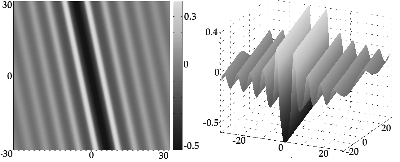
Figure 1: Graph of regularization (3) of (2) with $\alpha\hskip-1.42262pt=\hskip-1.42262pt1,\;\lambda\hskip-1.42262pt=\hskip-1.42262pt0.5,\;\mu\hskip-1.42262pt=\hskip-1.42262pt-0.1,\;\gamma\hskip-1.42262pt=\hskip-1.42262pt0,\rho\hskip-1.42262pt=\hskip-1.42262pt0,\;\chi\hskip-1.42262pt=\hskip-1.42262pt0,\;t\hskip-1.42262pt=\hskip-1.42262pt0.$

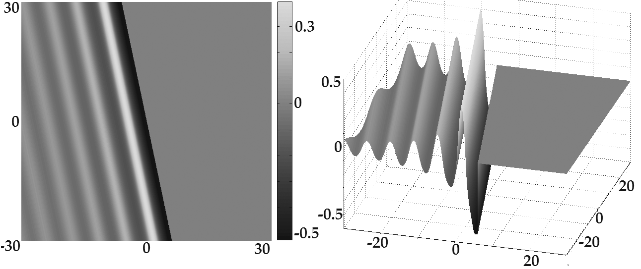
Figure 2: Graph of regularization (3) of a simply connected half of (2) with $\alpha\hskip-1.42262pt=\hskip-1.42262pt1,\;\lambda\hskip-1.42262pt=\hskip-1.42262pt0.5,\;\mu\hskip-1.42262pt=\hskip-1.42262pt-0.1,\;\gamma\hskip-1.42262pt=\hskip-1.42262pt0,\rho\hskip-1.42262pt=\hskip-1.42262pt0,\;\chi\hskip-1.42262pt=\hskip-1.42262pt0,\;t\hskip-1.42262pt=\hskip-1.42262pt0.$ The plot is discontinuous along the straight line $2\lambda\Upsilon-{\sin 2\Gamma}=0$, however Matlab replaced the discontinuity with a vertical strip and the author decided to leave it that way.

Figure 3: An undular bore generated by tide on the Garonne river at Arcins on July 6, 2008 around 07:10 views from right bank. Courtesy of Hubert Chanson.

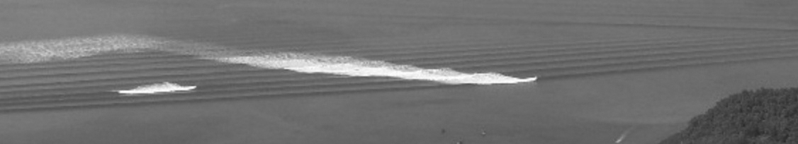
Figure 4: An undular bore generated by the tsunami of December 26, 2004 approaching Koh Jum island, off the coast of Thailand, after it passed around the Phi Phi islands. Copyright Anders Grawin, 2006. Reproduced from http://www.kohjumonline.com/anders.html with permission.

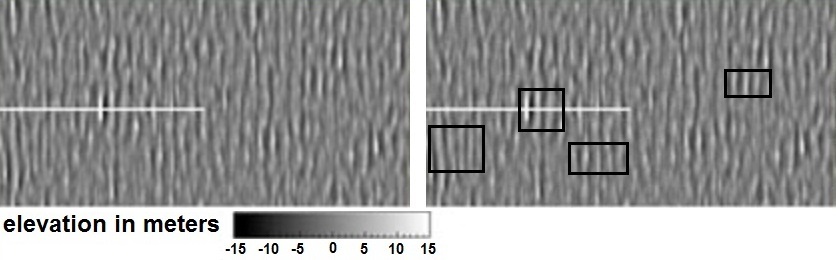
Figure 5: Image captured by ESA, courtesy of ESA and Deutsches Zentrum fur Luft- und Raumfahrt (DLR). On the left is the original image, on the right is the same image with some waves of the type shown in Figures 1 and 2 enclosed in black rectangles. The middle of the horizontal white line marks the wave with the highest crest, it is the leading crest of a wave of the type shown in Figure 2. Reproduced with permission.

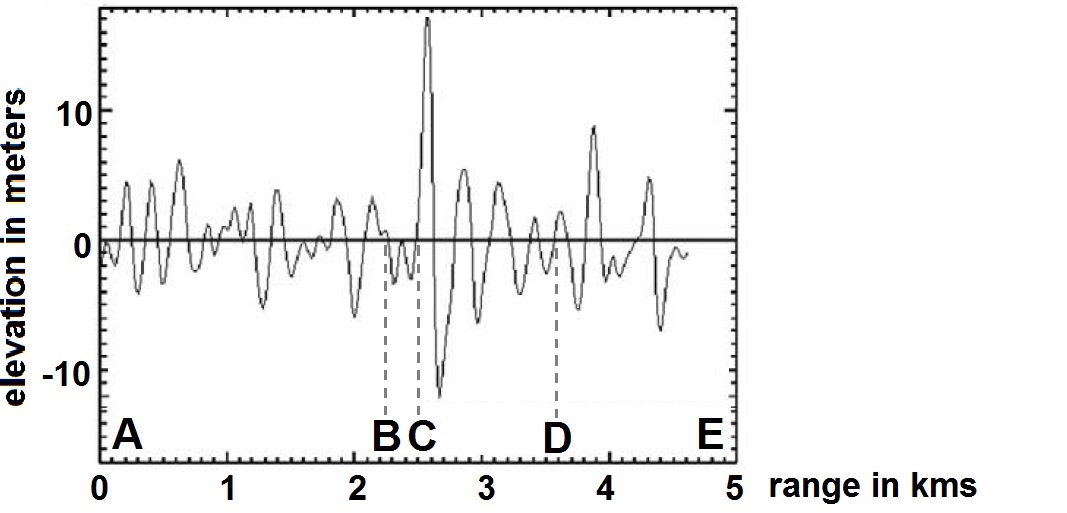
Figure 6: The vertical transect of the previous picture along the straight white line. Region CD is as predicted by the formula, region BC corresponds to the negative singularity. In regions AB and DE the undular bore-like behavior is masked by other waves. Reproduced with permission.

Typical undular bore exhibits non-smooth behavior at the leading front reflected by the presence of a singularity in the solution. Formulas (VC) imply wave overturning, large acceleration and thus the presence of large forces at the leading front/trough; description of the power of undular bores near the leading front/trough is given in Wolanski, E., Williams, D., Spagnol, S., and Chanson, H. (2004), Undular Tidal Bore Dynamics in the Daly Estuary, Northern Australia. Estuarine, Coastal and Shelf Science, Vol. 60, No. 4, pp. 629-636 (DOI: 10.1016/j.ecss.2004.03.001) , ” This unsteady motion was sufficiently energetic to topple moorings that had survived much higher, quasi-steady currents of 1.8 m/s”

Regularization of harmonic breather (2) with $\chi\neq 0$ is shown in Figure 7 while physical waves described, albeit imperfectly, by such waves are shown in Figures 8-9.

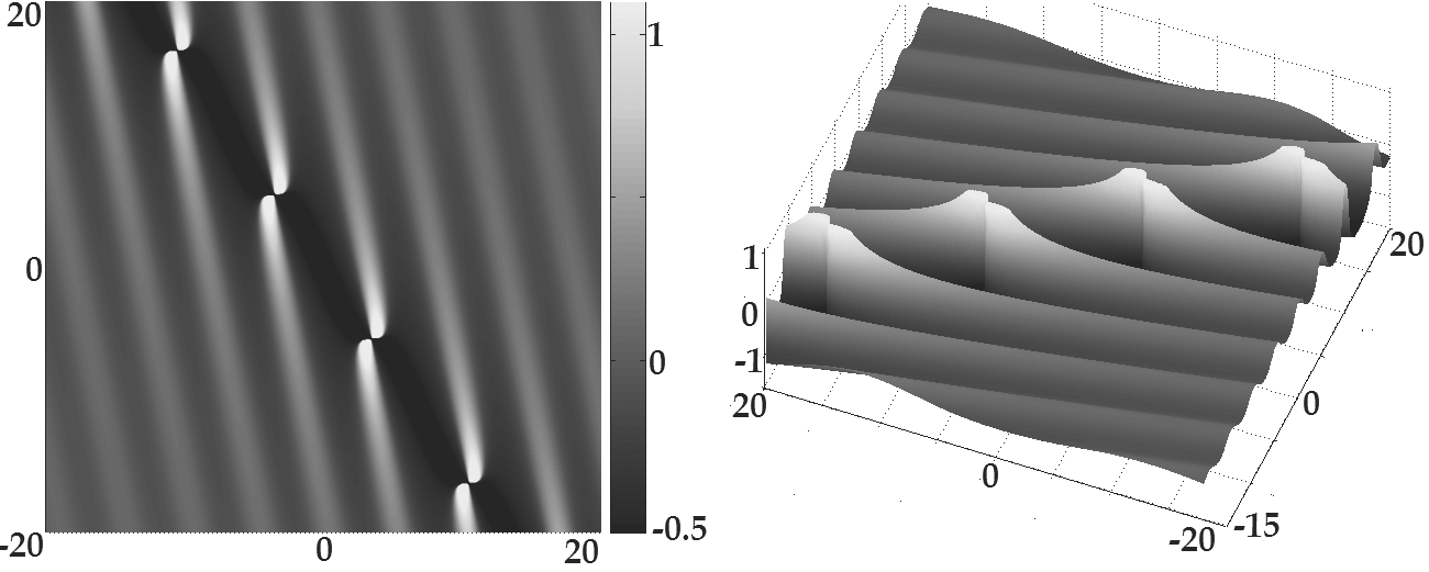
Figure 7: Graph of regularization (3) of (2) with $\alpha\hskip-1.5649pt=\hskip-1.5649pt1,\lambda\hskip-1.5649pt=\hskip-1.5649pt0.65,\mu\hskip-1.5649pt=\hskip-1.5649pt-0.1,\gamma\hskip-1.5649pt=\hskip-1.5649pt0,\rho\hskip-1.5649pt=\hskip-1.5649pt0,\chi\hskip-1.5649pt=\hskip-1.5649pt.105\pi,t\hskip-1.5649pt=\hskip-1.5649pt0.$

Figure 8: Portion of time frame t = 2 : 11 from the video at [Rip Curl] depicts a wave on the river of Seven Ghosts, Indonesia. The shape of the wave is in agreement with Figure 2 with $\chi$ close to but not equal to zero except for wave overturning exhibited by the physical wave shown but not by Figure 7. Reproduced with permission.

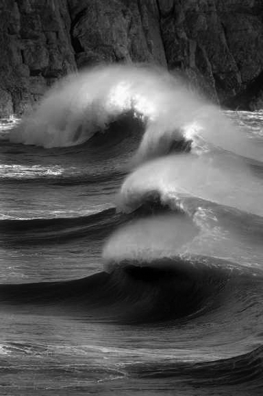
Figure 9: The shape of this wave at Hells Mouth, Wales, is in agreement with Figure 2 with $\chi\neq 0$ except for wave overturning exhibited by the physical wave shown but not by Figure 7. The photograph is reproduced from http://magicseaweed.com/photoLab/viewPhoto.php?photoId=18664 , courtesy of John Wormald.

Harmonic breather (2) with $\chi\neq 0$ is divided into two simply connected by the singular curve suggesting that each simply connected component might describe a separate physical wave, regularization of one such component is shown in Figure 10 while a corresponding physical wave is shown in Figure 11.

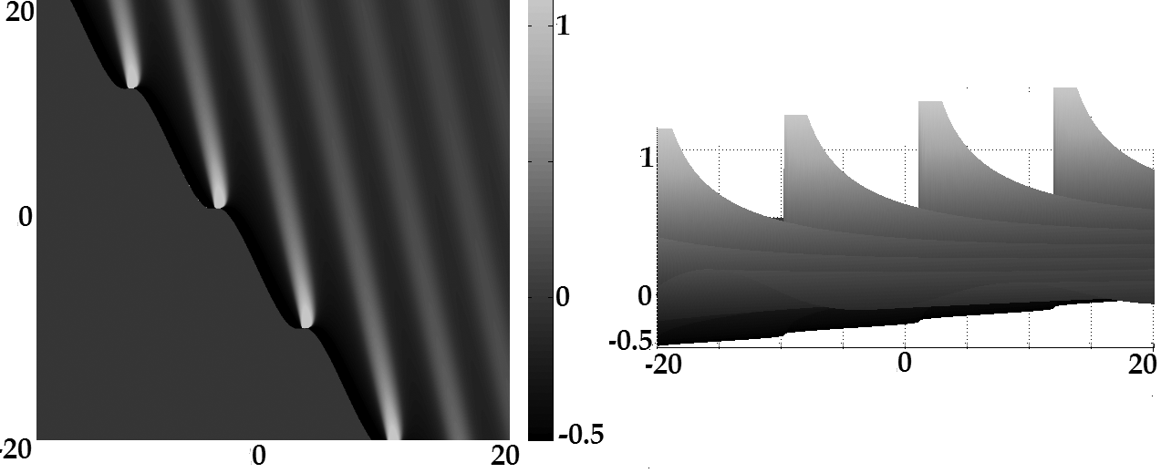
Figure 10: Graph of regularization (3) of a simply connected component of (2) with $\alpha\hskip-1.42262pt=\hskip-1.42262pt1,\;\lambda\hskip-1.42262pt=\hskip-1.42262pt0.65,\;\mu\hskip-1.42262pt=\hskip-1.42262pt-0.1,\;\gamma\hskip-1.42262pt=\hskip-1.42262pt0,\rho\hskip-1.42262pt=\hskip-1.42262pt0,\;\chi\hskip-1.42262pt=\hskip-1.42262pt0.105\pi,\;t\hskip-1.42262pt=\hskip-1.42262pt0.7.$

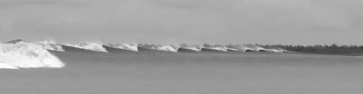
Figure 11: Portion of time frame t =1:17 from the video at [Rip Curl] depicts a wave on the river of Seven Ghosts, Indonesia, its shape is in agreement with Figure 10 with $\chi\neq 0$ except for wave overturning exhibited by the physical wave shown but not by Figure 10. Reproduced with permission.

If the spectral parameters $\lambda,\mu$ are sufficiently large the graph of the regularization of a harmonic breather with $\chi\neq 0$ is shown in Figure 12 while a corresponding physical wave is shown in Figure 13.

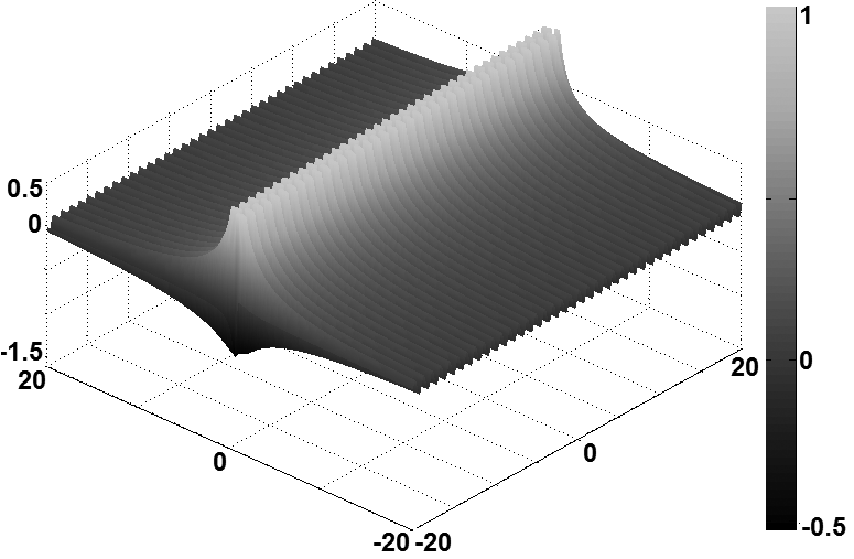
Figure 12: Graph of regularization (3) of (2) with $\alpha\hskip-1.42262pt=\hskip-1.42262pt1,\;\lambda\hskip-1.42262pt=\hskip-1.42262pt3,\;\mu\hskip-1.42262pt=\hskip-1.42262pt0,\;\gamma\hskip-1.42262pt=\hskip-1.42262pt0,\rho\hskip-1.42262pt=\hskip-1.42262pt0,\;\chi\hskip-1.42262pt=\hskip-1.42262pt0.55\pi,\;t\hskip-1.42262pt=\hskip-1.42262pt0.$

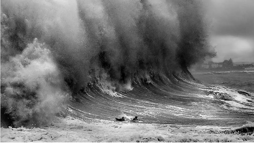
Figure 13: A physical wave with the shape predicted by Figure 12. Notice the streaks across the wave and a ”cloud” of droplets. Compare it to the wave shown in Figure 16. Reproduced from public domain http://mpora.com/photos/T5SsfsQ7BR .

Another class of explicit solutions of KP is obtained by substitution $\lambda_{k}\to i\lambda_{k},\;\chi_{k}\to i\chi_{k},\;\gamma_{k}\to i\gamma_{k}$ into formulas (1) and (2) yielding correspondingly

$$u(x,y,t)=2\frac{\partial^{2}}{\partial x^{2}}\ln\det{\boldsymbol{K}}$$

where ${\boldsymbol{K}}=\left(\begin{array}[]{llll}K_{11}&K_{12}&\dots&K_{1N}\\ K_{21}&K_{22}&\dots&K_{2N}\\ \vdots&\vdots&\vdots&\vdots\\ K_{N1}&K_{N2}&\dots&K_{NN}\end{array}\right);\hskip 14.22636ptK_{nn}=\Upsilon_{n}-\dfrac{\sinh 2\Gamma_{n}}{2\lambda_{n}};\hskip 14.22636pt\text{ for }n\neq k\hskip 8.53581ptK_{nk}=\left[-\dfrac{(\lambda_{n}-\lambda_{k})\sinh(\Gamma_{n}-\Gamma_{k})}{\alpha^{2}(\mu_{n}-\mu_{k})^{2}-(\lambda_{n}-\lambda_{k})^{2}}\right.\newline \left.+\dfrac{(\lambda_{n}+\lambda_{k})\sinh(\Gamma_{n}+\Gamma_{k})}{\alpha^{2}(\mu_{n}-\mu_{k})^{2}-(\lambda_{n}+\lambda_{k})^{2}}\right]+\alpha\left[\dfrac{(\mu_{n}-\mu_{k})\cosh(\Gamma_{n}+\Gamma_{k})}{\alpha^{2}(\mu_{n}-\mu_{k})^{2}-(\lambda_{n}+\lambda_{k})^{2}}-\dfrac{(\mu_{n}-\mu_{k})\cosh(\Gamma_{n}-\Gamma_{k})}{\alpha^{2}(\mu_{n}-\mu_{k})^{2}-(\lambda_{n}-\lambda_{k})^{2}}\right];\hskip 14.22636pt\Gamma_{n}=\gamma_{n}+\lambda_{n}x-2\lambda_{n}\mu_{n}y-4\lambda_{n}(\lambda_{n}^{2}+3\alpha^{2}\mu_{n}^{2})t;\hskip 14.22636pt\Upsilon_{n}=\rho_{n}+x\cosh(\alpha\chi_{n})-2\Big{[}\displaystyle\frac{\lambda_{n}\sinh(\alpha\chi_{n})}{\alpha}+\mu_{n}\cosh(\alpha\chi_{n})\Big{]}y-12\Big{[}\lambda_{n}^{2}\cosh(\alpha\chi_{n})+\alpha^{2}\mu_{n}^{2}\cosh(\alpha\chi_{n})\newline +2\alpha\lambda_{n}\mu_{n}\sinh(\alpha\chi_{n})\Big{]}t;\hskip 14.22636pt\lambda_{n}\textmd{'s, }\mu_{n}\textmd{'s, }\chi_{n}\textmd{'s, }\gamma_{n}\textmd{'s, }\rho_{n}\textmd{'s }$ are constants.

For $N=1$ formulas (4) degenerate to

$$f(x,y,t)=2\displaystyle\frac{\partial^{2}}{\partial x^{2}}\ln\Big{[}2\lambda\Upsilon-{\sinh 2\Gamma}\Big{]},$$

where $\Gamma=\gamma+\lambda x-2\lambda\mu y-4\lambda(\lambda^{2}+3\alpha^{2}\mu^{2})t;\hskip 14.22636pt\Upsilon=\rho+x\cosh(\alpha\chi)-2\Bigg{[}\dfrac{\lambda\sinh(\alpha\chi)}{\alpha}+\mu\cosh(\alpha\chi)\Bigg{]}gy-12\Big{[}\lambda^{2}\cosh(\alpha\chi)+\alpha^{2}\mu^{2}\cosh(\alpha\chi)+2\alpha\lambda\mu\sinh(\alpha\chi)\Big{]}t;\hskip 8.53581pt\lambda,\mu,\chi,\gamma,\rho$ are constants. We shall refer to (5) as solitonic dipole for reasons discussed in [Kov 2]. Regularization of a solitonic dipole (5) with $\chi\neq 0$ is shown in Figure 14. We can also take a half-wave as before although now we cut it in half in the middle not along the singular curve. Physical analogues of such waves are shown in Figures 16-18, more illustrations of physical waves described by solitonic dipoles may be found on the Internet.

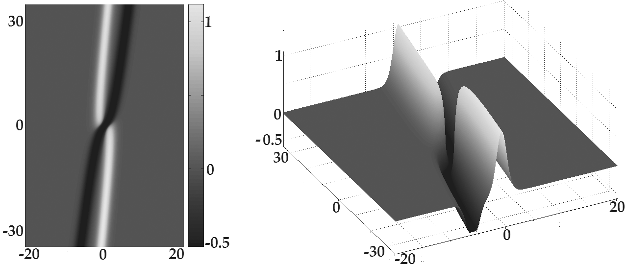
Figure 14: Graph of regularization (3) of (5) with $\alpha\hskip-1.42262pt=\hskip-1.42262pt1,\,\lambda\hskip-1.42262pt=\hskip-1.42262pt1,\,\mu\hskip-1.42262pt=\hskip-1.42262pt0.05,\,\gamma\hskip-1.42262pt=\hskip-1.42262pt0,\,\rho\hskip-1.42262pt=\hskip-1.42262pt0,\,\chi\hskip-1.42262pt=\hskip-1.42262pt0.6,\,t\hskip-1.42262pt=\hskip-1.42262pt0.$

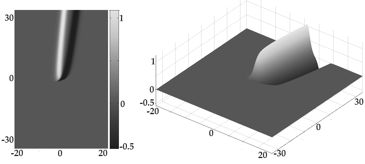
Figure 15: Graph of regularization (3) of the upper half of (5) with $\alpha\hskip-1.42262pt=\hskip-1.42262pt1,\,\lambda\hskip-1.42262pt=\hskip-1.42262pt1,\,\mu\hskip-1.42262pt=\hskip-1.42262pt0.05,\,\gamma\hskip-1.42262pt=\hskip-1.42262pt0,\,\rho\hskip-1.42262pt=\hskip-1.42262pt0,\,\chi\hskip-1.42262pt=\hskip-1.42262pt0.6,\,t\hskip-1.42262pt=\hskip-1.42262pt0.\hskip 312.9803pt$

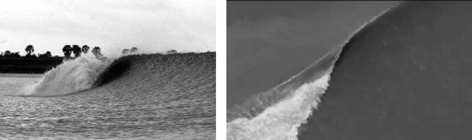
Figure 16: On the left is a tidal bore in the Amazon River; with the height reaching up to 4 meters it travels as much as 13 kilometers inland upstream from the Atlantic Ocean in February and March. Reproduced from public domain http://captainkaisworld.blogspot.ca/2011/04/surfing-rivers-7-ghosts-severn-chinas.html . On the right is a portion of time frame t =0:52 from the video at [Rip Curl] depicting a wave on the river of Seven Ghosts, Indonesia. Unlike the wave shown in Figure 13 these waves do not have strongly defined transverse streaks or the ”cloud” of droplets above it, the crest is relatively well-defined compared to Figure 13. Reproduced with permission.

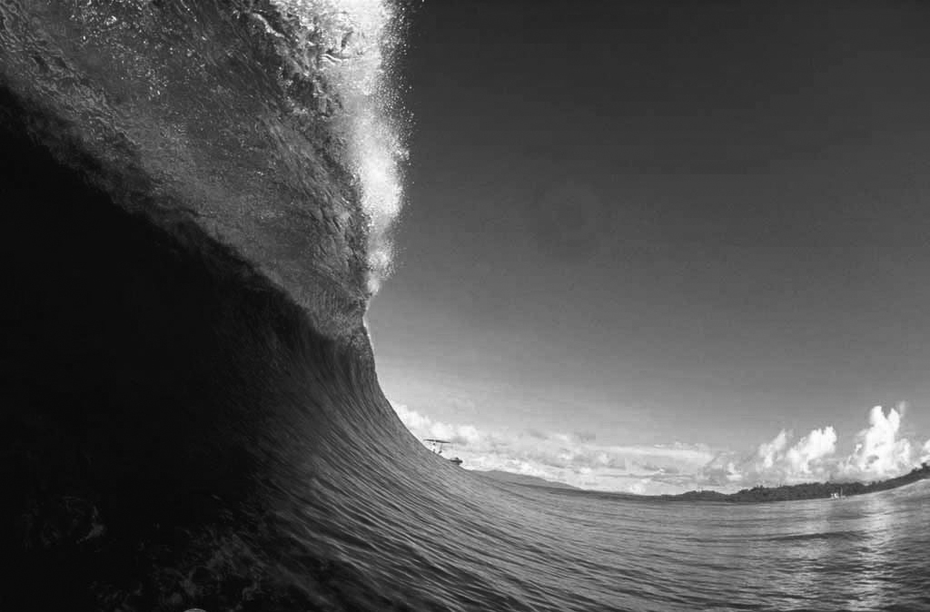
Figure 17: The picture emphasizes the trough rather than the crest of the wave. Reproduced from a public web site, due to numerous web sites showing this picture the origin is unknown.

Figure 18: Image captured by ESA, courtesy of ESA and Deutsches Zentrum fur Luft- und Raumfahrt (DLR). On the left is the original image, on the right is the same image with some half-waves shown in black rectangles and two full waves shown in white rectangles. Reproduced with permission.

The waves discussed have relatively long life-span, yet there are accounts of extremely powerful waves that appear seemingly out of nowhere and disappear shortly thereafter into nowhere. Remarkably, KP predicts the existence of such waves and provides their explanation. Let us look at Figure 19 showing $\widetilde{f}(x,y,t)=\left\{\begin{array}[]{l}\displaystyle\frac{f}{|f|}\ln\Big{[}\ln\Big{(}\Big{|}e^{f}-1\Big{|}+1\Big{)}+1\Big{]},\textmd{ if }f\leqslant 0,\\ \\ \max\{f,10\},\textmd{ if }f>0,\end{array}\right.,$ where $f$ is nonlinear superposition of two solitonic dipoles given by (4); it illustrates the creation of a short-lived physically localized rogue wave seemingly out of nowhere. The physics behind it is shown in Figure 20.

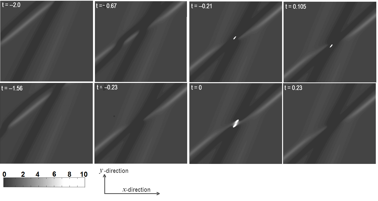
Figure 19: Time evolution of $\widetilde{f}$ where $f$ is given by (4) with $N\hskip-2.84526pt=\hskip-2.84526pt2,\,\alpha\hskip-2.84526pt=\hskip-2.84526pt1,\chi_{1}\hskip-2.84526pt=0.6,\,\lambda_{1}\hskip-2.84526pt=0.5,\,\mu_{1}\hskip-2.84526pt=0.2,\,\gamma_{1}\hskip-2.84526pt=0,\,\rho_{1}\hskip-2.84526pt=0,\,\chi_{2}\hskip-2.84526pt=\hskip-2.84526pt-0.7,\,\lambda_{2}\hskip-2.84526pt=1,\,\mu_{2}\hskip-2.84526pt=0.5,\,\gamma_{2}\hskip-2.84526pt=0,\,\rho_{2}\hskip-2.84526pt=0$ in the region $-15<x,y<15$. Notice the rogue wave shown by white spots near the center; it is short-lived and exists only for t close to 0.

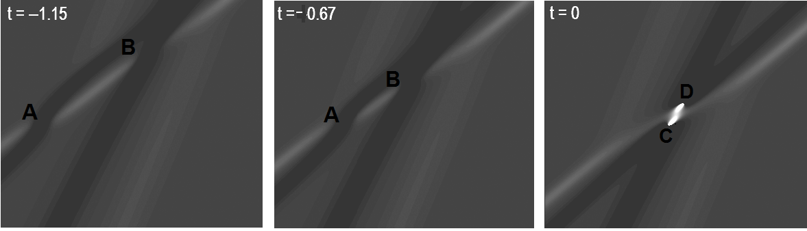
Figure 20: Function of Figure 19 at $t=-1.15,\;t=-0.67,\;t=0.$ According to (VC) water in the white regions moves to the right while at the dark regions it moves to the left thus creating undertow currents at points A and B. As $t\to 0^{-}$ points A and B move so close to each other that the flow of water from each current gets in the way of the flow in the other current, the two colliding flows have no other way to go but up creating a rogue wave. Once $t$ passes $0$ points A and B move away from each other and the rogue wave disappears. The rogue wave is short-lived, it exists only for $t$ close to $0$. Notice that the rogue wave appearing at $t=0$ has two tops at points C and D.

There is a remarkable similarity of the predictions of Figures 19-20 to the Aivasovsky’s painting ”Devyatiy Val” . The column of water is large and does not break at $t=0$ only for certain values of the angle between the two troughs, the parameters in Figures 19-20 are chosen to produce an appropriate angle. The angle between the troughs shown in the Aivasovsky’s painting ”Devyatiy Val” is very close to the angle between the troughs in Figures 19-20. The rogue wave rises up at the intersection of the two troughs both in Figures 19-20 and in the painting. Is the similarity merely coincidental or the result of Aivasovsky’s numerous discussions with sailors and sea men who undoubtedly had encountered rogue waves? The answer to this question we will never know.

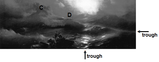
Figure 21: Lower half of ”Devyatiy Val” by Aivasovsky. Notice that the two troughs intersect at the angle about the same as the angle of intersection of the troughs in Figures 19,20 at $t=0$. The rogue wave in the painting has two tops at points C and D, and so does the rogue wave in Figures 19 and 20 at $t=0$. In the painting the top at D is overturning. The line connecting points C and D is almost parallel to one of the troughs both in Figures 19, 20 and in the painting. Reproduced from public domain http://thewallpapers.co.uk/?s=Aivazovsky%20-%20The%20Ninth%20Wave&page=1 .

Here we have shortly discussed modeling large waves with the solutions of KP, the topic is elaborated in [Kov 1]. The modeling is more of qualitative than quantitive nature and is far from perfect. Such models are often called mathematical caricatures since just like ordinary caricatures they capture only certain important aspects of the original while loosing or distorting others. Despite its imperfections KP has one advantage over many other models including the nonlinear Schrodinger equation, and that is its two dimensionality as to properly describe large waves one needs two space dimensions. Models with only one space dimension may be popular and fruitful (in terms of the number of publications one can produce using such models) but completely irrelevant as far as the physical waves are concerned.