Polarization vortex domains induced by switching electric field in ferroelectric films with circular electrodes

Abstract

We describe ferroelectric thin films with circular electrodes and develop a thermodynamic theory that explains exotic experimental results previously reported. It is found to be especially useful for restricted geometries such as microstructures for which boundary conditions are well known to play an important role in ferroelectric properties. We have explored a new switching mechanism, which consists of an inhomogeneous rotational motion of the polarization and leads to an vortex state. The vortex appearance exhibits characteristic properties of a first-order field-induced phase transition with three critical electric fields and the possibility of hysteresis behavior.

I INTRODUCTION

The knowledge of spatial distribution of polarization in thin and ultra-thin ferroelectric films is very important for their evaluation for device applications. In fact, the finite-size ferroelectric samples exhibit properties that are different from those for bulk materials DAWBER_2005 . Description of the nonuniform distribution of ferrelectric polarizaration in frame of phase transition theory with suitable boundary conditions has been successfully used to investigate the thin films properties TILLEY_1984 ; TILLEY_1992 . It has been recently shown that the domain textureis controlled by the surface layer properties and related boundary conditions DEGUERVILLE_2005 ; LUKYANCHUK_2009 . In term of mathematical formalism, changes in the boundary conditions for a partial differential equation which are required for the determination of variational problem solutions. The modifications of physic properties with respect to the bulk induced by the presence of surfaces and/or interfaces can be investigated. The corresponding solutions are non-trivial in that sense that they are different from those obtained for a bulk material.

Unlike the vortex structures studied recently by Jia et al.JIA_2011 or Balke et al. BALKE_2012 , these structures have large radii (ca. 1 micron). The primary result is that there is a second critical field $E_{\mathrm{c}}^{\mathrm{vortex}}$ a vortex nucleation field, much lower than the usual coercive field $E_{c}$ for switching rectilinear domains. This has device implications such as lower energy memory devices for nonvolatile data storage. The polarization reversal process is a succession of ortho-radial and radial stages. Simulation of the domain texture evolution with time in two dimensions is found to be in very good agreement with recent vortex structure dynamics reported by Gruverman et al.GRUVERMAN_2008 . Moreover, it is shown that the experimental doughnut shape can exist in such a ferroelectric system but only as a metastable state as described by Scott et al. SCOTT_2008 , which explains why it disappears in hours.

II THERMODYNAMIC MODEL

The Landau theory of phase transition in the context of ferroelectric material considers the switchable part of the polarization $\mathbf{P}$ as the order parameter. Since the concept of an order parameter refers to the description of an infinite media, the spontaneous polarization corresponds to a global minimum of the free energy functional $F$. For thin films with out-of-plane polarization along $z$-axis, the experimentally observed switching mechanism from initial up-state toward a final down state is sketched in Fig. 1

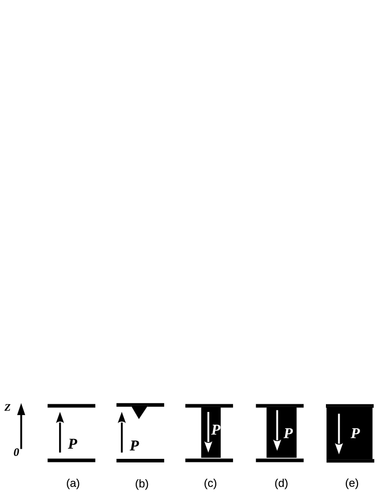
Figure 1: Simplistic switching process stages. (a) : homogeneous up-state , (b) : nucleation of a down-oriented region, (b) $\rightarrow$ (c): forward growth , (c) $\rightarrow$ (e): lateral growth , (e) homogeneous down-state.

Theoretically the direct switching mechanism as shown from (a) to (e) in Fig. 1 inside a delimited region [i.e. without considering the nucleation process (b)] can be described by using Landau approach in the presence of an electric field.

Due to the anisotropy, one can consider the switching mechanism induced by the electric field along the polarization axis $\mathbf{E}=E_{z}$ by using a one dimensional approach with the free energy functional $F=\int f\mathrm{d}V$ with $\mathbf{P}=P_{z}$ and

$$f(P_{z},E_{z})=\frac{\alpha}{2}P_{z}^{2}+\frac{\beta}{4}P_{z}^{4}+\frac{\kappa}{2}\left(\frac{\partial P_{z}}{\partial z}\right)^{2}-E_{z}P_{z}$$ (1)

In these conditions, the homegeneous switching mechanism with uniform $P_{z}$ uniform occurs by mean of progressive change in the polarization modulus and an abrupt change in sign when the field value reaches the thermodynamical coercive field $E_{c}=-\frac{2\alpha}{3\sqrt{3}}\sqrt{\frac{-\alpha}{\beta}}$ [Fig. 2(a)]. This field value is many orders of magnitude higher than the experimental coercive field , the difference between these two values being attributed to the crudeness of the nucleation process in the thermodynamical description, so that the switching mechanism is described as an homogeneous longitudinal phenomena (in reality ferroelectric switching always occurs via inhomogeneous nucleation). Some works have been devoted to extend this description to inhomogeneous switching by including the gradient energy and a surface term in the free energy BAUDRY_2005_2 ; BAUDRY_2007 , but nevertheless without solving the coercive field paradox.

Figure 2: Switching mechanisms : (a) longitudinal switching , (b) rotational switching .

Possible solution of this paradox can be in the shown in [Fig. 2(b)] switching of the polarization by means of a rotational homogeneous mechanism as it was proposed recently BAUDRY_2014 . In this case the polarization reversal occures without passing through the state $P=0$, but rather by rotation of its direction. Such mechanism we refer as ” Iwata switching” can be relevant for the cubic perovkite-type oxides in the bulk form, when the transition is described by the three-component order parameter $\mathbf{P}=(P_{x},P_{y},P_{z})$, and the free energy density $f$ has the following expression HU_1998 ; POTTER_2000 :

$$f(\mathbf{P},E_{z}) = \frac{\alpha}{2}\left(P_{x}^{2}+P_{y}^{2}+P_{z}^{2}\right)+\frac{\beta_{1}}{4}\left(P_{x}^{4}+P_{y}^{4}+P_{z}^{4}\right)+\frac{\beta_{2}}{2}\left(P_{x}^{2}P_{y}^{2}+P_{y}^{2}P_{z}^{2}+P_{z}^{2}P_{x}\right)+\frac{1}{2}G_{11}\left[(\partial_{x}P_{x})^{2}+(\partial_{y}P_{y})^{2}+(\partial_{z}P_{z})^{2}\right]$$ (2)

$$+G_{12}\left[\partial_{x}P_{x}\partial_{y}P_{y}+\partial_{y}P_{y}\partial_{z}P_{z}+\partial_{x}P_{x}\partial_{z}P_{z}\right]+\frac{1}{2}G_{44}[(\partial_{x}P_{y}+\partial_{y}P_{x})^{2}+(\partial_{z}P_{y}+\partial_{y}P_{z})^{2}+(\partial_{x}P_{z}+\partial_{z}P_{x})^{2}]+$$

$$\frac{1}{2}G_{44}^{\prime}[(\partial_{x}P_{y}-\partial_{y}P_{x})^{2}+(\partial_{z}P_{y}-\partial_{y}P_{z})^{2}+(\partial_{x}P_{z}-\partial_{z}P_{x})^{2}]-E_{z}P_{z}$$

However the potential problem of such scenario is the appearance of the surface bound charges provided by the perpendicular polarization component that is virtually emerged at the lateral sample during rotation. These charges produce the energy-unfavorable depolarization field that finally makes the homogeneous rotational switching inefficient in finite-size samples.

The proposed mechanism however can be realized via the non-uniform rotation of polarization vector inside the sample, when $\mathbf{P}$ stays parallel to the surface and bound charges do not appear at the boundary. In addition, the distribution of polarization inside the sample should satisfy the condition $\mathrm{div}\mathbf{P}=0$ to not cause the internal bound charges and related depolarization field.

In present article we investigate the possibility of such nonuniform switching, via the vortex formation mechanism as shown in [Fig. 2(b)]. To specify the geometry of the process we present the polarization vector in cylindrical coordinates $\mathbf{P}=(P_{\rho},P_{\varphi},P_{z})$ [Fig. 3].

Figure 3: Sketch of the structure studied.

From basic electrostatic considerations related to symmetry and invariance properties we have $P_{\rho}=0$, $P_{\varphi}(\rho)$ and $P_{z}(\rho)$. For the present case concerned with vortex formation, one can expect that it is also possible to switch the polarization by mean of progressive change in the angle $\theta$ ; we now investigate carefully such kind of possibility (i.e. switching by polarization rotation inside an ortho-radial plan with $\mathrm{div}\mathbf{P}=0$). In these conditions the free energy $f$ given by Eq. (2) becomes

$$f(\mathbf{P},E_{z}) = \frac{\alpha}{2}P_{\varphi}^{2}+\frac{\beta_{1}+\beta_{2}}{4}P_{\varphi}^{4}+\frac{\alpha}{2}P_{z}^{2}+\frac{\beta_{1}}{4}P_{z}^{4}+\frac{\beta_{2}}{2}P_{\varphi}^{2}P_{z}^{2}$$ (3)

$${}+G\left[\left(\frac{\partial P_{z}}{\partial\rho}\right)^{2}+\left(\frac{1}{\rho}\frac{\partial(\rho P_{\varphi})}{\partial\rho}\right)^{2}\right]-E_{z}P_{z},$$

where $G=G_{44}+G_{44}^{\prime}$.

Further simplification can be done close to the morphotropic phase boundary where the anisotropic terms in Eq. (3) are negligible and the rotational degrees of $\mathbf{P}$ are not coupled with its modulus. In this case we can use the constant modulus Goldstone approximation and parametrize the radial polarization distribution structure by the only parameter, which is the inclination angle $\theta(\rho)$. By introducing scalar variables $P$, $E$ related to the vectors components $P_{z}$, $P_{\varphi}$, $E_{z}$ by $P_{z}=P\cos\theta$, $P_{\varphi}=P\sin\theta$ and $E_{z}=-E$ (with $E>0$). We obtain the expression of the free energy with $\theta=\theta(\rho)$:

$$f(P,E) = \ GP^{2}\left[\left(\frac{\partial\theta}{\partial\rho}\right)^{2}+\frac{1}{\rho^{2}}\sin^{2}\theta+\frac{1}{\rho}\frac{\partial\sin^{2}\theta}{\partial\rho}\right]$$ (4)

$${}-PE\cos\theta.$$

It is convinient to use the rescaled quantities $\tilde{f}=\frac{f}{-\alpha_{0}\zeta_{0}^{2}P^{2}}$ and $\tilde{E}=\frac{E}{-\alpha_{0}\zeta_{0}^{2}P}$ where $\zeta_{0}=\sqrt{G/-\alpha_{0}}$ and $\alpha_{0}=\alpha\mid_{T=0}=-aT_{c}<0$. The parameter $\alpha=a(T-T_{c})$ being analogous to the coefficient of $P^{2}$ in the classical Landau free energy expansion (Eq. (1)).

Finally we obtain the expression of the rescaled free energy functional $\tilde{F}$ of the ferroelectric cylinder in the presence of the applied field

$$\tilde{F}=\int_{0}^{2\pi}\int_{0}^{R}\int_{0}^{h}\tilde{f}(\rho,\theta)\rho\mathrm{d}\rho\mathrm{d}\varphi\mathrm{d}z,$$ (5)

with

$$\tilde{f}(\rho,\theta)=\left(\frac{\partial\theta}{\partial\rho}\right)^{2}+\frac{1}{\rho^{2}}\sin^{2}\theta+\tilde{E}\cos\theta+\frac{1}{\rho}\frac{\partial\sin^{2}\theta}{\partial\rho}.$$ (6)

We are interested in a thin film homogeneously up-polarized at the initial state, i.e. with $\theta_{i}(\rho)=0$ , and would like to determine the possible final states obtained after applying a down electric field by mean of circular electrode with radius $R$. One can expect that there exist an intuitive solution which consists in a homogeneously down polarization state in the region where the field is applied (i.e. located under the circular electrode). In other words this solution for final state corresponds to $\theta_{f}(\rho)=\pi$ on the interval $[0,R]$. This solution is also from both mathematical and physical viewpoints a trivial solution when the diameter of the electrode is infinite, because it corresponds to a global minimum (polarization parallel to the field) for the free energy for an infinite system. For the case of real systems with finite electrode diameter, the finite character of the ferroelectric media would play an important role and the interaction with the exterior will be crucial via boundary conditions.

We have to solve a variational problem to search for functions $\theta(\rho)$ which are extrema of the functional $\tilde{F}$ and first develop the variation of the functional by carefully paying attention to the contribution of boundary conditions.

$$\delta\tilde{F} = 2\pi h\int_{0}^{R}g(\theta(\rho,e))\delta\theta\mathrm{d}\rho+2\pi h\left[\frac{\partial\theta}{\partial\rho}\delta\theta\right]_{0}^{R}$$ (7)

$$+2\pi h\left[\frac{1}{2}\sin 2\theta\delta\theta\right]_{0}^{R},$$

with

$$g(\theta(\rho,e))=-2\nabla_{\rho}^{2}\theta+\frac{1}{\rho^{2}}\sin 2\theta-e\sin\theta.$$ (8)

In order to find non trivial solutions we have assumed that the polarization was pinned in the initial up-oriented polarization state $\rho=0$ and $\rho=R$, so that the value of $\theta(0)=0$ and $\theta(R)=0$ are fixed and independed on the field.

Finally variational calculation leads to the following state equation expressed in terms of rescaled variables $\tilde{\rho}=\rho/R$ and $\tilde{e}=\tilde{E}R^{2}\geq 0$ :

$$\frac{\partial^{2}\theta}{\partial\tilde{\rho}^{2}}+{\frac{1}{\tilde{\rho}}}\frac{\partial\theta}{\partial\tilde{\rho}}-\frac{1}{2\tilde{\rho}^{2}}\sin 2\theta+\frac{\tilde{e}}{2}\sin\theta=0.$$ (9)

The determination of the extremum of the functional requires one to solve the previous nonlinear second order differential equation with corresponding boundary conditions for $\theta(\tilde{\rho},\tilde{e})$ at $\tilde{\rho}=0$ and $\tilde{\rho}=1$.

We obtain the equilibrium state by using a numerical method suitable for solving the nonlinear state equation Eq. 9. We have plotted in Fig. 4 the evolution of the maximum $\theta_{\mathrm{max}}=\max\theta(\tilde{r})$, as function of rescaled electric field $\tilde{e}/\tilde{e_{0}}$ with $\tilde{e}=\tilde{e}_{0}\approx 29.36$. There exist a critical field $\tilde{e}_{c-\mathrm{min}}^{\star}\approx 0.94\tilde{e}_{0}$ upon which there exist non zero solutions of Eq. (9). Between $\tilde{e}_{c-\mathrm{min}}^{\star}$ and $\tilde{e}_{c-\mathrm{max}}^{\star}=\tilde{e}_{0}$ there are two possibilities for vortex state with two different values for $\theta_{\mathrm{max}}$. From $\tilde{e}_{c-\mathrm{min}}^{\star}$ we observe two branches, the first one with negative slope reaches $0$ at $\tilde{e}_{c-\mathrm{max}}^{\star}$ and the second one with positive slope which approaches $\tilde{e}_{c-\mathrm{max}}^{\star}$. In order to determine the state which is the most stable we have plotted in Fig. 5 the evolution of the free energy $\tilde{F}$ as a function of $\tilde{e}/\tilde{e_{0}}$ from the different kinds of solutions. With the dotted line, we have represented the free energy $\pi h\tilde{e}$ of the homogeneous up-oriented state. From $\tilde{e}_{c-\mathrm{min}}^{\star}$ we observe also the evolution of the free energy which corresponds to the two branches previously described in Fig. 4. The curve with dashed line in Fig. 5 corresponds to the part of the curve with dashed line in Fig. 4. In that case the energy is greater than the energy $\pi h\tilde{e}$ of the trivial solution $\theta=0$ all over the range of fields $\tilde{e}_{c-\mathrm{min}}^{\star}-\tilde{e}_{c-\mathrm{max}}^{\star}$ for which this solution exists, so that it doesn’t corresponds to the more stable state which remains the homogeneous up state. The curve with solid line in Fig. 5 corresponds to the part of the curve with solid line in Fig. 4 also exhibit an energy greater than $\pi h\tilde{e}$ up to $\tilde{e}=\tilde{e}_{c-\mathrm{abs}}^{\star}\approx 0.96\tilde{e}_{0}$ so that the vortex state less stable than the homogeneous state. On the contrary, upon reaching $\tilde{e}=\tilde{e}_{c-\mathrm{abs}}^{\star}$ the energy of the second solution, is lower than $\pi h\tilde{e}$. As a consequence this second solution corresponds to the more stable solution in the presence of an applied field greater than $\tilde{e}_{c-\mathrm{abs}}^{\star}$. At $\tilde{e}=\tilde{e}_{c-\mathrm{max}}^{\star}$ we observe the existence of a single solution which corresponds to the prolongation of the second solution in the range $\tilde{e}_{c-\mathrm{min}}^{\star}-\tilde{e}_{c-\mathrm{max}}^{\star}$ [Fig. 5]. We have represented in Fig. 6 the distribution $\theta(\tilde{r})$ for different electric fields. The shape observed for the metastable state at $\tilde{e}_{c-\mathrm{min}}^{\star}$ is slighly asymmetric. It becomes more asymmetric as $\tilde{e}$ increases. For the highest electric field the $\theta(\tilde{r})$ distribution is highly asymmetric which reveals an important characteristic of the vortex state.

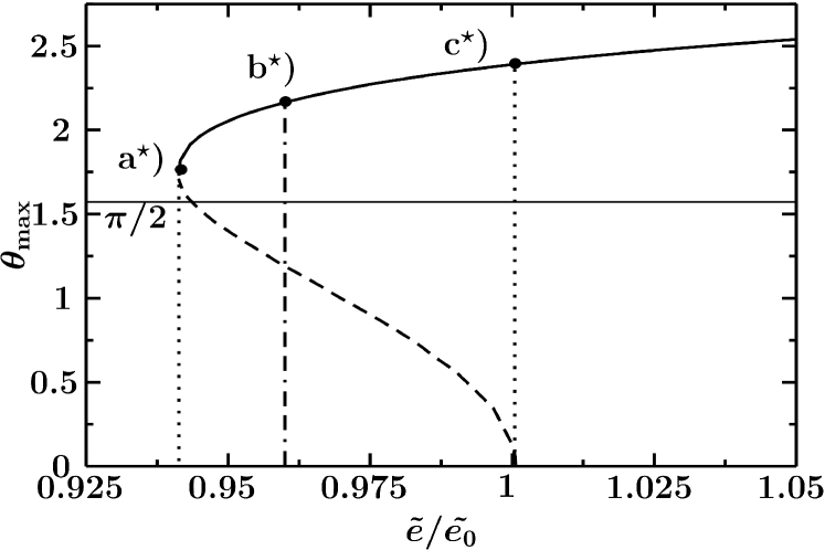
Figure 4: Maximun value of $\theta(\tilde{\rho})$ as a function of $\tilde{e}/\tilde{e}_{0}$. The solid and dashes line respectively corresponds to two differents vortex states with different free energy minimum $\tilde{F}$ (Fig. 5). Particular selected points correspond to : a^⋆) $\tilde{e}_{c-\mathrm{min}}\approx 0.94\tilde{e}_{0}$, b^⋆) $\tilde{e}_{c-\mathrm{abs}}\approx 0.96\tilde{e}_{0}$and c^⋆) $\tilde{e}_{c-\mathrm{max}}=\tilde{e}_{0}$. Vertical dashed-dotted lines correspond to critical fields for transition between absolute stable states. The range of field values delimited by vertical dotted line corresponds to the maximal extension of possible electric hysteresis phenomena.

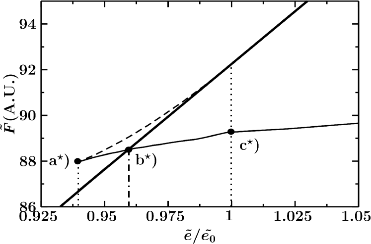
Figure 5: Energy $\tilde{F}$ as a function of $\tilde{e}/\tilde{e}_{0}$ for different polarization distribution : homogeneous up-state (thick solid line), vortex state $\mathrm{d}\theta_{\mathrm{max}}/\mathrm{d}\tilde{e}<0$ (dashed line) and vortex state $\mathrm{d}\theta_{\mathrm{max}}/\mathrm{d}\tilde{e}>0$ (solid line). Particular selected points correspond to : a^⋆) $\tilde{e}_{c-\mathrm{min}}\approx 0.94\tilde{e}_{0}$, b^⋆) $\tilde{e}_{c-\mathrm{abs}}\approx 0.96\tilde{e}_{0}$and c^⋆) $\tilde{e}_{c-\mathrm{max}}=\tilde{e}_{0}$.

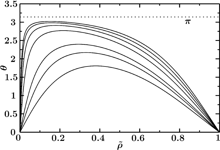
Figure 6: $\theta$ as a function of $\tilde{\rho}$ for different electric field values, from the bottom to the top: a^⋆) $\tilde{e}_{c-\mathrm{min}}\approx 0.94\tilde{e}_{0}$ , b^⋆) $\tilde{e}_{c-\mathrm{abs}}\approx 0.96\tilde{e}_{0}$, c^⋆) $\tilde{e}_{c-\mathrm{max}}=\tilde{e}_{0}$, $1.2\tilde{e}_{0}$, $1.4\tilde{e}_{0}$, $1.6\tilde{e}_{0}$, $1.8\tilde{e}_{0}$.

III DISCUSSION OF EXPERIMENTAL SITUATIONS

The experimental study of circular closure or vortex domains began experimentally with the study by Dawber et al. DAWBER_2003 of nucleation and growth of ferroelectric domains in unpoled PZT films. By measuring the frequency response of thin films to ac signals, they found that a resonance was observed with frequency equal to the reciprocal of the specimens perimeter. This relationship was interpreted as nucleation at the edge, propagation around the circumference, leaving an unswitched core at the center. The effect was not proportional to the diameter or area of the specimen, only perimeter, as verified by using square and rectangular samples of very different aspect ratios, from 1 $\times$ 1 $\mu$m to 130 $\times$ 180 $\mu$m (4 $\mu$m to 620 $\mu$m). However, these circular closure domains were not initially tested via direct spatial observation, either electron microscopy, optical microscopy, or PFM. It is important in the present context that these closure domains were observed only in films that had not been pre-poled but which had simply been cooled from above the Curie temperature. Even more important, this was observed to be a low-field phenomenon. It occurred only for $E<<100\mathrm{kV/cm}$ and in fact could occur for fields $\times$10 smaller than the nominal coercive field $E_{c}$. For larger applied fields, the switched polarization was homogeneous, from $+P$ to $-P$, with no unswitched hole in the center. This early work implied two distinct coercive fields : a low coercive field for vortex instability, and a higher coercive field for homogeneous switching. However, these experiments showed that the speed of propagation of the closure domain was given ballistically STEVENSON_1966 by the formula

$$\tau=\frac{2\lambda}{v_{0}}\exp\left(\frac{R}{2l}\right),$$ (10)

where $R$ is the disc radius, $l$ is the phonon wavelength causing viscuous drag with coefficient and $v_{0}$ the domain wall velocity.

$$D=\frac{1}{2}\rho Av_{0}^{2},$$ (11)

$\rho$ is the sample density and $A$ is the cross section. Velocity $v_{0}$ was fitted to be $3\mathrm{m/s}$ in PZT. In the present model we not only assume a much faster wall velocity, but we neglect damping.

The second experimental paper GRUVERMAN_2008 revealed spatially (via PFM) and with 100 ns time resolution, closure domains in circular discs at higher fields (ca. $70\mathrm{kV/cm}$) but not in squares of the same diameter (2 $\mu$m) and thickness, indicating a significant role of boundary conditions. A model simulation, based upon ferromagnetic Landau-Lifshitz-Gilbert equations reproduced the experiments well and also indicated that this is a low-field phenomenon. Further modeling by the authors of Ref. GRUVERMAN_2008 showed that there was a critical size for these closure domains, which for discs was ca. 2-micron diameter and smaller for squares. Triangular specimens in the simulation did not exhibit closure domains for any field or lateral size.

The third experimental paperSCOTT_2008 showed that the circular unswitched center[Fig. 7] in the closure domains was only metastable and disappeared in zero field after ca. 24 hours. At longer times the outer edge became faceted along high-symmetry planes, indicating relaxation caused by crystalline anisotropyGANPULE_2002 ; LUKYANCHUK_2014

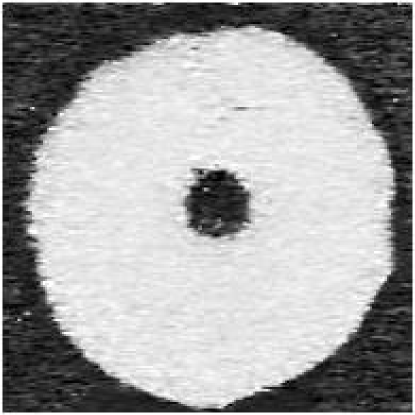
Figure 7: Closure domain with circular unswitched center (adapted from Ref. GRUVERMAN_2008 )

Most recently the study of closure domains in nano-dotsSCHILLING_2009 revealed that they arise from experimentally cooling through $T_{c}$ with very small or zero field. This time simulation was done via a standard finite element micromagnetics software MAGPAR SCHOLZ_2003 and again supported the experiments. The MAGPAR calculation had been done as a simple magnetic domain analogy and surprisingly displays the basic qualitative features of the experiment, although unlike the present work it offers no explanation for the real mechanism or numertical values. It does illustrate the sensitivity to boundary conditions and size in the problem, and the basic Bessel-function-like solutions.

Taken as a whole, these experiments show, in agreement with the theory above, that there are two coercive fields in ferroelectric nano-dots: A very small coercive field for vortex instability switching $E^{\mathrm{vortex}}_{c}$; and a large coercive field for conventional switching $E_{c}$ from homogeneous $+P$ to $-P$ states. There is an indication that there may be a critical radius for these effects, but that is uncertain; none was found in Ref.DAWBER_2003 .

These closure domains may have important application for memory storage in ferroelectric memories (FRAMs): as Prosandeev et al. have shown,PROSANDEEV_2007 ; PROSANDEEV_2008 these configurations permit very high bit-density and can be reversed by application of external electric fields.

IV DYNAMICAL PROPERTIES

Up to now we have studied the static case and determined the equilibrium polarization state in the presence of an electric field. We now turn our attention to discuss the essence of the dynamical polarization reversal process on the basis of the Landau-Khalatnikov equation of motion. The evolution of the polarization with time is expressed as follow :

$$\frac{\partial P_{i}}{\partial t}=-L_{i}\frac{\delta F}{\delta P_{i}},$$ (12)

where $L_{i}$ are the damping coefficients, $i$ =$\left\{\varphi,z\right\}$.

In our model the time evolution of the polarization is parametrized by the inclination angle $\theta$ and corresponding Landau-Khalatnikov looks like

$$\frac{\partial\theta}{\partial t}=-L\frac{\delta F}{\delta\theta}.$$ (13)

The switching mechanism is initiated by a weak angle instability $\delta\theta$. For a field $e>\tilde{e}_{c}$ we observe the polarization switching by mean of progressive change of the angle $\theta$. This phenomena is inhomogeneous and first affects a region located close to the half-radius of the electrode. Then we distinguish two stages, the first one which is almost symmetric with respect to the half-radius and a second one which consists in a radial extension of the switched region.

We present in Figs. 8(a) and  8(b) the time evolution of the polarization profile during the switching process. On the whole this polarization reversal exhibits characteristics similar to the process in thin films described in Fig. 1 : the switching occurs in the orthoradial direction and is followed by a growth in a perpendicular radial direction. This suggests that behavior of polarization component could be an universal characteristic of the switching mechanism in ferroelectric materials.

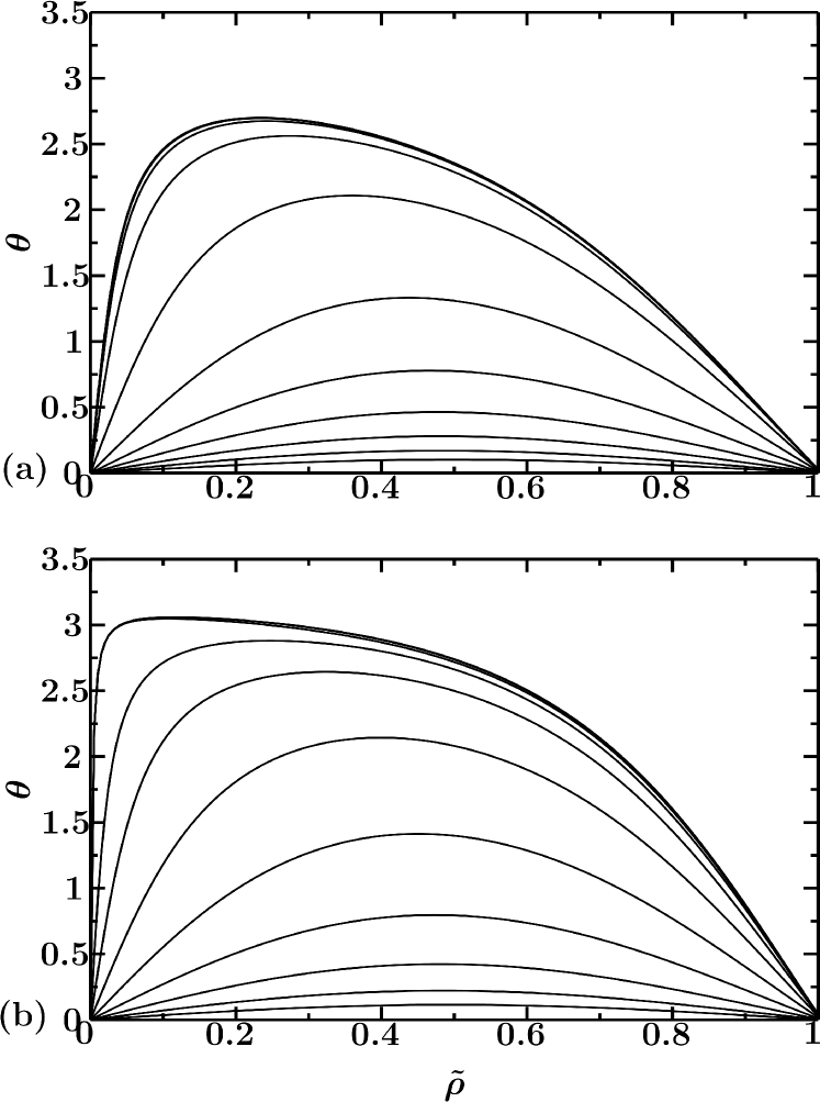
Figure 8: From the bottom to the top : evolution of the distribution $\theta(\tilde{\rho})$ with time for $\tilde{e}=1.2\tilde{e}^{\star}_{c-\mathrm{min}}$ (a) and $\tilde{e}=2\tilde{e}^{\star}_{c-\mathrm{min}}$ (b). At the initial time the polarization is homogeneous and up oriented $(\theta=0)$. The time-step values and the value of $L$ are chosen to favor the visualization of the evolution of $\theta(\tilde{\rho})$ until the final state is reached (curve at the top of the figure).

In order to test the capability of our model to describe the experimental behavior, we have carefully examined the results reported by GruvermanGRUVERMAN_2008 , and compared with those given by our model by mean of quasi-2D numerical simulation. Main characteristics of PFM measurements are : i) nucleation of down state at different places, ii) orthoradial rotation, iii) radial rotation which leads to doughnut with small central peripheral unswitched region. Our simulation considers that there exist latent nuclei which corresponds to regions with instabilities $\delta\theta$, at different places that are sample-dependent and adopted Gruverman’s data. Fig. 9 shows the two-dimensional angular distribution of $\theta(\tilde{\rho},\varphi)$. The initial state and a stage which corresponds to the appearance of many switched regions are respectively reproduced in Fig. 9(a) and (b). The next stages reproduce orthoradial extension [Fig. 9(c) and (d)] which can be interpreted as a time delay between polarization rotation induced by the inhomogeneous nature of the instabilities distribution $\delta\theta(\tilde{\rho},\varphi)$. It leads to doughnut shape with large central unswitched region. The last stage corresponds the radial rotation which contributes to reduction of the central region area [Fig. 9(e)]. At the end of the process when the stable state is reached [Fig. 9(f)], the doughnut shape reported by Gruverman, with small central region and peripheral unswitched region is obtained.

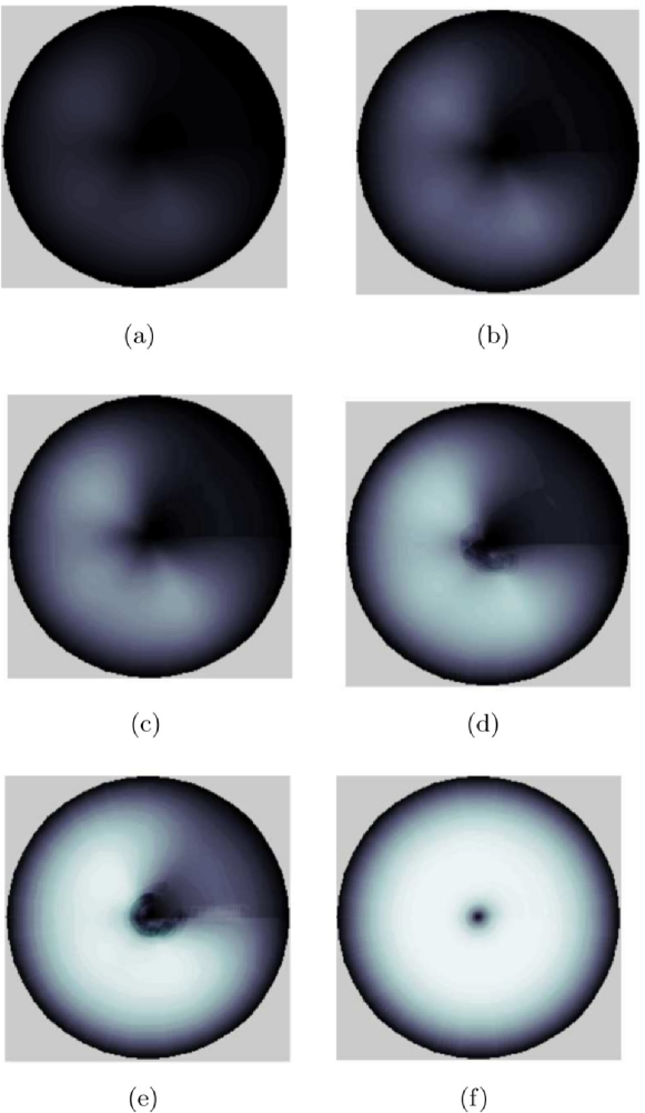
Figure 9: Evolution of the polarization texture below the circular electrode during the switching process. With black color : the ”up” state, with white color the ”down” state.

V CONCLUSION

We have considered a finite ferroelectric cylinder with top and bottom electrodes used to apply an electric field. By using a thermodynamical approach we have demonstrated that there exist non-trivial mathematical solutions induced by the boundary conditions at the perimeter of the cylinder. These solutions correspond to a metastable polarization state and are observed only when an external electric field is greater than a coercive value $\tilde{e}_{\mathrm{coercive}}$. We have also demonstrated that the switching mechanism have the behaviour of a field-induced discontinous transition with hysteresis in the interval $\tilde{e}_{c-\mathrm{min}}^{\star}-\tilde{e}_{c-\mathrm{max}}^{\star}$. However, the kinetic contribution can influence the precise value of coercive field $\tilde{e}_{\mathrm{coercive}}$, which would not strongly deviate from the range $\tilde{e}_{c-\mathrm{min}}^{\star}-\tilde{e}_{c-\mathrm{max}}^{\star}$. One can argue that the order of magnitude of $\tilde{e}_{\mathrm{coercive}}$ is given by the value $\tilde{e}_{0}$ itself and is governed by the boundary condition at the perimeter of the electrode. One can estimate the coercive field for the vortex-formationg switching by the field $E_{\mathrm{c}}^{\mathrm{vortex}}=\alpha_{0}\left(\frac{\zeta_{0}}{R}\right)^{2}P\tilde{e}_{0}$ and compare it with the classical thermodynamic coercive field $E_{\mathrm{c}}$. These two fields are found to be equal when $R=R_{0}\approx 8.73\zeta_{0}$. Usually $R>R_{0}$ and $E_{\mathrm{c}}^{\mathrm{vortex}}<E_{\mathrm{c}}$.

In the case of Gruverman’s GRUVERMAN_2008 study, one can estimate from the experimental parameters the value of $E_{\mathrm{c}}^{\mathrm{vortex}}$. It is found to be many times lower than the rectilinear-domain coercive field. In these conditions it seems reasonable that the existence of a coercive field for vortex formation has not been reported in Gruverman’s GRUVERMAN_2008 article. The evolution of the polarization texture in two-dimensional films allowed us to describe the vortex formation. The calculated final steady state is similar the unusual domain pattern with doughnut shape previously experimentally observed only in the case of circular capacitor GRUVERMAN_2008 . The metastable characteristic of the doughnut distribution SCOTT_2008 is also followed from our consideration since it vanishes when the electric field is suppressed. The fact that the central and peripheral unswitched regions are very small is also consistent with the results given by the present theory which predicts polarization saturation with $\theta=\pi$ along the radius and unswitched regions with $\theta=0$ at the center and at the peripheral edge of the electrode. The effect of the electric field tends to enlarge the proportion of the region where the polarization saturates and to decrease the central and the peripheral regions. The dimensions of the unswitched regions are very small, which is revelant for an applied electric field much higher that the value given by our calculation. Hence one should carefully investigate experimentally the role of the applied field on the possible vortex formation. Since the polarization reversal rotationnal mechanism costs less energy than the classical one provided by change in the modulus, usually observed in thin films, one can expect that this alternative switching mechanism, induced by both the geometry and the interface properties would be especially useful in memory-storage.

- (1) M. Dawber, K. M. Rabe, and J. F. Scott, Rev. Mod. Phys. 77, 1083 (2005).
- (2) D. Tilley and B. Zeks, Solid State Commun. 49, 823 (1984).
- (3) D. Tilley and B. Zeks, Ferroelectrics 134, 313 (1992).
- (4) F. De Guerville, I. Luk’yanchuk, L. Lahoche, and M. El Marssi, Material science engeneering B 120, 16 (2005).
- (5) I. A. Luk’yanchuk, L. Lahoche, and A. Sene, Phys. Rev. Lett. 102, 147601 (2009).
- (6) C.-L. Jia, K. W. Urban, M. Alexe, D. Hesse, and I. Vrejoiu, Science 331, 1420 (2011).
- (7) N. Balke et al., Nat. Phys. 8, 81 (2012).
- (8) A. Gruverman et al., J. Phys. : Condens. Matter 20, 342201 (5pp) (2008).
- (9) J. F. Scott, A. Gruverman, D. Wu, I. Vrejoiu, and M. Alexe, J. Phys. : Condens. Matter 20, 425222 (5pp) (2008).
- (10) Discrepancy known as coercive field paradox.
- (11) L. Baudry, Appl. Phys. Lett. 87, 262903 (2005).
- (12) L. Baudry, Int. Ferroelectrics 91, 10 (2007).
- (13) L. Baudry, I. A. Lukyanchuk, and A. Razumnaya, arXiv:1403.4191 .
- (14) H.-L. Hu and L.-Q. Chen, J. Am. Ceram. Soc. 81, 492 (1998).
- (15) J. B. G. Potter, V. Tikare, and B. A. Tuttle, J. Appl. Phys. 87, 4415 (2000).
- (16) M. Dawber, D. J. Jung, and J. F. Scott, Appl. Phys. Lett. 82 (2003).
- (17) R. W. H. Stevenson, Phonons in perfect lattices and in lattices with point imperfections, page p 255, Oliver & Boyd Scottish Universities Summer School in Physics (06 ; 1965 ; Aberdeen, Scotland), Edinburgh London, 1966.
- (18) C. S. Ganpule et al., Phys. Rev. B 65, 014101 (2001).
- (19) I. A. Lukyanchuk et al., arXiv:1309.0291 .
- (20) A. Schilling et al., Nano Letters 9, 3359 (2009).
- (21) Computational Materials Science 28, 366 (2003).
- (22) S. Prosandeev and L. Bellaiche, Phys. Rev. B 75, 094102 (2007).
- (23) S. Prosandeev, I. Ponomareva, I. Kornev, and L. Bellaiche, Phys. Rev. Lett. 100, 047201 (2008).