Abstract

Abstract

The Large Hadron Collider (LHC) is the first machine that provides high enough energy to produce large numbers of boosted top quarks. The decay products of these top quarks are confined to a cone in the top quark flight direction and can be clustered to a single jet. Top quark reconstruction then amounts to analysing the structure of the jet and looking for subjets that are kinematically compatible with top quark decay. Many techniques have been developed recently to best use these topologies to identify top quarks in a large background of non-top jets. This article reviews the results obtained using LHC data recorded in the years 2010–2012 by the experiments ATLAS and CMS. Studies of Standard Model top quark production and searches for new massive particles that decay to top quarks are presented.

1 Introduction

The Large Hadron Collider (LHC) at the European particle physics research centre CERN in Geneva, Switzerland, is a discovery machine at the energy frontier. A primary goal, the observation of the Higgs boson, has already been achieved [1, 2]. Other important research topics are searches for deviations from predictions of the Standard Model of particle physics (SM). This review is concerned with processes that involve the heaviest known elementary particle, the top quark. Due to its mass it is expected to play an important role in electroweak symmetry breaking.

The top quark is reconstructed via its decay products which are collimated if the top quark Lorentz factor $\gamma=E/m$ is large. The top quark is then boosted and the decay products are confined to a cone with an opening angle that depends inversely on $\gamma$. All particles inside the cone can be clustered into a jet, the structure of which reflects the top quark decay pattern. The first paper on this topic was published in 1994 by Seymour [3].

The LHC is the first machine that provides high enough energy to produce large numbers of boosted top quarks. The study of boosted topologies has seen an explosion of interest after it had been shown in 2008 by Butterworth et al. [4] that the boosted signature makes possible the use of hadronic decay channels in searches at the LHC. These channels have often the highest branching ratio but had been deemed infeasible before because of the large background at a hadron-hadron machine. In the years following, many aspects of jet structure have been investigated in the light of the identification of boosted top quarks and boosted $W$, $Z$, and Higgs bosons. The crucial point has always been how well the jets that include the decay products of a heavy particle can be distinguished from background jets that originate from hard light quarks or gluons, so-called QCD jets (events in which the jet activity is given solely by QCD jets are referred to as multijet events).

After the start of the LHC, the two multipurpose experiments ATLAS and CMS began studying the behaviour of jet structure techniques in the real world. Before these techniques could be used in analyses, a number of basic and technical works had to be carried out, some of which are listed in the following. The jets in top quark reconstruction are much larger than the ones used to reconstruct the kinematics of single partons. These large jets, so-called fat jets, first need to be calibrated. Then the precision with which simulations can model the jet structure observed in the detector had to be quantified so that comparisons with predictions became meaningful. The quality of predictions of the parton shower and hadronisation needed to be assessed which is especially important in the context of large jets that contain several hard partons, some of which may be connected by colour strings. In addition, the situation is complicated by the presence of overlay signals that result from slow detector read-out and additional particles due to multiple inelastic proton-proton ($pp$) interactions. The size of the large jets makes them especially susceptible to this so-called pile-up energy.

The techniques have been studied using SM processes in $pp$ collisions at centre-of-mass energies $\sqrt{s}=7$ and $8{\mathrm{\ Te\kern-1.00006ptV}}$. Background samples that are dominated by jets which do not contain top quark decay products are easily obtained and the jet structure was studied extensively. Samples of events with a top quark and an anti-top quark ($t\bar{t}$ pair) were obtained through a conventional selection, i.e., without applying jet structure techniques. These events were used to test the performance of boosted top quark reconstruction methods and to evaluate systematic uncertainties. This made first applications of jet structure techniques in physics analyses possible. These were searches for new TeV-scale particles that decay to highly energetic top quarks. To this day, these types of searches feature prominently in the analysis of ATLAS and CMS data.

After the repair of the LHC, in collisions at $\sqrt{s}=13{\mathrm{\ Te\kern-1.00006ptV}}$ in 2015, the cross sections of other important processes will be high enough to allow the application of jet structure techniques. One example is the associated production of a Higgs boson with a $t\bar{t}$ pair [5]. The measurement of the production cross section of this process will allow the extraction of the coupling strength between the Higgs boson and the top quark. This is the largest Higgs coupling in the SM and deviations from the SM prediction would indicate New Physics.

Jet structure and its application to identify bosons and top quarks is a new and extremely rich field, both on the phenomenological and on the experimental side. Many questions need to be addressed and new developments are emerging from the collaboration of theorists and experimentalists. The most important annual meeting of the community is the BOOST workshop, of which reports are published in [6, 7]. A theoretical review of jet structure methods is given in [8]. For a review of mostly conventional LHC top quark analyses see [9].

This article reviews the current state of boosted top quark reconstruction using jet structure techniques and its application in physics analyses. For future searches, a new method is presented that overcomes current experimental limitations in the regime of very high top quark energies. The review closes with an outlook on the future of the field.

2 Motivation

This section introduces the basic ideas behind jet structure methods and how they can be used to find top quarks. With the currently available data, the strongest impact of these techniques is in searches for physics beyond the SM. Two New Physics models are described that have been used in the analyses discussed in Section 10.

2.1 Top quark production and decay

The top quark is the heaviest particle in the SM. The current Particle Data Group top quark mass is $173.07\pm 0.52({\rm stat.})\pm 0.72({\rm syst.}){\mathrm{\ Ge\kern-1.00006ptV}}$ [10, 11], obtained from measurements at the Tevatron. The probability to produce top quarks in particle collisions is small because of the large mass. Predictions for (total) SM production cross sections in $pp$ and $p\bar{p}$ collisions are shown in Figure 1 and ATLAS measurements of SM production processes are summarised in Figure 2. The cross sections are dominated by soft collisions in which little energy is exchanged and the outgoing particles do not acquire large momenta transverse to the beam line. The total inelastic $pp$ cross section at $\sqrt{s}=7{\mathrm{\ Te\kern-1.00006ptV}}$ was measured to be $70(7)$ mb [12]. At this energy, hard parton scattering, leading to jets with transverse momentum ($p_{\rm T}$) larger than $100{\mathrm{\ Ge\kern-1.00006ptV}}$, has a cross section of $\approx 4\times 10^{5}$ pb, approximately five orders of magnitude smaller. The $W$ boson production cross section is $\approx 10^{5}$ pb. The pair-production cross section for top quarks at approximate next-to-next-to-leading order (NNLO) in QCD is $167$ pb when using the MSTW2008 NNLO proton parton densities [13] and the HATHOR Monte Carlo program [14]. This is approximately a factor $1/2000$ smaller than the jet cross section. This illustrates that top quark physics at the LHC has to fight large backgrounds from jets and/or $W$ boson production.

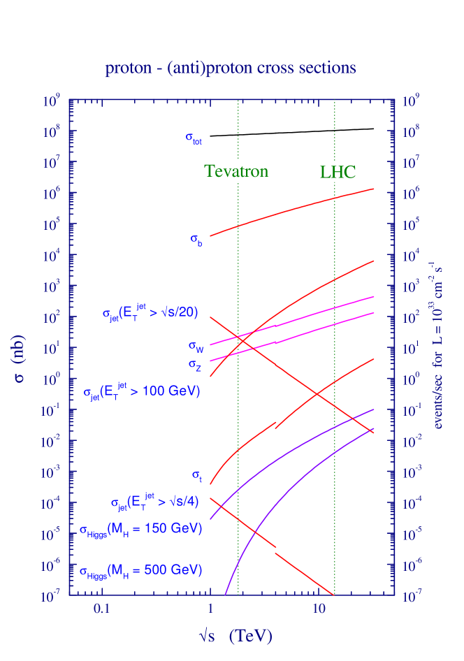
Figure 1: Predictions for proton-(anti-)proton SM production cross sections as a function of the centre-of-mass energy $\sqrt{s}$. The Tevatron energy ($1.96{\mathrm{\ Te\kern-1.00006ptV}}$) and the design energy of the LHC ($14{\mathrm{\ Te\kern-1.00006ptV}}$) are indicated. From [15].

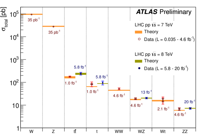
Figure 2: Measurements of several SM production cross sections. Also shown are theory predictions. From [16].

The top quark decay width predicted by the SM at next-to-leading order (NLO) is $\approx\!1.3{\mathrm{\ Ge\kern-1.00006ptV}}$, corresponding to a lifetime of $\approx\!0.5\times 10^{-24}\,$s [17]. The CKM matrix element $V_{tb}$ is estimated to be larger than 0.999, indicating that almost all top quarks decay according to $t\rightarrow Wb$. The $W$ boson decays in $67\%$ of the cases to two quarks (hadronic decay), the branching ratio to a neutrino and a lepton is $11\%$ for each lepton flavour. The tau lepton decays in $34\%$ of the cases to an electron or a muon and these cases look experimentally like direct $W$ boson decays to electron or muon. The electron and muon channels (including the corresponding $\tau$ decays) are collectively referred to as leptonic decay.

For decays of pairs of top quarks ($t\bar{t}$) the decays are to $45\%$ hadronic (both top quarks decay hadronically) and to $35\%$ semileptonic ($e/\mu$+jets, one top quark decays leptonically). The rest of the decays are dileptonic decays and hadronic tau decays.

2.2 Boosted particle decays

The LHC can produce particles with kinetic energies much larger than the electroweak scale. In the laboratory frame, the decay products of such a particle are collimated in the particle flight direction. This poses new experimental challenges compared to decays at rest. The difference between decay at rest and boosted decay is illustrated in Figure 3. A particle $X$ decays to two jets. If $X$ is at rest, the two jets are well separated and will be detected as two distinct jets. If $X$ is boosted, the two jets are collimated in the forward direction. If the boost of $X$ is large enough, the two jets merge into a large single jet (fat jet). The structure of this fat jet contains information about the decay.

Figure 3: Schematic diagrams of the decay of a particle $X$ to two jets when the particle is at rest (left) and boosted (right). In the boosted case, the two jets merge into a single fat jet. The fraction of the particle momentum taken by one of the jets is denoted by $z$. From [18].

For a two-body decay, the distance of the decay products in rapidity-azimuth space $(y,\phi)$ is given by

$$\Delta R\approx 2m/p_{\rm T}$$ (1)

in which $m$ and $p_{\rm T}$ are the mass and transverse momentum of the decaying particle, respectively. For a $W$ boson with $p_{\rm T}=200{\mathrm{\ Ge\kern-1.00006ptV}}$, the distance is $\Delta R=0.8$ and $\Delta R=0.5$ for $p_{\rm T}=320{\mathrm{\ Ge\kern-1.00006ptV}}$. The conventional jets used in the LHC experiments cover distances $\Delta R=0.4$–$0.6$. With these jets, the two decay products of a highly energetic $W$ boson cannot be resolved and conventional reconstruction techniques fail. The same is true for the decays of other boosted particles, like $Z$ bosons, Higgs bosons, and top quarks.

The minimal size of a $\mathrm{C/A}$ jet that contains the decay quarks in hadronic top quark decay, $t\to bqq$, is shown in Figure 4 as a function of the top quark $p_{\rm T}$. This size corresponds to the minimal radius parameter $R$ that would have to be used in a jet to capture the three quarks (cf. Section 3.1). Even jets with $R=1.5$ catch only a small fraction of top quark decays with $p_{\rm T}=200{\mathrm{\ Ge\kern-1.00006ptV}}$.

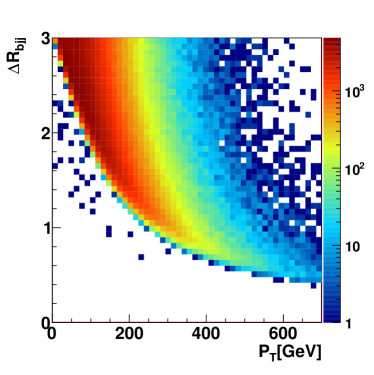
Figure 4: The minimal size of a $\mathrm{C/A}$ jet that contains the decay quarks in the decay $t\rightarrow bqq$ as a function of the top quark $p_{\rm T}$. From [19].

Conventional techniques that rely on the detection of isolated decay products fail when those products are collimated and merged into single reconstructed objects, such as jets. It is the analysis of the internal structure of these objects that offers a way to identify and measure boosted particles.

Figure 5: Normalised transverse momentum distributions in simulated LHC events at $\sqrt{s}=14{\mathrm{\ Te\kern-1.00006ptV}}$ for associated $t\bar{t}$ pair plus Higgs boson production (ttH) and background processes ($W\!$+jets production, Wjj, and W+H production). Shown are the $p_{\rm T}$ distributions of the top quarks ($p_{{\rm T,t}}$), the Higgs boson ($p_{{\rm T,H}}$) and the leading $p_{\rm T}$ jet ($p_{{\rm T,j}}$) as predicted by MadGraph+HERWIG++. From [5].

Boosted techniques are also useful if the background falls more rapidly with $p_{\rm T}$ than the signal. An example of this kind is the analysis of associated Higgs boson production with a $t\bar{t}$ pair [5]. Shown in Figure 5 are the $p_{\rm T}$ spectra of the involved particles: the distributions for the Higgs boson and the top quarks are harder than those for the background. An analysis in the boosted regime can therefore have the advantage of an enhanced signal-to-background ratio (S/B).

2.3 Higgs mass fine-tuning

Boosted particles are also frequently encountered in extensions of the SM. In these theories and models, new heavy particles are proposed with masses at or above the TeV scale. The SM particles to which these new states decay are highly boosted, making jet structure techniques ideal discovery tools. The new theories are introduced to overcome shortcomings of the SM, such as the hierarchy problem and the Higgs mass fine-tuning.

In the SM, electroweak symmetry breaking (EWSB) occurs due to the introduction of a scalar weak isospin Higgs doublet. One component of the doublet has a non-vanishing vacuum expectation value (VEV). Upon expanding the complex doublet Higgs field in four real fields about the VEV, three of the fields are massless (the Nambu-Goldstone bosons, NGB) and one field gains mass (the Higgs boson). In the unitary gauge, the three NBGs are eaten by the vector bosons $W^{+},W^{-},Z$ and give them mass.

One of the puzzles of the SM is the fine-tuning of the radiative corrections to the Higgs mass. These large corrections appear because the Higgs boson is a scalar. By contrast, fermion masses are protected by a custodial symmetry as follows [20]. The fermion spinors can be decomposed into left- and right-handed components (using the projection operators $P_{R,L}=(1\pm\gamma^{5})/2$). In the massless limit, the free Lagrangian decomposes into two terms, one for each chiral component:

$$\mathscr{L}=\overline{\psi}i\mbox{$/{\!\!\!\partial}$}\psi=\overline{\psi_{L}}i\mbox{$/{\!\!\!\partial}$}\psi_{L}+\overline{\psi_{R}}i\mbox{$/{\!\!\!\partial}$}\psi_{R}\,.$$ (2)

This Lagrangian is invariant under two independent global symmetry transformations. For example, for the massless electron in QED, the symmetries are $U(1)_{L}$ and $U(1)_{R}$, which act only on the left- and right-handed components, respectively. The theory is chiral because it distinguishes between left and right handedness and $U(1)_{L}\times U(1)_{R}$ is called chiral symmetry. An explicit mass term $-m\overline{\psi}\psi$ would couple both chiralities and break $U(1)_{L}\times U(1)_{R}$. It turns out that the chiral symmetry also forbids a finite electron mass to be generated by radiative corrections: all corrections to the mass are multiplicative and therefore only relevant if the mass is non-zero. The chiral symmetry is said to be the custodial symmetry that protects the electron mass.

Typically, scalar particles do not have a custodial symmetry and perturbative corrections can produce a large mass. Important exceptions are [20]: (i) Nambu-Goldstone bosons which are protected by the spontaneously broken global symmetry; (ii) composite scalars which form at a strong scale could receive only additive corrections to their mass of order this scale; (iii) scalars which have fermion partners are protected by the chiral symmetry of their partner, like in Supersymmetry (SUSY) [21, 22, 23, 24, 25].

Figure 6: The largest radiative corrections to the Higgs boson mass in the SM. From [26].

The largest radiative corrections to the SM Higgs boson mass are shown in Figure 6. They result from loops of top quarks, $W$ and $Z$ bosons, and the Higgs self coupling. The momentum integration in the loops is cut off at some scale $\Lambda$. Numerically, the corrections to $m_{H}^{2}$ are [26]

$${\rm at\ }\Lambda=10{\mathrm{\ Te\kern-1.00006ptV}}:$$

$${\rm top\ quark\ loop} \quad-\frac{3}{8\pi^{2}}\lambda_{t}^{2}\Lambda^{2}\ \approx\ -(2{\mathrm{\ Te\kern-1.00006ptV}})^{2}$$ (3)

$$SU(2){\rm\ gauge\ boson\ loops} \quad{9\over 64\pi^{2}}g^{2}\Lambda^{2}\ \approx\ (700{\mathrm{\ Ge\kern-1.00006ptV}})^{2}$$ (4)

$${\rm Higgs\ boson\ loop} \quad{1\over 16\pi^{2}}\lambda^{2}\Lambda^{2}\ \approx\ (500{\mathrm{\ Ge\kern-1.00006ptV}})^{2}$$ (5)

with $\lambda_{t}$ the top quark Yukawa coupling to the Higgs boson, $g=e/\sin\theta_{W}$ and $\lambda$ the Higgs self coupling. At $\Lambda=10{\mathrm{\ Te\kern-1.00006ptV}}$, which is approximately the centre-of-mass energy of the LHC, the observed Higgs boson mass of $125{\mathrm{\ Ge\kern-1.00006ptV}}$ is obtained from a bare mass $m_{0}$ and corrections:

$$m_{\rm obs}^{2} = m_{0}^{2}+\Delta m_{H}^{2}$$

$$= m_{0}^{2}-(2{\mathrm{\ Te\kern-1.00006ptV}})^{2}+(700{\mathrm{\ Ge\kern-1.00006ptV}})^{2}+(500{\mathrm{\ Ge\kern-1.00006ptV}})^{2}$$

$$= m_{0}^{2}-(256-31-16)\,(125{\mathrm{\ Ge\kern-1.00006ptV}})^{2}$$

$$= m_{0}^{2}-209\,m_{\rm obs}^{2}$$

$$m_{0}^{2} = 210\,m_{\rm obs}^{2}$$ (6)

The ratio of the bare mass to the mass correction is

$$m_{0}/|\Delta m_{H}|=\sqrt{210}/\sqrt{209}=1.002\,.$$ (7)

This means that the bare mass has to be fine-tuned to the mass correction at the level of $0.2\%$. The subtraction of two finely tuned large variables is unnatural and an impetus to develop new theories. The fact that the level of fine-tuning is already problematic at $10{\mathrm{\ Te\kern-1.00006ptV}}$ prompts hopes of finding New Physics at the LHC. Of course, if the cut-off scale is taken to be the Planck scale of $10^{19}{\mathrm{\ Ge\kern-1.00006ptV}}$ then the problem is all the worse. The top quark is at the heart of this problem because it contributes the largest mass correction. The corrections due to the other fermions are much smaller because their Yukawa couplings are $\ll 1$.

Different extensions of the SM exist that tackle the fine-tuning problem. Supersymmetry introduces partner particles which differ by $1/2$ in the spin quantum number such that their loop contributions cancel those of the SM particles. Little Higgs models [27] (and references in [26]) generate the Higgs boson as a (pseudo-)Nambu-Goldstone boson of a new approximate global symmetry that is collectively broken. The Higgs boson mass is then protected by this symmetry, to the extend that the divergence at the 1-loop level is only logarithmic and not quadratic as in (3)–(5).

Other models that will be tested with the data presented in this review are technicolor and warped extra dimensions.

2.4 Technicolor

In a simplified model of QCD with only $u$ and $d$ quarks, a mechanism was observed [28, 29] that dynamically creates a scalar as a composite particle. The mass of this scalar is protected because the scalar is composed of two fermions. The description below follows [20].

In the massless limit, the two quarks are arranged in a doublet and the Lagrangian is invariant under transformations of the chiral symmetry $SU(2)_{L}\times SU(2)_{R}$. At low energies, the strong coupling is large and binds quarks and antiquarks into a composite scalar state (quark condensate). This state can be taken to have a non-vanishing VEV and spontaneously break the chiral symmetry. The quark condensate plays a role analogous to that of the Higgs doublet in SM EWSB. Expanding the quark condensate about the VEV, three massless quark-antiquark states occur that can be identified with the three pions. The pions are the NGBs of the spontaneous breaking of the chiral symmetry. This finding is the idea behind technicolor [28, 29]: the Higgs field is not fundamental but a composite, a condensate of fermions.

Technicolor is a new force that is modelled after QCD and exists at scales larger than the electroweak scale. At the electroweak scale, the techniquarks condensate to a scalar field. This field breaks the technicolor symmetry and the technipions are eaten by the $W$ and $Z$ bosons.

As in the SM, the fermion masses $m_{f}$ are given by Yukawa couplings $\lambda_{f}$: $m_{f}=\lambda_{f}v/\sqrt{2}$, in which $v/\sqrt{2}$ is the Higgs VEV. The parameter $v$ is related to the Fermi constant $G\approx 1.166\times 10^{-5}{\mathrm{\ Ge\kern-1.00006ptV}}^{-2}$ and is given by $v=1/\sqrt{G\sqrt{2}}\approx 250{\mathrm{\ Ge\kern-1.00006ptV}}$ [30].

The top quark is special because its mass corresponds approximately to the VEV so that $\lambda_{t}\approx 1$. This has inspired EWSB models in which the top quark plays a special role, such as topcolor and topcolor-assisted technicolor [31, 32]. The following summary is based on the introduction in [33]. Topcolor is a new force, given by $SU(3)_{1}\times SU(3)_{2}$, in which group 1 couples the first two generations and group 2 the third generation and the coupling in group 2 is much stronger. The breaking of global $SU(3)_{1}\times SU(3)_{2}$ to the SM $SU(3)_{C}$ produces eight NGBs, the topgluons, which couple mainly to $b\bar{b}$ and $t\bar{t}$. To remove the degeneracy between top and bottom quarks, a new neutral gauge boson, the topcolor $Z^{\prime}$, is introduced. It provides an attractive interaction between $t\bar{t}$ and a repulsive interaction between $b\bar{b}$. This is achieved by introducing a new $U(1)_{1}\times U(1)_{2}$ symmetry which is broken to the SM $U(1)_{Y}$. The $Z^{\prime}$ is the gauge boson of the $U(1)_{i}$. Different $Z^{\prime}$ models can be obtained by changing the assignment of the generations to the two groups [33]. The width of the topcolor $Z^{\prime}$ boson is typically $\Gamma=1.2\%\times m_{Z^{\prime}}$.

2.5 Warped Extra Dimensions

Another example for a theory beyond the SM is that of warped extra dimensions [34, 35]. Introductory overviews of the theory are for example given in [36, 37]. A fifth dimension, denoted by the coordinate $y$, separates two four-dimensional branes: the ultraviolet (UV) brane at $y=0$ and the infrared (IR) brane at $y=\pi R$. Here $R$ is the compactification radius. The space between the branes is called bulk. The four-dimensional metric depends on $y$ through a factor $\exp(-2k|y|)$ in which $k$ is the spacetime curvature. The SM particles live on the IR brane (the Higgs boson) or near it (other particles). A mass on the IR brane is smaller compared to the same mass on the UV brane by a factor $\exp(-\pi kR)$ (called the warp factor). A schematic view is shown in Figure 7.

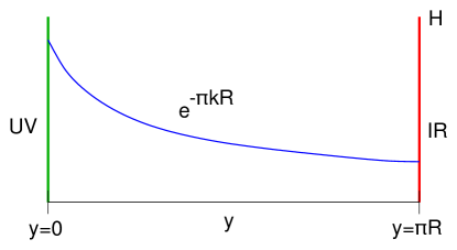
Figure 7: Schematic view of Randall-Sundrum spacetime. Two four-dimensional branes are separated in a fifth dimension which is denoted by the coordinate $y$. Masses on the infrared brane (IR) at $y=\pi R$ are reduced by a warp factor $\exp(-\pi kR)$ with respect to the same mass on the ultraviolet brane (UV). The quantity $R$ is the compactification radius of the fifth dimension and $k$ the spacetime curvature. The Higgs boson (H) is located on the IR brane. After [36].

The Planck mass $M_{\rm Pl}$ on the UV brane is $\approx\!10^{19}{\mathrm{\ Ge\kern-1.00006ptV}}$. On the IR brane it is only $1{\mathrm{\ Te\kern-1.00006ptV}}$ if $kR=11$. Effectively, fine-tuning of the radiative corrections to the Higgs mass is avoided by lowering the cut-off scale to $1{\mathrm{\ Te\kern-1.00006ptV}}$.

The fifth dimension is assumed to be periodic ($y\in(-\pi R,\pi R]$ with $y=-\pi R=\pi R$). All fields in the five dimensions (specified by five coordinates, $x^{\mu}$ and $y$) can be Fourier-expanded in a series of fields that depend only on $x^{\mu}$ [38]:

$$F(x^{\mu},y)=\sum_{n=-\infty}^{\infty}\ F_{n}(x^{\mu})e^{iny/R}\,.$$ (8)

The $F_{n}$ are the Kaluza-Klein (KK) [39, 40] excitations of $F$. Their masses $m_{n}$ are given by $m^{2}_{n}=n^{2}/R^{2}+m_{0}^{2}$ in which $m_{0}$ is the mass of the zero mode, the SM particle. For new KK particles to exist with masses of the order $1{\mathrm{\ Te\kern-1.00006ptV}}$, the radius $R$ has to be of the order $10^{-19}$ m.

At the LHC, the KK particle with the largest production cross section is the first excitation of the gluon. The KK gluon ($g_{\rm KK}$) is the most strongly coupled KK particle and is produced resonantly in the $s$-channel from two quarks. It is localised near the IR brane.

The SM particles live at different distances to the IR brane. The distances are free parameters of the theory and are adjusted manually to obtain the observed masses. The masses are determined by the overlap of the particle wave function with that of the Higgs boson which lives on the IR brane. The top quark is the SM fermion closest to the IR brane because it has the largest mass. Because the $g_{\rm KK}$ also lives near the IR brane, the consequence is that it prefers to decay to $t\bar{t}$ pairs. Shown in Figure 8 are distributions of the invariant mass of the $t\bar{t}$ pair in LHC collisions for different $g_{\rm KK}$ masses $m_{g_{\rm KK}}$ from $2$ to $7{\mathrm{\ Te\kern-1.00006ptV}}$. The width of the KK gluon is $\Gamma_{g_{\rm KK}}/m_{g_{\rm KK}}=17\%$. For these high resonance masses, the top quark $p_{\rm T}$ is $\approx\!m_{g_{\rm KK}}/2$ and the decay products are strongly collimated. Each top quark is therefore reconstructed as a single jet. Also shown is the background from SM $t\bar{t}$ production above which the signal clearly stands out (left panel). The dominating background is that from QCD dijet production (also referred to as multijet production) in which two partons scatter and produce two high $p_{\rm T}$ outgoing partons. After the QCD shower (gluon radiation and splitting) and fragmentation into hadrons, the final state consists of two or more jets. This background is shown in the right panel. It exceeds the signal by approximately one order of magnitude. To discover the signal, the multijet background has to be suppressed by analysing the internal structure of the jets.

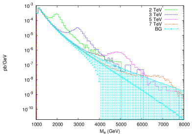
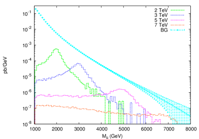
Figure 8: Invariant mass of $t\bar{t}$ pairs from decays of Kaluza-Klein gluons with different masses (generated with MadGraph). The distributions are compared to those from SM background (PYTHIA): a) $t\bar{t}$ production and b) multijet production for which the invariant mass of the leading $p_{\rm T}$ dijets is plotted ($|\eta^{\rm jet}|<0.5$ and leading $p_{\rm T}>500{\mathrm{\ Ge\kern-1.00006ptV}}$). The events are produced in LHC collisions at $\sqrt{s}=14{\mathrm{\ Te\kern-1.00006ptV}}$ and the background uncertainties correspond to $100\leavevmode\nobreak\ {\rm fb}^{-1}$. From [41].

3 Jet Structure

This section first briefly summarises the jet algorithms that are used in the results presented in this review. It then goes on to explain how jet structure differs for signal and background and introduces methods that exploit these differences. The susceptibility of jets to corrections from hadronisation and underlying event (UE) is discussed before methods are introduced that remove contributions from UE and pile-up from a jet (grooming). The analysis of the internal structure of jets is also referred to as substructure analysis, and the words structure and substructure are used synonymously in this context.

3.1 Jet algorithms

Jets are collimated sprays of particles and algorithms are used to define the geometrical size and the kinematics of the combined object. Conventionally, jets are used to get an estimate of the kinematics of partons that underwent a hard scattering process or which originate from the decay of a heavy particle. These high-energy partons surround themselves with a parton cloud by radiating gluons which can split into gluons or quark pairs. After hadronisation, the original parton momentum is distributed among many particles. A jet algorithm tries to find the original parton momentum by iteratively combining the momenta of nearby partons and in that sense reverse the parton splitting.

The most natural definition of a jet is based on a cone within which most of these particles are contained and the first jet algorithms used this concept [42, 43]. Another class of algorithms is based on the iterative recombination of neighbouring particles. These algorithms are easier made infrared-safe such that they arrive at the same hard jets when an additional soft gluon is added to the event. A discussion of jet algorithms can be found in [44]. All results discussed in this text use recombination algorithms.

All jet algorithms operate on a list of four-momenta, which can correspond to particles or detector quantities like tracks or calorimeter clusters, which will generically be referred to as constituents in the following. The combination algorithms merge two neighbouring constituents into one by combining their momenta. For the results discussed in this text, the $E$-scheme is used, in which the four-momenta are added, leading to massive jets. The objects that result from the merging are called protojets if they are not the final jets.

A distinction is made between inclusive and exclusive clustering: in the case of the former, a distance parameter $R$ is specified and the constituents or protojets $i$ and $j$ that are nearest in terms of a chosen distance scale are combined as long as $\Delta R_{ij}<R$. All resulting jets are separated by $\Delta R\geq R$. Exclusive clustering, on the other hand, ends when a specified number of jets has been obtained. Each jet is represented by a four-momentum vector, the $\theta$ and $\phi$ components of which define a jet axis.

The merging order is determined by the definition of the distance scale which specifies which neighbours $i,j$ are closest and hence will be merged next. Three common choices are

• the separation $\Delta R_{ij}$. In this case, the neighbours nearest in $(y,\phi)$ space are clustered first and the procedure is referred to as Cambridge/Aachen ($\mathrm{C/A}$) algorithm [45, 46, 47].

• $\min(p_{{\rm T},i},p_{{\rm T},j})\times\Delta R_{ij}$ ($k_{\rm T}$ algorithm [48, 49, 50]). Compared to $\mathrm{C/A}$, this clusters low $p_{\rm T}$ constituents earlier.

• $\min(1/p_{{\rm T},i},1/p_{{\rm T},j})\times\Delta R_{ij}$ (anti-$k_{\rm T}$ algorithm [51]). This clusters high $p_{\rm T}$ constituents earlier.

The $k_{\rm T}$ algorithm aims at reversing the angular ordered parton shower implemented in the HERWIG generator[52]. Jets reconstructed with the anti-$k_{\rm T}$ algorithm have a cone-like shape with the covered area given by $\approx\pi R^{2}$ whereas $\mathrm{C/A}$ and $k_{\rm T}$ jets tend to have more irregular shapes [51] as discussed in Section 7.1. Regardless of this fact, the distance parameter $R$ is commonly referred to as jet radius for all jet algorithms.

3.2 Jet structure in signal and background

To analyse differences in the (fat) jet structure between signal and background, it is instructive to compare the kinematics of the signal decay with QCD parton splitting processes. Schematic diagrams of these processes are shown in Figure 9.

Figure 9: Schematic diagrams of (left) the boosted decay of a particle $X$ to two quarks and (right) gluon radiation off a quark. In the right diagram, the fraction of the initial quark momentum retained by the quark is denoted $z$. The momentum fraction of the radiated gluon is $1-z$. Similarly, in the left diagram, the two quarks from the decay of $X$ carry momentum fractions $z$ and $1-z$. From [18].

It is of interest how the parent particle energy is distributed among the two outgoing particles. For gluon radiation in the collinear approximation, the probability that the quark retains a fraction $z$ of its momentum is given in leading order by the Altarelli-Parisi splitting function [53]

$$P_{gq}=\frac{4}{3}\frac{1+z^{2}}{1-z}\,.$$ (9)

Most of the gluons are therefore soft ($z\rightarrow 1$). For the signal, the decay is not as asymmetric. For example, the decay amplitude of the Higgs boson for $H\rightarrow b\bar{b}$ is flat in $z$ [18]. An efficient way to suppress background is therefore to reject configurations with large $z$. This is the idea behind the mass drop technique [4].

3.2.1 Mass drop

The mass drop (MD) criterion was developed to identify the decay $H\rightarrow b\bar{b}$ against a large multijet background [4]. The idea is to use boosted Higgs bosons for which the $b\bar{b}$ pair is collimated and contained inside a $\mathrm{C/A}$ fat jet. To find the subjets that correspond to the $b$-jets from the Higgs decay, the MD algorithm searches for a merging $i+j\rightarrow p$ for which the combined mass $m_{p}$ is significantly larger than either one of $m_{i}$ and $m_{j}$. Fat jets that originate from hard light quarks or gluons are unlikely to display this pattern because the splitting function (9) prefers soft radiation.

An iterative procedure is used because $\mathrm{C/A}$ clustering is by smallest angular separation and the last two protojets are not necessarily the wanted subjets. The algorithm starts with a fat jet $p$ and proceeds as follows:

1. the last clustering of $p$ is undone to obtain two protojets $i$ and $j$, labelled such that $m_{i}>m_{j}$. If $p$ cannot be split because it is a constituent then the fat jet is discarded. When applying the MD algorithm to calorimeter clusters, the detector resolution becomes relevant. In [54], the jet $p$ was also discarded if $\Delta R_{ij}<0.3$.

2. If $m_{i}/m_{p}<\mu$ and $\sqrt{v}\equiv\Delta R_{ij}\times\min(p_{{\rm T},i},p_{{\rm T},j})/m_{p}>\sqrt{v_{\rm cut}}$ then $i$ and $j$ are identified as the wanted subjets and the procedure ends. Otherwise the procedure continues with step 1 but now using the leading mass subjet as input ($p=i$). With $\Delta R_{ij}\approx 2m_{p}/p_{{\rm T},p}$, the second requirement reads $\min(p_{{\rm T},i},p_{{\rm T},j})/p_{{\rm T},p}\gtrsim\sqrt{v_{\rm cut}}/2$ and implies a minimum $p_{\rm T}$ for the softer protojet.

If two subjets can be found in this way then the original (fat) jet satisfies the MD criterion. In [4], the parameters are $\mu=0.67$, implying a mass drop of at least $33\%$, and $v_{\rm cut}=0.09$, i.e., the softer protojet has to have at least $\approx\!15\%$ of the combined $p_{\rm T}$.

By changing the parameters, the procedure can be adapted to the decay of other massive particles, like $W$ or $Z$ bosons or the top quark. One can also continue the mass drop procedure to identify two successive decays of massive particles, like in $t\rightarrow Wb\rightarrow qqb$.

3.2.2 $k_{\rm T}$ splitting scales

The splitting function (9) is also the motivation for cuts on $k_{\rm T}$ splitting scales [55] as explained in [44]: for quasi-collinear splitting to two partons $i$ and $j$, the squared invariant mass of the two partons is given by [56, 44]

$$m^{2}\approx p_{{\rm T},i}\,p_{{\rm T},j}\,\Delta R_{ij}^{2}\,.$$ (10)

Transverse momenta are used in this expression because jets are detected centrally in the LHC detectors where $p_{\rm T}$ is a good approximation of the full momentum. With $j$ denoting the softer parton and $p_{\rm T}=p_{{\rm T},i}+p_{{\rm T},j}$, (10) can be rewritten as

$$m^{2}\approx x\,(1-x)\,p_{\rm T}^{2}\,\Delta R_{ij}^{2}\,,$$ (11)

with the fraction $x=p_{{\rm T},j}/p_{\rm T}<0.5$. For a signal-like flat $x$ distribution with an average value of $0.25$, the mass is $m\approx 0.43\,p_{\rm T}\,\Delta R_{ij}$, which corresponds to (1). In the case of gluon radiation, $x$ is the $p_{\rm T}$ fraction carried by the gluon and corresponds to $1-z$ in (9).

The $k_{\rm T}$ splitting scale corresponds to the distance scale of the $k_{\rm T}$ algorithm and is given by

$$\sqrt{d_{ij}}\equiv\min(p_{{\rm T},i},p_{{\rm T},j})\,\Delta R_{ij}\,=x\,p_{\rm T}\,\Delta R_{ij}\approx\sqrt{\frac{x}{1-x}}\,m\,.$$ (12)

For gluon radiation, $x\rightarrow 0$ and the scale is small. For heavy particle decays with a more uniform $x$ distribution, this is not the case and a cut can be used to suppress the background. For a flat $x$ distribution, $\sqrt{d_{ij}}\approx 0.58\,m$. For top quark and vector boson decay, values of approximately half the parent particle mass are observed for $\sqrt{d_{ij}}$.

The $k_{\rm T}$ algorithm clusters high $p_{\rm T}$ objects late, so that the scale of the last merging, $\sqrt{d_{12}}$, and the one of the second-to-last merging, $\sqrt{d_{23}}$, are sensitive to the hard structure of the jet. For top quark decay, $\sqrt{d_{12}}$ is peaked near half the top quark mass and $\sqrt{d_{23}}$ is peaked near half the $W$ boson mass.

3.3 Jet energy corrections and contamination

The size of a jet is determined by the radius parameter $R$. The larger $R$, the larger the area in $(\eta,\phi)$ that is covered by the jet and the more underlying event (UE) energy will be picked up. The underlying event are the particles scattered in interactions that are not related to the hard scatter. These additional interactions are predominantly soft and the energies are small compared to those involved in the hard scatter. Nevertheless, these energies lead to a shift in the reconstructed jet energy compared to the energy of the hard scatter parton. The shift in $p_{\rm T}$ due to the UE is shown in Figure 10 (upper curves) as a function of the radius parameter $R$ for $\mathrm{C/A}$ jets with $55<p_{\rm T}<70{\mathrm{\ Ge\kern-1.00006ptV}}$ at the parton level in $gg\rightarrow gg$ scattering at the LHC with $\sqrt{s}=14{\mathrm{\ Te\kern-1.00006ptV}}$. The shift is evaluated using two different UE models (PYTHIA and HERWIG). It is approximately proportional to $R^{2}$ and for $R=1$ amounts to $\approx\!5{\mathrm{\ Ge\kern-1.00006ptV}}$ which is almost $10\%$ of the jet $p_{\rm T}$. The correction depends on the collision energy. For Tevatron $p\bar{p}$ collisions at $1.96{\mathrm{\ Te\kern-1.00006ptV}}$, the correction at $R=1$ is $1$–$2{\mathrm{\ Ge\kern-1.00006ptV}}$, depending on the model.

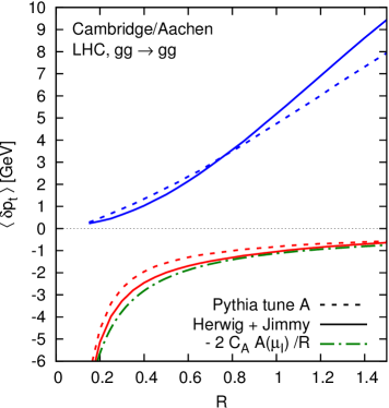
Figure 10: The correction from underlying event ($\delta p_{t}>0$) and hadronisation ($\delta p_{t}<0$) to the $p_{\rm T}$ of $\mathrm{C/A}$ jets as a function of the radius parameter $R$ for $gg\rightarrow gg$ scattering in $pp$ collisions at $\sqrt{s}=14{\mathrm{\ Te\kern-1.00006ptV}}$. The parton-level jet (after the parton shower) is required to have $55<p_{\rm T}<70{\mathrm{\ Ge\kern-1.00006ptV}}$. Shown are predictions from PYTHIA and from HERWIG with the JIMMY underlying event model and an analytical result for the hadronisation correction. From [57].

Another effect that depends on $R$ is the energy lost outside the jet by hadronisation. Hadronisation denotes the transition from coloured partons to colour-neutral hadrons. In this process, new partons emerge between colour-connected partons and the energy is in part re-assigned. If one compares a jet built from the partons with a jet of the same size built from the hadrons, the hadron jet has smaller energy (or $p_{\rm T}$) because some of the parton energy is lost in hadrons that are not captured in the jet. This loss is larger when the jet $R$ is smaller as shown in Figure 10 (lower curves). The $p_{\rm T}$ shift can be calculated analytically [57] and is approximately proportional to $1/R$. For $R=1$ the shift is $\approx-1{\mathrm{\ Ge\kern-1.00006ptV}}$ for $\mathrm{C/A}$ jets. In magnitude this shift is only $20\%$ of the UE shift which works in the opposite direction. The parameter $R$ that minimises the quadratic sum of the UE and hadronisation corrections is $R=0.41$ for quark jets and $R=0.54$ for gluon jets [57]. The standard jet sizes in the ATLAS and CMS experiments ($R=0.4$ and $R=0.5$, respectively) are driven by such optimisations. For fat jets ($R\geq 0.8$), the UE corrections are more important than for these standard jets.

Experimentally, jets are contaminated by pile-up which denotes the case that several hard interactions appear in the same event. This happens for two reasons: first, when the luminosity of the collider is sufficiently high (thereby giving a high probability for two hard interactions to occur in the same bunch crossing) and second, when the detector readout is slow such that events see remnants of signals from earlier events. These two contributions are sometimes referred to as in-time and out-of-time pile-up, respectively. This pile-up energy is larger than the UE contribution and scales with the area of the jet.

Jet substructure analysis tries to identify jets from top quark decay (or decay of other particles) inside a large (fat) jet. By exploiting kinematic relations between the decay partons, background can be suppressed. However, these relations no longer hold if the jet kinematics are changed by UE and pile-up contributions. In other words, these contaminations have to be removed to clearly “see” the jet substructure. Different techniques have been devised in this regard and are referred to as jet grooming.

3.4 Jet grooming

The process of jet grooming is the removal of unwanted constituents from a fat jet ($R\geq 0.8$). Different procedures have been developed and the ones relevant for this text are described in the following.

Trimming

Contributions from underlying event and pile-up are usually soft, i.e., have small energy, compared to those from the high-$p_{\rm T}$ hard scatter. The trimming procedure [58] creates $k_{\rm T}$ subjets with a radius parameter $R_{\rm sub}<R$ (typically $R_{\rm sub}=0.3$) using all constituents of the fat jet. Then the constituents of the subjets which carry less than a fraction $f_{\rm cut}$ (typically $5\%$) of the fat jet $p_{\rm T}$ are removed (trimmed) from the fat jet. This method does not correct for unwanted contributions that overlap with the hard subjets. It is therefore most useful for substructure variables that are very sensitive to soft contributions. An example is the fat jet mass, to which even low $p_{\rm T}$ constituents contribute significantly if they lie at large angles with respect to the hard constituents.

Pruning

The jet pruning procedure [59, 60] removes soft protojets at large angles in every jet clustering step. At every merging step of two protojets, $i+j\rightarrow p$, one calculates

$$z\equiv\min(p_{{\rm T},i},p_{{\rm T},j})/p_{{\rm T},p}$$ (13)

and discards the softer protojet if

$$z<z_{\rm cut}\quad{\rm and}\quad\Delta R_{ij}>D_{\rm cut}\,.$$ (14)

Otherwise the merging is applied. A protojet is therefore discarded if the other protojet carries much more $p_{\rm T}$ and the distance between the two protojets is large. The jet obtained using this conditional clustering is called a pruned jet. In [59] the cut values are $z_{\rm cut}=0.1$ for the $\mathrm{C/A}$ algorithm and $0.15$ for the $k_{\rm T}$ algorithm, and $D_{\rm cut}=m_{J}/p_{{\rm T},J}$ is the ratio of the mass of the unpruned jet to its $p_{\rm T}$.

Filtering

For filtering, the constituents of a jet are inclusively clustered using a filter radius that is small compared to the size of the jet. Only $N$ filter jets with the largest $p_{\rm T}$ are kept. The combination of a mass drop criterion with filtering was first used in [4] and has become known as mass drop filtering. It is illustrated in Figure 11 for $H\to b\bar{b}$. It is used in a number of substructure algorithms that have been suggested since, such as the HEPTopTagger [5, 19] which is described in Section 7.7.

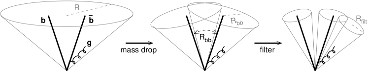
Figure 11: Illustration of the mass drop filtering technique. A fat jet containing the two bottom quarks from the decay $H\to b\bar{b}$ is broken down into two hard subjets (mass drop). The constituents of the subjets are reclustered with a radius parameter $R_{\rm filt}$ that is small compared to the subjet distance $R_{bb}$ and only the three highest $p_{\rm T}$ small-$R$ jets are kept (filtering). The third jet captures gluon radiation. From [4].

4 Experimental Setup

This section describes the devices used for the experimental results in this review.

4.1 LHC

The Large Hadron Collider (LHC) started colliding protons in December 2009. The results shown in this review are obtained using $pp$ collisions at centre-of-mass energies of $\sqrt{s}=7{\mathrm{\ Te\kern-1.00006ptV}}$ (2011) and $8{\mathrm{\ Te\kern-1.00006ptV}}$ (2012). The LHC was designed for $\sqrt{s}=14{\mathrm{\ Te\kern-1.00006ptV}}$ but operation at higher energies was not possible because cable connections between dipole magnets that were soldered at room temperature can develop high resistivity due to mechanical stress when cooled down to superconducting temperature. This can lead to electric arcs when the current is large. This happened on 19 September 2008 when a magnet quenched and an electric arc developed and punctured the enclosure that held the liquid helium. The helium expanded to the gaseous state and was released into the vacuum that thermally insulates the beam pipe. Upon expansion, the helium volume increased by a factor 1000 and the resulting pressure destroyed several magnets. The LHC had to be shut down for a year for repairs. After the restart, the magnet currents were kept below a safety threshold, thereby limiting the bending power and consequently the beam energy. Safely going to higher collision energies requires the replacement of all soldered connections with clamped splices. This work is ongoing since spring 2013 in the so-called Long Shutdown 1. After the replacement, the LHC is expected to collide protons with $\sqrt{s}=13$–$14{\mathrm{\ Te\kern-1.00006ptV}}$ starting in spring 2015.

In 2011 and 2012, the number of protons per bunch was $1.5$–$1.7\times 10^{11}$ with 1380 bunches in the machine [61]. The bunch separation was $50\,$ns. The instantaneous luminosity $\mathcal{L}$ reached values of $3.5\times 10^{33}\,$Hz/cm² in 2011 and $7.7\times 10^{33}\,$Hz/cm² in 2012.

The variable $\mu$ denotes the average number of inelastic $pp$ interactions per bunch crossing. It is calculated from the inelastic cross section $\sigma_{\rm inel}$, $\mathcal{L}$, and the average frequency $f_{\rm bunch}$ of bunch crossings in the LHC:

$$\mu=\sigma_{\rm inel}\ \frac{\mathcal{L}}{f_{\rm bunch}}\,.$$ (15)

The value used by ATLAS for the inelastic cross section is $71.5\,$mb at $\sqrt{s}=7{\mathrm{\ Te\kern-1.00006ptV}}$ and $73.0\,$mb at $8{\mathrm{\ Te\kern-1.00006ptV}}$. Figure 12 shows the $\mu$ distribution and the maximum instantaneous luminosity as a function of time. The average $\mu$ was 9.1 in 2011 and 20.7 in 2012.

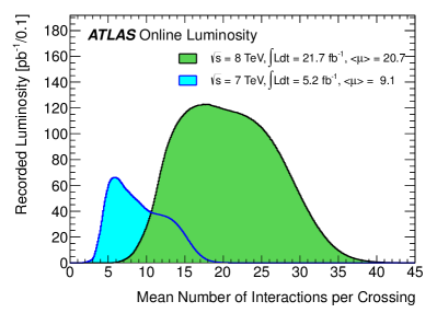
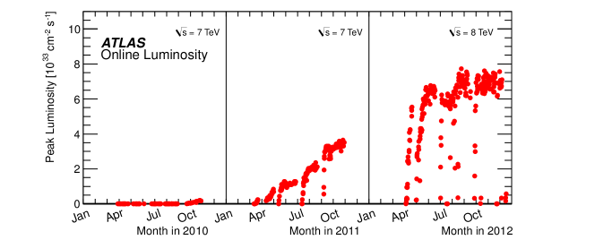
Figure 12: a) The luminosity-weighted distribution of the average number of inelastic $pp$ interactions per bunch crossing $\mu$ for 2011 and 2012 ATLAS data. b) The peak instantaneous luminosity as a function of time. From [62].

4.2 ATLAS

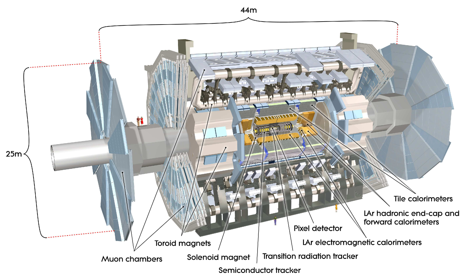
Figure 13: Schematic view of the ATLAS detector. From [63].

A schematic view of the ATLAS detector is shown in Figure 13. A full description of it can be found in [63, 64]. The parts relevant to the discussion of the results presented in this text are summarised below.

Closest to the interaction point is the inner tracking detector (ID) which consists of a silicon part (pixel and strips) and a transition radiation detector (TRT). The ID spans the full azimuthal range and $|\eta|<2.5$, and is immersed in a magnetic field of 2 T that is provided by a coil outside of the ID volume.

Hits in the ID are used to construct tracks of charged particles. The angular resolution of the ATLAS inner tracking detector for charged particles with $p_{\rm T}=10{\mathrm{\ Ge\kern-1.00006ptV}}$ and $\eta=0.25$ is $\approx 10^{-3}$ in $\eta$ and $\approx 0.3$ mrad in $\phi$ [63] with a track construction efficiency larger than $78\%$ for charged particles with $p_{\rm T}>500{\mathrm{\ Me\kern-1.00006ptV}}$ [65]. The momentum resolution for charged pions is $4\%$ for momenta $p<10{\mathrm{\ Ge\kern-1.00006ptV}}$, rising to $18\%$ at $p=100{\mathrm{\ Ge\kern-1.00006ptV}}$ [63].

Surrounding the magnet coil is the electromagnetic calorimeter (ECAL) which consists of a barrel part ($|\eta|<1.475$) and two endcap parts ($1.375<|\eta|<3.2$). It is a sandwich calorimeter with lead absorber plates and kapton electrodes immersed in liquid argon (LAr). The electrode cell size in $(\eta,\phi)$ varies from $0.025\times 0.025$ to $0.1\times 0.1$, depending on the layer and $\eta$. The hadronic calorimeter (HCAL) in the barrel ($|\eta|<1.7$) uses scintillating tiles while in the endcaps ($1.5<|\eta|<3.2$) the ECAL technology is used. HCAL cell sizes vary from $0.1\times 0.1$ to $0.2\times 0.2$.

Topological cell clusters are formed around seed cells with an energy $|E_{\rm cell}|>4\sigma_{\rm noise}$ by adding the neighbouring cells with $|E_{\rm cell}|>2\sigma_{\rm noise}$, and then all surrounding cells [66]. The minimal transverse size for a cluster of hadronic calorimeter cells is therefore $0.3\times 0.3$ and is reached if all significant activity is concentrated in a single cell. Two particle jets leave distinguishable clusters if each jet hits only a single cell and the jet axes are separated by at least $\Delta R_{\eta}=0.2$, so that there is one empty cell between the two seed cells. The finest angular resolution of the hadronic calorimeter is therefore $\Delta R_{\eta}=0.2$ which is much coarser than the resolution of the tracking detector given above.

The LAr system is slow and signals from several inelastic $pp$ interactions can overlap. The signal from one of the cells in the barrel is shown in Figure 14. A long tail of several hundred ns is visible. With a bunch spacing of $50\,$ns and many interactions per bunch crossing, it is likely that the same cell again detects activity while signals from previous events are still being processed. The bipolar shape was designed such that the negative signal from earlier events cancels pile-up signals from current events. This cancellation holds for $\mathcal{L}=10^{34}\,$Hz/cm² at $\sqrt{s}=14{\mathrm{\ Te\kern-1.00006ptV}}$. For other luminosities and collision energies the system is susceptible to (out-of-time) pile-up.

Figure 14: Amplitude vs. time for a triangular current pulse in one of the ATLAS LAr calorimeter cells. From [63].

Muons are detected in a spectrometer that covers $|\eta|<2.7$ with a toroidal magnetic field that is perpendicular to the momentum of central muons.

4.3 CMS

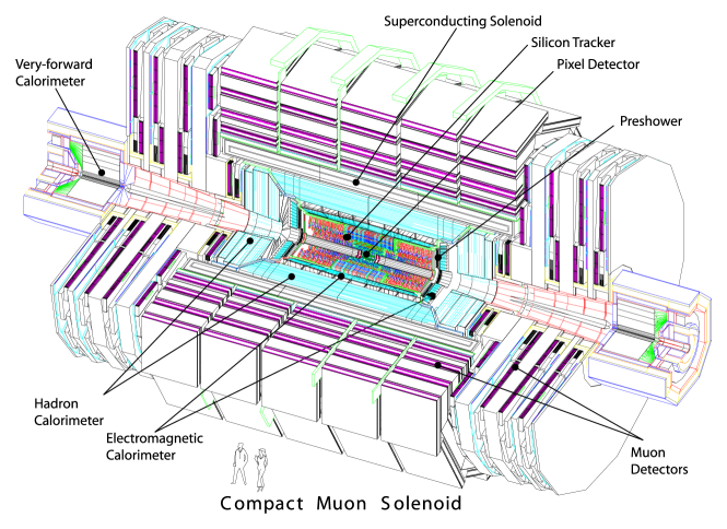
Figure 15: Schematic view of the CMS detector. From [67].

The CMS detector is shown schematically in Figure 15. A detailed description is given in [67]. Tracking is provided by silicon pixel and strip detectors inside a 3.8 T magnetic field. The magnet coil has a diameter of six metres and surrounds the barrel and endcap calorimeters ($|\eta|<3$). The ECAL consists of scintillating lead tungstate crystals. The HCAL is of a sandwich type with alternating layers of brass and scintillator tiles. Outside the magnet coil are gaseous detectors that are used to measure muons. The use of scintillator technology for the calorimeters makes the CMS data less susceptible to pile-up than ATLAS data.

To reconstruct particles, CMS uses the particle flow approach, which correlates information from the inner tracking detector, the calorimeters, and the muon detector. Clusters are reconstructed separately in the preshower detector, the ECAL, and the HCAL. Tracks and clusters are linked if they can be geometrically matched. The tracks are extrapolated to the calorimeter and if the end point is within the cluster or within a margin of one cell around the cluster, a track-cluster link is established. Clusters in different calorimeters are linked if the cluster in the finer calorimeter is within the cluster of the coarser calorimeter.

The particle flow algorithm [68] first reconstructs muons, then electrons and Bremsstrahlung photons, and finally charged hadrons. The remaining entries are then taken to be photons and neutral hadrons. After every step, the detector entries associated with a particular particle type are removed before continuing with the next type. Muons are identified through a global fit of hits in the inner detector and the muon detector. The energy left by muons is $0.5(5){\mathrm{\ Ge\kern-1.00006ptV}}$ in the ECAL and $3(3){\mathrm{\ Ge\kern-1.00006ptV}}$ in the HCAL. Electrons are found in a fit that includes emission of Bremsstrahlung photons at layers of the tracking detector and cuts on calorimeter variables. Charged hadrons are identified by comparing the $p_{\rm T}$ of a track with the calibrated energy of the associated cluster (track-cluster link). If the $p_{\rm T}$ and the energy are compatible, a charged hadron is reconstructed using the track $p_{\rm T}$ and the mass of a charged pion. A complication arises when several ECAL clusters are associated to the track. These clusters can correspond to the electromagnetic part of a hadronic shower, in which case they should be included in the charged hadron energy, or to photons. The clusters are ordered in distance from the extrapolated track position and the energy of the closest clusters is added to the track-associated cluster until the $p_{\rm T}$ of the track is reached. If the cluster energy exceeds the track $p_{\rm T}$ then a photon is reconstructed with the energy measured in the ECAL and a neutral hadron with the HCAL energy. The preference is given to photons because they constitute on average $25\%$ of the jet energy while only $10\%$ is carried by neutral hadrons and not all of their energy is deposited in the ECAL. The cluster calibration is obtained from simulation and is validated using test-beam data and collision data with isolated charged hadrons [69]. The photon energy is validated using $\pi^{0}$ decays [69].

5 Monte Carlo Generation and Detector Simulation

This section briefly describes the simulation tools that are used to obtain predictions for jet substructure. The degree to which jet substructure observables can be predicted using generated events and a simulation of the detector response greatly determines their usefulness in physics analyses. The precision of these predictions enters as a systematic uncertainty in analyses.

5.1 Monte Carlo generators

Different Monte Carlo (MC) generators are used to obtain predictions at the particle level. The multipurpose generator PYTHIA is used in versions 6 [70] and 8 [71]. PYTHIA calculates hard $2\rightarrow 2$ parton scattering at leading order (LO) in perturbative QCD. Higher orders are emulated using a parton shower [72]. In version 6, the evolution variable in the parton shower can be chosen to be either virtuality (mass) or transverse momentum. In version 8, the evolution is in transverse momentum and dipole showering is possible for the final state. The partons are hadronised using Lund string fragmentation [74]. PYTHIA has a multiple interactions model for the underlying event (UE). The hadronisation and UE model parameters are tuned to minimum bias data. ATLAS tunes are described in [75, 76].

Another LO generator is HERWIG [77, 52, 78]. It uses an angular-ordered parton shower to emulate higher order effects. The final state partons are hadronised using cluster fragmentation [79]. HERWIG is commonly combined with the JIMMY generator [80] for multiple interactions. The hadronisation and UE parameters are tuned to data, for example in [81]. HERWIG++ [82] is a replacement for HERWIG and is written in C++. It includes an underlying event model [83].

MC@NLO [84] was the first program to combine next-to-leading order (NLO) QCD calculations with a parton shower without double-counting. It uses the HERWIG parton shower. POWHEG [85] also combines an NLO matrix element with a parton shower but any parton shower program can be interfaced.

In the NLO MC programs, the matrix element calculations are limited to a small number of outgoing particles. Multileg generators were created that calculate final states with more particles at LO. An example is AMEGIC++ [86] which was integrated in the SHERPA framework [87, 88] to supplement it with a parton shower and evolve the events to the hadron level. SHERPA uses virtuality-ordered parton showering, cluster fragmentation, and an underlying event model similar to that of PYTHIA. Other multileg generators are ALPGEN [89] and MadGraph [90, 91]. The program AcerMC [92] uses matrix elements from MadGraph and has optimised phase space sampling for a selection of SM processes.

5.2 Detector simulation

Detectors for particle physics experiments are very complicated setups. To correct experimental effects introduced through the measurement apparatus, the generated particles at the stable hadron level are passed through a simulation of a detector.

The best detector simulation is obtained when every interaction of each particle with the detector material is calculated separately, usually with the program GEANT4 [93]. This type of simulation is referred to as full simulation and requires detailed knowledge about the detector geometry and material. Pile-up is simulated by overlaying the hard scattering event with minimum bias events that are produced using PYTHIA. All predictions in this review use full simulation, except where indicated.

Full simulation is part of the intellectual property of the detector collaboration and usually not available to non-collaborators. Without access to the full simulation, phenomenologists use generic detector simulations to estimate the impact of detector effects. The generic simulations are based on simplified virtual versions of existing detectors such as ATLAS or CMS. Key figures like geometry, acceptance, granularity, tracking and calorimeter resolutions are taken from information published by the collaborations. In this way, a decent simulation is possible that achieves predictions within approximately $20\%$ of the real response. Examples of generic simulation frameworks are AcerDET [94], Delphes [95, 96], and PGS [97].

6 Jet Reconstruction

This section summarises jet reconstruction and calibration in ATLAS and CMS. Both collaborations use the FastJet program [98, 99] to cluster input objects into jets.

6.1 Jets in the ATLAS detector

Different stages in the construction and use of ATLAS jets are discussed below. First the inputs to jets are described, followed by summaries of the calibration of calorimeter jets and the evaluation of systematic uncertainties associated with the modelling of the jet response in simulation. Finally, the procedure used to identify jets originating from hard bottom quarks ($b$-jets) in ATLAS is discussed.

6.1.1 Inputs to jet construction

For the analysis of ATLAS data, jets are formed using the four-momenta of different input quantities. At the particle level, jets are obtained from all particles with a lifetime of at least 10 ps. These particle jets are used to calibrate the calorimeter jet response.

The standard detector level jets in ATLAS are built from topological calorimeter clusters with positive energy. Depending on the cluster energy density, likelihoods are calculated that the cluster results from electromagnetic or hadronic interactions and a correction is applied to the cluster energy based on simulations of single pion interactions with the calorimeter (a process called local cluster weighting, LCW). The clusters are taken to be massless.

Jets are also constructed using tracks. The resulting track jets are used to validate the calibrations obtained through calorimeter simulation. The tracks have to fulfil quality requirements such as a minimal number of hits in the silicon detector and small longitudinal and transverse impact parameters with respect to the hard scattering vertex which is chosen to be the one with largest $\sum p_{\rm T,track}^{2}$. For jet reconstruction, tracks must have $p_{\rm T}>500{\mathrm{\ Me\kern-1.00006ptV}}$ and the mass is set to the charged pion mass to obtain a four-momentum for jet clustering.

6.1.2 Jet calibration

The standard ATLAS jets that are used in conventional analyses are constructed with the anti-$k_{\rm T}$ algorithm with $R=0.4$ or $R=0.6$. A long chain of sophisticated methods is applied to calibrate the jets and to derive the systematic uncertainties associated with the simulation of the jets [100, 101]. The methods are refined for every data-taking year because higher statistical measurement precision allows the application more data-driven approaches. Only parts of the full chain are used for the substructure jets, i.e., fat jets and their subjets, because of manpower constraints. The uncertainties are therefore larger for the substructure jets. Only the substructure jet calibrations and uncertainties are discussed in the following.

The jets are calibrated using a simulation of the calorimeter jet response by comparing the energy and pseudorapidity of a particle jet to that of a matching calorimeter cluster jet [100]. The mass of fat jets is calibrated in an analogous way. The procedure matches particle jets to calorimeter jets geometrically and determines the distribution of the ratio of the reconstructed quantity (energy, pseudorapidity, mass) and the particle level quantity. A Gaussian fit is performed to the core of the distribution to obtain a correction factor. Simulations of multijet events are used for the correction. Fat jets are required to be isolated (typically $\Delta R_{\eta}>1.0$) and the particle/detector level jet matching uses $\Delta R_{\eta}<0.3$. For subjets, the isolation criterion is removed and a tighter matching is used ($\Delta R_{\eta}<0.1$).

Different approaches are used for 2011 and 2012 ATLAS data to suppress pile-up contributions. For the 2011 substructure jets, an implicit average pile-up correction is applied by overlaying minimum bias events with the hard multijet events that are used to calculate the detector-to-particle-level correction factor. In the correction to the particle level, pile-up due to earlier collisions (and the slow calorimeter) is therefore removed because it is not part of the particle level jet. The 2012 procedure is described in [102]: before calibrating the subjets, energy depositions that originate from pile-up are removed to a large extent by applying an area correction [103] to each jet [104]. In this correction, the product $\rho\times A_{\rm T}$ is subtracted from the jet $p_{\rm T}$, in which $\rho$ is the median $p_{\rm T}$ density of the event and $A_{\rm T}$ is the transverse component of the jet area which is evaluated using ghost association [105]. The median $p_{\rm T}$ density is defined as

$$\rho={\rm median}\left\{p_{{\rm T},i}^{\rm jet}/A^{\rm jet}_{i}\right\}$$ (16)

in which the index $i$ enumerates the jets found when clustering the event with the $k_{\rm T}$ algorithm with $R=0.4$ and requiring positive jet energy but no minimal jet $p_{\rm T}$.

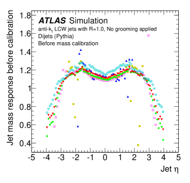
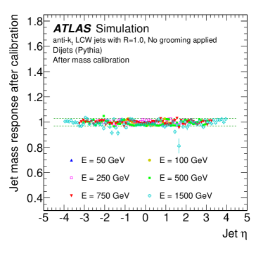
Figure 16: Mass response of the ATLAS calorimeter for anti-$k_{\rm T}$ $R=1.0$ jets (a) before and (b) after jet mass calibration. The response is defined as the mean of Gaussian fit to the core of the ratio of the reconstructed jet mass to the mass of a geometrically matched particle jet. From [106].

The 2011 ATLAS mass response for anti-$k_{\rm T}$ $R=1.0$ fat jets before and after calibration is shown as a function of $\eta$ in Figure 16. Before calibration, the mass in the central region ($|\eta|<2$) is too large by $10$–$20\%$ because of pile-up contributions and noise. After correction, the particle jet mass is reconstructed within $3\%$ for all energies.

The $\mathrm{C/A}$ subjets used in the HEPTopTagger are calibrated as follows. To be able to provide calibrations for the filtering step with its dynamic distance parameter $R_{\rm filt}$, the calibration constants are derived for jets with $R=0.2,0.25,\ldots,0.5$. When applying the calibration in the HEPTopTagger, the constants are used that correspond to $R_{\rm filt}$ or the next largest $R$ if no constants exist for the dynamically calculated $R_{\rm filt}$.

6.1.3 Validation of jet calibration using tracks

Uncertainties in the jet calibration are determined from the quality of the modelling of the calorimeter jet $p_{\rm T}$ and mass. The direct ratio $p_{\rm T}^{\mathrm{jet}}({\rm MC})/p_{\rm T}^{\mathrm{jet}}({\rm data})$ is sensitive to mis-modelling of jets at the particle level (the same is true for the mass). To reduce this effect, the calorimeter jet $p_{\rm T}$ is normalised to the $p_{\rm T}$ of tracks associated with the jet (or to the $p_{\rm T}$ of a geometrically matched track jet) because the uncertainty on the track $p_{\rm T}$ is small compared to the uncertainty on the calorimeter energy.

To evaluate the calorimeter-associated uncertainties of fat jets, jets built from tracks are geometrically matched to calorimeter jets ($\Delta R_{\eta}<0.3$). The ratios $r^{p_{\rm T}}_{\rm track\,jet}$ and $r^{m}_{\rm track\,jet}$ are defined as the calorimeter-to-track ratios

$$r^{p_{\rm T}}_{\rm track\,jet}=\frac{p_{\rm T}^{\mathrm{jet}}}{p^{\mathrm{track\;jet}}_{\rm T}}\,,\qquad r^{m}_{\rm track\,jet}=\frac{m^{\rm jet}}{m^{\mathrm{track\;jet}}}\,.$$ (17)

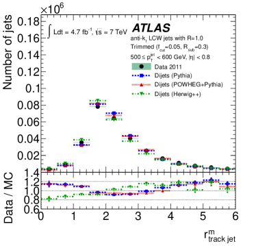
Figure 17: Ratio of the calorimeter jet mass to the mass of geometrically matched track jets for (a) $\mathrm{C/A}$ $R=1.2$ jets without grooming and (b) anti-$k_{\rm T}$ $R=1.0$ jets, trimmed with $f_{\rm cut}=5\%$ and $R_{\rm sub}=0.3$. From [106].

Figure 17 shows $r^{m}_{\rm track\,jet}$ for ungroomed $\mathrm{C/A}$ fat jets and trimmed anti-$k_{\rm T}$ fat jets ($f_{\rm cut}=5\%$, $R_{\rm sub}=0.3$). The ratios are larger than unity because only charged particles contribute to the track jets. The distribution for the ungroomed $\mathrm{C/A}$ jets is well described by the simulations. The ratio for the trimmed jets is described within $20\%$. Data-to-simulation double ratios are defined using the average values of $r^{p_{\rm T}}_{\rm track\,jet}$ and $r^{m}_{\rm track\,jet}$:

$$R_{\rm track\,jet}^{p_{\rm T}}=\frac{\langle r^{p_{\rm T}}_{\rm track\,jet}({\rm data})\rangle}{\langle r^{p_{\rm T}}_{\rm track\,jet}({\rm MC})\rangle}\,,\qquad R_{\rm track\,jet}^{m}=\frac{\langle r^{m}_{\rm track\,jet}({\rm data})\rangle}{\langle r^{m}_{\rm track\,jet}({\rm MC})\rangle}\,.$$ (18)

The double ratio is calculated in bins of $p_{\rm T}$ and $\eta$ and for different Monte Carlo generators. The deviation from unity is used as an estimate of the systematic simulation uncertainty. The uncertainty is in the range of $4$–$8\%$, depending on $p_{\rm T}$, $\eta$, the jet algorithm, and on whether the jet is trimmed or not. This uncertainty includes uncertainties related to the tracking efficiency which arise from the imperfect knowledge of the material distribution in the tracking detector.

To evaluate the subjet energy scale uncertainty, tracks are matched to calorimeter jets using ghost association [103, 105] as follows. For every track, a ghost is created by setting the $p_{\rm T}$ to a small value ($10$ eV) and using the track $\eta$ and $\phi$ at the calorimeter surface. The energy of the ghost is set to $1.001$ times its momentum to ensure a positive ghost mass. The ghost tracks are added to the calorimeter jet clustering but do not change the jet because their energy is negligible. If the ghost track ends up in the jet then the original track is taken to be associated with the jet. The jets are required to lie within $|\eta|<2.1$ to ensure coverage of the associated tracks by the tracking detector. The impact of pile-up is reduced because only tracks coming from the hard scattering vertex are used. The ratio $r_{\rm trk}$ is defined as the ratio of the sum of the $p_{\rm T}$ of the tracks associated with the jet to the $p_{\rm T}$ of the jet:

$$r^{\rm subjet}_{\rm trk}\equiv\frac{\sum p_{\rm T}^{\mathrm{track}}}{p_{\rm T}^{\rm subjet}}$$ (19)

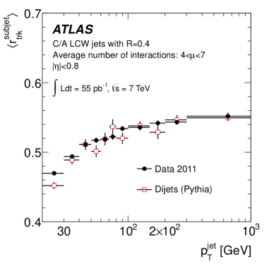
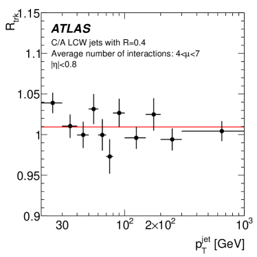
Figure 18: Comparison of the calibrated Cambridge/Aachen $R=0.4$ calorimeter jet $p_{\rm T}$ with the $p_{\rm T}$ of tracks matched to the jet for ATLAS data recorded in 2011 and for multijet simulations from PYTHIA. The average number $\mu$ of inelastic $pp$ interactions per bunch crossing ranges from $4$ to $7$. (a) The average ratio $r_{\rm trk}$ as a function of the calibrated jet $p_{\rm T}$. (b) The double ratio $R_{\rm trk}={\langle r^{\rm subjet}_{\rm trk}\rangle}_{\rm data}/{\langle r^{\rm subjet}_{\rm trk}\rangle}_{\rm MC}$. The horizontal line indicates the uncertainty-weighted average. From [106].

Figure 18a shows the average $r_{\rm trk}$ as a function of jet $p_{\rm T}$ for $\mathrm{C/A}$ $R=0.4$ jets with calibrated $p_{\rm T}$ between $30$ and $40{\mathrm{\ Ge\kern-1.00006ptV}}$ for $4<\mu<7$. The track-to-calorimeter $p_{\rm T}$ ratio $r^{\rm subjet}_{\rm trk}$ would be equal to 2/3 if all produced particle were pions because the tracking detector responds only to charged pions. However, this ratio is changed by the production of other mesons and baryons. The fraction of charged particles is well simulated by PYTHIA as evident from the description in Figure 18a.

The double ratio $\displaystyle R_{\rm trk}\equiv{\langle{r^{\rm subjet}_{\rm trk}}\rangle}_{\rm data}/{\langle{r^{\rm subjet}_{\rm trk}}\rangle}_{\rm MC}$ is shown in Figure 18b. The largest deviation from unity is $4\%$ at low $p_{\rm T}$ with a statistical uncertainty of $1\%$. No rise of the uncertainty with jet $p_{\rm T}$ is observed. Similar results are obtained when varying the jet radius parameter between $0.2$ and $0.5$ and for high pile-up conditions ($13<\mu<15$). Including systematic uncertainties on the tracking performance, the subjet energy uncertainty varies between $2.3\%$ and $6.8\%$, depending on $p_{\rm T}$, $\eta$, and the jet radius.

A sample of semileptonically decaying $t\bar{t}$ pairs is used to study the energy scale in events with heavy flavour jets and a boosted topology in which subjets are close-by. Events are selected from the 2011 dataset as described in Section 9.1 with a $\mathrm{C/A}$ $R=1.5$ jet with $p_{\rm T}>200{\mathrm{\ Ge\kern-1.00006ptV}}$. According to simulation, $\approx\!50\%$ of the events have semileptonically $t\bar{t}$ pairs in which the hadronically decaying top quark has $p_{\rm T}>200{\mathrm{\ Ge\kern-1.00006ptV}}$ and the remaining events are dominated by $W\!$+jets production. The subjet energy uncertainty determined from this sample varies between $2.4\%$ and $5.7\%$. ATLAS members can find a detailed description of the calibration of the HEPTopTagger subjets and the evaluation of the energy scale and $p_{\rm T}$ resolution uncertainties in [107, 108].

6.1.4 $b$-jets

The $b$-tagging algorithm MV1 used for the results presented in this article is based on a neural net that combines information from significances of impact parameters and decay length, the total invariant mass of the tracks at the vertex, the fraction of the total jet energy carried by tracks that is associated with tracks from the vertex, the multiplicity of two track vertices, and the direction of the $b$-hadron determined from the subsequent decay vertex of the charmed hadron. The algorithm tags anti-$k_{\rm T}$ $R=0.4$ jets.

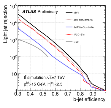
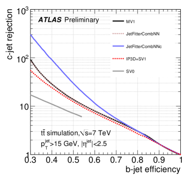
Figure 19: The performance of $b$-tagging algorithms in ATLAS in simulated $t\bar{t}$ events. (a) Rejection of light quark jets vs. efficiency and (b) Rejection of charmed jets vs. efficiency. From [109].

The MV1 efficiency is shown in Figure 19 as a function of the rejection of light quark jets and charmed jets for simulated $t\bar{t}$ events. Rejection is defined as the inverse of the mis-tagging rate (fake rate). At an efficiency of $70\%$, the fake rate is $\approx\!0.8\%$ for light quark jets and $\approx\!20\%$ for $c$-jets.

Systematic simulation uncertainties on the $b$-tagging efficiency and on the mis-tagging rate are obtained from data using different methods. The most precise method determines the uncertainty for jets with $p_{\rm T}<300{\mathrm{\ Ge\kern-1.00006ptV}}$ from $t\bar{t}$ events [110] and fits the observed $b$-tag multiplicity. The study is carried out using a semileptonic $t\bar{t}$ selection and a leptonic selection. The flavour composition before the tag is obtained from simulation. The expected number of $b$-tags is given by the product of the number of signal and background jets of a particular flavour with the efficiency to tag this jet. The mis-tag rates are taken from simulation but with data-driven scale factors applied [110]. The efficiency is obtained through a fit to the measured $b$-tag multiplicity. If one would consider only one data sample then the equation could be solved for the efficiency instead of fitting. However, several channels are considered: $e$+jets, $\mu$+jets, $ee$, $\mu\mu$, and $e\mu$. The $t\bar{t}$ production cross section is known to $10\%$ and the normalisation is left floating in the fit within this uncertainty. Similarly, the background normalisation is determined in the fit.

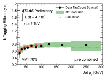
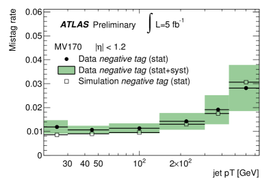
Figure 20: Efficiency and mis-tag rate of the MV1 algorithm operating at the $70\%$ working point for anti-$k_{\rm T}$ $R=0.4$ jets as a function of the jet $p_{\rm T}$. (a) The $b$-tag efficiency obtained from a fit of the $b$-tag multiplicity in a selection of $t\bar{t}$ events. The simulation is from MC@NLO. From [110]. (b) The mis-tag rate obtained from negative impact parameters and decay lengths. The simulation is from PYTHIA. From [111].

The obtained MV1 $b$-tag efficiency is shown in Figure 20a as a function of the anti-$k_{\rm T}$ $R=0.4$ jet $p_{\rm T}$ for the $70\%$ efficiency working point settings. The efficiency is $55\%$ at $p_{\rm T}=25{\mathrm{\ Ge\kern-1.00006ptV}}$ and reaches $75\%$ for $p_{\rm T}=100{\mathrm{\ Ge\kern-1.00006ptV}}$. The relative uncertainty in the $p_{\rm T}$ range $200$–$300{\mathrm{\ Ge\kern-1.00006ptV}}$ is $25\%$. A different method that uses a kinematic fit to the $W$ boson and top quark masses to determine the $b$-jet yields an uncertainty of $10\%$ in this $p_{\rm T}$ range but has slightly larger errors at low $p_{\rm T}$. The uncertainty for $200$–$300{\mathrm{\ Ge\kern-1.00006ptV}}$ is assumed to be valid also for larger $p_{\rm T}$ but additional uncertainties are added in quadrature as discussed below. The efficiency decreases with $p_{\rm T}$ for $p_{\rm T}>200{\mathrm{\ Ge\kern-1.00006ptV}}$.

The rate at which light quark jets are tagged by the MV1 algorithm has been studied in [111]. Mis-tags occur from fake secondary vertices which result from tracks being reconstructed at displaced locations due to the finite tracking resolution, from material interactions, or from long-lived particles (e.g., $K^{0},\Lambda$). For the former of these sources of mis-tags, the signed impact parameter distribution and the signed decay length distribution should be symmetric around zero and a mis-tag rate is calculated from the negative tail of these distributions in multijet events. This rate is then corrected for contributions from material interactions and long-lived particles which occur predominantly at positive impact parameters and decay lengths. The measured mis-tag rate is shown in Figure 20b. It is $1\%$ for jet $p_{\rm T}<100{\mathrm{\ Ge\kern-1.00006ptV}}$ and rises to $3\%$ for $750{\mathrm{\ Ge\kern-1.00006ptV}}$. The uncertainty is $\approx\!30\%$ for $300$–$450{\mathrm{\ Ge\kern-1.00006ptV}}$.

Additional uncertainties on the $b$-tagging efficiency and fake rate are estimated using simulation and are added in quadrature to the uncertainties determined at lower $p_{\rm T}$. The largest contribution comes for the loss of tracking efficiency in the core of jets where adjacent hits created by two charged particles in the pixel detector are merged such that only one track is reconstructed.This effect is relevant for jet $p_{\rm T}>500{\mathrm{\ Ge\kern-1.00006ptV}}$ and is propagated to the $b$-tagging algorithm using simulation. The resulting uncertainty on the $b$-tagging can be as large as $50\%$ for $p_{\rm T}>800{\mathrm{\ Ge\kern-1.00006ptV}}$.

6.2 Jets in the CMS detector

The CMS analysis discussed in this article uses jets reconstructed from charged hadrons reconstructed with the particle flow approach (cf. Section 4.3). The hadrons have to be consistent with originating from the hard scattering vertex (the primary vertex with the largest $\sum p_{\rm T,track}^{2}$) to reduce pile-up contributions.

The jets are calibrated in different stages [112]. First, the jet area correction is applied to reduce pile-up contributions. The method is based on the multiplication of the jet area with the average $p_{\rm T}$ density in the event as discussed for ATLAS jets in Section 6.1.2. Then the jet energy is corrected using simulation by comparing the jet to a geometrically matched particle jet ($\Delta R_{\eta}<0.25$). The correction for anti-$k_{\rm T}$ $R=0.5$ jets is $+10\%$ at $p_{\rm T}=20{\mathrm{\ Ge\kern-1.00006ptV}}$ and smaller at higher $p_{\rm T}$. The smallness of the correction is due to the use of the track $p_{\rm T}$ in the particle flow algorithm. For comparison, the correction of ATLAS $\mathrm{C/A}$ $R=0.4$ jets which are calculated from clusters calibrated to the response of single pions (LCW) is $+33\%$ when a similar jet area correction has been applied before [102]. Next, the jets are intercalibrated in $\eta$ using the $p_{\rm T}$ balance of jets in the central region ($|\eta|<1.3$) with more forward jets. The measured $p_{\rm T}$ balance in $\gamma$+jets events and $Z\!$+jets events with $/{\!\!\!\!E_{\rm T}}$ is used to correct for small differences in simulation and data (missing transverse energy projection fraction method, MPF [113]). This last correction factor is calculated for the central region.

The full jet energy correction factor is shown in Figure 21a for anti-$k_{\rm T}$ $R=0.5$ jets with $p_{\rm T}=50{\mathrm{\ Ge\kern-1.00006ptV}}$. It is less than $1.13$ for $|\eta|<2.7$. Also shown are the correction factors for jets constructed from calorimeter towers and using the Jet-Plus-Track (JPT) algorithm [114], which corrects the energy of calorimeter jets using track jets. The corrections for the JPT algorithm are smaller in the central region with uncertainties similar to the particle flow approach. The correction rises for $|\eta|>2$ because the calorimeter jets extend beyond the acceptance of the tracking detector. The correction factor for the calorimeter tower jets is larger than $1.5$ for $|\eta|<2$ and reaches $\approx\!2$ in the barrel-to-endcap transition at $|\eta|=1.3$.

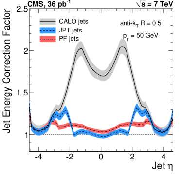
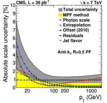
Figure 21: Calibration of the energy of CMS anti-$k_{\rm T}$ $R=0.5$ jets. (a) The energy calibration factor at jet $p_{\rm T}=50{\mathrm{\ Ge\kern-1.00006ptV}}$ as a function of $\eta$ for jets constructed using particle flow (PF), calorimeter towers (CALO), and the Jet-Plus-Track algorithm (JPT). (b) The energy scale uncertainty for particle flow jets as a function of $p_{\rm T}$. From [112].

Uncertainties on the jet energy originate from a variety of sources. The largest contribution at low $p_{\rm T}$ results from the uncertainty on the $p_{\rm T}$ density in the pile-up offset correction. The photon energy scale is known to $\approx\!1\%$. A $1\%$ uncertainty at $p_{\rm T}=20{\mathrm{\ Ge\kern-1.00006ptV}}$ results for the MPF method from leakage of forward particles ($|\eta|>5$), the uncertainty of which is taken from simulation to be $50\%$ of the difference between the true response and the MPF response. The jet energy scale uncertainty is shown in Figure 21b. It is $5\%$ at $p_{\rm T}=20{\mathrm{\ Ge\kern-1.00006ptV}}$ and smaller than $3\%$ for $p_{\rm T}>50{\mathrm{\ Ge\kern-1.00006ptV}}$.

7 Boosted Top Quark Finders

Boosted top quark identification algorithms operate on fat jets which, for signal, are supposed to contain all decay products of the top quark. The non-top contributions inside the fat jet are removed using jet grooming procedures. If the remaining constituents fulfil certain kinematic requirements (such as the jet mass being compatible with the top quark mass) they form a top quark candidate. The algorithms are referred to as top taggers, because of their ability to tag labels top or non-top to the fat jets.

The taggers can be classified into two categories. The first class, commonly called energy flow taggers, uses the spatial distribution of the fat jet constituents and their energies to calculate cut variables. The second approach is to explicitly reconstruct the 3-prong top quark decay structure in the form of subjets inside the fat jet. The algorithms and variables used so far in ATLAS and CMS are introduced in the following. Their grouping into the two categories is as follows:

energy flow:	jet mass, $k_{\rm T}$ splitting scales, $N$-subjettiness, Top Template Tagger
3-prong:	Johns Hopkins Top Tagger, CMS Top Tagger, HEPTopTagger

A detailed review of top taggers is given in [8]. The top taggers in the present article aim at reconstructing hadronically decaying top quarks.

7.1 Jet mass

The mass of a jet is an inclusive substructure variable. The structure information is encoded in a single number that results from a convolution of energy deposits and angles. The mass of a jet that contains all top decay products can have a mass greater than the top quark mass $m_{t}$ because of contributions from other particles. The application of grooming techniques is particularly useful here.

To illustrate the distributions and the effect of grooming, simulated signal events are used with pairs of top quarks, and simulated background events from multijet production. The top quarks result from the decay of a hypothetical new particle, the topcolor $Z^{\prime}$ introduced in Section 2.4, of mass $1.6{\mathrm{\ Te\kern-1.00006ptV}}$ into $t\bar{t}$. The top quarks are back-to-back in $\phi$ and their $p_{\rm T}$ is large and peaked at $800{\mathrm{\ Ge\kern-1.00006ptV}}$ (Jacobian peak). Two different algorithms are used to construct fat jets: the anti-$k_{\rm T}$ algorithm with $R=1.0$ and the $\mathrm{C/A}$ algorithm with $R=1.2$. The figures are taken from [106], an extensive study of jet substructure methods with ATLAS.

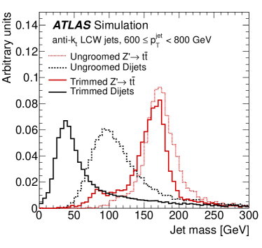
(a) anti-$k_{\rm T}$ $R=1.0$

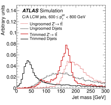
(b) $\mathrm{C/A}$ $R=1.2$

Figure 22: The mass of the leading $p_{\rm T}$ fat jet in simulated ATLAS events before and after applying the trimming procedure with $f_{\rm cut}=5\%$ and $R_{\rm sub}=0.3$. The fat jet $p_{\rm T}$ ranges from $600$ to $800{\mathrm{\ Ge\kern-1.00006ptV}}$ and the jets have been reconstructed using (a) the anti-$k_{\rm T}$ algorithm with $R=1.0$ and (b) the $\mathrm{C/A}$ algorithm with $R=1.2$. Shown are distributions for $Z^{\prime}\rightarrow t\bar{t}$ events with $m_{Z^{\prime}}=1.6{\mathrm{\ Te\kern-1.00006ptV}}$, simulated using PYTHIA and for multijet events from POWHEG+PYTHIA. From [106].

The fat jet mass for the chosen signal and background events is shown in Figure 22. The ungroomed mass of anti-$k_{\rm T}$ jets in signal events is peaked near the top quark mass. Trimming with parameters $f_{\rm cut}=5\%$ and $R_{\rm sub}=0.3$ removes part of the constituents which shifts the distribution to lower masses. The peak position shifts by $5$–$10{\mathrm{\ Ge\kern-1.00006ptV}}$. In some cases, the clusters from the $b$-jet are removed, giving rise to the shoulder at $m_{W}$.

The jet mass is smaller for background because the partons themselves have negligible mass and the jet mass is generated geometrically in quasi-collinear splitting (cf. (10)). The trimming effect is larger for the background jets because for them more soft particles contribute to the mass while the mass of signal jets is dominated by three hard particle jets. The original background distribution is peaked near $100{\mathrm{\ Ge\kern-1.00006ptV}}$ and trimming shifts it down by $60{\mathrm{\ Ge\kern-1.00006ptV}}$. The separation of signal and background is therefore improved by the application of trimming. To select events with top quarks, the trimmed fat jet mass is required to lie in a mass window around the true top quark mass. Other grooming techniques can be used instead of trimming.

For $\mathrm{C/A}$ $R=1.2$ jets, the ungroomed mass distributions are broader and the masses larger on average when compared with the anti-$k_{\rm T}$ $R=1.0$ jets. Trimming yields mass distributions similar to the ones of the trimmed anti-$k_{\rm T}$ jets. The ungroomed $\mathrm{C/A}$ jets therefore contain more soft constituents that lie at large angles to the jet axis. This is what one naively expects from the larger radius parameter but $\mathrm{C/A}$ jets are not cone-like. Figure 23 shows the jet catchment area [105] for anti-$k_{\rm T}$ and $\mathrm{C/A}$ jets for $40<p_{\rm T}<80{\mathrm{\ Ge\kern-1.00006ptV}}$. This area is calculated by including in the jet clustering a large number of ghosts which are distributed according to a fine grid in $(y,\phi)$. The ghosts carry no significant energy such that they do not affect the kinematics of the jet. By looking at the ghosts which end up in the jet, the catchment area of the jet can be determined. The area of anti-$k_{\rm T}$ jets is close to $\pi R^{2}$, with the peak for $R=0.6$ being narrower than the one for $R=0.4$, which is why it is reasonable to assume that the area will scale similarly when going to $R=1.0$. For $\mathrm{C/A}$ $R=1.2$ jets the distribution is much broader and the most probable area is $0.7\times\pi\times 1.2^{2}\approx\pi$, which corresponds to the area of anti-$k_{\rm T}$ $R=1.0$ jets. For approximately equal areas, the irregular shape of a $\mathrm{C/A}$ jet implies that it contains more constituents at large angles to the jet axis which leads to a larger mass. The average area for $\mathrm{C/A}$ jets is also slightly larger because the distribution is asymmetric with a more pronounced large area tail.

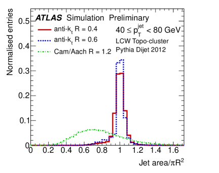
Figure 23: Catchment areas of jets reconstructed with different jet algorithms from the same simulated ATLAS events. The jet $p_{\rm T}$ at the local cluster weighting scale (LCW), i.e., corrected to the level of single pions, is between $40$ and $80{\mathrm{\ Ge\kern-1.00006ptV}}$. From [104].

7.2 $k_{\rm T}$ splitting scales

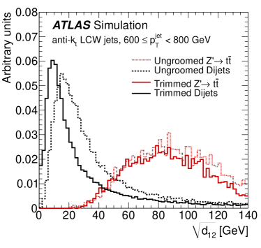
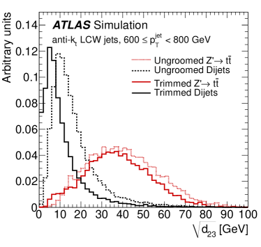
Figure 24: The (a) first and (b) second $k_{\rm T}$ splitting scale of the leading $p_{\rm T}$ anti-$k_{\rm T}$ $R=1.0$ fat jet in simulated ATLAS events before and after applying the trimming procedure with $f_{\rm cut}=5\%$ and $R_{\rm sub}=0.3$. The fat jet $p_{\rm T}$ at the local cluster weighting scale (LCW) ranges from $600$ to $800{\mathrm{\ Ge\kern-1.00006ptV}}$. Shown are distributions for $Z^{\prime}\rightarrow t\bar{t}$ events with $m_{Z^{\prime}}=1.6{\mathrm{\ Te\kern-1.00006ptV}}$, simulated using PYTHIA and for multijet events from POWHEG+PYTHIA. From [106].

Figure 24 shows the first and second $k_{\rm T}$ splitting scales for anti-$k_{\rm T}$ fat jets whose constituents have been reclustered using the $k_{\rm T}$ algorithm. For the top jets, the first scale $\sqrt{d_{12}}$ shows a broad peak near $m_{t}/2$ and $\sqrt{d_{23}}$ peaks at $\approx\!m_{W}/2$. For background jets the values are much lower because the transverse momenta in their mergings are more asymmetric. Trimming affects signal jets only slightly but has a significant impact on the background jets. The distributions for $\mathrm{C/A}$ fat jets are similar. Top quark jets can be selected by requiring, e.g., $\sqrt{d_{12}}>40{\mathrm{\ Ge\kern-1.00006ptV}}$ and $\sqrt{d_{23}}>20{\mathrm{\ Ge\kern-1.00006ptV}}$ for the trimmed jets.

7.3 $N$-subjettiness

$N$-subjettiness is a variable that quantifies to what extend the constituents of a jet align along $N$ subjet axes. The constituents of a jet with radius $R$ are clustered exclusively into $N$ subjets using the $k_{\rm T}$ algorithm. The $N$-subjettiness $\tau_{N}$ is defined as the normalised $p_{\rm T}$-weighted sum of the constituent distances to the nearest subjet axis:

$$\tau_{N}\equiv\frac{1}{d_{0}}\,\sum_{k=1}^{M}\left(p_{{\rm T},k}\times\Delta R^{\rm min}_{k}\right)\,.$$ (20)

The sum is over all $M$ constituents $k$, and $\Delta R^{\rm min}_{k}$ is the distance of $k$ to the nearest subjet axis. The normalisation is given by the variable $d_{0}$ which is the sum of the $p_{\rm T}$ of all constituents multiplied by $R$.

For $N=M$ each constituent represents a subjet and $\tau_{M}=0$. For $N=1$ all constituents are clustered into a single $k_{\rm T}$ jet and in almost all cases $\tau_{1}<1$.

If the internal jet structure follows an $N$-prong pattern, then $\tau_{N}$ is significantly smaller than $\tau_{N-1}$ because the constituents align more closely with the axes of the $N$ subjets. A useful variable to identify hadronic top quark decay is therefore $\tau_{32}\equiv\tau_{3}/\tau_{2}$ while $\tau_{21}\equiv\tau_{2}/\tau_{1}$ is used for 2-prong decays, like that of $Z$ or $W$ bosons.

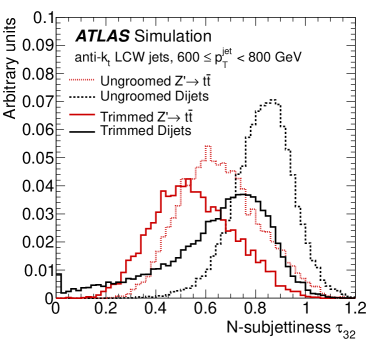
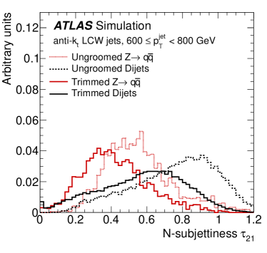
Figure 25: $N$-subjettiness ratios $\tau_{32}$ (a) and $\tau_{21}$ (b) for the leading $p_{\rm T}$ anti-$k_{\rm T}$ $R=1.0$ fat jet in simulated ATLAS events before and after applying the trimming procedure with $f_{\rm cut}=5\%$ and $R_{\rm sub}=0.3$. The fat jet $p_{\rm T}$ at the local cluster weighting scale (LCW) ranges from $600$ to $800{\mathrm{\ Ge\kern-1.00006ptV}}$. Shown are distributions for $Z^{\prime}\rightarrow t\bar{t}$ events with $m_{Z^{\prime}}=1.6{\mathrm{\ Te\kern-1.00006ptV}}$, simulated using PYTHIA and for multijet events from POWHEG+PYTHIA. From [106].

Distributions of $\tau_{32}$ for signal and background fat jets are shown in Figure 25a. Jets with hadronic top quark decay products are better described by three than by two subjets and hence have small average $\tau_{32}$. For background jets the additional subjet does not reduce $\tau_{3}$ much compared to $\tau_{2}$. Trimming affects signal and background jets similarly. A typical cut to enrich top quark decays is $\tau_{32}<0.65$ for trimmed fat jets. Trimmed jets are used for the cut because the $N$-subjettiness of trimmed jets is better described by simulation than that of ungroomed jets, as will be shown in Section 8.4.

Figure 25b shows $\tau_{21}$ but here the signal is given by hadronic SM $Z$ boson decays. These jets are better described by two subjets than the background jets, resulting in a smaller value of $\tau_{21}$. Again, trimming does not help to separate signal and background. The distributions for $\mathrm{C/A}$ fat jets look similar [106] (not shown).

7.4 Top Template Tagger

The Top Template Tagger method [115, 116] compares the energy distribution inside a jet with a template at the parton level. The agreement is quantified in terms of the energy difference between the energies of the three final state partons in $t\rightarrow bqq$ and the energies of the calorimeter clusters in the vicinity of the partons. The method represents a typical energy flow tagger.

The technique has first been applied to measured jets in an ATLAS analysis that searched for $t\bar{t}$ resonances [117], which is discussed in Section 10.2.2. In this analysis, the overlap of a parton configuration with the measured calorimeter cluster energies is given by

$${\rm overlap}=\exp\Biggl{[}-\sum_{\underset{i=1}{\rm parton}}^{3}\frac{1}{2\sigma_{i}^{2}}\Bigl{(}E_{i}-\!\!\underset{<0.2}{\sum_{\Delta R_{\eta}(\mathrm{clus},i)}}\!\!\!E_{\mathrm{clus}}\Bigr{)}^{2}\Biggr{]}\,,$$ (21)

in which $\sigma_{i}\equiv E_{i}/3$ and the minimum cluster $p_{\rm T}$ is $2{\mathrm{\ Ge\kern-1.00006ptV}}$. Clusters are matched to partons if the distance in $(\eta,\phi)$ space $\Delta R_{\eta}\equiv\sqrt{(\Delta\eta)^{2}+(\Delta\phi)^{2}}$ is less than $0.2$, which corresponds to the approximate angular calorimeter resolution. The overall performance of the method has been found to be insensitive to the particular choices of the matching cone size, the normalisation variable $\sigma_{i}$, and the minimum cluster $p_{\rm T}$.

A parton configuration is a specific arrangement of the four-momenta of the quarks. Millions of configurations have to be calculated and stored as templates to cover the full three-body decay phase space to sufficient granularity to allow separation of background. The overlap is calculated for each template according to (21) and the maximum overlap of all templates is called $OV_{3}$.

Figure 26: Normalised distribution of the Top Template Tagger overlap variable $OV_{3}$ for the leading $p_{\rm T}$ anti-$k_{\rm T}$ $R=1.0$ fat jet with $p_{\rm T}>500{\mathrm{\ Ge\kern-1.00006ptV}}$ at the local cluster weighting scale (LCW) in an ATLAS data sample that is dominated by multijet events. Also shown are distributions for simulated events from PYTHIA with multijets and with a hypothetical $Z^{\prime}$ boson of mass $2{\mathrm{\ Te\kern-1.00006ptV}}$ that decays to $t\bar{t}$. From [117].

The distribution of $OV_{3}$ is shown in Figure 26 for the leading $p_{\rm T}$ anti-$k_{\rm T}$ $R=1.0$ fat jet with $p_{\rm T}>500{\mathrm{\ Ge\kern-1.00006ptV}}$ in ATLAS multijet events and in simulated events with a heavy hypothetical $Z^{\prime}$ boson that decays to $t\bar{t}$. The overlap is on average larger for the $Z^{\prime}$ events and a cut $OV_{3}>0.7$ is used to enhance signal over background in the resonance search. The background distribution rises towards large values of $OV_{3}$ because some background jets look top-like by maximising the overlap accidentally. The description of the data is not perfect, especially at high values, and that is the reason why the background in the resonance analysis is not taken from simulation but from data in side-bands.

A second variable used in the tagger to enhance the signal contribution is the fat jet mass which is required to be within $\pm 50{\mathrm{\ Ge\kern-1.00006ptV}}$ of the top quark mass of $172.3{\mathrm{\ Ge\kern-1.00006ptV}}$. The mass is sensitive to pile-up contributions as discussed in Section 7.1. The average mass shift is measured in data as a function of the energy flow away from the jet and a correction is applied [118, 119].

The combination of cuts on $OV_{3}$ and the fat jet mass results in an efficiency of $\approx\!75\%$ for tagging top quarks and a fake rate of $\approx\!10\%$ for tagging fat jets that originate from hard light quarks or gluons. Both cuts are found to be equally important in the background suppression.

7.5 Johns Hopkins Top Tagger

The Johns Hopkins Top Tagger [120] was the first public prong-based top quark tagger. It was adopted with small changes by CMS (cf. Section 7.6). A $\mathrm{C/A}$ fat jet is iteratively declustered with the goal of identifying three or four hard subjets. This is done by searching for the last two mergings of hard protojets.

The last clustering of the fat jet is undone, yielding two protojets. If the $p_{\rm T}$ of each protojet exceeds a fraction $\delta_{p}$ (typically $5\%$ or $10\%$) of the fat jet $p_{\rm T}$ then both protojets are kept and represent the last hard merging. It frequently happens, because $\mathrm{C/A}$ ordering is by angular separation, that a soft protojet (or even a constituent) is combined with a hard protojet in the last step. The hard structure of the fat jet is then represented by the structure of the hard protojet. Therefore, mergings where one of the protojets has $p_{\rm T}<\delta_{p}\times p_{\rm T}^{\rm fat\,jet}$ are skipped and the search for the last hard merging continues by decomposing the hard protojet. This procedure continues until the last hard merging has been found or the two protojets are both soft, too close to each other (specified by a parameter $\delta_{r}$ of the algorithm), or the protojet is a constituent. In the last three cases, the fat jet is considered to be irreducible. The two protojets of the last hard merging are then decomposed following the same procedure. If for one (both) of them a last hard merging is found, the resulting three (four) protojets are taken as the hard subjets of the fat jet.

Kinematic cuts are applied to reject fat jets that do not contain the decay products of a top quark. The invariant mass obtained when combining the subjets should be near the top quark mass, two subjets should give the $W$ boson mass and the reconstructed $W$ boson helicity angle should be consistent with top quark decay. The efficiency for tagging top quarks when using $R=0.8$ fat jets with $1.0<p_{\rm T}<1.1{\mathrm{\ Te\kern-1.00006ptV}}$ is $\approx\!40\%$ and the fake rate for quark and gluon jets is below $2\%$. The inefficiency results from losses due to the subjet finding procedure and the kinematic cuts. A detailed description of the algorithm and of its performance is given in [120].

7.6 CMS Top Tagger

The CMS Top Tagger[121] is based on the Johns Hopkins Top Tagger. Fat jets are built using the $\mathrm{C/A}$ algorithm with $R=0.8$ and three or four subjets are required to be identified using the procedure described in Section 7.5 with $\delta_{p}=5\%$.

The invariant mass is calculated for all pairs of the three leading $p_{\rm T}$ subjets and all of these pairwise masses are required to exceed $50{\mathrm{\ Ge\kern-1.00006ptV}}$. This requirement is motivated by the fact that in more than $60\%$ of all hadronic top quark decays the smallest of these invariant masses is formed by the $W$ boson decay jets.

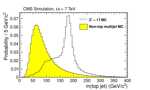
Figure 27: Normalised distributions of the CMS Top Tagger top quark candidate mass in simulated $Z^{\prime}\rightarrow t\bar{t}$ events (MadGraph+PYTHIA) and multijet events (PYTHIA). From [122].

The tagger has first been applied in a search for $t\bar{t}$ resonances [122] which is discussed in Section 10.2.3 and in which the fat jet mass is required to be in the range from $140$ to $250{\mathrm{\ Ge\kern-1.00006ptV}}$. The top quark candidate mass is shown in Figure 27 for simulated $Z^{\prime}\rightarrow t\bar{t}$ events and for multijet events. A clear signal peak near the top quark mass is obtained while the background distribution is smoothly falling for masses larger than $60{\mathrm{\ Ge\kern-1.00006ptV}}$.

7.7 HEPTopTagger

The HEPTopTagger algorithm [5, 19, 123] identifies the hard substructure of a $\mathrm{C/A}$ $R=1.5$ fat jet and tests it for compatibility with the 3-prong pattern of hadronic top quark decay. The tagger has been developed to find mildly boosted top quarks with $p_{\rm T}>200\,{\mathrm{\ Ge\kern-1.00006ptV}}$ in events with an associated production of $t\bar{t}$ pairs with a Higgs boson. The algorithm uses internal parameters that can be changed to optimise the performance. A detailed explanation of the algorithm is given in the appendix of [19] and only a brief summary is given here. The tagger uses three main steps.

First, the hard substructure of the fat jet is identified and soft contributions are removed. This step starts by undoing the last fat jet clustering. If one of the two resulting subjets carries at least $80\%$ of the fat jet mass then the second subjet is discarded because it likely represents a collinearly radiated gluon. This approach is similar to applying a mass drop criterion with $\mu=0.8$ (cf. Section 3.2.1). The remaining subjets are then iteratively decomposed in the same manner until all subjets have a mass below $m_{\rm cut}$ (default value in ATLAS: $50{\mathrm{\ Ge\kern-1.00006ptV}}$). These subjets constitute the hard fat jet substructure and are referred to as substructure objects to distinguish them from the final subjets which are obtained in the third step. Because of the mass cut-off, the substructure objects typically correspond to several particles (or calorimeter cells).

In the second phase, all combinations of three substructure objects (triplets) are tested for compatibility with hadronic top quark decay. Energy contributions from underlying event and pile-up are removed using a filtering procedure that adapts to the distance of the substructure objects: small radius parameter $\mathrm{C/A}$ jets are built from the constituents of the substructure objects using a filter radius parameter $R_{\rm filt}$ that is given by half of the smallest pair-wise distance in the triplet, but at most $R_{\rm filt}^{\rm max}$. Only the $N_{\rm filt}$ largest $p_{\rm T}$ filter jets are kept for further analysis. If there are fewer than $N_{\rm filt}$ filter jets then all are kept. All other constituents in the triplet under consideration are discarded.

In the third HEPTopTagger step, the constituents of the kept filter jets are clustered into three top quark subjets using the exclusive $\mathrm{C/A}$ algorithm. Under the hypothesis that these subjets correspond to the three products from $t\to bqq$ decay, kinematic cuts are applied on these subjets to reject non-top background. The kinematic constraints are the $W$ boson mass and the Lorentz structure of the $t\to bW$ decay (helicity angle).

The helicity angle $\theta^{*}$ is determined in the rest frame of the $W$ boson as the angle between the top quark momentum and the momentum of one of the $W$ boson decay products (which are back-to-back). The distribution of the cosine of this angle is asymmetric, see for example [124]. For background the distribution is more uniform and a typical cut to enhance the top quark signal is $\cos\theta^{*}<0.6$. Experimentally, the boost to the $W$ boson rest frame is associated with large uncertainties from jet reconstruction which reduce the effectiveness of a direct cut on the reconstructed angle. Instead, the kinematic constraints are formulated in terms of ratios of invariant subjet masses.

With $p_{i}$ ($i=1,2,3$) denoting the four-momenta of the decay quarks in $t\to bqq$, the square of the top quark mass is given by

$$m_{t}^{2}=m_{123}^{2}=(p_{1}+p_{2}+p_{3})^{2} = (p_{1}+p_{2})^{2}+2(p_{1}+p_{2})\cdot p_{3}+m_{3}^{2}$$ (22)

$$= m_{1}^{2}+m_{2}^{2}+m_{3}^{2}+2p_{1}\cdot p_{2}+2p_{1}\cdot p_{3}+2p_{2}\cdot p_{3}\,.$$ (23)

In the limit of negligible subjet masses ($m_{i}^{2}=0$), the equation simplifies to

$$m_{123}^{2} = (p_{1}+p_{2})^{2}+(p_{1}+p_{3})^{2}+(p_{2}+p_{3})^{2}$$ (24)

$$= m_{12}^{2}+m_{13}^{2}+m_{23}^{2}\,.$$ (25)

This is the equation of a sphere with radius $m_{123}=m_{t}$. In the limit $m_{i}^{2}=0$, the kinematics of the decay $t\to bqq$ is fully specified for each point on the surface of this sphere. The kinematics is therefore described by the two angles of spherical coordinates,

$$\cos\theta = m_{23}/m_{123}\,,$$ (26)

$$\phi = \arctan(m_{13}/m_{12})\,.$$ (27)

In the HEPTopTagger, the final three exclusively clustered subjets are identified with the top quark decay products, such that $p_{1}$ denotes the four-momentum of the leading $p_{\rm T}$ subjet, $p_{2}$ that of the subleading $p_{\rm T}$ subjet, and $p_{3}$ that of the sub-subleading $p_{\rm T}$ subjet.

Figure 28 shows how the subjet kinematics is distributed on the surface of the sphere given by (25) in terms of the coordinates $\cos\theta$ and $\phi$ as defined in (26) and (27) for fat jets in different event samples. Shown are the distributions for signal events (SM $t\bar{t}$ production) and background events ($W\!$+jets and multijets (QCD)). The signal distribution resembles the shape of the letter A. As written on the plots in the figure, the arms of the letter A can be identified with the relations

$$m_{23} \approx m_{W}\quad{\rm(horizontal\leavevmode\nobreak\ arm)},$$ (28)

$$m_{12} \approx m_{W}\quad{\rm(right\leavevmode\nobreak\ arm)},$$ (29)

$$m_{13} \approx m_{W}\quad{\rm(left\leavevmode\nobreak\ arm)},$$ (30)

in which $m_{W}=80.4{\mathrm{\ Ge\kern-1.00006ptV}}$ denotes the $W$ boson mass. Most of the background is located below $m_{23}/m_{123}=0.35$. Kinematic cuts are now defined that reject most of the background while retaining the signal.

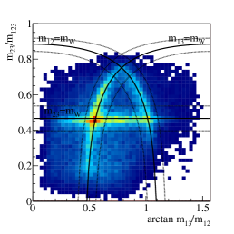
(a) $t\bar{t}$

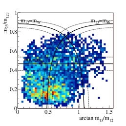
(b) $W\!$+jets

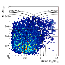
(c) Multijets (QCD)

Figure 28: Distributions of kinematics of the final three subjets used in the HEPTopTagger for (a) SM $t\bar{t}$ production, (b) $W\!$+jets events, and (c) multijet events. Shown is the surface of the sphere defined by $m_{123}^{2}=m_{12}^{2}+m_{13}^{2}+m_{23}^{2}.$ The quantity $m_{123}$ is the invariant mass of all three subjets. The quantities $m_{ij}$ are invariant masses of two of the subjets which are ordered in $p_{\rm T}$ such that $p_{{\rm T},1}>p_{{\rm T},2}>p_{{\rm T},3}$. From [19].

The relations in (28)–(30) are formulated in terms of a $W$ boson mass window which is specified by $R_{\mp}=(1\mp f_{\rm W})\,m_{W}/m_{t}$ in which the width is given by $f_{\rm W}$ which has a default value of $15\%$ and $m_{t}=172.3{\mathrm{\ Ge\kern-1.00006ptV}}$ (this value stems from a previous best global value of the measured top quark mass):

$$m_{23}\approx m_{W}: R_{-}<\frac{m_{23}}{m_{123}}<R_{+}$$ (31)

$$m_{12}\approx m_{W}: R_{-}^{2}\left(1+\left(\frac{m_{13}}{m_{12}}\right)^{2}\right)<1-\left(\frac{m_{23}}{m_{123}}\right)^{2}<R_{+}^{2}\left(1+\left(\frac{m_{13}}{m_{12}}\right)^{2}\right)$$ (32)

$$m_{13}\approx m_{W}: R_{-}^{2}\left(1+\left(\frac{m_{12}}{m_{13}}\right)^{2}\right)<1-\left(\frac{m_{23}}{m_{123}}\right)^{2}<R_{+}^{2}\left(1+\left(\frac{m_{12}}{m_{13}}\right)^{2}\right)$$ (33)

With the relations $m_{ij}\approx m_{W}$ used as short-hand notations for the mass windows specified in (31)–(33), the kinematic selection cuts for the HEPTopTagger subjets are given by

$$\left(m_{23}\approx m_{W}\quad{\rm and}\quad 0.2<\arctan(m_{13}/m_{12})<1.3\right)$$ (34)

$${\rm or} \left(m_{12}\approx m_{W}\quad{\rm and}\quad m_{23}/m_{123}>0.35\right)$$ (35)

$${\rm or} \left(m_{13}\approx m_{W}\quad{\rm and}\quad m_{23}/m_{123}>0.35\right)\,.$$ (36)

The HEPTopTagger therefore requires one of the three possible subjet pairs to reconstruct the $W$ boson mass but it does not explicitly reconstruct the $W$ boson or identify the $b$-quark jet.

The top quark candidate four-momentum vector is given by the sum of the vectors of the $N_{\rm filt}$ largest $p_{\rm T}$ filter jets. The top quark candidate mass has to lie in a window around the measured top quark mass, usually $140$–$200{\mathrm{\ Ge\kern-1.00006ptV}}$. If all criteria are met, the fat jet is considered to be tagged. If several top quark candidates are found, the one with mass closest to $172.3{\mathrm{\ Ge\kern-1.00006ptV}}$ is used.

The parameter settings used in this text are summarised in Table 1. The parameters listed in the ‘default’ column gave the best expected significance in a search for $t\bar{t}$ resonances in the hadronic decay channel [117] which is discussed in Section 10.2.1.

parameter	default	default-30	tight	loose
$m_{\rm cut}$ (GeV)	$50$	$30$	$30$	$70$
$R_{\rm filt}^{\rm max}$	$0.3$		$0.2$	$0.5$
$N_{\rm filt}$	$5$		$4$	$7$
$f_{\rm W}$	$15\%$		$10\%$	$20\%$

Table 1: HEPTopTagger parameter settings.

8 Measurements of Jet Structure

This section presents measurements of jet substructure variable distributions at the detector level and distributions corrected to the level of stable particles (lifetime longer than 10 ps). The impact of pile-up energy is evaluated for ungroomed and groomed jets.

8.1 Data samples

The studies presented in this section have been performed using data collected with the ATLAS detector in $pp$ collisions in 2010 [54], 2011 [106], and 2012 [102]. The increased luminosity in each year allowed the study of different event topologies.

In 2010, the integrated luminosity was $35(1)\leavevmode\nobreak\ {\rm pb}^{-1}$. This dataset is used to study the structure of non-top fat jets that occur in dijet or multijet production because no significant number of boosted top quarks were produced. An advantage of this dataset is that pile-up was very limited: approximately $22\%$ of the events had only one reconstructed primary vertex (with at least five tracks). This allows to study fat jets in the absence of pile-up and how the structure changes in the presence of a few additional vertices. Fat jets are reconstructed using the $\mathrm{C/A}$ algorithm with $R=1.2$ and the anti-$k_{\rm T}$ algorithm with $R=1.0$. To show the effect of grooming, mass drop filtering (cf. Sections 3.2.1 and 3.4) is applied to the $\mathrm{C/A}$ jets. The mass drop criterion with $\mu=0.67$ and $v_{\rm cut}=0.09$ is used to identify two subjets which must be separated by $\Delta R_{12}\geq 0.3$. Compared to the original jet, a jet that satisfies this MD criterion exhibits a 2-prong structure like that expected from hadronic heavy particle decay ($W$, $Z$, or Higgs bosons): two hard subjets (each with $p_{\rm T}>15\%$ of the sum of the two subjet transverse momenta) and a significant mass increase when the two subjets are combined. The fraction of jets in this data sample that contain decay products of heavy particles is negligible. A jet that survives the splitting/filtering criteria is a background jet that displays the 2-prong pattern by accident.

Filtering is applied to the jets that pass the MD criterion to reject pile-up and underlying event activity: the separation $\Delta R_{12}$ of the two subjets identified by the MD procedure is used to determine the filter radius $R_{\rm filt}=\min(0.3,\Delta R_{12}/2)$ and the three leading $p_{\rm T}$ filter jets (or all if fewer than three are found) when clustering all constituents of the original fat jet are combined to obtain a split/filtered fat jet. The data are corrected for detector effects using matrix-based unfolding with simulated events from PYTHIA. SHERPA events are used to estimate systematic uncertainties.

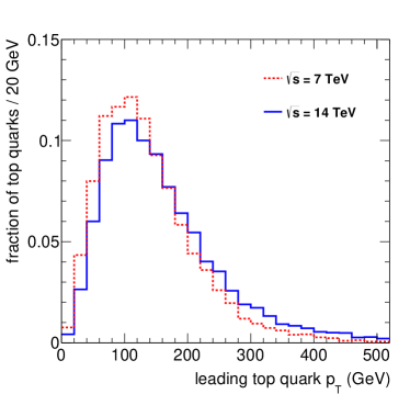
Figure 29: Normalised distributions of the leading top quark $p_{\rm T}$ in $t\bar{t}$ events simulated with PYTHIA 8 for two LHC centre-of-mass energies.

The 2011 data correspond to $4.7(1)\leavevmode\nobreak\ {\rm fb}^{-1}$. In this dataset, a significant number of top quarks with $p_{\rm T}>200{\mathrm{\ Ge\kern-1.00006ptV}}$ are present. The $p_{\rm T}$ spectrum of the leading $p_{\rm T}$ top quark in SM $t\bar{t}$ events generated with PYTHIA 8 is shown in Figure 29. The fraction of leading $p_{\rm T}$ top quarks with $p_{\rm T}>200{\mathrm{\ Ge\kern-1.00006ptV}}$ is $18\%$ for $\sqrt{s}=7{\mathrm{\ Te\kern-1.00006ptV}}$ and $27\%$ for $\sqrt{s}=14{\mathrm{\ Te\kern-1.00006ptV}}$. Using this fraction in combination with the approximate NNLO cross section for $t\bar{t}$ production of 167 pb (cf. Section 2.1), the number of $t\bar{t}$ events with top quark $p_{\rm T}>200{\mathrm{\ Ge\kern-1.00006ptV}}$ in the 2011 data sample is predicted to be approximately $142,\!000$. Events with $t\bar{t}$ pairs from 2011 will be used in the HEPTopTagger performance studies in Section 9.1. For the substructure variables discussed in the present section, multijet events from 2011 and $t\bar{t}$ events from 2012 are used. The multijet events differ from those in the 2010 data by the much larger pile-up energy (average $\mu=9.1$). The main goal is therefore the study of fat jets (anti-$k_{\rm T}$ $R=1.0$) with $p_{\rm T}>350{\mathrm{\ Ge\kern-1.00006ptV}}$, both ungroomed (i.e., including the pile-up energy) and trimmed (using the parameters $f_{\rm cut}=5\%$ and $R_{\rm sub}=0.3$ introduced in Section 3.4).

From the 2012 data sample, corresponding to $20.3(6)\leavevmode\nobreak\ {\rm fb}^{-1}$ at $\sqrt{s}=8{\mathrm{\ Te\kern-1.00006ptV}}$, SM $t\bar{t}$ events, in which one $W$ boson decays to a neutrino and a muon, are selected as follows. Events must contain exactly one muon with $p_{\rm T}>25{\mathrm{\ Ge\kern-1.00006ptV}}$ and $|\eta|<2.5$ and have missing transverse momentum $\mbox{$/{\!\!\!\!E_{\rm T}}$}>20{\mathrm{\ Ge\kern-1.00006ptV}}$. The scalar sum of $/{\!\!\!\!E_{\rm T}}$ and the transverse mass $m^{W}_{\rm T}$ of the leptonic $W$ boson candidate must be larger than $60{\mathrm{\ Ge\kern-1.00006ptV}}$, where $m^{W}_{\rm T}=\sqrt{2\,p_{{\rm T},\mu}\,\mbox{$/{\!\!\!\!E_{\rm T}}$}\,(1-\cos\Delta\phi)}$ in which $\Delta\phi$ is the azimuthal angle between the muon-$p_{\rm T}$ and $/{\!\!\!\!E_{\rm T}}$ vectors. To reduce contamination from $W\!$+jets events, each event must contain at least one $b$-tagged anti-$k_{\rm T}$ $R=0.4$ jet with $p_{\rm T}>20{\mathrm{\ Ge\kern-1.00006ptV}}$ and $|\eta|<2.5$ within $\Delta R_{\eta}=1.5$ of the muon. Substructure variable distributions will be shown in the following for anti-$k_{\rm T}$ $R=1.0$ jets which have been trimmed like the 2011 jets. The $t\bar{t}$ simulation is divided into two categories, contained and non-contained. A hadronically decaying top quark is said to be contained if all decay quarks are separated by less than $\Delta R_{\eta}=1.0$ from the top quark flight direction.

8.2 Jet mass

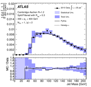
Figure 30: Unfolded normalised distribution of the mass of $\mathrm{C/A}$ $R=1.2$ jets with $300<p_{\rm T}<400{\mathrm{\ Ge\kern-1.00006ptV}}$ a) before and b) after splitting and filtering in an inclusive jet sample without pile-up (number of primary vertices $N_{\rm PV}=1$). From [54].

Figure 30 shows the normalised particle level measurement of the mass of $\mathrm{C/A}$ $R=1.2$ jets before (left panel) and after splitting and filtering (right panel) for $300<p_{\rm T}<400{\mathrm{\ Ge\kern-1.00006ptV}}$ in events with only one primary vertex, i.e., without pile-up. The mass is peaked between $70$ and $80{\mathrm{\ Ge\kern-1.00006ptV}}$ for the original jets and between $90$ and $100{\mathrm{\ Ge\kern-1.00006ptV}}$ for the split/filtered jets. The higher mass is explained by the requirement $\Delta R_{12}\geq 0.3$ used in the splitting. The PYTHIA prediction for the original jet mass spectrum (the one before splitting and filtering) tends to be too soft, with the ratio to the measured distribution varying between $1.2$ and $0.8$. Although this is within the measurement uncertainties, a clear trend is visible. The HERWIG++ prediction is too hard, within $+30\%$ and $-40\%$ of the data. The level of description by the simulation is similar for jet $p_{\rm T}$ between $200$ and $600{\mathrm{\ Ge\kern-1.00006ptV}}$ and for anti-$k_{\rm T}$ $R=1.0$ jets (not shown). The shape of the mass distribution of split/filtered jets in Figure 30b is well described, indicating that the problem lies in the simulation of soft hadrons. Potential candidates for improvement are the underlying event models and their tunes, and the fragmentation models.

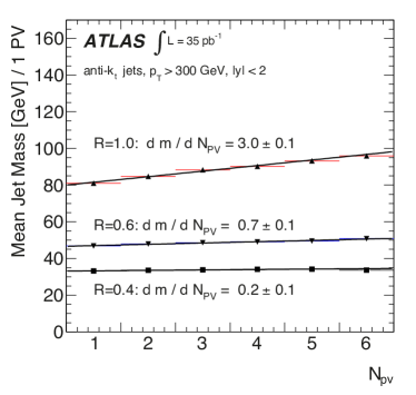
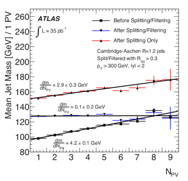
Figure 31: The average detector level mass of jets with $p_{\rm T}>300{\mathrm{\ Ge\kern-1.00006ptV}}$ as a function of the number of reconstructed primary vertices in the event. Shown are a) anti-$k_{\rm T}$ jets with different radius parameters $R$ and b) C/A $R=1.2$ jets before grooming, after the mass drop criterion (splitting), and after mass drop filtering (splitting/filtering). From [54].

The average detector level jet mass is shown in Figure 31a for anti-$k_{\rm T}$ jets with different radius parameters as a function of the number $N_{\rm PV}$ of reconstructed primary vertices in the event. The number $N_{\rm PV}$ is a measure of the number of inelastic $pp$ interactions in the event. For $R=0.4$, the jet mass is $\approx\!35{\mathrm{\ Ge\kern-1.00006ptV}}$ and does not depend on $N_{\rm PV}$. For $R=0.6$ ($1.0$), the mass is $55{\mathrm{\ Ge\kern-1.00006ptV}}$ ($80{\mathrm{\ Ge\kern-1.00006ptV}}$) without pile-up and increases by $0.7(1){\mathrm{\ Ge\kern-1.00006ptV}}$ ($3.0(1){\mathrm{\ Ge\kern-1.00006ptV}}$) per primary vertex. As described in [54], the jet mass pile-up dependence $d\langle m\rangle/dN_{\rm PV}$ is approximately proportional to $R^{3}$: the ratios of the fitted slopes $s_{R}$ are

$$s_{1.0}/s_{0.6} =4.3\pm 0.5 ((1.0/0.6)^{3} =4.6),$$

$$s_{1.0}/s_{0.4} =13\pm 3 ((1.0/0.4)^{3} =15.6),$$

$$s_{0.6}/s_{0.4} =3.0\pm 0.8 ((0.6/0.4)^{3} =3.4)\,,$$

in good agreement with $R^{3}$ scaling. This scaling is explained by two factors. First, the jet area of anti-$k_{\rm T}$ jets is $\approx\!\pi R^{2}$ (cf. Section 7.1 and Figure 23). The amount of pile-up energy in a jet is proportional to the jet area because the pile-up energy is approximately equally distributed in $(y,\phi)$. Another power of $R$ results from the separation of the constituents (cf. (10)).

The pile-up dependence of the $\mathrm{C/A}$ $R=1.2$ jet mass is shown in Figure 31b. The mass is $100{\mathrm{\ Ge\kern-1.00006ptV}}$ and rises with $4.2(1){\mathrm{\ Ge\kern-1.00006ptV}}$ per vertex. The jet mass is also shown for the jets that satisfy the mass drop criterion before filtering (labelled in the figure as after splitting only). These jets have a larger mass ($150{\mathrm{\ Ge\kern-1.00006ptV}}$ at $N_{\rm PV}=1$) because the $\Delta R_{12}\geq 0.3$ cut enhances configurations with a geometrically induced higher mass (cf. (10)). The dependence on the number of vertices is reduced for these jets, but still significant at $2.9(3){\mathrm{\ Ge\kern-1.00006ptV}}$ per vertex. Efficient pile-up removal is achieved in the filtering step: after applying filtering to the split jets (label after splitting/filtering), the slope is consistent with zero. The mass of the split/filtered jets is reduced ($\approx\!130{\mathrm{\ Ge\kern-1.00006ptV}}$) because only the three leading $p_{\rm T}$ filter jets are used.

Figure 32: Detector level distributions of the mass of anti-$k_{\rm T}$ $R=1.0$ jets with $600<p_{\rm T}<800{\mathrm{\ Ge\kern-1.00006ptV}}$ in multijet events with an average pile-up $\mu$ of $9.1$. a) ungroomed jets and b) trimmed jets using $f_{\rm cut}=5\%$ and $R_{\rm sub}=0.3$. From [106].

Detector level distributions of the jet mass are shown Figure 32 for jets with $600<p_{\rm T}<800{\mathrm{\ Ge\kern-1.00006ptV}}$ in multijet events with an average pile-up $\mu$ of 9.1 (2011 data). Before grooming, the jet mass is peaked at $100$–$120{\mathrm{\ Ge\kern-1.00006ptV}}$ and the description by the Monte Carlo generators is within $\pm 10\%$ for the bulk of the distribution. The shift of the peak position with respect to Figure 30 is in part due to the larger jet $p_{\rm T}$. In Figure 32, HERWIG++ uses a refined UE model (colour reconnection model) [125] with parameters tuned to LHC data (tune UE7-2). The description of the jet mass by HERWIG++ is improved by this model compared to Figure 30 where the default UE model was used. Also the description by PYTHIA is improved, through the use of the parameter set AUET2B [76, 75] which is tuned to LHC data and results in a better prediction than the AMBT1 set [65] used in Figure 30 which was tuned to $e^{+}e^{-}$ and Tevatron data. After trimming, the peak is at $20$–$40{\mathrm{\ Ge\kern-1.00006ptV}}$, with the Monte Carlo distributions within $\pm 20\%$ of the data points up to $250{\mathrm{\ Ge\kern-1.00006ptV}}$. The fact that the ungroomed and the trimmed jet masses are well described by the simulation, where trimming reduces the mass by $\approx\!80{\mathrm{\ Ge\kern-1.00006ptV}}$, demonstrates that pile-up contributions to jets as well their removal is well modelled in the simulation.

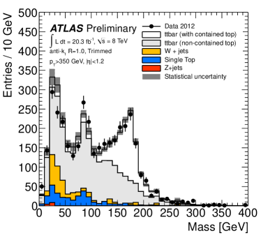
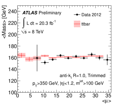
Figure 33: a) Detector level distributions of the mass of trimmed anti-$k_{\rm T}$ $R=1.0$ jets ($f_{\rm cut}=5\%$, $R_{\rm sub}=0.3$) with $p_{\rm T}>350{\mathrm{\ Ge\kern-1.00006ptV}}$ in a selection of semileptonic $t\bar{t}$ decays. Contained refers to hadronically-decaying top quarks for which all three decay quarks are separated by less than $\Delta R_{\eta}=1.0$ from the top quark flight direction. The shaded band represents the statistical simulation uncertainty. b) The average of the distribution of masses larger than $100{\mathrm{\ Ge\kern-1.00006ptV}}$ as a function of the average number of inelastic $pp$ collisions per bunch crossing. The $t\bar{t}$ simulation is obtained from POWHEG with PYTHIA for the parton shower and hadronisation. From [102].

Figure 33a shows the mass distribution for trimmed anti-$k_{\rm T}$ $R=1.0$ fat jets in the event sample obtained with the $t\bar{t}$ selection. The peak at the top quark mass results from hadronically decaying top quarks for which all decay products are captured in the fat jet. The peak at the $W$ boson mass represents the cases in which the $b$-jet is not part of the fat jet. The average mass above $100{\mathrm{\ Ge\kern-1.00006ptV}}$ is shown in Figure 33b as a function of $\mu$. Within the statistical uncertainty of $\approx\!5{\mathrm{\ Ge\kern-1.00006ptV}}$, no pile-up dependence is present. Figure 34 shows the jet mass distribution for different subjet multiplicities. The subjets are reconstructed with the $k_{\rm T}$ algorithm using $R=0.3$ and correspond to the subjets that remain after trimming and have $p_{\rm T}>17.5{\mathrm{\ Ge\kern-1.00006ptV}}=5\%\times 350{\mathrm{\ Ge\kern-1.00006ptV}}$. All distributions are well described by the simulation as is the integrated distribution in Figure 33a. The prediction for $t\bar{t}$ production is obtained from POWHEG with PYTHIA for the parton shower and hadronisation. For exactly one subjet, the fat jet mass peaks at $20$–$30{\mathrm{\ Ge\kern-1.00006ptV}}$ and the fat jet results from hadronic top quark decays with more than one decay jet not captured, background from $W\!$+jets events, or production of single top quarks. With two subjets, the distribution peaks at the $W$ boson mass, indicating that the subjets correspond to the two $W$ boson decay jets. A shoulder towards higher masses is also visible, resulting from $t\to bqq$ decays in which the subjets correspond to one $W$ boson decay jet and the $b$-jet, which has on average larger $p_{\rm T}$. A $W$ boson peak is also visible for events with single top quarks, which therefore seem to contain a hadronically decaying $W$ boson while still satisfying the requirements for an isolated muon and significant $/{\!\!\!\!E_{\rm T}}$. Fat jets with three subjets have a mass that peaks near the top quark mass and result mostly from SM $t\bar{t}$ events in which all top quark decay jets are contained in the fat jet. For four or more subjets, the high mass tail is more pronounced but is still described by $t\bar{t}$ production, indicating that energy from underlying event and/or pile-up is picked up. These studies suggest that the mass of trimmed anti-$k_{\rm T}$ $R=1.0$ jets with exactly three subjets is well suited for the identification of hadronically decaying top quarks.

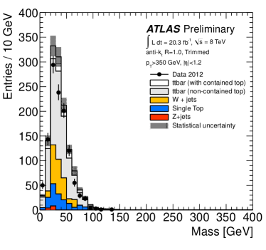
(a) $N_{\rm subjets}=1$

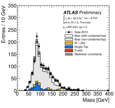
(b) $N_{\rm subjets}=2$

(c) $N_{\rm subjets}=3$

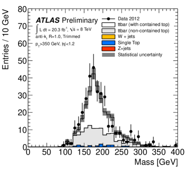
(d) $N_{\rm subjets}\geq 4$

Figure 34: Detector level distributions of the mass of trimmed anti-$k_{\rm T}$ $R=1.0$ jets ($f_{\rm cut}=5\%$, $R_{\rm sub}=0.3$) with $p_{\rm T}>350{\mathrm{\ Ge\kern-1.00006ptV}}$ in a selection of semileptonic $t\bar{t}$ decays for different $k_{\rm T}$ $R=0.3$ subjet multiplicities. Contained refers to hadronically-decaying top quarks for which all three decay quarks are separated by less than $\Delta R_{\eta}=1.0$ from the top quark flight direction. The shaded band represents the statistical simulation uncertainty. The $t\bar{t}$ simulation is obtained from POWHEG+PYTHIA. From [102].

8.3 $k_{\rm T}$ splitting scales

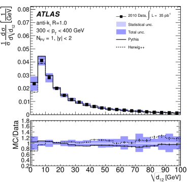
(a) $\sqrt{d_{12}}$

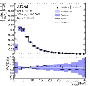
(b) $\sqrt{d_{23}}$

Figure 35: Unfolded normalised distributions of $k_{\rm T}$ splitting scales of anti-$k_{\rm T}$ $R=1.0$ jets with $300<p_{\rm T}<400{\mathrm{\ Ge\kern-1.00006ptV}}$ in an inclusive jet sample without pile-up. From [54].

Normalised distributions of the $k_{\rm T}$ splitting scales $\sqrt{d_{12}}$ and $\sqrt{d_{23}}$ are shown in Figure 35 for jets in multijet events without pile-up overlay energy. The distributions peak in the ranges $5$–$10{\mathrm{\ Ge\kern-1.00006ptV}}$ and $2.5$–$7.5{\mathrm{\ Ge\kern-1.00006ptV}}$, respectively. The uncertainties from unfolding (related mainly to the uncertainty with which the detector jet energy scale and resolution can be simulated) are $\pm 20\%$ in the ranges $5$–$70{\mathrm{\ Ge\kern-1.00006ptV}}$ and $2.5$–$25{\mathrm{\ Ge\kern-1.00006ptV}}$, respectively, which contain the bulk of the data. The predicted distributions describe the data within these uncertainties. Trends are however visible, with the HERWIG++ spectrum being too hard and the one by PYTHIA too soft.

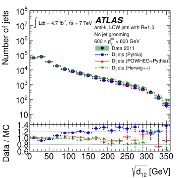
(a) $\sqrt{d_{12}}$

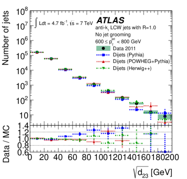
(b) $\sqrt{d_{23}}$

Figure 36: Detector level distributions of $k_{\rm T}$ splitting scales of anti-$k_{\rm T}$ $R=1.0$ jets with $600<p_{\rm T}<800{\mathrm{\ Ge\kern-1.00006ptV}}$ in multijet events with an average pile-up $\mu$ of $9.1$. From [106].

Detector level distributions of the splitting scales are shown in Figure 36 for jets in multijet events with an average pile-up $\mu$ of 9.1. Compared to the no-pile-up case in Figure 35, the horizontal axis now extends to much larger values of the scales and a logarithmic vertical axis is chosen to highlight the tails of the distributions. For $\sqrt{d_{12}}<100{\mathrm{\ Ge\kern-1.00006ptV}}$ and $\sqrt{d_{23}}<40{\mathrm{\ Ge\kern-1.00006ptV}}$, the quality of the descriptions is similar to the no-pile-up case and describes the data within $10$–$20\%$. A typical cut for top quark identification is $\sqrt{d_{12}}>40{\mathrm{\ Ge\kern-1.00006ptV}}$ and the prediction at this value is within $10\%$ of the data. In the tails, POWHEG and HERWIG++ give a better prediction than PYTHIA. The PYTHIA spectra are too soft with the relative difference to the data points being $\approx\!30\%$ for $\sqrt{d_{12}}>160{\mathrm{\ Ge\kern-1.00006ptV}}$ and $\sqrt{d_{23}}>80{\mathrm{\ Ge\kern-1.00006ptV}}$. The HERWIG++ spectrum tends to be too hard for $\sqrt{d_{12}}>200{\mathrm{\ Ge\kern-1.00006ptV}}$. Grooming has little impact on the splitting scales and the quality of the simulation is similar for trimmed jets [106] (not shown).

(a) $\sqrt{d_{12}}$

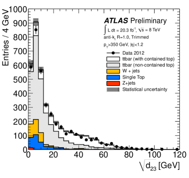
(b) $\sqrt{d_{23}}$

Figure 37: Detector level distributions of the $k_{\rm T}$ splitting scales for trimmed anti-$k_{\rm T}$ $R=1.0$ jets ($f_{\rm cut}=5\%$, $R_{\rm sub}=0.3$) with $p_{\rm T}>350{\mathrm{\ Ge\kern-1.00006ptV}}$ in a selection of semileptonic $t\bar{t}$ decays. Contained refers to hadronically-decaying top quarks for which all three decay quarks are separated by less than $\Delta R_{\eta}=1.0$ from the top quark flight direction. The shaded band represents the statistical simulation uncertainty. The $t\bar{t}$ simulation is obtained from POWHEG+PYTHIA. From [102].

The distributions of the splitting scales for jets in the $t\bar{t}$ event selection are shown in Figure 37. They are well described by the simulation. For contained top quarks, the $\sqrt{d_{12}}$ ($\sqrt{d_{23}}$) distribution peaks at approximately $80$–$90{\mathrm{\ Ge\kern-1.00006ptV}}$ ($35$–$40{\mathrm{\ Ge\kern-1.00006ptV}}$) as expected. The majority of top quarks is however not contained because the radius parameter of $R=1.0$ is not large enough to capture all decay products of top quarks with $p_{\rm T}>350{\mathrm{\ Ge\kern-1.00006ptV}}$ (cf. Figure 4). The splitting scales for non-contained top quarks are naturally smaller. Also these cases are well described.

8.4 $N$-subjettiness

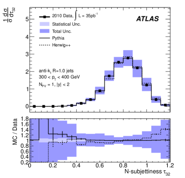
(a) $\tau_{32}$

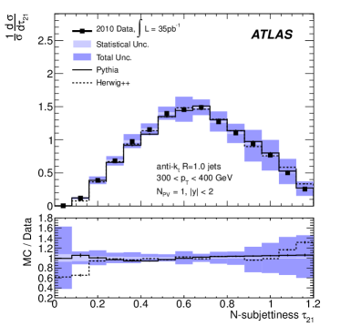
(b) $\tau_{21}$

Figure 38: Unfolded normalised distributions of $N$-subjettiness ratios for anti-$k_{\rm T}$ $R=1.0$ jets with $300<p_{\rm T}<400{\mathrm{\ Ge\kern-1.00006ptV}}$ in an inclusive jet sample without pile-up. From [54].

Normalised distributions of the measured $N$-subjettiness ratios $\tau_{32}$ and $\tau_{21}$ at the particle level are shown in Figure 38 for jets in multijet events without pile-up overlay energy. The most probable values are $\approx\!0.85$ for $\tau_{32}$ and $\approx\!0.7$ for $\tau_{21}$. The bulk of each distribution is described by simulations within the measurement uncertainties, which amount to $\pm 20\%$ and $\pm 10\%$, respectively.

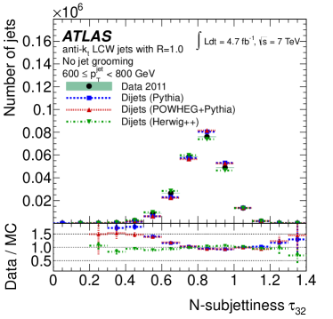
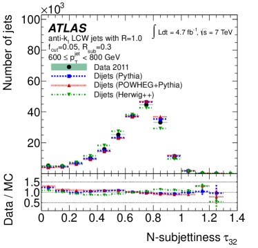
Figure 39: Detector level distributions of the $N$-subjettiness ratio $\tau_{32}$ for anti-$k_{\rm T}$ $R=1.0$ jets with $600<p_{\rm T}<800{\mathrm{\ Ge\kern-1.00006ptV}}$ in multijet events with an average pile-up $\mu$ of $9.1$ a) before trimming and b) after trimming with $f_{\rm cut}=5\%$ and $R_{\rm sub}=0.3$. From [106].

Detector level distributions of the $N$-subjettiness ratio $\tau_{32}$ are shown in Figure 39 for jets in multijet events with an average pile-up $\mu$ of 9.1. The distribution for ungroomed jets peaks at $0.8$–$0.9$ (panel a) like in the no-pile-up case. HERWIG++ (with the UE model parameters tuned to LHC data) gives the best description while PYTHIA and POWHEG+PYTHIA underestimate the tail for $\tau_{32}<0.7$. Trimming shifts the distributions by $0.1$ to lower values and increases the tail (panel b). Trimming therefore makes the non-top jets more top-like. This has already been observed in simulation in Section 7.3. A benefit of trimming is, however, that it improves the description of the distribution by simulation: all generators yield a description within $10\%$ of the data.

A similar observation is made for $\tau_{21}$ which is shown in Figure 40. Also here, HERWIG++ gives the best description before trimming. After trimming, the HERWIG++ distribution is shifted to lower values, although still within $\pm 20\%$ of the data points. The PYTHIA prediction underestimates the data in the tail ($\tau_{21}<0.6$) by $30\%$ or more and is shifted towards high values. Trimming reduces the discrepancy in the tail to $20\%$ but the distribution is still shifted. This shift is also seen for POWHEG with trimming having little effect.

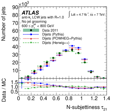
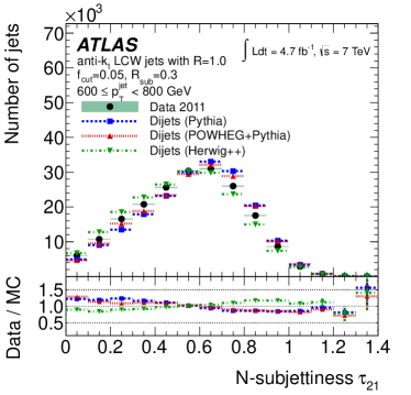
Figure 40: Detector level distributions of the $N$-subjettiness ratio $\tau_{21}$ for anti-$k_{\rm T}$ $R=1.0$ jets with $600<p_{\rm T}<800{\mathrm{\ Ge\kern-1.00006ptV}}$ in multijet events with an average pile-up $\mu$ of $9.1$ a) before trimming and b) after trimming with $f_{\rm cut}=5\%$ and $R_{\rm sub}=0.3$. From [106].

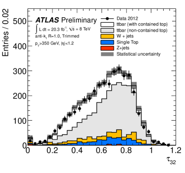
(a) $\tau_{32}$

(b) $\tau_{21}$

Figure 41: Detector level distributions of $N$-subjettiness ratios for trimmed anti-$k_{\rm T}$ $R=1.0$ jets ($f_{\rm cut}=5\%$, $R_{\rm sub}=0.3$) with $p_{\rm T}>350{\mathrm{\ Ge\kern-1.00006ptV}}$ in a selection of semileptonic $t\bar{t}$ decays. Contained refers to hadronically-decaying top quarks for which all three decay quarks are separated by less than $\Delta R_{\eta}=1.0$ from the top quark flight direction. The shaded band represents the statistical simulation uncertainty. The $t\bar{t}$ simulation is obtained from POWHEG+PYTHIA. From [102].

The $N$-subjettiness ratios $\tau_{32}$ and $\tau_{21}$ are shown in Figure 41 for fat jets in the $t\bar{t}$ event selection. The distributions are well described by the simulation. Fat jets containing all top quark decay jets have the smallest $\tau_{32}$. This is the expected behaviour because most of the containing fat jets have three or four subjets while the other fat jets have one or two (cf. Figure 34). The 3-prong or 4-prong structure of the fully-containing fat jets leads to reduced $\tau_{3}$ with respect to $\tau_{2}$, and therefore a small value of $\tau_{32}=\tau_{3}/\tau_{2}$. Similarly, fat jets with only two subjets are expected to have the smallest $\tau_{21}$. Figure 41b is compatible with this expectation: the non-containing fat jet contribution at low values of $\tau_{21}$ presumably originates from fat jets with two subjets while that at larger values stems from fat jets with only one subjet.

8.5 Summary of measurements of substructure variables

Jet grooming is a powerful tool to remove the pile-up dependence of substructure variables as was shown for the jet mass. Similar pile-up stability is obtained for the other variables [106] (not shown). The leading order plus parton shower generators HERWIG++ and PYTHIA give a good description of the hard substructure of inclusive fat jets. The distributions of the mass and $N$-subjettiness ratios of trimmed jets, as well as the $k_{\rm T}$ splitting scales, are described within $20\%$ or better. The soft substructure is less well modelled, as shown for the mass and $N$-subjettiness of ungroomed jets, where the difference to the measured data points can be as big as $40\%$. The quality of the modelling by the NLO generator POWHEG is similar, suggesting that the NLO effects in jet substructure are well modelled by the parton shower approach. The structure of hadronic top quark decay is well described by POWHEG.

9 Performance of Boosted Top Quark Reconstruction

In this section, the signal efficiency and background rejection of different top tagging approaches are examined. First, the HEPTopTagger performance is studied in data and simulation using $t\bar{t}$ and multijet events. Then the HEPTopTagger performance is compared to that of cuts on substructure variables (trimmed jet mass, $k_{\rm T}$ splitting scales, and $N$-subjettiness) in a simulated scenario of high $p_{\rm T}$ top quarks originating from a massive $t\bar{t}$ resonance. The section closes with a performance comparison of the HEPTopTagger and substructure variable cuts in events with a high multiplicity of jets and intermediate top quark $p_{\rm T}$, as it is common in Supersymmetry.

9.1 HEPTopTagger performance

The HEPTopTagger performance has been studied with event samples enriched in SM $t\bar{t}$ production. These events are selected from 2011 and 2012 ATLAS data by requiring a leptonically decaying top quark as described for 2012 in Section 8.1. The selection for 2011 is similar, with the exceptions that no $b$-jet was required and that events had to have four small-$R$ jets with $p_{\rm T}>20{\mathrm{\ Ge\kern-1.00006ptV}}$.

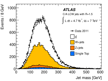
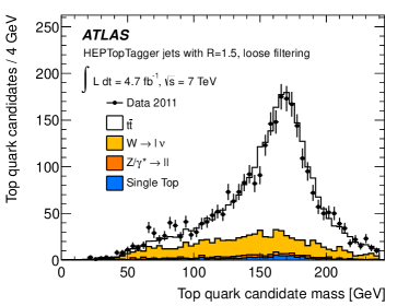
Figure 42: Detector level distributions in a selection of semileptonic $t\bar{t}$ decays of (a) the mass of $\mathrm{C/A}$ $R=1.5$ jets with $p_{\rm T}>200{\mathrm{\ Ge\kern-1.00006ptV}}$ and of the HEPTopTagger candidate mass using (b) the default-30, (c) tight, and (d) loose HEPTopTagger settings of Table 1. The $t\bar{t}$ simulation is from MC@NLO and the $W\!$+jets simulation from ALPGEN+HERWIG. From [106].

The mass of the HEPTopTagger input jets is shown in Figure 42a. These $\mathrm{C/A}$ $R=1.5$ fat jets have $p_{\rm T}>200{\mathrm{\ Ge\kern-1.00006ptV}}$ and the distribution is peaked near the top quark mass with a large width of $\approx\!160{\mathrm{\ Ge\kern-1.00006ptV}}$. The simulated distribution is shifted by $\approx\!8{\mathrm{\ Ge\kern-1.00006ptV}}$ to higher masses. This difference to the observed mass is within the typical jet mass simulation uncertainty of $5$–$6\%$ found for fat jets [106]. Approximately $50\%$ of the fat jets sample are SM $t\bar{t}$ events and the other half is dominated by $W\!$+jets events. The HEPTopTagger top quark candidate masses are shown in Figure 42b–d for different HEPTopTagger parameter settings. The default-30 settings are used in Figure 42b which shows a peak at the top quark mass that falls rapidly towards larger masses. The tail towards lower masses results from cases where not all energy associated with the top quark decay is recovered. These losses occur in the filtering and when not all decay products are contained in the fat jet. The effect on the mass distribution of tightening and loosening the filtering is shown in Figure 42c and d: tight settings enhance the tail with respect to the peak while loose settings reduce it. Which settings are optimal depends on the analysis and on the amount of background that needs to be rejected. The top candidate mass $m_{t}$ above $50{\mathrm{\ Ge\kern-1.00006ptV}}$ is well described by the simulation. The $t\bar{t}$ events are generated using MC@NLO and ALPGEN is used for $W\!$+jets events. The HEPTopTagger increases the purity from $\approx\!50\%$ $t\bar{t}$ processes before tagging to $86\%$ in the mass window $140<m_{t}<200{\mathrm{\ Ge\kern-1.00006ptV}}$.

The simulation underestimates the data at low $m_{t}$. This phase space represents the deep substructure, where three subjets with $p_{\rm T}>20{\mathrm{\ Ge\kern-1.00006ptV}}$ combine to a small invariant mass of $10$–$40{\mathrm{\ Ge\kern-1.00006ptV}}$. The subjet energy scale simulation uncertainty is expected to play an important role here and this uncertainty is not shown in the figure. The peak at low mass is removed when using the loose settings (Figure 42d). This is due to an increase of the $m_{\rm cut}$ parameter from $30$ to $70{\mathrm{\ Ge\kern-1.00006ptV}}$. As described in Section 7.7, this parameter controls the maximal mass of the substructure objects which enter the filtering procedure. Lowering this mass implies a larger number of substructure objects. A triplet of substructure objects is combined to a top quark candidate. If $m_{\rm cut}$ is too small then a fat jet that contains a hadronically decaying top quark is split into four or more substructure objects which share contributions from the three decay jets. In that case, a triplet of these objects cannot reconstruct the top quark. The value that was used in the HEPTopTagger analysis described in Section 10.2.1 is $m_{\rm cut}=50{\mathrm{\ Ge\kern-1.00006ptV}}$ which removes the peak in the top candidate mass distribution as shown below.

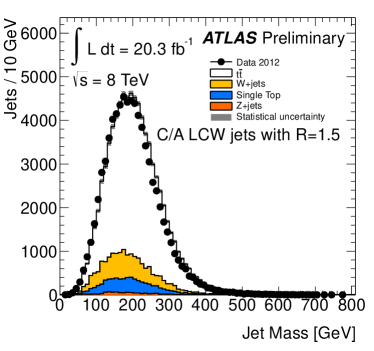
Figure 43: Detector level distributions in a selection of semileptonic $t\bar{t}$ decays with a $b$-tag of (a) the mass of $\mathrm{C/A}$ $R=1.5$ jets with $p_{\rm T}>200{\mathrm{\ Ge\kern-1.00006ptV}}$ and (b) the HEPTopTagger candidate mass using the default HEPTopTagger settings of Table 1. The $t\bar{t}$ simulation is from POWHEG+PYTHIA, the $W\!$+jets events from ALPGEN+PYTHIA, and single-top production in the $s$-channel with a leptonically decaying $W$ boson is from MC@NLO. From [102].

Figure 43a shows the fat jet mass distribution for ATLAS events from 2012 that pass the semileptonic $t\bar{t}$ event selection, including a $b$-tag to reduce the $W\!$+jets background. The top quark purity of this sample of fat jets is $86\%$. The fat jet mass exhibits a broad peak with a maximum at $180{\mathrm{\ Ge\kern-1.00006ptV}}$. The distribution predicted by the simulation is shifted towards higher masses. Between $200$ and $350{\mathrm{\ Ge\kern-1.00006ptV}}$ the shift is approximately $10{\mathrm{\ Ge\kern-1.00006ptV}}$, which corresponds to a relative change of $5\%$ at a mass of $200{\mathrm{\ Ge\kern-1.00006ptV}}$. As for 2011, this difference is covered by the typical fat jet simulation uncertainty [106]. The HEPTopTagger candidate mass, reconstructed using the default settings listed in Table 1, is shown in Figure 43b. No peak is visible at low mass due to the use of $m_{\rm cut}=50{\mathrm{\ Ge\kern-1.00006ptV}}$. The top candidate mass is well described by the simulation. The HEPTopTagger increases the top quark purity to $98\%$ in the candidate mass window $140<m_{t}<200{\mathrm{\ Ge\kern-1.00006ptV}}$. The number of top quark candidates reconstructed in this mass window in the data is $4210$. As proposed in [126], the top quark mass peak can be used to calibrate the HEPTopTagger subjets and to evaluate the subjet energy simulation uncertainty.

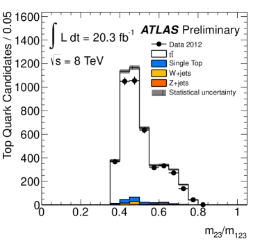
Figure 44: Detector level distributions of the HEPTopTagger substructure variables for top quark candidates that pass the HEPTopTagger procedure and have a mass between $140$ and $200{\mathrm{\ Ge\kern-1.00006ptV}}$ in a selection of semileptonic $t\bar{t}$ decays with a $b$-tag. (a) The subjet invariant mass ratio $m_{23}/m_{123}$. (b) The quantity $\arctan(m_{13}/m_{12})$. The quantities $m_{ij}$ are invariant masses of two of the three final subjets in the HEPTopTagger procedure which are ordered in $p_{\rm T}$ such that $p_{{\rm T},1}>p_{{\rm T},2}>p_{{\rm T},3}$. The $t\bar{t}$ simulation is from POWHEG+PYTHIA, the $W\!$+jets events from ALPGEN+PYTHIA, and single-top production in the $s$-channel with a leptonically decaying $W$ boson is from MC@NLO. From [102].

Distributions of substructure variables used by the HEPTopTagger to apply kinematic cuts on the three identified subjet are shown in Figure 44 for the top quark candidates with $140<m_{t}<200{\mathrm{\ Ge\kern-1.00006ptV}}$. These variables are invariant mass ratios of combinations of the three (exclusive) subjets identified in the last step of the HEPTopTagger procedure (cf. Section 7.7). For example, the variable $m_{23}$ is the invariant mass of the subleading $p_{\rm T}$ and the sub-subleading $p_{\rm T}$ subjet, and the variable $m_{123}$ is the mass of all three subjets combined. The ratio $m_{23}/m_{123}$ displayed in panel (a) shows a peak at $m_{W}/m_{t}$. This indicates that in most of the cases the leading $p_{\rm T}$ subjet corresponds to the $b$-quark (but this information is not used in the HEPTopTagger). The distribution is well described by the simulation as is the quantity $\arctan(m_{13}/m_{12})$ in panel (b).

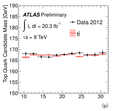
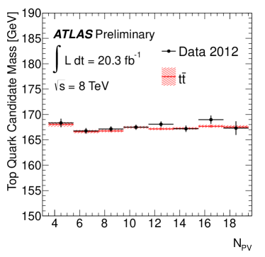
Figure 45: HEPTopTagger top candidate mass as a function of (a) the average number of interactions per bunch-crossing $\mu$ and (b) the number of reconstructed primary vertices in the event. The mass is defined as the average mass in the window $140<m_{t}<200{\mathrm{\ Ge\kern-1.00006ptV}}$ and the error bars correspond to the statistical uncertainty of the average mass. The $t\bar{t}$ simulation is from POWHEG+PYTHIA. From [102].

Figure 45 shows the reconstructed top candidate mass for different pile-up conditions. The average candidate mass in the window $140<m_{t}<200{\mathrm{\ Ge\kern-1.00006ptV}}$ is plotted as a function of the average number of interactions per bunch-crossing $\mu$ in panel (a) and as a function of the number of reconstructed primary vertices $N_{\rm PV}$ in (b). The $\mu$ and $N_{\rm PV}$ intervals are chosen such that each average mass is calculated from at least 100 entries. Within the statistical uncertainty of the average mass of approximately $\pm 1{\mathrm{\ Ge\kern-1.00006ptV}}$, the reconstructed top quark mass is not affected by pile-up energy in the full accessible range up to $\mu=31$ and $N_{\rm PV}=19$. This is also seen for the generated semileptonic $t\bar{t}$ events that have been passed through a full ATLAS detector simulation under the same pile-up conditions. The numerical value of the reconstructed top quark mass depends on the choice of the mass window and is well predicted by the simulation.

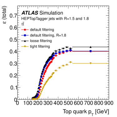
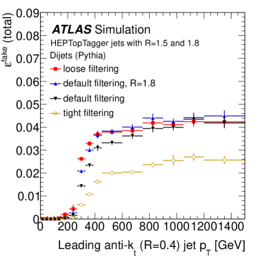
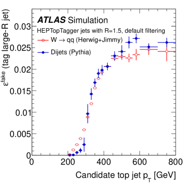
Figure 46: Simulated HEPTopTagger efficiency for different parameter settings in (a) semileptonic $t\bar{t}$ decays (MC@NLO), (b) multijet events, and (c) multijet and $W\!$+jets events. The efficiency in (a) is per top quark and shown as a function of the top quark $p_{\rm T}$. The fake rate in (b) is an event-level rate and is shown as a function of the leading anti-$k_{\rm T}$ $R=0.4$ jet $p_{\rm T}$ in the event. The fake rate in (c) is per fat jet and shown as a function of the fat jet $p_{\rm T}$. The default filtering efficiencies correspond to the default-30 settings in Table 1. From [106].

As shown above, the simulation describes the data well before and after applying the HEPTopTagger. Simulated HEPTopTagger efficiencies are presented in Figure 46. The top quark tagging efficiency per top quark is shown in panel (a) as a function of the top quark transverse momentum $p_{{\rm T},t}$. The efficiency is a product of the efficiency to find a fat jet in the event and the efficiency to tag the fat jet. The former efficiency is close to $100\%$ for $p_{{\rm T},t}>300{\mathrm{\ Ge\kern-1.00006ptV}}$. The efficiency shows a turn-on at $p_{{\rm T},t}\approx 200{\mathrm{\ Ge\kern-1.00006ptV}}$ and rises to a plateau of $\approx\!40\%$ for $p_{{\rm T},t}>500{\mathrm{\ Ge\kern-1.00006ptV}}$. The turn-on is a geometric effect, with more top quark decay products contained in the fat jet at larger $p_{\rm T}$. This is evident from a comparison with the efficiency obtained when using $\mathrm{C/A}$ $R=1.8$ fat jet which is larger in the turn-on but equal to the $R=1.5$ efficiency in the plateau. The plateau is given by the internal HEPTopTagger inefficiencies associated with the procedure that identifies the hard substructure (mass drop), the filtering, and the kinematic selection. Different choices of the HEPTopTagger parameters allow to tighten or loosen the top quark selection to achieve an optimal signal-to-background ratio (S/B). Typically tight settings are needed when the background is large and the fake rate needs to be kept as small as possible. Loose settings are possible if the background is small or has been reduced to a low level through other selection cuts. In this case a high efficiency is preferred. The tight and loose parameters are listed in Table 1. The tight settings include more aggressive filtering, through the use of a smaller filtering radius and a smaller number of kept filtered jets, and a smaller $W$ boson mass window. For the loose settings, the filtering is relaxed (more jets are accepted) and the $W$ boson mass window is widened. The tight HEPTopTagger settings reduce the efficiency to $30\%$ while the loose settings increase it to $44\%$.

The HEPTopTagger fake rate is shown in Figure 46b for multijet events. This is a per-event rate with no event selection cuts other than the HEPTopTagger applied. The rate is shown as a function of the leading anti-$k_{\rm T}$ $R=0.4$ jet $p_{\rm T}$ in the event to facilitate comparisons between taggers that use different definitions of fat jets. The fake rate shows a turn-on at $\approx\!200{\mathrm{\ Ge\kern-1.00006ptV}}$ and rises to $\approx\!4\%$ at $800{\mathrm{\ Ge\kern-1.00006ptV}}$ and continues to rise slowly with $p_{\rm T}$. This turn-on is an effect of increased hard QCD radiation at large parton $p_{\rm T}$ which increases the chance to fake the three prong structure of hadronic top quark decay. With tight settings, the fake rate is reduced from $4\%$ to $2.5\%$ at high $p_{\rm T}$. The fake rate with loose settings differs from that obtained with the default settings only in the turn-on.

Figure 46c shows the fat jet tagging efficiency as a function of the fat jet $p_{\rm T}$ for multijet events and $W\!$+jets events in which the $W$ boson decays hadronically. For both types of events, the fake rate is $\approx\!2.5\%$ for fat jet $p_{\rm T}>500{\mathrm{\ Ge\kern-1.00006ptV}}$, while the turn-on begins $\approx\!50{\mathrm{\ Ge\kern-1.00006ptV}}$ earlier for $W\!$+jets events. This is expected because $W\rightarrow qq$ decay provides a hard 2-prong structure that is not present in most QCD jets.

9.2 Performance comparison of top tagging approaches

Parts of this section are taken from section 6 of [102], having been written by the author. This section compares the performance of the HEPTopTagger with that of cuts on substructure variables as presented in [102]. The comparison is made in the context of searches for resonances in the $t\bar{t}$ invariant mass spectrum using the benchmark model of a $Z^{\prime}$ boson with a mass of $1.75{\mathrm{\ Te\kern-1.00006ptV}}$. This mass is just above the current published exclusion limit [127] discussed in Section 10.1.

The boosted top quark tagging efficiency and the rejection of jets arising from light quarks or gluons are determined from simulation. High $p_{\rm T}$ top quarks are obtained from PYTHIA 8 $Z^{\prime}$ events with $m_{\rm Z^{\prime}}=1.75{\mathrm{\ Te\kern-1.00006ptV}}$, in which the $Z^{\prime}$ boson decays exclusively to $t\bar{t}$. To estimate the background rejection, a simulated inclusive jet sample from PYTHIA 8 is used.

The direct comparison at the fat jet level is difficult because of different fat jet definitions: the HEPTopTagger uses $\mathrm{C/A}$ fat jets while the variables are calculated for trimmed anti-$k_{\rm T}$ jets. The cleanest comparison would be at the event level but the approach taken in [102] is to geometrically match the fat jets. Samples of truth level particle jets are defined for signal and background by requiring at least one $\mathrm{C/A}$ $R=1.2$ jet and at least one trimmed anti-$k_{\rm T}$ $R=1.0$ jet, both with $p_{\rm T}>150{\mathrm{\ Ge\kern-1.00006ptV}}$ and $|\eta|<1.2$. The trimming parameters are $f_{\rm cut}=5\%$ and $R_{\rm sub}=0.3$. For the signal, the truth level requirements include a hadronically decaying top quark with $p_{\rm T}>150{\mathrm{\ Ge\kern-1.00006ptV}}$ and $|\eta|<1.2$ within $\Delta R_{\eta}<0.75\times R$ of the leading $p_{\rm T}$ fat jet of either type. At the reconstruction level, events are required to contain at least one $\mathrm{C/A}$ $R=1.2$ jet and at least one trimmed anti-$k_{\rm T}$ $R=1.0$ jet, both with $p_{\rm T}>550{\mathrm{\ Ge\kern-1.00006ptV}}$ and $|\eta|<1.2$. Both reconstructed fat jets are required to be matched within $\Delta R_{\eta}<0.75\times R$ to the corresponding truth level particle jet of the same algorithm and $R$ parameter. The reconstructed $\mathrm{C/A}$ and anti-$k_{\rm T}$ fat jets are also required to be within $\Delta R_{\eta}<0.75$ of one another to ensure that the performance of the different taggers is measured using input objects from the same top quark decay.

The shape of the detector level fat jet $p_{\rm T}$ distribution is shown in Figure 47 for signal and background. For the signal, the spectrum reflects the Jacobian peak structure of the top quark $p_{\rm T}$ distribution and peaks near $m_{\rm Z^{\prime}}/2$. The $p_{\rm T}$ of the $\mathrm{C/A}$ jets is greater on average than the $p_{\rm T}$ of geometrically matched trimmed anti-$k_{\rm T}$ jets.

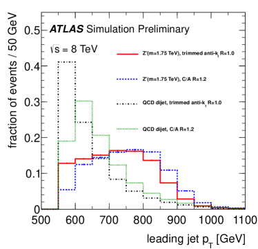
Figure 47: The fat jet $p_{\rm T}$ spectra for signal ($Z^{\prime}\rightarrow t\bar{t}$) and background (multijets) that are used for the tagging comparison. The events are generated with PYTHIA 8. From [102].

Six different substructure variable based taggers are compared, all based on trimmed anti-$k_{\rm T}$ $R=1.0$ jets:

• substructure tagger I: $\sqrt{d_{12}}>40{\mathrm{\ Ge\kern-1.00006ptV}}$ (labelled ‘$\sqrt{d_{12}}$ tagger I’ in Figure 48)

• substructure tagger II: trimmed anti-$k_{\rm T}$ $R=1.0$ mass $m^{\rm jet}>100{\mathrm{\ Ge\kern-1.00006ptV}}$ (labelled ‘$m^{\rm jet}$ tagger II’)

• substructure tagger III: $m^{\rm jet}>100{\mathrm{\ Ge\kern-1.00006ptV}}$, $\sqrt{d_{12}}>40{\mathrm{\ Ge\kern-1.00006ptV}}$ (labelled ‘$m^{\rm jet}$ & $\sqrt{d_{12}}$ tagger III’)

• substructure tagger IV: $m^{\rm jet}>100{\mathrm{\ Ge\kern-1.00006ptV}}$, $\sqrt{d_{12}}>40{\mathrm{\ Ge\kern-1.00006ptV}}$, $\sqrt{d_{23}}>10{\mathrm{\ Ge\kern-1.00006ptV}}$
  (labelled ‘$m^{\rm jet}$ & $\sqrt{d_{12}}$ & $\sqrt{d_{23}}$ tagger IV’)

• substructure tagger V: $m^{\rm jet}>100{\mathrm{\ Ge\kern-1.00006ptV}}$, $\sqrt{d_{12}}>40{\mathrm{\ Ge\kern-1.00006ptV}}$, $\sqrt{d_{23}}>20{\mathrm{\ Ge\kern-1.00006ptV}}$
  (labelled ‘$m^{\rm jet}$ & $\sqrt{d_{12}}$ & $\sqrt{d_{23}}$ tight tagger V’)

• substructure tagger VI: $\sqrt{d_{12}}>40{\mathrm{\ Ge\kern-1.00006ptV}}$, $0.4<\tau_{21}<0.9$, $\tau_{32}<0.65$
  (labelled ‘$\sqrt{d_{12}}$ & N-subjettiness tagger VI’)

Tagger III has been used in searches for $t\bar{t}$ resonances in the semileptonic channel [127, 128]. The others are compared to study the performance of different combinations of substructure variables. The HEPTopTagger performance is evaluated using the default, tight, and loose parameters specified in Table 1. The $\mathrm{C/A}$ fat jet radius parameter $R$ was lowered from the nominal $1.5$, for which the HEPTopTagger was designed and optimised, to $1.2$. One reason is that the large $p_{\rm T}$ of the top quarks under study leads to a collimation of the decay products to a smaller cone. The second motivation is to make the radius parameter more similar to the one used for the trimmed fat jets.

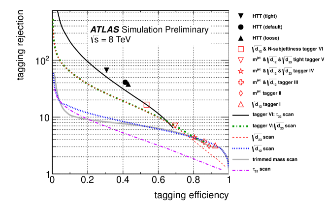
Figure 48: Comparison of the simulated fat top jet tagging efficiency and fat light quark/gluon jet rejection (defined as the inverse of the fake rate) of different taggers. The top jets originate from the decay of a $Z^{\prime}$ boson of mass $1.75{\mathrm{\ Te\kern-1.00006ptV}}$ and the background is given by multijet events. All events are generated with PYTHIA 8. The fat jet $p_{\rm T}$ is required to be greater than $550{\mathrm{\ Ge\kern-1.00006ptV}}$. All substructure taggers and scans use trimmed anti-$k_{\rm T}$ $R=1.0$ jets. The HEPTopTagger (points labelled ‘HTT’) uses $\mathrm{C/A}$ $R=1.2$ jets that are geometrically matched to the anti-$k_{\rm T}$ jets. From [102].

Figure 48 shows a comparison of the efficiency $\varepsilon$ for tagging fat jets that contain a top quark and the rejection of fat jets originating from hard light quarks or gluons. The rejection is defined as the inverse of the fake rate. The best rejection of all studied taggers is obtained with the HEPTopTagger when using the tight settings, which, however, also results in the smallest efficiency. Loosening the HEPTopTagger parameters improves the efficiency at a cost in rejection. The performances obtained from the default and loose parameters differ only slightly.

The substructure tagger III has a high efficiency and a small rejection. Such a working point is typically used in analyses in which the background has already been reduced by measures not related to jet substructure, such as the requirement of a final state lepton.

Tagger I is tagger III without the requirement on the trimmed fat jet mass and yields a higher efficiency but worse rejection. The cut on $\sqrt{d_{12}}$ has been varied from the nominal $40{\mathrm{\ Ge\kern-1.00006ptV}}$ for tagger I, resulting in the continuous curve labelled ‘$\sqrt{d_{12}}$ scan’, which crosses the points for taggers III and IV. This indicates that, for the signal and background fat jets under study here, the mass cut can be dropped from tagger III without compromising its performance. Adding a cut $\sqrt{d_{23}}>10{\mathrm{\ Ge\kern-1.00006ptV}}$ (as in tagger IV) also does not help in separating signal from background. A larger cut value of $20{\mathrm{\ Ge\kern-1.00006ptV}}$ in combination with the mass cut, however, increases the rejection as can be seen from the position of the tagger V point in relation to the curve. The variation of the $m^{\rm jet}$ cut in tagger II (‘trimmed mass scan’) gives a performance very similar to the one from the $\sqrt{d_{12}}$ cut, indicating that the two variables are strongly correlated.

Also investigated was the impact of a standalone cut on $\sqrt{d_{23}}$. The performance that results from varying the minimal required $\sqrt{d_{23}}$ (‘$\sqrt{d_{23}}$ scan’) offers better rejection than a cut on $\sqrt{d_{12}}$ for $\varepsilon\lesssim 75\%$, almost reaching that of tagger V which uses a combination of cuts on $\sqrt{d_{23}}$, $\sqrt{d_{12}}$, and the mass, suggesting that the latter two cuts can be dropped at minimal expense. The $\sqrt{d_{23}}$ cut in tagger V has been varied while keeping the other cuts fixed (‘tagger V: $\sqrt{d_{23}}$ scan’), resulting in a performance which differs from that of $\sqrt{d_{23}}$ only for $\varepsilon\gtrsim 70\%$ where it gives better rejection. Variations of the other cuts in tagger V (one at a time, fixing the other cut-offs to their nominal values) do not improve the performance compared to the $\sqrt{d_{23}}$ variation.

A standalone cut on the $N$-subjettiness variable $\tau_{32}$ (‘$\tau_{32}$ scan’) yields a significantly worse performance than cuts on splitting scales. Combining $N$-subjettiness and splitting scale information (tagger VI), however, gives the best performance of all substructure variable based taggers for $\varepsilon\lesssim 60\%$. By varying the $\tau_{32}$ cut in tagger VI (‘tagger VI: $\tau_{32}$ scan’), rejections close to those of the HEPTopTagger can be achieved: for $\varepsilon\approx 40\%$ ($30\%$) the rejection is $\approx 0.75$ ($0.7$) times that of the HEPTopTagger.

For the present study, the performance of taggers based on substructure variables is driven by cuts on splitting scales. For $\varepsilon\gtrsim 75\%$, a standalone cut on the first splitting scale $\sqrt{d_{12}}$ gives the best performance. At lower efficiencies, the second splitting scale $\sqrt{d_{23}}$ is the variable that in a standalone cut best separates signal from background. Adding $N$-subjettiness information increases the performance, whereas an additional cut on the trimmed fat jet mass does not help significantly.

The studied substructure variable taggers achieve higher efficiencies than the HEPTopTagger. Compared at the same efficiency, however, they yield a smaller rejection, making the HEPTopTagger the algorithm of choice for analyses in which the multijet background is large. Finding the best performance of the substructure taggers that are based on several variables requires a multi-dimensional variation of the cut values. The top quark taggers presented here provide a broad spectrum of working points, and the best choice for any particular analysis depends on the needed efficiency and rejection.

9.3 Top tagging in high jet multiplicity environments

In this section the performance of top tagging approaches is studied in LHC events with a large number of jets. Such an environment is typically encountered in scenarios of New Physics models where new massive particles decay with large hadronic branching fractions. For the present study, $\sqrt{s}=14{\mathrm{\ Te\kern-1.00006ptV}}$ $pp$ collisions are used and small-$R$ jets are constructed using the anti-$k_{\rm T}$ algorithm with $R=0.4$. Fat jets are constructed using the $\mathrm{C/A}$ algorithm with $R=1.5$, and the efficiency and rejection of the HEPTopTagger is compared with those of cuts on the fat jet mass, $p_{\rm T}$, and the multiplicity of hard substructure objects inside the fat jet. In a real analysis, these substructure techniques would be combined with other requirements to increase the signal sensitivity. Many such requirements, e.g., cuts on $/{\!\!\!\!E_{\rm T}}$ and $b$-tagging, factorise because the HEPTopTagger does not use the corresponding variables and the fat jet variables are not or only weakly correlated with those variables. The approach taken in this study is therefore to not consider other cuts and to look at the significance improvement rather than absolute values of $S/\sqrt{B}$.

A supersymmetric extension of the SM ($R$-parity conserving SUSY) is used as the benchmark model for the comparison. Gluinos are pair-produced and decay to four top quarks and two neutralinos, as shown in Figure 49a. Each gluino decays according to $\tilde{g}\rightarrow\bar{t}\,\tilde{t}\rightarrow\bar{t}t\tilde{\chi}^{0}_{1}$, in which $\tilde{\chi}^{0}_{1}$ is the lightest supersymmetric particle (LSP). The masses chosen for the study are $m_{\tilde{g}}=1.3{\mathrm{\ Te\kern-1.00006ptV}}$, $m_{\tilde{t}}=2.5{\mathrm{\ Te\kern-1.00006ptV}}$, and $m_{\tilde{\chi}^{0}_{1}}=100{\mathrm{\ Ge\kern-1.00006ptV}}$ with the top squark $\tilde{t}$ from gluino decay being off-shell. These signal events are generated using MadGraph+HERWIG++.

Figure 49: (a) Feynman diagram for the process $pp\rightarrow\tilde{g}\tilde{g}\rightarrow 4t\,2\tilde{\chi}^{0}_{1}$. (b) Top quark $p_{\rm T}$ for $10\leavevmode\nobreak\ {\rm fb}^{-1}$ of $\sqrt{s}=14{\mathrm{\ Te\kern-1.00006ptV}}$ $pp$ collisions with $m_{\tilde{g}}=1.3{\mathrm{\ Te\kern-1.00006ptV}}$, $m_{\tilde{t}}=2.5{\mathrm{\ Te\kern-1.00006ptV}}$, $m_{\tilde{\chi}^{0}_{1}}=100{\mathrm{\ Ge\kern-1.00006ptV}}$. The events are generated with MadGraph+HERWIG++.

The $p_{\rm T}$ spectrum of the top quarks is shown in Figure 49b were the event counts correspond to $10\leavevmode\nobreak\ {\rm fb}^{-1}$. The quarks are moderately boosted, with the average leading $p_{\rm T}$ being $504{\mathrm{\ Ge\kern-1.00006ptV}}$ and the average subleading $p_{\rm T}$ being $326{\mathrm{\ Ge\kern-1.00006ptV}}$. The events are processed with the Delphes simulation of the ATLAS detector. The $p_{\rm T}$ distribution of anti-$k_{\rm T}$ $R=0.4$ jets reconstructed in the events is shown in Figure 50a.

(a) signal

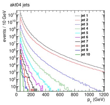
(b) background

Figure 50: The $p_{\rm T}$ distributions of the ten leading $p_{\rm T}$ anti-$k_{\rm T}$ $R=0.4$ jets in events of (a) the SUSY benchmark model (from MadGraph+HERWIG++) and (b) the multijet background (from PYTHIA 8). The events correspond to $10\leavevmode\nobreak\ {\rm fb}^{-1}$ of $\sqrt{s}=14{\mathrm{\ Te\kern-1.00006ptV}}$ $pp$ collisions and have been passed through the Delphes simulation of the ATLAS detector.

The background for the study are multijet events generated with PYTHIA 8.175 and the $p_{\rm T}$ spectra are shown in Figure 50b. A leading-order $2\!\!\rightarrow\!\!2$ parton generator, supplemented with a parton shower to approximate higher orders particle emission, may not be the optimal tool to simulate the multijet background. Multileg generators like SHERPA (up to 6 partons in the matrix element) and MadGraph (up to 4 partons) might be better choices although both also rely on the parton shower for higher multiplicity. The best approach is to take the multijet distributions from data as done in the high jet multiplicity ATLAS analysis discussed in Section 10.4. The simulations used in this study do not include pile-up. No grooming techniques are therefore used to clean the fat jets.

(a) signal

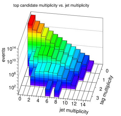
(b) background

Figure 51: The HEPTopTagger top quark candidate multiplicity as a function of the anti-$k_{\rm T}$ $R=0.4$ jet multiplicity in $10\leavevmode\nobreak\ {\rm fb}^{-1}$ of $\sqrt{s}=14{\mathrm{\ Te\kern-1.00006ptV}}$ $pp$ collision events that have been passed through the Delphes simulation of the ATLAS detector for (a) the SUSY benchmark model (from MadGraph+HERWIG++) and (b) multijet background events (from PYTHIA 8).

The HEPTopTagger top quark candidate multiplicity is shown in Figure 51 as a function of the multiplicity $N_{\rm jet}$ of anti-$k_{\rm T}$ $R=0.4$ jets with $p_{\rm T}>50{\mathrm{\ Ge\kern-1.00006ptV}}$ for signal and background events when using the default HEPTopTagger settings. The average $N_{\rm jet}$ in signal events is $7.6$ while the background $N_{\rm jet}$ spectrum is steeply falling. For signal and background, the $N_{\rm jet}$ distribution is shifted towards higher values the more top tags are found. In other words, the probability for a top tag rises with the number of jets in the event. This behaviour can be understood as follows. The HEPTopTagger looks for hard substructure objects inside the fat jet. It then tries all permutations of three of the substructure objects and looks if this triplet combines to a top quark. E.g., the (filtered) triplet has to fulfil the top quark mass constraint and two subjets have to fulfil the $W$ boson mass constraint. The larger the small-$R$ jet multiplicity, the higher the number of hard substructure objects and the probability increases that a triplet is found which satisfies the kinematic cuts (hits the mass windows).

The observed feature, that the tagging probability rises with the jet multiplicity is not limited to the HEPTopTagger. It is a general feature that affects all top taggers. The reason is that the more jets are in the event, the larger the probability that a combination of jets looks like hadronic top quark decay. The chance that the structure of a fat jet resembles hadronic top quark decay is higher if the fat jet has more subjets.

Experimentally, a minimal $N_{\rm jet}$ cut is more natural than a requirement of exactly $N_{\rm jet}$ small-$R$ jets. Measuring an exact number of jets is harder and the systematic uncertainties are larger. Therefore, in the rest of this section, distributions like those in Figure 51 are integrated over $N_{\rm jet}$, starting from a minimal value.

Figure 52a shows the HEPTopTagger efficiency for at least one and at least two top tags in signal and background events as a function of the minimal number of required jets. The efficiency to find at least one top tag in SUSY events rises from $44\%$ at $N_{\rm jet}\geq 4$ to $60\%$ for $N_{\rm jet}\geq 12$. The efficiency to have at least a double-tag rises from $6\%$ to $18\%$. The rise is due to mass window hits which are more likely at higher jet multiplicity. This effect is more dramatic for the fake rate which rises from $10^{-4}$ at $N_{\rm jet}\geq 2$ to $16\%$ at $N_{\rm jet}\geq 8$ for single-tags.

The rise of the signal efficiency is much smaller than that of the fake rate. The explanation is that for signal, the fat jets contain top quark decays and the efficiency is already high at low $N_{\rm jet}$. The plateau efficiency of the HEPTopTagger is $\approx\!40\%$ when using full detector simulation (Section 9.1). The HEPTopTagger inefficiency of $\approx\!60\%$ is due to mass drop filtering and mass cuts. High jet multiplicity in signal events helps reduce this inefficiency. E.g., a signal event that would have escaped detection because the top quark candidate has a mass larger than the maximum allowed value can be tagged if the excess energy is removed in the form of a radiated hard gluon. This gluon then gives rise to another jet in the event. The efficiency increase from such processes is relatively small because the mass windows are already designed for high signal efficiency.

For background events, however, QCD radiation makes the difference between almost no fat jet structure, where most of the energy is carried by one subjet, and structure that resembles top quark decay. The fake rate therefore depends strongly on the number of small-$R$ jets in the event.

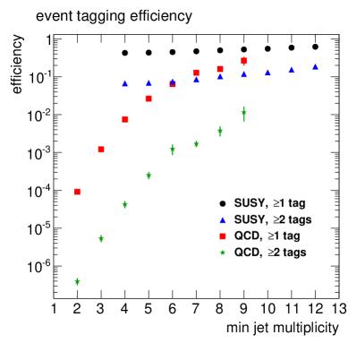
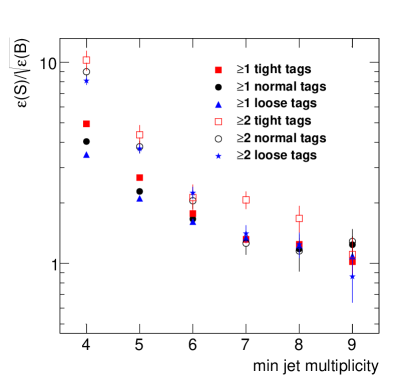
Figure 52: (a) The HEPTopTagger efficiency to tag signal events (SUSY, from MadGraph+HERWIG++) and background events (QCD jets, from PYTHIA 8) with at least one or at least two tags as a function of the minimal required number of anti-$k_{\rm T}$ $R=0.4$ jets with $p_{\rm T}>50{\mathrm{\ Ge\kern-1.00006ptV}}$. The default HEPTopTagger settings from Table 1 are used. (b) The ratio of the signal efficiency to the square root of the background efficiency for different HEPTopTagger settings. The events have been passed through the Delphes simulation of the ATLAS detector.

The ratio of the signal efficiency to the square root of the background efficiency is shown in Figure 52b. This ratio corresponds to the improvement in the significance $S/\sqrt{B}$ from applying the HEPTopTagger. The HEPTopTagger is most useful at low jet multiplicity. For $N_{\rm jet}\geq 4$, the improvement is by a factor of $\approx\!10$ for double-tags. Single-tags with tight HEPTopTagger settings give a factor of $5$ and default and loose settings give $4$ and $3.5$, respectively. The best performance is obtained with tight settings which suppress the background most. However, the background jet multiplicity spectrum is steeply falling and requiring more jets helps more than HEPTopTagger tags as long as the signal is preserved. Most of the signal events contain at least seven $R=0.4$ jets and for $N_{\rm jet}\geq 7$ the improvement from a tight double-tag is a factor of $\approx\!2$.

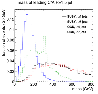
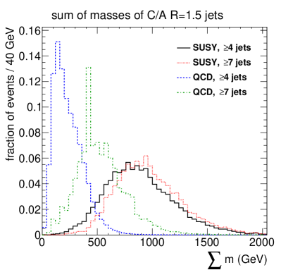
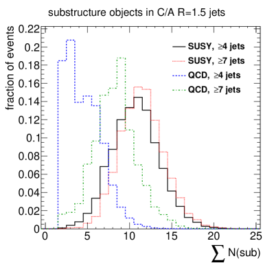
Figure 53: Normalised distributions in signal (SUSY, from MadGraph+HERWIG++) and background (QCD, from PYTHIA 8) events of $\mathrm{C/A}$ $R=1.5$ fat jet quantities for two anti-$k_{\rm T}$ $R=0.4$ jet multiplicities: (a) leading fat jet $p_{\rm T}$, (b) mass of the leading $p_{\rm T}$ fat jet, (c) sum of masses of all fat jets, (d) sum of the number of substructure objects in all fat jets. The substructure objects are obtained by the HEPTopTagger after the mass drop requirement with $\mu=80\%$ and $m_{\rm cut}=50{\mathrm{\ Ge\kern-1.00006ptV}}$). The spikes in the background distribution for $N_{\rm jet}\geq 7$ are statistical fluctuations. The events have been passed through the Delphes simulation of the ATLAS detector.

For comparison with the performance of the HEPTopTagger, cuts on fat jet quantities, detailed below, are used to separate signal and background events. Figure 53 shows the distributions of the $\mathrm{C/A}$ $R=1.5$ fat jet quantities. The distributions are shown for $N_{\rm jet}\geq 4$ and $N_{\rm jet}\geq 7$. Most of the signal events have $N_{\rm jet}\geq 7$ (Figure 51a). This implies that the signal fat jets for $N_{\rm jet}\geq 4$ and those for $N_{\rm jet}\geq 7$ have almost the same number of subjets. The subjets determine the kinematics of the fat jet. This is the reason why the distributions of the kinematic variables and the number of substructure objects do not change much for the signal fat jets when $N_{\rm jet}$ is increased. The situation is quite different for fat jets in background events. These events have a falling jet multiplicity spectrum (Figure 51b) and the fat jets in events with $N_{\rm jet}\geq 4$ have fewer subjets than those in events with $N_{\rm jet}\geq 7$. Consequently, the kinematics of background fat jets becomes more signal-like at high $N_{\rm jet}$.

Figure 53a shows the leading fat jet $p_{\rm T}$. As expected, the background distribution is less well separated from the signal at high jet multiplicities. A cut $p_{\rm T}>500{\mathrm{\ Ge\kern-1.00006ptV}}$ is used to enhance signal events. This cut and the cuts on the other fat jet quantities are chosen to ensure a high signal efficiency of at least $50\%$. The leading $p_{\rm T}$ fat jet mass is shown in panel (b) and the sum of the masses of all fat jets in the event in panel (c). Cuts $m>350{\mathrm{\ Ge\kern-1.00006ptV}}$ and $\sum m>800{\mathrm{\ Ge\kern-1.00006ptV}}$ are used, respectively. The fat jet mass sum has been proposed in [129] to select top quark events in high multiplicity environments. The sum $\sum N_{\rm sub}$ of the number of substructure objects obtained by the HEPTopTagger after the mass drop requirement ($\mu=80\%,m_{\rm cut}=50{\mathrm{\ Ge\kern-1.00006ptV}}$) in all fat jets in the event is shown in (d). A cut $\sum N_{\rm sub}>10$ is used. This variable is inspired by [130] in which the counting of subjets has been proposed as an effective discriminant. Systematic uncertainties on the fat jet mass and $p_{\rm T}$, and on the HEPTopTagger subjet calibrations have only a small impact on the efficiency: the relative uncertainty on the efficiency is a few percent for all investigated methods.

The significance improvement with these cuts is shown in Figure 54. The leading $p_{\rm T}$ fat jet mass cut and the cut on the number of substructure objects yield similar improvements which are the smallest of all tested approaches. The best improvement is obtained with the cut on the sum of the fat jet masses. At small $N_{\rm jet}$, this method is superior to all other methods, reaching an improvement by a factor of more than ten for $N_{\rm jet}\geq 4$. For $N_{\rm jet}\geq 7$ and at higher multiplicities, the cuts on the leading fat jet $p_{\rm T}$ and the tight HEPTopTagger double-tag yield similar results. The significance is improved by the fat jet mass sum method by factors 2.2, 1.6, 1.4 for $N_{\rm jet}\geq 7$, $8$, $9$, respectively. This method is used in the high multiplicity ATLAS analysis discussed in Section 10.4.

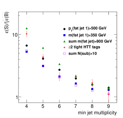
Figure 54: The ratio of the efficiency for signal and the square root of the background efficiency as a function of the minimal anti-$k_{\rm T}$ $R=0.4$ jet multiplicity in the event for different top tagging methods. The SUSY signal events are generated with MadGraph+HERWIG++ and the background multijet events with PYTHIA 8. The events have been passed through the Delphes simulation of the ATLAS detector.

10 Searches for New Physics using Boosted Top Quarks

This section discusses analyses that have been carried out using jet structure techniques to identify boosted top quarks. The first analyses of this type at the LHC looked for $t\bar{t}$ resonances, both in the semileptonic decay channel, in which one of the top quarks decays into a $W$ boson that decays into a lepton and a neutrino and the other $W$ boson decays hadronically, and in the (fully) hadronic channel.

The analyses use different methods to identify boosted top quarks and are compared using the upper limits they give for the production of new particles in two benchmark models of New Physics: topcolor (cf. Section 2.4) and warped extra dimensions (Section 2.5). Both models predict new particles (the $Z^{\prime}$ boson and the Kaluza-Klein gluon, respectively) that decay to $t\bar{t}$. The first analysis discussed in Section 10.1 compares a boosted top quark selection with a conventional top quark selection and details the advantages of either method.

Analyses that searched for a topcolor $Z^{\prime}$ boson were also carried out at the Tevatron [131, 132, 133, 134]. They used conventional top quark reconstruction because Tevatron top quarks are not boosted enough to benefit from substructure techniques. A narrow leptophobic topcolor $Z^{\prime}$ boson is excluded by the Tevatron data for masses smaller than $\approx\!900{\mathrm{\ Ge\kern-1.00006ptV}}$ at 95% confidence level.

The section also discusses a search for supersymmetry which employs boosted top quark identification.

10.1 $t\bar{t}$ resonances in the semileptonic decay channel

The best published limits on $t\bar{t}$ resonances decaying in the semileptonic channel are reported in [127] using $4.7$ fb^-1 of ATLAS data taken at $\sqrt{s}=7\,{\mathrm{\ Te\kern-1.00006ptV}}$. The analysis aims at reconstructing the decay chain $t\bar{t}\rightarrow bl\nu\,bqq$ with one top quark decaying leptonically and the other hadronically. A fat jet selection (called boosted selection) is compared with a conventional top quark selection that is based on small-$R$ jets (resolved selection).

The boosted selection requires events to have at least one anti-$k_{\rm T}$ $R=1.0$ fat jet with $p_{\rm T}>350{\mathrm{\ Ge\kern-1.00006ptV}}$, $|\eta|<2$, and $m>100{\mathrm{\ Ge\kern-1.00006ptV}}$. The constituents of the leading $p_{\rm T}$ fat jet are reclustered using the $k_{\rm T}$ jet algorithm and the $k_{\rm T}$ splitting scale $\sqrt{d_{12}}$ is required to be larger than $40{\mathrm{\ Ge\kern-1.00006ptV}}$. The events are triggered with an anti-$k_{\rm T}$ $R=1.0$ jet trigger with a threshold $p_{\rm T}$ of $300{\mathrm{\ Ge\kern-1.00006ptV}}$ which is $99\%$ efficient for the fat jets used in the analysis.

The resolved selection uses anti-$k_{\rm T}$ $R=0.4$ jets. Events are required to contain at least three jets with $p_{\rm T}>25{\mathrm{\ Ge\kern-1.00006ptV}}$ and $|\eta|<2.5$. One of these jets must have a mass larger than $60{\mathrm{\ Ge\kern-1.00006ptV}}$, the rationale being that it contains the two $W$ boson decay jets. If no jet passes this mass requirement, then an additional small-$R$ jet is required. The events are triggered by a single lepton trigger.

For both selections, every event has to have at least one anti-$k_{\rm T}$ $R=0.4$ jet with $p_{\rm T}>25{\mathrm{\ Ge\kern-1.00006ptV}}$ and $|\eta|<2.5$ that is tagged as a $b$-jet. Decays of $W$ bosons to electrons or muons are selected by applying common lepton and missing transverse energy ($/{\!\!\!\!E_{\rm T}}$) requirements.

For the boosted selection, the four-momentum of the leading $p_{\rm T}$ fat jet is taken to correspond to the four-momentum of the hadronically decaying top quark candidate. The four-momentum of the semileptonically decaying top quark candidate is reconstructed using the lepton, the small-$R$ jet closest to the lepton, the $/{\!\!\!\!E_{\rm T}}$ vector, and a $W$ boson mass constraint to calculate the longitudinal component of the missing momentum. The invariant mass $m_{t\bar{t}}$ is then calculated from the four-momenta of the two reconstructed top quarks.

For the resolved selection, all possible associations of anti-$k_{\rm T}$ $R=0.4$ jets with $p_{\rm T}>20{\mathrm{\ Ge\kern-1.00006ptV}}$ to two top quark candidates are tried and the one that gives the smallest $\chi^{2}$ when applying top quark and $W$ boson mass constraints is chosen to calculate $m_{t\bar{t}}$.

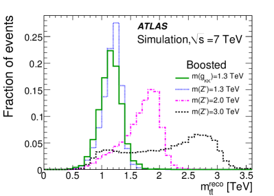
Figure 55: The reconstructed invariant mass $m_{t\bar{t}}$ using simulated ATLAS events with decays $Z^{\prime}(g_{\rm KK})\rightarrow t\bar{t}\rightarrow bl\nu\,bqq$ for reconstructions based on (a) small-$R$ jets and (b) fat jets. The $Z^{\prime}$ events are generated with PYTHIA and the $g_{\rm KK}$ events with MadGraph+PYTHIA. From [127].

Figure 55 shows the reconstructed $m_{t\bar{t}}$ spectrum for simulated events with decays of $Z^{\prime}$ bosons and Kaluza-Klein gluons of different masses. The mass resolution of the fat jet method is much better for masses larger than $0.8{\mathrm{\ Te\kern-1.00006ptV}}$. The efficiency of the boosted selection for finding $t\bar{t}$ pairs is comparable to that of the resolved selection for $m_{t\bar{t}}^{\rm true}\approx 1{\mathrm{\ Te\kern-1.00006ptV}}$ and performs better for larger masses.

In [127], the following strategy is adopted to maximise the sensitivity: if an event passes the boosted selection then $m_{t\bar{t}}$ is calculated using the fat jet; if the event fails the boosted selection but passes the resolved selection then $m_{t\bar{t}}$ is reconstructed from the small-$R$ jets. The analysis is also split into an electron and a muon channel. The selection for muons is twice as efficient because the probability to fake a muon signal is lower and therefore a less stringent cut could be applied on $/{\!\!\!\!E_{\rm T}}$, and because electron calorimeter clusters have to be separated from hadronic clusters based on cuts which leads to an inherent smaller reconstruction efficiency. The efficiency to select events with $Z^{\prime}$ boson decays with muons is larger than $8\%$ for $m_{Z^{\prime}}>1.5{\mathrm{\ Te\kern-1.00006ptV}}$ when using fat jets.

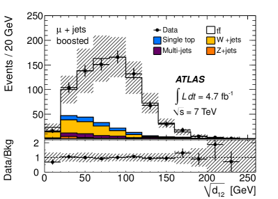
Figure 56: The $k_{\rm T}$ splitting scale $\sqrt{d_{12}}$, calculated by ATLAS for the constituents of anti-$k_{\rm T}$ $R=1.0$ jets in $t\bar{t}$ events with a muon. The simulated $t\bar{t}$ events are from MC@NLO. The $W\!$+jets events are generated with ALPGEN+HERWIG. The multijet contribution is determined from data. From [127].

Figure 56 shows the $k_{\rm T}$ splitting scale $\sqrt{d_{12}}$ for the leading $p_{\rm T}$ fat jet in muon events which pass the boosted selection (the cut on $\sqrt{d_{12}}$ has been omitted to display the full spectrum). The background from $W\!$+jets events and multijet events has a smaller fat jet splitting scale than $t\bar{t}$ events and is reduced by the cut $\sqrt{d_{12}}>40{\mathrm{\ Ge\kern-1.00006ptV}}$. The SM $t\bar{t}$ background is taken from simulation (MC@NLO) as is the $m_{t\bar{t}}$ shape of the $W\!$+jets background (ALPGEN+HERWIG). The normalisation of the $W\!$+jets background is obtained by scaling to the observed charge asymmetry in data. Processes other than $W\!$+jets give equal numbers of positively and negatively charged leptons. The MC is scaled by a factor $(N_{W^{+}}-N_{W^{-}})_{\rm Data}/(N_{W^{+}}-N_{W^{-}})_{\rm MC}$. The uncertainty of this factor is $10$–$20\%$, depending on the selection, and is compatible with unity. The multijet background is obtained from data by deriving lepton efficiencies and mis-tag rates in control samples that are signal-enriched (dileptons in $Z$ boson mass window) or dominated by multijets, respectively. The largest contribution to the relative systematic uncertainty of $25\%$ on the yield of SM events is $17\%$ from the uncertainties on the energy and mass scales of the fat jets.

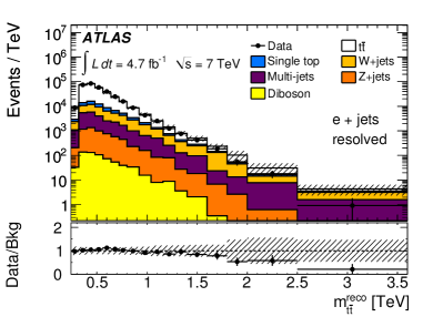
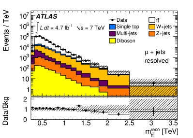
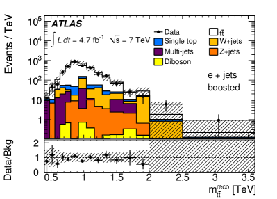
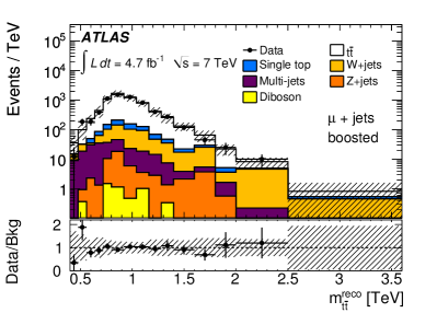
Figure 57: The reconstructed invariant mass $m_{t\bar{t}}$ measured by ATLAS in $t\bar{t}$ events (a) with an electron and using a selection based on $R=0.4$ jets (resolved), (b) with a muon and the resolved selection, (c) with an electron and using $R=1.0$ fat jets (boosted selection), (d) with a muon and using the boosted selection. The simulated $t\bar{t}$ events are from MC@NLO. The $W\!$+jets events are generated with ALPGEN+HERWIG. The multijet contribution is determined from data. From [127].

The $m_{t\bar{t}}$ spectrum for electron and muon events is shown in Figure 57 for the resolved and the boosted selection. Note that events which pass the boosted selection are not considered for the resolved selection. However, even at high reconstructed invariant masses, the resolved selection has more events. This is due to the bad mass resolution of the resolved selection which smears events from low true invariant masses to high reconstructed $m_{t\bar{t}}$.

No deviation from the SM expectation is observed and limits are set on the production cross section times branching ratio into $t\bar{t}$ for two benchmark models of New Physics. The first is a leptophobic $Z^{\prime}$ boson which is predicted by technicolor models [32, 33, 135]. Model IV of [33] is used, with $f_{1}=1$, $f_{2}=0$, and the corrections to the Lagrangian discussed in [135] are included. The couplings of this new hypothetical particle are such that the width is small in comparison to the mass, $\Gamma_{Z^{\prime}}/m_{Z^{\prime}}=1.2\%$. This width is also smaller than the detector $m_{t\bar{t}}$ resolution of $\approx\!10\%$. The second benchmark is a Kaluza-Klein gluon ($g_{\rm KK}$) that is predicted by a Randall-Sundrum model of warped extra-dimensions [41, 136, 137, 138, 139]. The width of this particle is $\Gamma_{g_{\rm KK}}/m_{g_{\rm KK}}=15.3\%$.

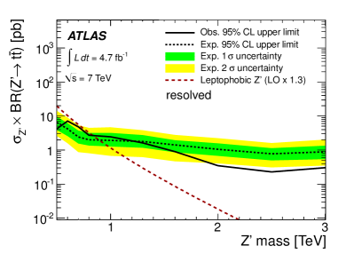
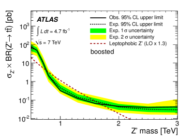
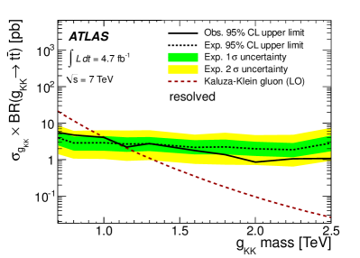
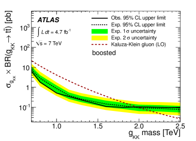
Figure 58: The $95\%$ credibility level upper limit on the production cross section times branching ratio into $t\bar{t}$ for a leptophobic $Z^{\prime}$ boson with width $\Gamma_{Z^{\prime}}/m_{Z^{\prime}}=1.2\%$ using (a) the resolved selection and (b) the boosted selection and for a Kaluza-Klein gluon with width $\Gamma_{g_{\rm KK}}/m_{g_{\rm KK}}=15.3\%$ using (c) the resolved selection and (d) the boosted selection. Events that pass the boosted selection are not considered for the resolved selection. The limits are obtained from an analysis of semileptonic $t\bar{t}$ decays. The expected limit is obtained by using background-only pseudo-experiments. From [127].

To illustrate the impact of the substructure technique, the limits obtained using either only the resolved selection or only the boosted selection are shown in Figure 58 where the electron and muon channels have been combined. The expected limit from the boosted selection is better than that from the resolved selection for masses larger than $0.8{\mathrm{\ Te\kern-1.00006ptV}}$. The better limit is a result of the better mass resolution of the boosted selection.

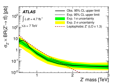
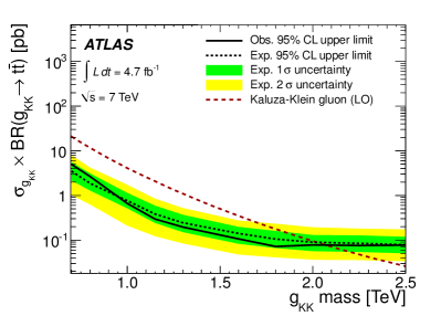
Figure 59: The $95\%$ credibility level upper limit on the production cross section times branching ratio into $t\bar{t}$ for (a) a leptophobic $Z^{\prime}$ boson with width $\Gamma_{Z^{\prime}}/m_{Z^{\prime}}=1.2\%$ and (b) a Kaluza-Klein gluon with width $\Gamma_{g_{\rm KK}}/m_{g_{\rm KK}}=15.3\%$. The limits are obtained from an analysis of semileptonic $t\bar{t}$ decays. From [127].

The limit obtained when combining the electron and muon events and both the resolved and the boosted selection is shown in Figure 59a for the $Z^{\prime}$ boson. Such a particle is excluded to have a mass between $0.5$ and $1.74{\mathrm{\ Te\kern-1.00006ptV}}$ at $95\%$ credibility level (C.L.). The limit on the Kaluza-Klein gluon is shown in Figure 59b and excludes masses $0.7<m_{g_{\rm KK}}<2.07{\mathrm{\ Te\kern-1.00006ptV}}$. No double counting occurs: the boosted and resolved selection are orthogonal because only events which fail the boosted selection are considered for the resolved selection. Also the electron/muon channels are orthogonal. The final limit setting procedure uses all four $m_{t\bar{t}}$ spectra of Figure 57 separately, i.e., the histograms are not added for the combined limit. Adding the histograms would spoil the high mass limit because the smearing from low true to high reconstructed $m_{t\bar{t}}$ in the resolved selection buries the high mass signal.

Using the data from 2011, the CMS finds limits that are less stringent than those from ATLAS: the $Z^{\prime}$ boson is excluded by CMS for masses between $0.5$ and $1.49{\mathrm{\ Te\kern-1.00006ptV}}$ and the KK gluon in the mass range $1.00$–$1.82{\mathrm{\ Te\kern-1.00006ptV}}$ [140].

10.2 $t\bar{t}$ resonances in the hadronic decay channel

Both ATLAS and CMS have published analyses that use the hadronic decay channel to search for $t\bar{t}$ resonances. The analyses use different approaches to top tagging and background estimation.

10.2.1 ATLAS HEPTopTagger analysis

ATLAS has analysed $4.7$ fb^-1 of $\sqrt{s}=7{\mathrm{\ Te\kern-1.00006ptV}}$ data [117] using both the Top Template Tagger and the HEPTopTagger. The ATLAS HEPTopTagger analysis is described in detail in [142]. Events are triggered by requiring a large sum of jet $E_{\rm T}$ in the event or several jets with low $E_{\rm T}$. At the analysis level, each event has to contain at least two $\mathrm{C/A}$ $R=1.5$ fat jets with $p_{\rm T}>200{\mathrm{\ Ge\kern-1.00006ptV}}$ and $|\eta|<2.5$. Each fat jet serves as input to the HEPTopTagger and top quark candidates with $p_{\rm T}>200{\mathrm{\ Ge\kern-1.00006ptV}}$ are kept. The two leading $p_{\rm T}$ candidates are used to calculate the invariant mass $m_{t\bar{t}}$.

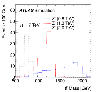
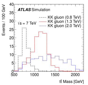
Figure 60: The HEPTopTagger reconstructed invariant mass $m_{t\bar{t}}$ using simulated ATLAS events with decays $X\rightarrow t\bar{t}\rightarrow bqq\,bqq$ for (a) $X=Z^{\prime}$ (from PYTHIA) and (b) $X=g_{\rm KK}$ (from MadGraph+PYTHIA). The production cross sections times branching ratios into $t\bar{t}$ are set to $1$ pb and the luminosity corresponds to $4.7\leavevmode\nobreak\ {\rm fb}^{-1}$. From [117].

Figure 60 shows the $m_{t\bar{t}}$ spectrum for simulated events with decays of $Z^{\prime}$ bosons and Kaluza-Klein gluons of different masses. The $m_{t\bar{t}}$ resolution is better than in the lepton+jets analysis (Figure 55). For a $g_{\rm KK}$ of mass $1.3{\mathrm{\ Te\kern-1.00006ptV}}$, the boosted lepton+jets distribution has a full width at half maximum of $500{\mathrm{\ Ge\kern-1.00006ptV}}$ whereas with the HEPTopTagger the width is $400{\mathrm{\ Ge\kern-1.00006ptV}}$. For a $Z^{\prime}$ boson of the same mass the widths are $400{\mathrm{\ Ge\kern-1.00006ptV}}$ and $200{\mathrm{\ Ge\kern-1.00006ptV}}$, respectively. For a $Z^{\prime}$ of mass $2{\mathrm{\ Te\kern-1.00006ptV}}$ the two widths are equal ($600{\mathrm{\ Ge\kern-1.00006ptV}}$). These widths are dominated by detector resolution; the natural widths are $1.2\%$ and $15.3\%$ for the $Z^{\prime}$ boson and the KK gluon, respectively.

Background from multijet events is reduced by requiring a $b$-tag in the vicinity of each fat jet. A tagged anti-$k_{\rm T}$ $R=0.4$ $b$-jet must lie within $\Delta R_{\eta}=1.4$ of each fat jet axis.

The efficiency to select events from $Z^{\prime}$ boson or $g_{\rm KK}$ decay depends on the $p_{\rm T}$ of the top and bottom quarks and is less than $6\%$ for masses of the new particles between $0.5$ and $2{\mathrm{\ Te\kern-1.00006ptV}}$. Compared to the boosted selection in muon+jets events (cf. Section 10.1), the efficiency is similar for masses below $1.3{\mathrm{\ Te\kern-1.00006ptV}}$ and smaller for larger masses.

	$1$ top tag	$\geq 2$ top tags
no $b$-tag	U (0.3%)	V (2.4%)
1 $b$-tag	W (3.2%)	X (24.3%)
$\geq 2$ $b$-tags	Y (22.5%)	Z (80.9%)

Table 2: Regions used to validate the simulation and estimate the background in the HEPTopTagger analysis. The values in parentheses are SM $t\bar{t}$ purities determined from simulation. From [117].

Control regions are defined by loosening the requirements on the number of tagged top and bottom quarks as specified in Table 2. These regions are used to validate the simulation and estimate the background. The dominating SM process ($80.9\%$) is $t\bar{t}$ production and its contribution to the $m_{t\bar{t}}$ spectrum is determined from simulation. The simulation is validated in region Y, which contains exactly one top tag, by comparing the measured top quark candidate mass distribution with that predicted by the $t\bar{t}$ simulation and a background template taken as the data distribution in region W (after subtracting a small $t\bar{t}$ contribution). The background is dominated by multijet events and the shape of the reconstructed fake top mass is significantly different from that of reconstructed top quarks. A fit to the data is performed to determine the normalisations of the background and $t\bar{t}$ distributions as shown in Figure 61. The fitted sum describes the data distribution very well. The normalisation obtained in this way for the $t\bar{t}$ simulation corresponds to the predicted normalisation within a statistical fit uncertainty of $9\%$. This result is used to constrain the $t\bar{t}$ normalisation in the analysis.

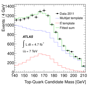
Figure 61: The distribution of the HEPTopTagger top quark candidate mass as measured in control region Y. Also shown are the contributions from $t\bar{t}$ simulation (MC@NLO) and the template from region W, the normalisations of which have been fitted such that the sum describes the data. From [117].

The rest of the SM contribution (mostly multijet events) is determined from data by extrapolating from sideband regions. For multijet events, the number of $b$-tags and the number of top tags are uncorrelated to first order because the HEPTopTagger does not use $b$-tagging information internally. A small correlation is however present because the bottom and top tagging fake rates both increase with the $p_{\rm T}$ of the jet under study (anti-$k_{\rm T}$ $R=0.4$ and $\mathrm{C/A}$ $R=1.5$, respectively). For the $b$-jets, this was shown in Figure 20b. The HEPTopTagger fake rate dependence on the fat jet $p_{\rm T}$ is displayed in Figure 46c. Multijet events with a $b$-tag have, on average, larger $b$-jet $p_{\rm T}$ and, because of the vicinity matching between the $b$-jet and the fat jet, this implies larger fat jet $p_{\rm T}$. The top quark fake rate is therefore larger in $b$-tagged multijet events. The analysis could be made insensitive to this correlation by applying the background estimation in bins of fat jet $p_{\rm T}$ (or in bins of $m_{t\bar{t}}$ because high invariant masses are reached in multijet events only if the fake top candidates are back-to-back). This has not been done in [117].

In [117], the background distribution as a function of a variable $x$ (e.g., fat jet $p_{\rm T}$, top quark candidate $p_{\rm T}$, $m_{t\bar{t}}$) in the signal region Z is determined from the average of the distributions in regions V and X, normalised to the ratio of the event count in region Y to that in U and W, respectively:

$$\frac{\text{d}n_{Z}}{\text{d}x}=\frac{1}{2}\left(\frac{n_{Y}}{n_{U}}\,\frac{\text{d}n_{V}}{\text{d}x}+\frac{n_{Y}}{n_{W}}\,\frac{\text{d}n_{X}}{\text{d}x}\right)\,,$$ (37)

with half the difference between the two averaged estimates serving as a relative systematic uncertainty of $14\%$ [142]. The simulated $t\bar{t}$ contribution has been subtracted from all regions in (37). The shape of the spectrum of $x$ is taken from regions V and X which both contain two top quark candidates so that the procedure is applicable to $m_{t\bar{t}}$ without kinematic corrections which are necessary for the CMS analysis described below (Section 10.2.3). The correlation between $b$-tags and top tags implies that the distributions of the fat jet $p_{\rm T}$, the top quark candidate $p_{\rm T}$, and $m_{t\bar{t}}$ are different in region Z than in X and V because more $b$-tags imply larger $p_{\rm T}$.

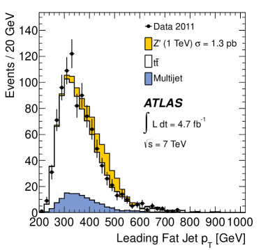
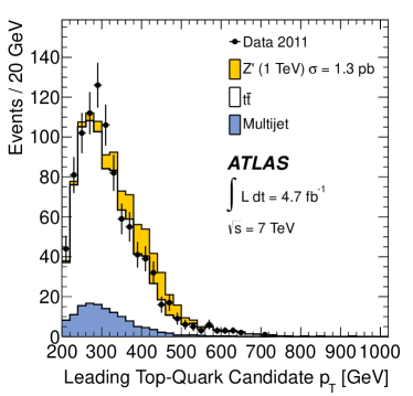
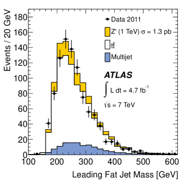
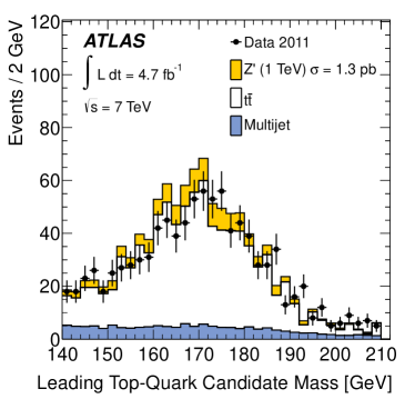
Figure 62: Control distributions of (a) the leading fat jet $p_{\rm T}$, (b) the leading top quark candidate $p_{\rm T}$, (c) the leading $p_{\rm T}$ fat jet mass, and (d) the leading $p_{\rm T}$ top quark candidate mass in the HEPTopTagger analysis of hadronically decaying $t\bar{t}$ pairs. Also shown are contributions from the prediction of SM $t\bar{t}$ production from simulation (MC@NLO), from the data-driven estimate of the remaining SM contributions (Multijet), and from a hypothetical $Z^{\prime}$ boson (from PYTHIA). From [117].

Control plots in the signal region Z of the $p_{\rm T}$ and mass of the leading $p_{\rm T}$ fat jet and the top quark candidate are shown in Figure 62. Also shown are the contributions of SM $t\bar{t}$ production and the non-top background estimate. If the correlation between $b$-tags and top tags had a significant impact on the background estimation, this would show up in the $p_{\rm T}$ distributions. Both the $p_{\rm T}$ and the mass distributions are well described in shape and normalisation by the SM predictions within the statistical uncertainties of the data. The impact of the correlation effect therefore has to be smaller than those uncertainties. Also indicated is the contribution from a $Z^{\prime}$ boson which leads to a clear overestimation of the data in the leading top quark candidate $p_{\rm T}$ distribution between $340$ and $540{\mathrm{\ Ge\kern-1.00006ptV}}$ and the leading fat jet $p_{\rm T}$ between $420$ and $520{\mathrm{\ Ge\kern-1.00006ptV}}$.

The largest systematic uncertainties result from the imperfect knowledge of the $b$-tagging efficiency ($19\%$ on the $t\bar{t}$ event yield) and the $t\bar{t}$ cross section ($12\%$) [142]. The energy scale of the HEPTopTagger subjets contributes only $8\%$ to the total relative uncertainty.

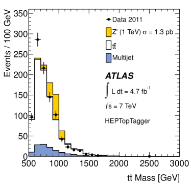
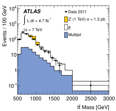
Figure 63: The HEPTopTagger reconstructed invariant mass $m_{t\bar{t}}$ (a) on a linear vertical scale and (b) on a logarithmic scale. Also shown are contributions from the prediction of SM $t\bar{t}$ production from simulation (MC@NLO), from the data-driven estimate of the remaining SM contributions (Multijet), and from a hypothetical $Z^{\prime}$ boson (from PYTHIA). From [117].

The $m_{t\bar{t}}$ spectrum is shown in Figure 63. No deviation from the SM expectation is observed and limits are set on the production cross section times branching ratio into $t\bar{t}$ for the $Z^{\prime}$ bosons and Kaluza-Klein gluon benchmark models described in Section 10.1. The limits are shown in Figure 64 and exclude the $Z^{\prime}$ boson with masses $0.70<m_{Z^{\prime}}<1.00{\mathrm{\ Te\kern-1.00006ptV}}$ and $1.28<m_{Z^{\prime}}<1.32{\mathrm{\ Te\kern-1.00006ptV}}$ and the Kaluza-Klein gluon for $0.70<m_{g_{\rm KK}}<1.48{\mathrm{\ Te\kern-1.00006ptV}}$ at $95\%$ C.L. The limits are less stringent than in the lepton+jets case. For low masses, the resolved selection of the lepton analysis has a higher selection efficiency than the HEPTopTagger selection. Compared to the boosted muon selection, the HEPTopTagger analysis suffers mainly from an efficiency decrease at high $p_{\rm T}$ due to the additional required $b$-tag.

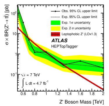
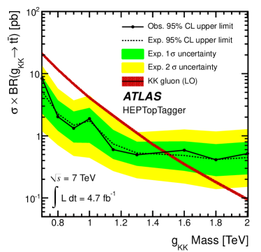
Figure 64: The $95\%$ credibility level upper limit on the production cross section times branching ratio into $t\bar{t}$ for (a) a leptophobic $Z^{\prime}$ boson with width $\Gamma_{Z^{\prime}}/m_{Z^{\prime}}=1.2\%$ and (b) a Kaluza-Klein gluon with width $\Gamma_{g_{\rm KK}}/m_{g_{\rm KK}}=15.3\%$. The limits are obtained from a HEPTopTagger analysis of hadronic $t\bar{t}$ decays. From [117].

10.2.2 ATLAS Top Template Tagger analysis

ATLAS used the same data set that was used for the lepton+jets (Section 10.1) and HEPTopTagger analyses (Section 10.2.1) also for an analysis that employed the Top Template Tagger. For every top quark $p_{\rm T}$ bin of width $100{\mathrm{\ Ge\kern-1.00006ptV}}$, starting from $450{\mathrm{\ Ge\kern-1.00006ptV}}$, $300,\!000$ templates of parton configurations were calculated and stored. These numbers were optimised for maximal top quark tagging efficiency at high background rejection.

The events are triggered by an anti-$k_{\rm T}$ $R=1.0$ fat jet with $E_{\rm T}>240{\mathrm{\ Ge\kern-1.00006ptV}}$ and are required to have at least two anti-$k_{\rm T}$ $R=1.0$ fat jets with $|\eta|<2$. The leading $p_{\rm T}$ jet is required to have $p_{\rm T}>500{\mathrm{\ Ge\kern-1.00006ptV}}$ and the subleading jet $p_{\rm T}>450{\mathrm{\ Ge\kern-1.00006ptV}}$. These two fat jets must be tagged by the Top Template Tagger algorithm. Each fat jet must have a $b$-tagged anti-$k_{\rm T}$ $R=0.4$ jet within $\Delta R_{\eta}=1.0$ of the fat jet axis.

The efficiency for selecting events from decays of high mass $Z^{\prime}$ bosons is higher than for the HEPTopTagger analysis: $8\%$ for $m_{Z^{\prime}}=1.6{\mathrm{\ Te\kern-1.00006ptV}}$, and $6\%$ for $1.3$ and $2.0{\mathrm{\ Te\kern-1.00006ptV}}$. The reason for the higher efficiency is a better top quark finding efficiency when using the Top Template Tagger (the same number of $b$-tags are required in the two analyses). The Top Template Tagger efficiency is $75(5)\%$ for the leading $p_{\rm T}$ fat jet and $62(5)\%$ for the subleading fat jet, which are both larger than the plateau efficiency of the HEPTopTagger ($\approx\!40\%$). For masses below $1{\mathrm{\ Te\kern-1.00006ptV}}$, the selection efficiency is an order of magnitude smaller than in the HEPTopTagger analysis because of the larger required fat jet $p_{\rm T}$ ($500{\mathrm{\ Ge\kern-1.00006ptV}}$ vs. $200{\mathrm{\ Ge\kern-1.00006ptV}}$).

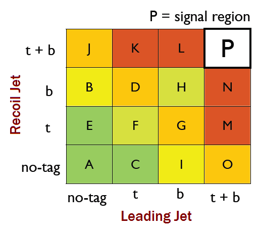
Figure 65: Subsamples used to determine the non-$t\bar{t}$ background in the Top Template Tagger ATLAS analysis of hadronic $t\bar{t}$ decays. The division is by bottom and top tagging states of the leading $p_{\rm T}$ and subleading $p_{\rm T}$ (Recoil Jet) fat jets. From [117].

The SM $t\bar{t}$ background is determined from simulation. The remaining SM contribution is determined using a sideband extrapolation method based on the bottom and top tagging states of the leading and subleading $p_{\rm T}$ fat jets. The data are divided into 16 subsamples as shown in Figure 65. The top tagging fake rates for the leading and subleading $p_{\rm T}$ fat jet in multijets events are correlated because the transverse momenta of the two fat jets are correlated: the events are dominated by hard $2\to 2$ parton scattering with equal $p_{\rm T}$ in the centre-of-mass system of the hard scatter. A simple extrapolation using regions A, O, and J to estimate the event count in P is therefore not possible. Instead, the method relies on the assumption that the $b$-tagging and top tagging fake rates are independent. This assumption is only approximately valid because both rates depend on $p_{\rm T}$ as discussed in Section 10.2.1. The regions K, L, M, and N can contain sizeable contributions from physics beyond the standard model and are not used directly. Instead, the event counts in K and N are estimated from regions with smaller contamination and these estimates are then used to predict the count in region P:

$$N_{K^{\prime}} = N_{J}\times N_{F}/N_{E}\,,$$ (38)

$$N_{M^{\prime}} = N_{F}\times N_{O}/N_{C}\,,$$ (39)

$$N_{P} = N_{K^{\prime}}\times N_{M^{\prime}}/N_{F}\,.$$ (40)

A direct comparison of the control regions with those in the HEPTopTagger analysis is not possible because the latter made use of all fat jets in the event and not just the two leading $p_{\rm T}$ ones. The HEPTopTagger control region U corresponds to regions C and E, and region W to D and G. Region V includes region F, region X includes regions K and M, and region Y includes L and N. It is interesting that K, L, M, N could not be used directly in the Top Template Tagger analysis because of signal contamination while no such problem was observed in the HEPTopTagger analysis. This could be explained if the correlation with $b$-tagging is different for the two top finding algorithms.

Other combinations of control regions are used in the Top Template Tagger analysis to estimate a systematic uncertainty on the non-$t\bar{t}$ background. The dominating systematic uncertainties in the analysis are from $b$-tagging, the fat jet energy scale, and the SM $t\bar{t}$ normalisation.

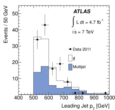
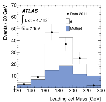
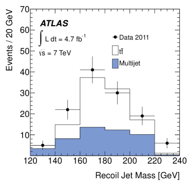
Figure 66: Distributions of (a) the leading fat jet $p_{\rm T}$, (b) the leading $p_{\rm T}$ fat jet mass, (c) the subleading fat jet $p_{\rm T}$, and (d) the subleading $p_{\rm T}$ fat jet mass in the Top Template Tagger analysis of hadronically decaying $t\bar{t}$ pairs. Also shown are contributions from the prediction of SM $t\bar{t}$ production from simulation (MC@NLO), and from the data-driven estimate of the remaining SM contributions (Multijet). From [117].

Control plots of the $p_{\rm T}$ and mass of the two tagged fat jets are shown in Figure 66. The statistical uncertainties of the data are large because of the high fat jet $p_{\rm T}$. For high leading $p_{\rm T}$ fat jet mass the estimated multijet contribution overestimates the data significantly whereas in all other bins it is compatible with the data within the statistical data uncertainty. The ratio of $t\bar{t}$ to multijet events in the fat jet $p_{\rm T}$ spectrum is $\approx\!1$ which has to be compared to a ratio of $\approx\!4$ in the HEPTopTagger analysis which also holds for fat jet $p_{\rm T}>500{\mathrm{\ Ge\kern-1.00006ptV}}$. In [117], the Top Template Tagger mis-tag rate for a light quark or gluon fat jet is quoted to be $\approx\!10\%$. The corresponding HEPTopTagger fake rate is $2.5\%$ [106, 102].

The invariant mass spectrum $m_{t\bar{t}}$ is shown in Figure 67a. No excess of events over the SM contributions is observed and limits are set. No exclusion limits can be set on the masses of the narrow width $Z^{\prime}$ boson benchmark model as shown in Figure 67b. For the Kaluza-Klein gluon model the excluded masses are $1.02<m_{g_{\rm KK}}<1.62$ at $95\%$ C.L. (Figure 67c). The upper limit is better than the one from the HEPTopTagger due to the higher analysis efficiency at high mass. The lower mass limit is significantly less stringent than that from the HEPTopTagger.

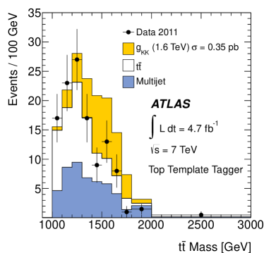
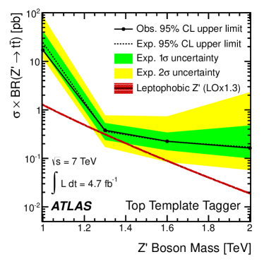
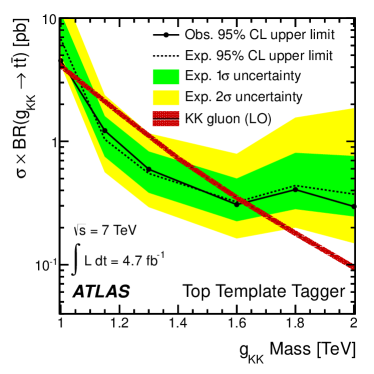
Figure 67: (a) The invariant mass $m_{t\bar{t}}$ reconstructed with the Top Template Tagger. Also shown are contributions from the prediction of SM $t\bar{t}$ production from simulation (MC@NLO), from the data-driven estimate of the remaining SM contributions (Multijet), and from a hypothetical Kaluza-Klein gluon (from PYTHIA). The $95\%$ credibility level upper limit on the production cross section times branching ratio into $t\bar{t}$ for (b) a leptophobic $Z^{\prime}$ boson with width $\Gamma_{Z^{\prime}}/m_{Z^{\prime}}=1.2\%$ and (c) a Kaluza-Klein gluon with width $\Gamma_{g_{\rm KK}}/m_{g_{\rm KK}}=15.3\%$. From [117].

10.2.3 CMS Top Tagger analysis

A search for hadronically decaying $t\bar{t}$ resonances was published by CMS in [122] using $5\leavevmode\nobreak\ {\rm fb}^{-1}$ of data collected at $\sqrt{s}=7{\mathrm{\ Te\kern-1.00006ptV}}$. Events are triggered by requiring a jet with $p_{\rm T}>300{\mathrm{\ Ge\kern-1.00006ptV}}$ ($240{\mathrm{\ Ge\kern-1.00006ptV}}$ in early 2011 running conditions). Fat jets are selected offline using the $\mathrm{C/A}$ algorithm with $R=0.8$. The detector volume is divided into two hemispheres, corresponding to positive and negative pseudorapidities, respectively. The fat jet multiplicities in the two hemispheres are used to classify the events into two categories: the ‘1+1’ channel with one fat jet in either hemisphere and the ‘1+2’ channel for which one hemisphere has at least two fat jets.

The fat jets in single-fat-jet hemispheres must be tagged by the CMS Top Tagger algorithm discussed in Section 7.6. The top quark candidate $p_{\rm T}$ is required to be larger than $350{\mathrm{\ Ge\kern-1.00006ptV}}$.

One of the fat jets that share a hemisphere in 1+2 events must be tagged as coming from hadronic $W$ boson decay. The $W$ boson tag requires the pruned jet mass to be between $60$ and $100{\mathrm{\ Ge\kern-1.00006ptV}}$ (the pruning parameters $z_{\rm cut}$ and $D_{\rm cut}$ are presumably chosen to correspond to the values in the original publication [59] which are given in Section 3.4) and two subjets with a mass drop of at least $60\%$. The fat jet closest to the $W$ boson candidate jet in $(\eta,\phi)$ space is taken to be the $b$-jet (although no $b$-tagging algorithm is used). The combination of the four-momenta of these two fat jets has to yield a mass in the range $140$ to $250{\mathrm{\ Ge\kern-1.00006ptV}}$ ($W\!\!+\!b$ tag).

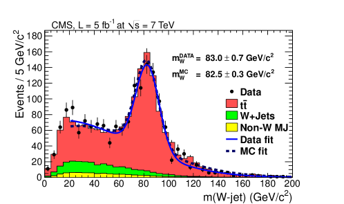
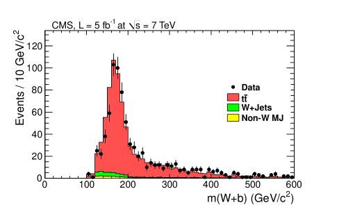
Figure 68: (a) The mass of the leading mass $W$ boson candidate pruned fat jet in the hemisphere opposite to that of the muon in semileptonic $t\bar{t}$ events. (b) The invariant mass of the combination of the $W$ boson candidate fat jet and the closest fat jet. Also shown are simulated events from SM $t\bar{t}$ production (MadGraph+PYTHIA). The multijet distribution is obtained from data by reversing the muon isolation criteria. The $W\!$+jets shape is assumed to be identical to the multijet shape and the normalisation is obtained from the inclusive $W$ boson production cross section. From [122].

The extend to which the selection is modelled in simulation is tested using an event sample of semileptonic $t\bar{t}$ decays with a single final state muon and at least one $b$-tag. The limited number of events does not permit the validation of the simulated top tagging efficiency. This would require significantly large numbers of fat jets with high $p_{\rm T}$ to capture all top quark decay products. Instead, the simulated jet energy scale and the selection efficiency was validated for the $W\!\!+\!b$ tag. Figure 68a shows the distribution of the leading $W\!$-tagged fat jet mass in the hemisphere opposite the one containing the muon. A clear peak is visible near the $W$ boson mass. The jet mass is given by the invariant mass of the two subjets and the peak position therefore reflects the subjet energy scale. The peak position is extracted through a fit and the position in simulation agrees with that in data within $1\%$ which corresponds to the statistical uncertainties of the fits. The $W$ tag selection efficiency is determined by comparing the number of events in the mass window from $60$ to $100{\mathrm{\ Ge\kern-1.00006ptV}}$ in Figure 68a with the number of all events in the semileptonic $t\bar{t}$ sample. The efficiencies for data and simulation are $49\%$ and $50\%$, respectively, with relative uncertainties of $2\%$. The mass drop efficiency is determined in a similar way ($64\%$) and the overall simulated efficiency overestimates the efficiency by $3\%\pm 3\%$.

The mass of the combination of the $W$ boson candidate and the closest fat jet in semileptonic $t\bar{t}$ events is shown in Figure 68b. A clear peak is visible near the top quark mass with a tail to larger masses. The position of the peak is approximately described by the simulation (mostly SM $t\bar{t}$ production), although the prediction seems shifted to lower values by $\approx\!10{\mathrm{\ Ge\kern-1.00006ptV}}$. This shift corresponds to $6\%$ at the top quark mass, much more than the $1\%$ uncertainty that was extracted from the description of the $W$ boson mass peak. The larger discrepancy for the top quark mass peak could be related to the fact that the $b$-jet in $t\to bqq$ decay has on average the largest $p_{\rm T}$ of all decay quark jets (see for example Figure 44a and its discussion). The uncertainty on the simulation of the higher $p_{\rm T}$ subjets therefore seems to be larger than that for the lower $p_{\rm T}$ subjets from $W$ boson decay. Using only the $W$ boson mass peak to determine the subjet energy scale uncertainty is therefore not recommended because it does not sample the full phase space relevant to a top quark analysis.

A data control region is used to determine the fake top tagging rate for the multijets background. The control region is defined by selecting 1+2 events in which the $W$ boson candidate and the $W\!\!+\!b$ candidate satisfy the mass window requirements to make the selection kinematically similar to the signal region but the mass drop requirement on the $W$ candidate is inverted to remove signal-like events. The events in this control region are then used to study the tagging of the fat jet in the hemisphere opposite the $W\!\!+\!b$ candidate. The fake top tagging rate is shown in Figure 69. It is approximately $0.1\%$ at the threshold and plateaus at $6\%$ for $p_{\rm T}>600{\mathrm{\ Ge\kern-1.00006ptV}}$. The rise in the mis-tag rate is due to increased QCD radiation at large $p_{\rm T}$ which can fake the top quark decay pattern. The top quark tagging efficiency is also shown. It is $8\%$ at fat jet $p_{\rm T}=350{\mathrm{\ Ge\kern-1.00006ptV}}$, rises to $20\%$ at $400{\mathrm{\ Ge\kern-1.00006ptV}}$ and reaches a plateau of $50\%$ for $p_{\rm T}>500{\mathrm{\ Ge\kern-1.00006ptV}}$. The efficiency rise is a geometric effect that results from the decay products being more collimated at large $p_{\rm T}$, eventually all being contained inside the fat jet with $R=0.8$.

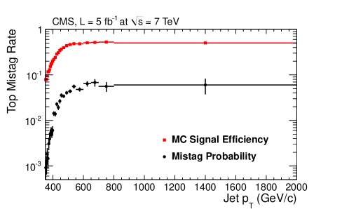
Figure 69: The CMS Top Tagger efficiency for $\mathrm{C/A}$ $R=0.8$ fat jets when no other fat jets are in the same hemisphere. Shown is the fake rate of tagging fat jets from hard light quarks or gluons determined from data and the efficiency to tag fat jets in simulated $Z^{\prime}\rightarrow t\bar{t}$ events from MadGraph (the label on the vertical axis corresponds only to the fake rate). From [122].

To determine the multijet contribution, the selection cuts are relaxed by requiring only one top tagged fat jet (loose selection). The $W\!\!+\!b$ tag is required in 1+2 events and for 1+1 events a random one of the two fat jets is required to be top tagged. These samples are dominated by multijet events. The multijet contribution remaining after the second top tag requirement is determined by weighting these events with the fake rate at the $p_{\rm T}$ of the fat jet in the hemisphere opposite to the first tag (‘probe jet’). However, the probe jets have a systematically smaller mass than those in the signal region because the majority of them are not tagged. To correct for this kinematic bias, the mass of the probe jet is ignored and replaced by a mass drawn randomly from the distribution of simulated multijet events in the range $140$ to $250{\mathrm{\ Ge\kern-1.00006ptV}}$. A systematic uncertainty is assigned by taking half the difference between the $m_{t\bar{t}}$ distributions resulting from the described procedure and when not correcting the kinematic bias.

The measured $m_{t\bar{t}}$ distributions in 1+1 and 1+2 events are shown in Figure 70. The largest SM contribution is from multijets and only $3$–$13\%$ from $t\bar{t}$ production, depending on the mass and the event class. At masses around $1{\mathrm{\ Te\kern-1.00006ptV}}$, the background uncertainty is $5\%$ and the largest systematic uncertainty is the trigger uncertainty of $13\%$ for 1+1 events and $20\%$ for 2+2 events. The trigger uncertainty is taken to be half the trigger inefficiency predicted by simulation. For masses larger than $2.5{\mathrm{\ Te\kern-1.00006ptV}}$, the biggest uncertainty results from the finite statistics of the single-tag multijets sample. No significant excess over the SM contributions is observed and limits are set.

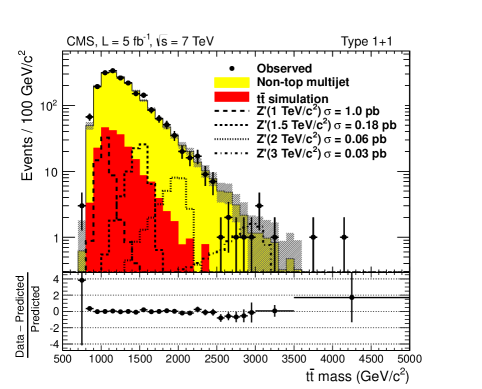
Figure 70: The reconstructed $m_{t\bar{t}}$ spectrum for (a) 1+1 events and (b) 1+2 events using the CMS Top Tagger. Also shown are SM contributions from multijet events determined from data and simulated $t\bar{t}$ production (from MadGraph+PYTHIA). The spectra from $Z^{\prime}\rightarrow t\bar{t}$ decays for several masses of a hypothetical $Z^{\prime}$ boson with width $\Gamma_{Z^{\prime}}/m_{Z^{\prime}}=1\%$ are indicated (from MadGraph). From [122].

The uncertainty on the multijet background is remarkably small. For comparison, in the ATLAS HEPTopTagger analysis, the multijet background uncertainty is $14\%$ (Section 10.2.1). ATLAS took the approach to reduce the multijet background through $b$-tag requirements. The $19\%$ relative uncertainty on the $b$-tagging simulation at high $p_{\rm T}$ is the main contributor to the total uncertainty in the ATLAS HEPTopTagger analysis. Given the small uncertainty found by CMS, it seems that foregoing the use of $b$-tagging at high $p_{\rm T}$ is the better strategy until improved $b$-tagging algorithms will be developed for that region. But since the relative background uncertainty for CMS is a factor of $\approx\!3$ smaller than the one for ATLAS, examining the origins of this small uncertainty is warranted.

As described above, the multijet contribution in the signal region is obtained by weighting fat jet pairs in a loose selection by the fake rate. In the mass ranges $0.9<m_{t\bar{t}}<1.1{\mathrm{\ Te\kern-1.00006ptV}}$ and $1.3<m_{t\bar{t}}<2.4{\mathrm{\ Te\kern-1.00006ptV}}$, the statistical error on the estimated background in the final selection is quoted to be better than $1\%$. This follows from the high statistics in the loose selection. The background uncertainty is dominated by the systematic error which is described as resulting “from the systematic uncertainty assigned to the procedure for modifying the probe-jet masses” and which is $3$–$5\%$, depending on the mass range and the event topology (1+1, 1+2) [122]. The statistical uncertainty on the fake rate is quoted to be “ranging from $<\!\!1\%$ at $1{\mathrm{\ Te\kern-1.00006ptV}}/c^{2}$ to $\approx\!\!10\%$ at $3{\mathrm{\ Te\kern-1.00006ptV}}/c^{2}$” [122]. Unfortunately, no mention is made of how the small uncertainties on the fake rate are arrived at; the error bars in Figure 69 correspond to much larger uncertainties.

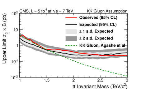
Figure 71: The $95\%$ confidence level upper limit on the production cross section times branching ratio into $t\bar{t}$ for (a) a leptophobic $Z^{\prime}$ boson with width $\Gamma_{Z^{\prime}}/m_{Z^{\prime}}=1.2\%$ and $3.0\%$ and (b) a Kaluza-Klein gluon with width $\Gamma_{g_{\rm KK}}/m_{g_{\rm KK}}=15.3\%$. From [122].

Figure 71a and b show the limits for the narrow-width $Z^{\prime}$ boson and the Kaluza-Klein gluon, respectively. Below $1{\mathrm{\ Te\kern-1.00006ptV}}$ the multijet background is prohibitively large and the selection is inefficient for the signal models. No limits are therefore evaluated for this parameter space. The limit for the $Z^{\prime}$ model is calculated assuming a width of $1.0\%$ which is much smaller than the $m_{t\bar{t}}$ detector resolution of $\approx\!10\%$. Any resonance width smaller than $10\%$ will be broadened by detector resolution. For this reason, it is possible to compare the $Z^{\prime}$ $1.2\%$ width model with the $1.0\%$ limit.

The $1.2\%$ width $Z^{\prime}$ boson model is the benchmark model also used in the ATLAS analyses (Figures 59, 64, and 67) and the cross section predictions are identical (including a scaling of the leading order prediction by a factor of $1.3$). This model can be excluded at $95\%$ confidence level at $m_{Z^{\prime}}=1{\mathrm{\ Te\kern-1.00006ptV}}$ and in the range $\approx\!1.33$–$1.46{\mathrm{\ Te\kern-1.00006ptV}}$. Compared to the HEPTopTagger analysis, the upper mass limit is $140{\mathrm{\ Ge\kern-1.00006ptV}}$ higher. The HEPTopTagger analysis, on the other hand, provides a limit for masses below $1{\mathrm{\ Te\kern-1.00006ptV}}$.

The Kaluza-Klein gluon model used by CMS has a cross section that is $\approx\!10\%$ higher at $m_{g_{\rm KK}}=1.5{\mathrm{\ Te\kern-1.00006ptV}}$ than the model used by ATLAS. The CMS exclusion limit is a small interval near $1{\mathrm{\ Te\kern-1.00006ptV}}$ and $1.42$–$1.5{\mathrm{\ Te\kern-1.00006ptV}}$. In this latter mass range, the ATLAS Kaluza-Klein gluon model cannot be excluded by the CMS analysis.

10.3 Summary of $t\bar{t}$ resonance searches

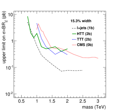
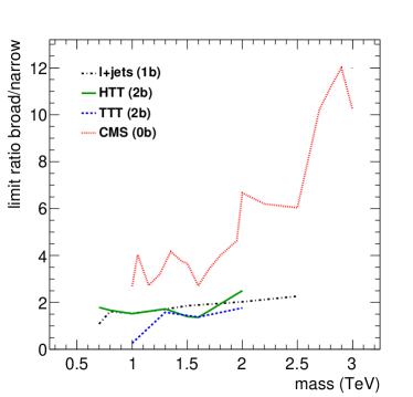
Figure 72: The observed $95\%$ C.L. upper limits on the production cross section times branching ratio into $t\bar{t}$ for (a) a narrow resonance (width $\Gamma/m=1.2\%$) for which the reconstructed width is given by the detector resolution of $\approx\!10\%$ and (b) a broader resonance of width $15.3\%$. The ratio of the limit of the broader to the narrower resonance is shown in (c). The limits are taken from the ATLAS analyses using lepton+jets [127], the hadronic ATLAS analyses [117] using the HEPTopTagger (label ‘HTT’) and the Top Template Tagger (‘TTT’), and the hadronic CMS analysis using their top tagger [122].

Figure 72 shows a comparison of the observed limits in the $t\bar{t}$ resonance searches as a function of the mass $m$ of the new particle. The limits are shown for the case of a narrow resonance ($\Gamma/m=1.2\%$), for which the reconstructed width is given by the detector resolution of $\approx\!10\%$ and a broader resonance of width $15.3\%$.

The best limits for masses between $1$ and $2.5{\mathrm{\ Te\kern-1.00006ptV}}$ are given by the semileptonic analysis. For masses larger than $1.3{\mathrm{\ Te\kern-1.00006ptV}}$ the limits are below $0.1$ pb. For the broad resonance, the semileptonic limit is approximately a factor of $3$ better than the ones from the fully hadronic analyses. Figure 72c shows the ratios of the limit for the broad resonance to the limit for the narrow resonance. For the semileptonic analysis, the narrow resonance limit is better by a factor of $1.5$ at $1{\mathrm{\ Te\kern-1.00006ptV}}$ and $2.2$ at $2.5{\mathrm{\ Te\kern-1.00006ptV}}$. The fact that the mass exclusion range is larger for the Kaluza-Klein gluon model (cf. Section 10.1) is due to the higher production cross section of that model. All analyses set better limits on the narrower resonance, except for the Top Template Tagger at $1{\mathrm{\ Te\kern-1.00006ptV}}$.

The leptonic analysis uses a cut on the splitting scale $\sqrt{d_{12}}$ to tag the hadronically decaying top quark. This method has a high efficiency and a low rejection. A larger rejection is not needed because the multijet background is inherently lower than in the other analyses due to the lepton requirement. The analysis also uses only a single $b$-tag. The tagging of bottom quarks uses settings that have been optimised at low bottom quark $p_{\rm T}$ and which may not be optimal at high $p_{\rm T}$ because of the collimated topology with close-by jets. Also the uncertainties on the $b$-tagging efficiency and fake rate is large at high $p_{\rm T}$, thereby reducing the sensitivity of the searches.

The CMS Top Tagger analysis, which does not use $b$-tagging, has the next best limit between $1.3$ and $2.5{\mathrm{\ Te\kern-1.00006ptV}}$ for the narrow resonance. For masses larger than $2.5{\mathrm{\ Te\kern-1.00006ptV}}$ is gives the best limit and reaches $0.02$ pb at $3{\mathrm{\ Te\kern-1.00006ptV}}$. The sensitivity to the broad resonance is significantly worse. The CMS tagger shows the largest dependence on the width with the limits being a factor 3 to 12 worse for the broader resonance.

The HEPTopTagger analysis limit is as good as the semileptonic limit for $700<m<800{\mathrm{\ Ge\kern-1.00006ptV}}$. Below this range, the resolved semileptonic analysis provides a better limit. Up to $1.3{\mathrm{\ Te\kern-1.00006ptV}}$ the HEPTopTagger provides the best limit of all hadronic analyses, then the Top Template Tagger provides a comparable or better limit.

It is reassuring that the different analyses give similar limits, despite the wide range of approaches for tagging top quarks and their different systematic uncertainties. The evaluation of systematic uncertainties in boosted top quark analyses is often limited by the statistics of available high $p_{\rm T}$ top quarks in data control samples. Rather than taking the statistical uncertainties as an upper limit for the systematic errors, the low $p_{\rm T}$ uncertainties are often taken if no clear trend is visible within the large statistical errors when extrapolating to high $p_{\rm T}$. High statistics datasets that will become available in the future will allow to better constrain these uncertainties.

10.4 Search for SUSY in high jet multiplicity events

In addition to the searches for $t\bar{t}$ resonances, substructure techniques have also been used to search for SUSY. The strategy of the analysis in [143] is to look for an excess of events beyond the SM prediction in a final state with at least seven anti-$k_{\rm T}$ $R=0.4$ jets (small-$R$ jets), missing energy, and no leptons. This final state is especially sensitive to a SUSY model like that used in Section 9.3, in which top squarks decay to top quarks and neutralinos. The analysis uses a conventional selection ($b$-tag stream) and a selection that requires the sum of the masses of all fat jets to be larger than two times the top quark mass.

ATLAS data collected at $\sqrt{s}=8{\mathrm{\ Te\kern-1.00006ptV}}$ are used, corresponding to a luminosity of $20.3(6)\leavevmode\nobreak\ {\rm fb}^{-1}$. Jets are built from calorimeter clusters and multijet triggers are used to select the events, requiring at least five jets with $E_{\rm T}>55{\mathrm{\ Ge\kern-1.00006ptV}}$ or at least six jets with $E_{\rm T}>45{\mathrm{\ Ge\kern-1.00006ptV}}$. Events with isolated muons or electrons with $p_{\rm T}>10{\mathrm{\ Ge\kern-1.00006ptV}}$, that are separated from the nearest jet by at least $\Delta R_{\eta}=0.4$, are vetoed. Multiple signal regions are defined, with different jet and $b$-tag multiplicities, to enhance the sensitivity to different SUSY models.

For the $b$-tag stream, the small-$R$ jets are required to have $|\eta|<2.0$. Seven signal regions are defined using jet $p_{\rm T}>50{\mathrm{\ Ge\kern-1.00006ptV}}$: six regions with exactly eight or exactly nine jets in the event, subdivided by $b$-tag multiplicity ($0$, $1$, $\geq 2$) using the MV1 algorithm. One additional signal region is formed by events with more than nine jets without a $b$-tag requirement. Another six signal regions are defined by $p_{\rm T}>80{\mathrm{\ Ge\kern-1.00006ptV}}$ and exactly seven or at least eight jets, subdivided in $b$-tag multiplicity.

For the fat jet stream, the small-$R$ jets are required to have $|\eta|<2.8$. The fat jets are not constructed from clusters but by running the anti-$k_{\rm T}$ algorithm with $R=1.0$ over small-$R$ jets with $p_{\rm T}>20{\mathrm{\ Ge\kern-1.00006ptV}}$. These fat jets are required to have $p_{\rm T}>100{\mathrm{\ Ge\kern-1.00006ptV}}$ and $|\eta|<1.5$. The scalar sum $M_{J}^{\Sigma}$ of the masses of all fat jets is required to be larger than $340$ or $420{\mathrm{\ Ge\kern-1.00006ptV}}$ for events with at least eight, nine, or ten small-$R$ jets with $p_{\rm T}>50{\mathrm{\ Ge\kern-1.00006ptV}}$, thereby giving six signal regions.

In each of the 19 signal regions, $\mbox{$/{\!\!\!\!E_{\rm T}}$}/\sqrt{H_{\rm T}}>4\sqrt{\!\!{\mathrm{\ Ge\kern-1.00006ptV}}}$ is required, in which $H_{\rm T}$ is the scalar sum of the $p_{\rm T}$ of all small-$R$ jets with $p_{\rm T}>40{\mathrm{\ Ge\kern-1.00006ptV}}$ and $|\eta|<2.8$. For multijet ATLAS events, the shape of the $\mbox{$/{\!\!\!\!E_{\rm T}}$}/\sqrt{H_{\rm T}}$ distribution is found to be approximately independent of the small-$R$ jet multiplicity $N_{\rm jet}$ and of $M_{J}^{\Sigma}$. The multijet background in the signal regions can therefore be determined using $\mbox{$/{\!\!\!\!E_{\rm T}}$}/\sqrt{H_{\rm T}}$ templates from multijet-dominated control regions at lower $N_{\rm jet}$. The multijet background template is taken from $N_{\rm jet}=6$ events and the other backgrounds are subtracted from the template. Separate templates are used for the different $b$-tag multiplicities because neutrinos from heavy quark decay contribute to $/{\!\!\!\!E_{\rm T}}$ but not to $H_{\rm T}$. A correction is applied to account for small changes in the ratio that result from non-jet contributions to $/{\!\!\!\!E_{\rm T}}$ which do not appear in $H_{\rm T}$. The correction amounts to reweighting the distribution of non-jet $p_{\rm T}$ in the control region to that in the signal region. The closure of this method is tested for intervals at smaller $\mbox{$/{\!\!\!\!E_{\rm T}}$}/\sqrt{H_{\rm T}}$ than in the signal regions and observed deviations are used as systematic uncertainties. The closure uncertainties typically are $5$ to $15\%$, reaching up to $\approx\!50\%$ in control regions with small statistics. Figure 73 shows the $\mbox{$/{\!\!\!\!E_{\rm T}}$}/\sqrt{H_{\rm T}}$ distribution in control regions with (a) $N_{\rm jet}=7$ for the selection with at least two $b$-tags and (b) the requirement $M_{J}^{\Sigma}>340{\mathrm{\ Ge\kern-1.00006ptV}}$. The data are well described for $\mbox{$/{\!\!\!\!E_{\rm T}}$}/\sqrt{H_{\rm T}}<4\sqrt{\!\!{\mathrm{\ Ge\kern-1.00006ptV}}}$, where multijet events dominate. The closure uncertainties are determined in this region. The leptonic $t\bar{t}$ background becomes important at higher values where deviations from the data are seen in some bins. The $t\bar{t}$ background carries an uncertainty of $\approx\!50\%$ when combining experimental and theoretical sources as discussed below. Within this uncertainty, the description is compatible with the data. The control regions can potentially be contaminated with New Physics events, as illustrated in the figure. A simplified SUSY model is used with pair-produced gluinos, each decaying to $t\bar{t}\tilde{\chi}^{0}_{1}$, as introduced in Section 9.3. The masses chosen for the contributions in the figure are $m(\tilde{g})=900{\mathrm{\ Ge\kern-1.00006ptV}}$ and $m(\tilde{\chi}^{0}_{1})=150{\mathrm{\ Ge\kern-1.00006ptV}}$, which are excluded by the analysis of the signal regions as discussed below. The possible contamination is therefore smaller than that shown in Figure 73 ($20$–$30$ events per $4\sqrt{\!\!{\mathrm{\ Ge\kern-1.00006ptV}}}$).

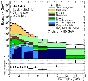
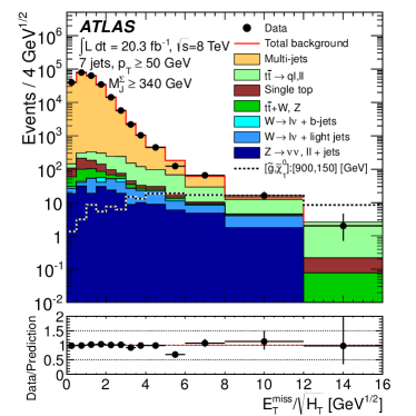
Figure 73: The $\mbox{$/{\!\!\!\!E_{\rm T}}$}/\sqrt{H_{\rm T}}$ distribution in control regions with exactly seven anti-$k_{\rm T}$ $R=0.4$ jets with $p_{\rm T}>50{\mathrm{\ Ge\kern-1.00006ptV}}$. The multijet prediction is taken from the measured distribution with exactly six jets and after subtracting the simulated leptonic backgrounds. The $t\bar{t}$ and $W\!$+jets backgrounds are generated with SHERPA and normalised in control regions. Single-top production is generated with MC@NLO in the $s$-channel and with AcerMC in the $t$-channel. Also shown is the distribution of a SUSY model with $m(\tilde{g})=900{\mathrm{\ Ge\kern-1.00006ptV}}$ and $m(\tilde{\chi}^{0}_{1})=150{\mathrm{\ Ge\kern-1.00006ptV}}$, generated with MadGraph+HERWIG++. The distribution is shown after requiring (a) at least two $b$-tags and (b) the sum of the masses of anti-$k_{\rm T}$ $R=1.0$ jets in the event to exceed $340{\mathrm{\ Ge\kern-1.00006ptV}}$. From [143].

The most important leptonic backgrounds are from $W\!$+jets events and $t\bar{t}$ production and the dominant contributions result from decays to $\tau$ leptons which decay hadronically. The decays to electrons and muons are suppressed because of the electron and muon vetos. These backgrounds are taken from SHERPA simulations which are fitted to data in control regions. The control regions contain exactly one isolated muon or electron and the lepton four-momentum is used to create an additional jet that is included in the calculation of $H_{\rm T}$. In this way, $\mbox{$/{\!\!\!\!E_{\rm T}}$}/\sqrt{H_{\rm T}}$ is made similar to its value in events with hadronic $\tau$ decay. A simultaneous fit is performed to the signal and control regions, as discussed below, to determine the SM contribution and potential contributions from New Physics.

The normalisation of the background simulation for events with $Z\rightarrow\nu\nu$ decay is taken from data using events with same-flavour, opposite-charge lepton pairs (electrons or muons) which combine to an invariant mass close to the $Z$ boson mass ($80$ to $100{\mathrm{\ Ge\kern-1.00006ptV}}$). The two transverse lepton momenta are added to $/{\!\!\!\!E_{\rm T}}$ and the prediction in the region $\mbox{$/{\!\!\!\!E_{\rm T}}$}/\sqrt{H_{\rm T}}>4\sqrt{\!\!{\mathrm{\ Ge\kern-1.00006ptV}}}$ is normalised to the data in control regions that have relaxed $N_{\rm jet}$ requirements. The same normalisation factor is then used in the signal region. Experimental systematic uncertainties are dominated by the modelling of the jet energy scale and resolution which change the event yield by $20$ to $30\%$. Smaller uncertainties of $\approx\!10\%$ result from $b$-tagging. For the $W\!$+jets events, the theoretical uncertainties are smaller than the experimental ones. For $t\bar{t}$ production, two theoretical contributions each give rise to an uncertainty of $25$–$30\%$: i) variations of the renormalisation and factorisation scales by factors $2$ and $0.5$ and ii) variations of the gluon fusion production cross section. To account for higher order terms not included in SHERPA, the probability for events to be initiated by gluon fusion is increased by $37\%$ while the other processes are reduced by a common factor to keep the total cross section unchanged. This procedure improves the description of the data in the control regions. The difference in the event yield before and after the $37\%$ correction is used as a systematic uncertainty.

Fits are performed to determine the compatibility of the SM with the measured distributions. These fits are performed separately for each of the 19 signal regions. The SM simulations are fitted to the data simultaneously in one signal region and all control regions that have at least two expected events. The fit results for the normalisations of the SM predictions in the control samples are consistent with the Monte Carlo normalisations. In each signal region, the SM prediction is consistent with the measured events. Figure 74 shows the $\mbox{$/{\!\!\!\!E_{\rm T}}$}/\sqrt{H_{\rm T}}$ distribution for two example signal regions. There is clearly no room for the indicated SUSY events.

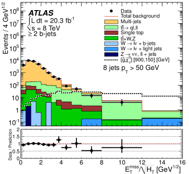
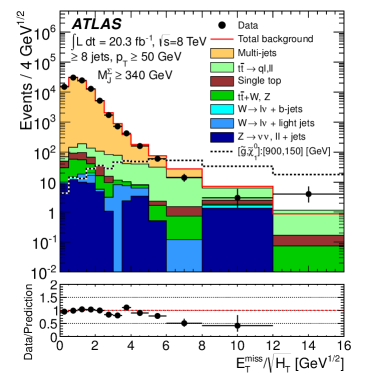
Figure 74: The $\mbox{$/{\!\!\!\!E_{\rm T}}$}/\sqrt{H_{\rm T}}$ distribution in signal regions with (a) exactly eight anti-$k_{\rm T}$ $R=0.4$ jets with $p_{\rm T}>50{\mathrm{\ Ge\kern-1.00006ptV}}$ and at least two $b$-tags and (b) at least eight anti-$k_{\rm T}$ $R=0.4$ jets with $p_{\rm T}>50{\mathrm{\ Ge\kern-1.00006ptV}}$ and the sum of the masses of anti-$k_{\rm T}$ $R=1.0$ jets in the event exceeding $340{\mathrm{\ Ge\kern-1.00006ptV}}$. The multijet prediction is taken from the measured distribution with exactly six jets and after subtracting the simulated leptonic backgrounds. The $t\bar{t}$ and $W\!$+jets backgrounds are generated with SHERPA and normalised in control regions. Single-top production is generated with MC@NLO in the $s$-channel and with AcerMC in the $t$-channel. Also shown is the distribution of a SUSY model with $m(\tilde{g})=900{\mathrm{\ Ge\kern-1.00006ptV}}$ and $m(\tilde{\chi}^{0}_{1})=150{\mathrm{\ Ge\kern-1.00006ptV}}$, generated with MadGraph+HERWIG++. From [143].

The data are interpreted in terms of different SUSY models by fitting the SM and SUSY predictions to the measured distributions in the signal and control regions. Upper limits, corresponding to $95\%$ confidence level, are set on the masses of new particles. One limit is determined for every analysis stream by taking the observed limit in the signal region with the best expected limit. The limits for the simplified SUSY model are shown separately for the $b$-tag stream and the fat jet stream in Figure 75. Gluino masses below $1210{\mathrm{\ Ge\kern-1.00006ptV}}$ and LSP masses below $480{\mathrm{\ Ge\kern-1.00006ptV}}$ are excluded. The observed limits on the gluino mass are similar for the two methods. The expected limit is better for the $b$-tag stream: by $\approx\!40{\mathrm{\ Ge\kern-1.00006ptV}}$ for the gluino mass and by $\approx\!80{\mathrm{\ Ge\kern-1.00006ptV}}$ for the LSP mass. The limit difference is covered by the uncertainty bands but since the uncertainties are strongly correlated between the two methods, the difference is significant.

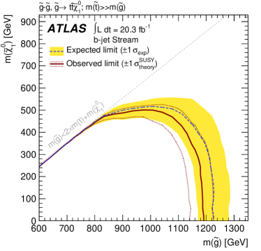
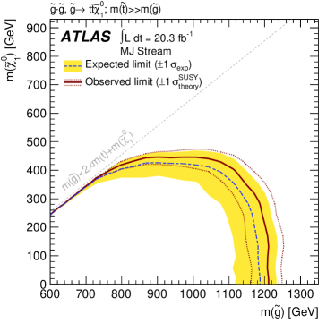
Figure 75: The $95\%$ confidence level exclusion curve (small masses are excluded) for the simplified SUSY model $\tilde{g}\rightarrow t\,\bar{t}\,\tilde{\chi}^{0}_{1}$ in the gluino-LSP mass plane for (a) the analysis stream that uses $b$-tags and (b) the stream that uses the sum of fat jet masses. For each stream, the limit from the signal region with the best expected limit is used. The theory error band contains variations of the scales and PDFs in the SUSY prediction. The experimental band contains all other uncertainties. From [143].

Why does the fat jet mass method not improve the significance as suggested by the study in Section 9.3? The most important reasons, the high jet multiplicity, the boost of the top quarks, and the size of the fat jets, are discussed in the following.

The study showed that the performance of substructure methods degrades at high jet multiplicity because a large number of jets can mimic the top quark decay signature. For prong-based taggers, larger jet combinatorics increase the chance to hit the top quark and $W$ boson mass windows. For the mass cut used in the SUSY analysis, high jet multiplicity creates a large fat jet mass because the fat jet then consists of more small-$R$ jets, all of which themselves have a mass. The shift in the fat jet mass for background events when moving from low to high $N_{\rm jet}$ is shown in Figure 53b. When substructure methods are used, the optimal sensitivity to New Physics may therefore be reached at a lower jet multiplicity than in conventional analyses.

Substructure methods work better at high boost because then more or all of the decay products are contained in the fat jet. The study in Section 9.3 was carried out for $\sqrt{s}=14{\mathrm{\ Te\kern-1.00006ptV}}$ while the analysis uses the available $\sqrt{s}=8{\mathrm{\ Te\kern-1.00006ptV}}$ data. The higher collision energy implies an increased production cross section for SUSY particles and also a larger $p_{\rm T}$ for these particles. The last point implies larger top quark $p_{\rm T}$. In addition, the gluino mass used in the study is $\approx\!100{\mathrm{\ Ge\kern-1.00006ptV}}$ larger than the exclusion limit, again increasing the boost. Lastly, the study used $\mathrm{C/A}$ fat jets with $R=1.5$. These fat jets collect more of the decay products than the anti-$k_{\rm T}$ $R=1.0$ jets used in the analysis and thereby allow for a better separation of signal from background. The $p_{\rm T}$ spectrum of the top quarks used in the study (Figure 49b) and the distance between the top quark decay quarks as shown in Figure 4 as a function of $p_{\rm T}$ together make it clear that only a small fraction of the top decays are fully captured by the $R=1.0$ jets.

In summary, substructure methods have been applied in a SUSY search and the obtained limits are close to the ones obtained by conventional methods. The greatest benefit of top tagging is achieved at low jet multiplicities and better results may be achieved by re-optimising the analysis cuts. When the LHC centre-of-mass energy is increased to $13$ and then to $14{\mathrm{\ Te\kern-1.00006ptV}}$, the boost of the hypothetical particles and the top quarks to which they decay will be larger, thereby improving the power of fat jet techniques.

11 Tagging Highly Boosted Top Quarks

Parts of this section are taken from [126], having been written by the author. The separate identification of the decay products of highly boosted top quarks becomes experimentally challenging when the detector granularity does not allow to resolve the individual particle jets. This is particularly an issue if jets are reconstructed using calorimeter information alone as it is currently done with ATLAS data. If two top quark decay jets are so close that they do not leave separate clusters then top taggers based on identifying the 3-prong decay structure will fail. This problem was addressed in [126] where a new method was proposed, the HPTTopTagger, which combines tracking and calorimeter information.

As discussed in Section 4.2, the minimal distance between two clusters in a hadronic calorimeter with $0.1\times 0.1$ cells in ($\eta,\phi)$ is $\Delta R_{\eta}=0.2$. Figure 76 shows the angular separation $\Delta R_{\eta}$ of the two closest final state quarks in hadronic top quark decay $t\rightarrow bqq$ as a function of the top quark $p_{\rm T}$. For $p_{\rm T}=1.12{\mathrm{\ Te\kern-1.00006ptV}}$ the separation is $0.2$ and calorimeter resolution issues should become apparent around that $p_{\rm T}$ or even earlier if the particle level jets that correspond to the quarks are not collimated enough to hit only a single cell.

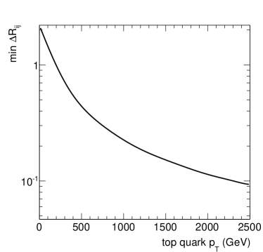
Figure 76: Angular separation $\Delta R_{\eta}=\sqrt{(\Delta\eta)^{2}+(\Delta\phi)^{2}}$ of the two closest quarks in the top quark decay $t\rightarrow bqq^{\prime}$ as a function of the top quark $p_{\rm T}$ in SM $t\bar{t}$ production generated with PYTHIA 8. From [126].

The angular resolution of a tracking detector is much better (cf. Section 4.2). The challenge for a prong-based tagger that is based on tracks is that the number of charged particles fluctuates from jet to jet. Formulating kinematic constraints to reject background is therefore difficult. The solution proposed in [126] is to use the energy $E_{\rm jet}$ measured for the fat jet in the calorimeter and compare it with the energy $E_{\rm tracks}$ of the tracks associated with the fat jet. Charged and neutral particles are included in $E_{\rm jet}$. The ratio $\alpha_{j}=E_{\rm jet}/E_{\rm tracks}$ can be used to correct for fluctuations in the charged particle fraction in the jet.

The input to the HPTTopTagger algorithm is a $\mathrm{C/A}$ $R=0.8$ calorimeter jet. The algorithm then uses the tracks with $p_{\rm T}>500{\mathrm{\ Me\kern-1.00006ptV}}$ that are associated with the jet and combines them to a track jet. The structure of the track jet is examined in a way similar to the HEPTopTagger. The track jet is decomposed into hard substructure objects using an iterative mass drop procedure with $\mu=0.8$ which ends when all substructure objects have a mass of $20{\mathrm{\ Ge\kern-1.00006ptV}}$ or less. A notable difference to the HEPTopTagger is that the HPTTopTagger does not try out all triplets of substructure objects. Instead, all track jet constituents that are part of the substructure objects are included in the filtering at once. The filter radius is given by $R_{\mathrm{filt}}=\max(0.05,\min(\Delta R_{ij}/2))$ in which $\min(\Delta R_{ij})$ is the smallest pair-wise distance of all substructure objects. The constituents of the four hardest filter jets are clustered into three subjets. The subjet momenta are scaled by $\alpha_{j}$ before kinematic cuts are applied.

ATLAS subjet calibrations and subjet simulation uncertainties exist for radius parameters $R$ between $0.2$ and $1.2$ [106]. Jets with a smaller radius parameter approach the minimal hadronic cluster size. At high top quark $p_{\rm T}$, the subjets are more collimated and their size is smaller than $R=0.2$. This problem is illustrated in [126] by modifying the HEPTopTagger to explicitly require all subjets to have $R\geq 0.2$ and setting the minimal filter radius and the minimal distance in the mass drop procedure to $0.2$. This modified algorithm is labelled HEPTopTagger^′.

The top quark tagging efficiencies of the HPTTopTagger, the HEPTopTagger, and the HEPTopTagger^′ are shown in Figure 77a as a function of the top quark $p_{\rm T}$. A top quark is taken to be tagged if a reconstructed top quark candidate is found within $\Delta R_{\eta}=0.6$ of the top quark. The generated events are passed through the Delphes simulation of the ATLAS detector. The efficiency of the HEPTopTagger^′ for finding top quarks using calorimeter cells is less than $4\%$ for $p_{\rm T}>800{\mathrm{\ Ge\kern-1.00006ptV}}$. This implies that with the present available ATLAS jet calibrations and uncertainties it is not possible to find top quarks at high $p_{\rm T}$. To obtain calibrations and uncertainties also for jets with $R<0.2$ we suggested to use the reconstructed top mass peak in $t\bar{t}$ events. The position of the peak can be used for calibration and the difference between simulation and data can serve to estimate the simulation uncertainty. At higher top quark $p_{\rm T}$ the fraction of subjets with small $R$ will be higher. This effect can be studied by binning the mass distribution in the top quark candidate $p_{\rm T}$.

The HPTTopTagger efficiency is stable at $\approx 24\%$ up to $3{\mathrm{\ Te\kern-1.00006ptV}}$ in $p_{\rm T}$. For the HEPTopTagger, the efficiency drops from $\approx 32\%$ for $800<p_{\rm T}<1000{\mathrm{\ Ge\kern-1.00006ptV}}$ to $\approx 13\%$ for $2600<p_{\rm T}<3000{\mathrm{\ Ge\kern-1.00006ptV}}$ due to the segmentation of the calorimeter which prevents all three top quark decay particle jets from being reconstructed. This is evident from Figure 77b where the top quark finding efficiency is shown for the HEPTopTagger at the particle level. When the constituents of the fat jets are stable particles, the HEPTopTagger efficiency is stable at $53\%$. If the particles are granularised into $(\eta,\phi)$ cells of size $0.1\times 0.1$, the efficiency starts to drop at a top quark $p_{\rm T}$ of $1.2{\mathrm{\ Te\kern-1.00006ptV}}$.

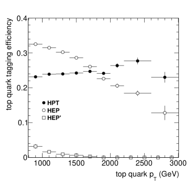
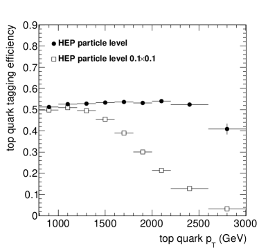
Figure 77: Efficiencies for tagging top quarks using a) calorimeter cells and b) stable particles in SM $t\bar{t}$ events generated with PYTHIA 8. For a), the events have been passed through the Delphes simulation of the ATLAS detector. Shown are results from the HPTTopTagger (HPT), the HEPTopTagger (HEP) and from a modified HEPTopTagger (HEP^′) that requires subjets to have $R\geq 0.2$. For the open markers in b), the particles are granularised into $0.1\times 0.1$ cells in $(\eta,\phi)$. From [126].

The minimal radius parameter for the filter track jets in the HPTTopTagger is taken to be 0.05. It remains to be shown what the simulation uncertainties are for such jets in the ATLAS or CMS detector. Smaller radius parameters than for calorimeter jets are possible for track jets because of the better tracking resolution. Calibrations for these jets may be obtained from hadronic decays of boosted $W$ bosons or boosted top quarks.

Ultimately, at very high top quark $p_{\rm T}$, the track reconstruction will struggle to resolve the tracks left by nearby particles. The limit is reached when hits are so close that they become part of the same reconstructed track. The track reconstruction efficiency suffers as a consequence. The ATLAS tracking efficiency is $80\%$ for $p_{\rm T}=500{\mathrm{\ Me\kern-1.00006ptV}}$ and rises to $\approx\!86\%$ for $p_{\rm T}=10{\mathrm{\ Ge\kern-1.00006ptV}}$ and higher [144, 65]. The results in [126] are obtained with a reduced tracking efficiency of $78\%$ to take the close-by effect into account. The impact of the tracking efficiency on the HPTTopTagger performance is small, however, because of the scaling to the calorimeter energy ($\alpha_{j}$).

The tagging rate is shown as a function of fat jet $p_{\rm T}$ in Figure 78a for $t\bar{t}$ signal and multijet background. For $t\bar{t}$ events, the values are similar to the top quark tagging efficiencies. The fake rate, defined as the probability to tag fat jets originating from light quarks or gluons, is stable at $1.6\%$ for the HPTTopTagger while it increases for the HEPTopTagger from $\approx 2\%$ for $p_{\rm T}=800{\mathrm{\ Ge\kern-1.00006ptV}}$ to $4.5\%$ for $p_{\rm T}=2{\mathrm{\ Te\kern-1.00006ptV}}$. The HPTTopTagger fake rate (and also the efficiency) is reduced with respect to the HEPTopTagger because not all possible triplets of substructure objects are tried. The signal-to-background ratio obtained with the HPTTopTagger is better at high $p_{\rm T}$ than that of the HEPTopTagger.

An example of an application of the HPTTopTagger in a search for New Physics is shown in Figure 78b. The signal is a leptophobic topcolor $Z^{\prime}$ boson that decays to two top quarks [33]. The width of the resonance is set to $\Gamma_{Z^{\prime}}/m_{Z^{\prime}}=3.2\%$ and the mass is $3{\mathrm{\ Te\kern-1.00006ptV}}$. The production cross section in $pp$ collisions at $\sqrt{s}=14{\mathrm{\ Te\kern-1.00006ptV}}$ is $3.5$ fb. Shown are distributions of the invariant mass $m_{12}$ of the two leading $p_{\rm T}$ top quark candidates for signal and multijet background for $300\leavevmode\nobreak\ {\rm fb}^{-1}$. This is the dominant background; SM $t\bar{t}$ production is smaller by a factor of $\approx 0.1$. The only imposed requirement is that there be at least two tagged $\mathrm{C/A}$ $R=0.8$ jets in the event. The number of signal ($S$) and background events ($B$) are compared in a mass window at the expected signal position. The signal-to-background ratio is $S/B=0.45(7)$ and the significance $S/\sqrt{B}=4.1(4)$ in the window $2560<m_{12}<3040{\mathrm{\ Ge\kern-1.00006ptV}}$. The discovery of such a $Z^{\prime}$ boson with the HPTTopTagger is therefore within reach. The uncertainties are statistical and dominated by the finite number of simulated background events. For comparison, with the same generated events, the significance when using the HEPTopTagger is only $3.3(3)$ and the difference to the HPTTopTagger results directly from the different fat jet tagging efficiencies shown in Figure 78a. The sensitivity might be improved by applying $b$-quark tagging if the related systematic uncertainties are small enough at high $p_{\rm T}$.

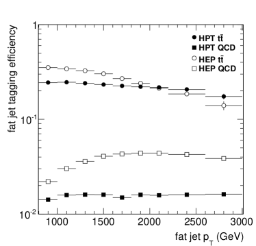
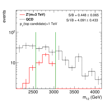
Figure 78: (a) Efficiencies for tagging $\mathrm{C/A}$ $R=0.8$ fat jets using the HPTTopTagger (HPT) and the HEPTopTagger (HEP). Shown are simulations for $t\bar{t}$ events and multijet background (QCD). (b) Invariant mass of the two leading $p_{\rm T}$ top quark candidates, reconstructed with the HPTTopTagger from 300 fb^-1 of decays of $Z^{\prime}$ bosons of mass $3{\mathrm{\ Te\kern-1.00006ptV}}$, produced in $pp$ collisions at $\sqrt{s}=14{\mathrm{\ Te\kern-1.00006ptV}}$. Also shown is the background from QCD dijet production. The signal to noise ratio $S/B$ and the significance $S/\sqrt{B}$ are given for the indicated mass window. All events are generated with PYTHIA 8 and have been passed through the Delphes simulation of the ATLAS detector. From [126].

The HPTTopTagger is a new algorithm to find boosted top quarks with transverse momentum $p_{\rm T}>1{\mathrm{\ Te\kern-1.00006ptV}}$. It combines track and calorimeter information and can find top quarks via their 3-prong decay because the finer spatial resolution of tracking detectors allows the separation of close-by particle jets that merge in the calorimeter. This tool will prove useful in analyses looking for massive particles that decay to top quarks.

12 Conclusions and Outlook

Jet structure methods that are used to identify boosted top quarks in LHC data and analyses which employ these techniques have been reviewed. The techniques are based on large (fat) jets which are used to capture all products of hadronic top quark decay $t\to bqq$.

Different classes of top quark finders are used. Energy flow taggers are based on differences in the energy sharing between particles for signal and background. The structure of background fat jets is predominantly given by soft QCD parton splitting in which the original parton retains most of the energy. The energy is more equally shared between the decay products in heavy particle decay. Substructure variables such as $k_{\rm T}$ splitting scales and jet mass are sensitive to this difference and cuts on these variables can be used to reject background. The top quark finding efficiency and the background rejection can be adjusted continuously by changing the cut value. These taggers are used in analyses with a relatively low background level. There the ability to tag top quarks with high efficiency is essential.

The second class of finders makes explicit use of the 3-prong signature of hadronic top quark decay, which often manifests itself as three distinct subjets within the large jet. Three subjets are reconstructed and then used to test kinematic relations such as the $W$ boson mass constraint. The efficiency of the prong-based tagger is lower than what is possible with energy flow taggers. This is because (a) three subjets need to be identified, and (b) the subjets have to pass the kinematic cuts. The advantage of the prong-based taggers is the small fake rate: background fat jets rarely have three hard subjets or the subjets fail the kinematic cuts. A prominent example is the HEPTopTagger with an efficiency of $40\%$ and a fake rate of $2.5\%$ for fat jets with $p_{\rm T}>400{\mathrm{\ Ge\kern-1.00006ptV}}$.

The fat jets are susceptible to contributions from underlying event and pile-up. These contributions scale with the area of the jet which is approximately proportional to $R^{2}$. The jet grooming methods that have been devised to overcome this problem have proven to be remarkably effective, as demonstrated, for example, by the pile-up stability of the reconstructed top quark mass.

The structure of background (non-top) fat jets is described within $10$–$20\%$ by Monte Carlo simulations. Substructure variables such as the jet mass are sensitive to variations of the parameters in the models for hadronisation and underlying event generation. The good description is possible only with parameters tuned to minimum bias LHC data. The best description is obtained when using HERWIG++. Significant discrepancies between simulation and data are observed in tails of distributions such as $k_{\rm T}$ splitting scales and $N$-subjettiness for PYTHIA and POWHEG+PYTHIA. These discrepancies are improved by jet grooming, indicating that the problem lies in the simulation of soft energy deposits. Whether the difference between HERWIG++ and PYTHIA is due to the hadronisation model, the underlying event model, the parton shower, or a combination of all three is unclear and more studies are needed. For example, determining to what extend the jet substructure measurements can be used to improve the tuning of the models seems to be a topic worth pursuing.

The structure of fat jets from top quark decay is well described by simulation. Differences to the data are at the level of $5\%$ for the fat jet mass. Even distribution of variables that involve many analysis steps, like the subjet invariant mass ratios of the HEPTopTagger, are well predicted. This makes it possible to apply the substructure techniques in searches for New Physics.

Limits on a technicolor $Z^{\prime}$ boson and a Kaluza-Klein gluon have been extended beyond the Tevatron limits using substructure techniques. Substructure techniques have a better $t\bar{t}$ mass resolution than conventional (resolved) top quark reconstruction methods at high $t\bar{t}$ masses where the top quark decay products are contained in the fat jet. A resolved analysis combines all small-$R$ jets without exploiting the boosted topology and often picks up a wrong small-$R$ jet as a top quark decay jet. This then spoils the reconstructed top quark mass. By considering only the subjets inside a fat jet, the combinatorics is much reduced, and the mass is reconstructed more precisely.

The search for new particles was the original impetus in [3] and [55] and substructure methods have so far been used in such searches in events with top quarks at high or intermediate $p_{\rm T}$. These searches will continue with higher statistics and at larger centre-of-mass energies. The LHC Run 2 is scheduled to start in spring 2015 with $\sqrt{s}=13{\mathrm{\ Te\kern-1.00006ptV}}$. At this high energy, the production cross section for massive particles rises and the particles will be more boosted. The angular resolution of the ATLAS and CMS calorimeters can become a limiting factor as described in Section 11 and more emphasis will likely have to be placed on the use of tracking information.

The second major driving force behind substructure techniques is the recovery of hadronic decay channels of the Higgs boson. Without substructure methods, these channels seem unpromising given the large multijet background. In the seminal paper [4], the expected significance for a Higgs boson signal at $m_{H}=125{\mathrm{\ Ge\kern-1.00006ptV}}$ is $\approx\!5\sigma$ at $\sqrt{s}=14{\mathrm{\ Te\kern-1.00006ptV}}$ and $L=30\leavevmode\nobreak\ {\rm fb}^{-1}$. The analysis used $\mathrm{C/A}$ $R=1.2$ fat jets with $p_{\rm T}>200{\mathrm{\ Ge\kern-1.00006ptV}}$ to find boosted $H\to b\bar{b}$ decays in events with $VH$ production ($V=W,Z$). In approximately $5\%$ of the $VH$ events, the Higgs boson has $p_{\rm T}>200{\mathrm{\ Ge\kern-1.00006ptV}}$. In analyses of the LHC Run 1 data ($5\leavevmode\nobreak\ {\rm fb}^{-1}$ at $\sqrt{s}=7{\mathrm{\ Te\kern-1.00006ptV}}$ and $20\leavevmode\nobreak\ {\rm fb}^{-1}$ at $8{\mathrm{\ Te\kern-1.00006ptV}}$), substructure methods do not increase the sensitivity to the Higgs boson. This is due to reduced statistics at the smaller collision energy. However, for LHC Run 2 there exists a very distinct probability to see the Higgs boson in the $b\bar{b}$ channel.

Events with $t\bar{t}H$ production can be used to determine the $t\bar{t}H$ Yukawa coupling. This process has been studied in [5] for $H\to b\bar{b}$ with one leptonic and one hadronic top quark decay. With $100\leavevmode\nobreak\ {\rm fb}^{-1}$ of data at $14{\mathrm{\ Te\kern-1.00006ptV}}$, a significance of $\approx\!4\sigma$ was found for a Higgs of mass $120{\mathrm{\ Ge\kern-1.00006ptV}}$. Also this analysis becomes feasible in Run 2.

Only substructure methods that have so far been used in physics analyses (as opposed to studies) were shown in this review. There are many more recently proposed methods. Examples are shower deconstruction [145, 146] and Q-jets [147], which statistically analyse the clustering history in jets. Q-jets have been studied with ATLAS [148] and for an efficiency to tag boosted hadronically decaying $W$ bosons of $50\%$, the rejection of multijet background is 15.

The field of jet substructure is new and it evolves through a close collaboration of theoretical and experimental particle physicists. In the short time of its existence it has become a proven integral part of the analysis tool set at the LHC. Jet structure techniques will become more important in the next years with the LHC running at full design energy and they will enhance the physics potential and reach at the energy frontier.

Danksagung

Viele der Ergebnisse, die in dieser Habilitationsschrift dokumentiert sind, wurden während der zurückliegenden vier Jahre in der ATLAS-Arbeitsgruppe von Prof. Dr. André Schöning am Physikalischen Institut der Universität Heidelberg erarbeitet.

Ich danke Prof. Schöning für die Weitsicht, mit der er frühzeitig das Potential des Felds Jetstruktur erkannt hat, und für das Herstellen des Kontakts zu Prof. Plehn vom Theoretischen Institut. Ich danke ihm auch für das mir entgegengebrachte Vertrauen, die Forschung eigenständig zu betreiben, für Anregungen und Diskussionen sowie für seine uneingeschränkte Unterstützung bei der systematischen Ausweitung des Arbeitsgebiets und dem Aufbau der Arbeitsgruppe.

Ich danke den Mitgliedern der HEPTopTagger-Arbeitsgruppe am Physikalischen Institut, Dr. Gregor Kasieczka, Dr. Christoph Anders, Maddalena Giulini und David Sosa, für die sehr fruchtbare Zusammenarbeit und den hohen Einsatz, mit dem sie publikationsreife Ergebnisse erarbeiten.

Ich danke den Theoretischen Physikern Prof. Dr. Tilman Plehn, Dr. Michael Spannowsky, Dr. Michihisa Takeuchi und Torben Schell für die exzellente Zusammenarbeit. Insbesondere die Diskussionen mit Prof. Plehn und Dr. Spannowsky haben entscheidend zur Qualität der Analysen beigetragen.

Ich danke auch den Mitgliedern der Arbeitsgruppe Jet Substructure der ATLAS-Kollaboration, insbesondere Dr. David Miller, Dr. Adam Davison und Dr. Emily Thompson für Diskussionen, Hilfe und Unterstützung.

Nicht zuletzt danke ich meiner Familie für ihren Rückhalt und ihre Unterstützung.

References

- [1] ATLAS Collaboration, Observation of a new particle in the search for the Standard Model Higgs boson with the ATLAS detector at the LHC, Phys. Lett. B716 (2012) 1–29, arXiv:1207.7214 [hep-ex].
- [2] CMS Collaboration, Observation of a new boson at a mass of 125 GeV with the CMS experiment at the LHC, Phys. Lett. B716 (2012) 30–61, arXiv:1207.7235 [hep-ex].
- [3] M. H. Seymour, Searches for new particles using cone and cluster jet algorithms: A Comparative study, Z. Phys. C62 (1994) 127–138.
- [4] J. M. Butterworth, A. R. Davison, M. Rubin, and G. P. Salam, Jet substructure as a new Higgs search channel at the LHC, Phys. Rev. Lett. 100 (2008) 242001, arXiv:0802.2470 [hep-ph].
- [5] T. Plehn, G. P. Salam, and M. Spannowsky, Fat Jets for a Light Higgs, Phys. Rev. Lett. 104 (2010) 111801, arXiv:0910.5472 [hep-ph].
- [6] A. Abdesselam, E. B. Kuutmann, U. Bitenc, G. Brooijmans, J. Butterworth, et al., Boosted objects: A Probe of beyond the Standard Model physics, Eur. Phys. J. C71 (2011) 1661, arXiv:1012.5412 [hep-ph].
- [7] A. Altheimer, S. Arora, L. Asquith, G. Brooijmans, J. Butterworth, et al., Jet Substructure at the Tevatron and LHC: New results, new tools, new benchmarks, J. Phys. G39 (2012) 063001, arXiv:1201.0008 [hep-ph].
- [8] T. Plehn and M. Spannowsky, Top Tagging, J. Phys. G39 (2012) 083001, arXiv:1112.4441 [hep-ph].
- [9] F.-P. Schilling, Top Quark Physics at the LHC: A Review of the First Two Years, Int. J. Mod. Phys. A27 (2012) 1230016, arXiv:1206.4484 [hep-ex].
- [10] Particle Data Group, Review of Particle Physics, Phys. Rev. D86 (2012) 010001.
- [11] Particle Data Group, 2013 partial update for the 2014 edition, http://pdg.lbl.gov.
- [12] ATLAS Collaboration, Measurement of the Inelastic Proton-Proton Cross-Section at TeV with the ATLAS Detector, Nature Commun. 2 (2011) 463, arXiv:1104.0326 [hep-ex].
- [13] A. Martin, W. Stirling, R. Thorne, and G. Watt, Parton distributions for the LHC, Eur. Phys. J. C63 (2009) 189–285, arXiv:0901.0002 [hep-ph].
- [14] M. Aliev, H. Lacker, U. Langenfeld, S. Moch, P. Uwer, et al., HATHOR: HAdronic Top and Heavy quarks crOss section calculatoR, Comput. Phys. Commun. 182 (2011) 1034–1046, arXiv:1007.1327 [hep-ph].
- [15] J. M. Campbell, J. Huston, and W. Stirling, Hard Interactions of Quarks and Gluons: A Primer for LHC Physics, Rept. Prog. Phys. 70 (2007) 89, arXiv:hep-ph/0611148 [hep-ph].
- [16] ATLAS Collaboration, Physics Summary Plots, 2013. https://twiki.cern.ch/twiki/bin/view/AtlasPublic/CombinedSummaryPlots.
- [17] T. M. Liss and A. Quadt, The Top Quark, in [10], p. 596.
- [18] G. P. Salam, Theory of Fat Jets and Jet Substructure, Invited talk at Higgs Hunting 2012, July, 2012. http://www.higgshunting.fr/.
- [19] T. Plehn, M. Spannowsky, M. Takeuchi, and D. Zerwas, Stop Reconstruction with Tagged Tops, JHEP 1010 (2010) 078, arXiv:1006.2833 [hep-ph].
- [20] C. T. Hill and E. H. Simmons, Strong dynamics and electroweak symmetry breaking, Phys. Rept. 381 (2003) 235–402, arXiv:hep-ph/0203079 [hep-ph].
- [21] P. Fayet, Supersymmetry and Weak, Electromagnetic and Strong Interactions, Phys. Lett. B64 (1976) 159.
- [22] P. Fayet, Spontaneously Broken Supersymmetric Theories of Weak, Electromagnetic and Strong Interactions, Phys. Lett. B69 (1977) 489.
- [23] G. R. Farrar and P. Fayet, Phenomenology of the Production, Decay, and Detection of New Hadronic States Associated with Supersymmetry, Phys. Lett. B76 (1978) 575–579.
- [24] P. Fayet, Relations Between the Masses of the Superpartners of Leptons and Quarks, the Goldstino Couplings and the Neutral Currents, Phys. Lett. B84 (1979) 416.
- [25] S. Dimopoulos and H. Georgi, Softly Broken Supersymmetry and SU(5), Nucl. Phys. B193 (1981) 150.
- [26] M. Schmaltz and D. Tucker-Smith, Little Higgs review, Ann. Rev. Nucl. Part. Sci. 55 (2005) 229–270, arXiv:hep-ph/0502182 [hep-ph].
- [27] N. Arkani-Hamed, A. G. Cohen, and H. Georgi, Electroweak symmetry breaking from dimensional deconstruction, Phys. Lett. B513 (2001) 232–240, arXiv:hep-ph/0105239 [hep-ph].
- [28] S. Weinberg, Implications of Dynamical Symmetry Breaking, Phys. Rev. D13 (1976) 974–996.
- [29] L. Susskind, Dynamics of Spontaneous Symmetry Breaking in the Weinberg-Salam Theory, Phys. Rev. D20 (1979) 2619–2625.
- [30] F. Mandl and G. Shaw, Quantum Field Theory. 1984.
- [31] C. T. Hill, Topcolor: Top quark condensation in a gauge extension of the standard model, Phys. Lett. B266 (1991) 419–424.
- [32] C. T. Hill, Topcolor assisted technicolor, Phys. Lett. B345 (1995) 483–489, arXiv:hep-ph/9411426 [hep-ph].
- [33] R. M. Harris, C. T. Hill, and S. J. Parke, Cross-section for topcolor decaying to , arXiv:hep-ph/9911288 [hep-ph].
- [34] L. Randall and R. Sundrum, A Large mass hierarchy from a small extra dimension, Phys. Rev. Lett. 83 (1999) 3370–3373, arXiv:hep-ph/9905221 [hep-ph].
- [35] L. Randall and R. Sundrum, An Alternative to compactification, Phys. Rev. Lett. 83 (1999) 4690–4693, arXiv:hep-th/9906064 [hep-th].
- [36] D. E. Morrissey, T. Plehn, and T. M. Tait, Physics searches at the LHC, Phys. Rept. 515 (2012) 1–113, arXiv:0912.3259 [hep-ph].
- [37] G. F. Giudice and J. D. Wells, Extra Dimensions, in [10], p. 1354.
- [38] A. Sellerholm, Kaluza-Klein Theories, 2005. http://courses.theophys.kth.se/5A1381/reports/sellerholm.pdf.
- [39] T. Kaluza, Zum Unitätsproblem der Physik, Sitzungsber. Preuss. Akad. Wiss. Berlin (Math.Phys.) 1921 (1921) 966–972. https://archive.org/details/sitzungsberichte1921preussi.
- [40] O. Klein, Quantentheorie und fünfdimensionale Relativitätstheorie, Z. Phys. 37 (1926) 895–906.
- [41] B. Lillie, L. Randall, and L.-T. Wang, The Bulk RS KK-gluon at the LHC, JHEP 0709 (2007) 074, arXiv:hep-ph/0701166 [hep-ph].
- [42] G. F. Sterman and S. Weinberg, Jets from Quantum Chromodynamics, Phys. Rev. Lett. 39 (1977) 1436.
- [43] UA1 Collaboration, Hadronic Jet Production at the CERN Proton - anti-Proton Collider, Phys. Lett. B132 (1983) 214.
- [44] G. P. Salam, Towards Jetography, Eur. Phys. J. C67 (2010) 637–686, arXiv:0906.1833 [hep-ph].
- [45] Y. L. Dokshitzer, G. Leder, S. Moretti, and B. Webber, Better jet clustering algorithms, JHEP 08 (1997) 001, arXiv:hep-ph/9707323 [hep-ph].
- [46] M. Wobisch and T. Wengler, Hadronization corrections to jet cross sections in deep- inelastic scattering, arXiv:hep-ph/9907280 [hep-ph].
- [47] M. Wobisch, Measurement and QCD Analysis of Jet Cross Sections in Deep-Inelastic Positron-Proton Collisions at = 300 GeV. PhD thesis, Rheinisch-Westfälische Technische Hochschule Aachen, Germany, 2000. http://www-h1.desy.de/psfiles/theses/h1th-201.pdf.
- [48] S. Catani, Y. L. Dokshitzer, M. Olsson, G. Turnock, and B. Webber, New clustering algorithm for multi-jet cross-sections in annihilation, Phys. Lett. B 269 (1991) 432.
- [49] S. D. Ellis and D. E. Soper, Successive combination jet algorithm for hadron collisions, Phys. Rev. D 48 (1993) 3160, arXiv:hep-ph/9305266 [hep-ph].
- [50] S. Catani, Y. L. Dokshitzer, M. Seymour, and B. Webber, Longitudinally invariant clustering algorithms for hadron hadron collisions, Nucl. Phys. B 406 (1993) 187.
- [51] M. Cacciari, G. P. Salam, and G. Soyez, The anti-kt jet clustering algorithm, JHEP 04 (2008) 063, arXiv:0802.1189 [hep-ph].
- [52] G. Marchesini, B. Webber, G. Abbiendi, I. Knowles, M. Seymour, et al., HERWIG: A Monte Carlo event generator for simulating hadron emission reactions with interfering gluons. Version 5.1 - April 1991, Comput. Phys. Commun. 67 (1992) 465–508.
- [53] G. Altarelli and G. Parisi, Asymptotic Freedom in Parton Language, Nucl. Phys. B126 (1977) 298.
- [54] ATLAS Collaboration, Jet mass and substructure of inclusive jets in = 7 TeV collisions with the ATLAS experiment, JHEP 1205 (2012) 128, arXiv:1203.4606 [hep-ex].
- [55] J. Butterworth, B. Cox, and J. R. Forshaw, scattering at the CERN LHC, Phys. Rev. D65 (2002) 096014, arXiv:hep-ph/0201098 [hep-ph].
- [56] S. Ellis, J. Huston, K. Hatakeyama, P. Loch, and M. Tonnesmann, Jets in hadron-hadron collisions, Prog. Part. Nucl. Phys. 60 (2008) 484–551, arXiv:0712.2447 [hep-ph].
- [57] M. Dasgupta, L. Magnea, and G. P. Salam, Non-perturbative QCD effects in jets at hadron colliders, JHEP 0802 (2008) 055, arXiv:0712.3014 [hep-ph].
- [58] D. Krohn, J. Thaler, and L.-T. Wang, Jet Trimming, JHEP 1002 (2010) 084, arXiv:0912.1342 [hep-ph].
- [59] S. D. Ellis, C. K. Vermilion, and J. R. Walsh, Techniques for improved heavy particle searches with jet substructure, Phys. Rev. D80 (2009) 051501, arXiv:0903.5081 [hep-ph].
- [60] S. D. Ellis, C. K. Vermilion, and J. R. Walsh, Recombination Algorithms and Jet Substructure: Pruning as a Tool for Heavy Particle Searches, Phys. Rev. D81 (2010) 094023, arXiv:0912.0033 [hep-ph].
- [61] L. Ponce, LHC Accelerator Performance and Plans, 165th CERN Council Meeting, Dec 2012. https://indico.cern.ch/conferenceDisplay.py?confId=218449.
- [62] ATLAS Collaboration, Public Luminosity Results, 2013. https://twiki.cern.ch/twiki/bin/view/AtlasPublic/LuminosityPublicResults.
- [63] ATLAS Collaboration, The ATLAS Experiment at the CERN Large Hadron Collider, JINST 3 (2008) S08003.
- [64] ATLAS Collaboration, Performance of the ATLAS Detector using First Collision Data, JHEP 1009 (2010) 056, arXiv:1005.5254 [hep-ex].
- [65] ATLAS Collaboration, Charged-particle multiplicities in pp interactions measured with the ATLAS detector at the LHC, New J. Phys. 13 (2011) 053033, arXiv:1012.5104 [hep-ex].
- [66] ATLAS Collaboration, Single hadron response measurement and calorimeter jet energy scale uncertainty with the ATLAS detector at the LHC, Eur. Phys. J. C73 (2013) 2305, arXiv:1203.1302 [hep-ex].
- [67] CMS Collaboration, The CMS experiment at the CERN LHC, JINST 3 (2008) S08004.
- [68] CMS Collaboration, Particle-Flow Event Reconstruction in CMS and Performance for Jets, Taus, and MET, CMS-PAS-PFT-09-001. https://cds.cern.ch/record/1194487.
- [69] CMS Collaboration, Commissioning of the Particle-Flow reconstruction in Minimum-Bias and Jet Events from pp Collisions at 7 TeV, CMS-PAS-PFT-10-002. https://cds.cern.ch/record/1279341.
- [70] T. Sjostrand, S. Mrenna, and P. Z. Skands, PYTHIA 6.4 Physics and Manual, JHEP 0605 (2006) 026, arXiv:hep-ph/0603175 [hep-ph].
- [71] T. Sjostrand, S. Mrenna, and P. Z. Skands, A Brief Introduction to PYTHIA 8.1, Comput. Phys. Commun. 178 (2008) 852–867, arXiv:0710.3820 [hep-ph].
- [72] R. Corke and T. Sjostrand, Improved Parton Showers at Large Transverse Momenta, Eur. Phys. J. C 69 (2010) 1–18, arXiv:1003.2384 [hep-ph].
- [73] T. Sjostrand, Monte Carlo Generators, arXiv:hep-ph/0611247 [hep-ph].
- [74] B. Andersson, G. Gustafson, G. Ingelman, and T. Sjostrand, Parton Fragmentation and String Dynamics, Phys. Rept. 97 (1983) 31–145.
- [75] ATLAS Collaboration, ATLAS tunes of PYTHIA 6 and PYTHIA 8 for MC11, ATL-PHYS-PUB-2011-009. https://cds.cern.ch/record/1363300.
- [76] ATLAS Collaboration, New ATLAS event generator tunes to 2010 data, ATL-PHYS-PUB-2011-008. https://cdsweb.cern.ch/record/1345343.
- [77] G. Marchesini and B. Webber, Monte Carlo Simulation of General Hard Processes with Coherent QCD Radiation, Nucl. Phys. B310 (1988) 461.
- [78] G. Corcella, I. Knowles, G. Marchesini, S. Moretti, K. Odagiri, et al., HERWIG 6.5 release note, arXiv:hep-ph/0210213 [hep-ph].
- [79] B. Webber, A QCD Model for Jet Fragmentation Including Soft Gluon Interference, Nucl. Phys. B238 (1984) 492.
- [80] J. M. Butterworth, J. R. Forshaw, and M. H. Seymour, Multiparton interactions in photoproduction at HERA, Z. Phys. C 72 (1996) 637, arXiv:9601371 [hep-ph].
- [81] ATLAS Collaboration, First tuning of HERWIG/JIMMY to ATLAS data, ATL-PHYS-PUB-2010-014. http://cdsweb.cern.ch/record/1303025.
- [82] M. Bahr et al., Herwig++ physics and manual, Eur. Phys. J. C 58 (2008) 639, arXiv:0803.0883 [hep-ph].
- [83] M. Bahr, S. Gieseke, and M. H. Seymour, Simulation of multiple partonic interactions in Herwig++, JHEP 0807 (2008) 076, arXiv:0803.3633 [hep-ph].
- [84] S. Frixione and B. R. Webber, Matching NLO QCD computations and parton shower simulations, JHEP 06 (2002) 029, arXiv:hep-ph/0204244 [hep-ph].
- [85] S. Frixione, P. Nason, and C. Oleari, Matching NLO QCD computations with Parton Shower simulations: the POWHEG method, JHEP 11 (2007) 070, arXiv:0709.2092 [hep-ph].
- [86] F. Krauss, R. Kuhn, and G. Soff, AMEGIC++ 1.0: A Matrix element generator in C++, JHEP 0202 (2002) 044, arXiv:hep-ph/0109036 [hep-ph].
- [87] T. Gleisberg, S. Hoeche, F. Krauss, A. Schalicke, S. Schumann, et al., SHERPA 1. alpha: A Proof of concept version, JHEP 0402 (2004) 056, arXiv:hep-ph/0311263 [hep-ph].
- [88] T. Gleisberg, S. Hoeche, F. Krauss, M. Schonherr, S. Schumann, et al., Event generation with SHERPA 1.1, JHEP 0902 (2009) 007, arXiv:0811.4622 [hep-ph].
- [89] M. L. Mangano, M. Moretti, F. Piccinini, R. Pittau, and A. D. Polosa, ALPGEN, a generator for hard multiparton processes in hadronic collisions, JHEP 0307 (2003) 001, arXiv:hep-ph/0206293 [hep-ph].
- [90] T. Stelzer and W. Long, Automatic generation of tree level helicity amplitudes, Comput. Phys. Commun. 81 (1994) 357–371, arXiv:hep-ph/9401258 [hep-ph].
- [91] J. Alwall, P. Demin, S. de Visscher, R. Frederix, M. Herquet, et al., MadGraph/MadEvent v4: The New Web Generation, JHEP 0709 (2007) 028, arXiv:0706.2334 [hep-ph].
- [92] B. P. Kersevan and E. Richter-Was, The Monte Carlo event generator AcerMC version 2.0 with interfaces to PYTHIA 6.2 and HERWIG 6.5, arXiv:hep-ph/0405247 [hep-ph].
- [93] GEANT4 Collaboration, GEANT4: A Simulation toolkit, Nucl. Instrum. Meth. A506 (2003) 250–303.
- [94] E. Richter-Was, AcerDET: A Particle level fast simulation and reconstruction package for phenomenological studies on high physics at LHC, arXiv:hep-ph/0207355 [hep-ph].
- [95] S. Ovyn, X. Rouby, and V. Lemaitre, DELPHES, a framework for fast simulation of a generic collider experiment, arXiv:0903.2225 [hep-ph].
- [96] J. de Favereau, C. Delaere, P. Demin, A. Giammanco, V. Lemaître, et al., DELPHES 3, A modular framework for fast simulation of a generic collider experiment, arXiv:1307.6346 [hep-ex].
- [97] J. Conway et al., PGS 4 – Pretty Good Simulation of high energy collisions, 2006. http://www.physics.ucdavis.edu/~conway/research/software/pgs/pgs4-general.htm.
- [98] M. Cacciari and G. P. Salam, Dispelling the myth for the jet-finder, Phys. Lett. B641 (2006) 57–61, arXiv:hep-ph/0512210 [hep-ph].
- [99] M. Cacciari, G. P. Salam, and G. Soyez, FastJet User Manual, Eur. Phys. J. C72 (2012) 1896, arXiv:1111.6097 [hep-ph].
- [100] ATLAS Collaboration, Jet energy measurement with the ATLAS detector in proton-proton collisions at = 7 TeV, Eur. Phys. J. C73 (2013) 2304, arXiv:1112.6426 [hep-ex].
- [101] ATLAS Collaboration, Jet energy scale and its systematic uncertainty in proton-proton collisions at = 7 TeV with ATLAS 2011 data, ATLAS-CONF-2013-004. http://cdsweb.cern.ch/record/1509552.
- [102] ATLAS Collaboration, Performance of boosted top quark identification in 2012 ATLAS data, ATLAS-CONF-2013-084. https://cds.cern.ch/record/1571040.
- [103] M. Cacciari and G. P. Salam, Pileup subtraction using jet areas, Phys. Lett. B659 (2008) 119–126, arXiv:0707.1378 [hep-ph].
- [104] ATLAS Collaboration, Pile-up subtraction and suppression for jets in ATLAS, ATLAS-CONF-2013-083. https://cds.cern.ch/record/1570994.
- [105] M. Cacciari, G. P. Salam, and G. Soyez, The Catchment Area of Jets, JHEP 04 (2008) 005, arXiv:0802.1188 [hep-ph].
- [106] ATLAS Collaboration, Performance of jet substructure techniques for large- jets in proton-proton collisions at = 7 TeV using the ATLAS detector, JHEP 1309 (2013) 076, arXiv:1306.4945 [hep-ex].
- [107] S. Schätzel, Calibration of HEPTopTagger Jets in ATLAS, ATL-COM-PHYS-2012-1461. https://cds.cern.ch/record/1483209. Accessible only for ATLAS members.
- [108] S. Schätzel, Jet Resolution for HEPTopTagger Jets in ATLAS, ATL-COM-PHYS-2012-1463. https://cds.cern.ch/record/1483229. Accessible only for ATLAS members.
- [109] ATLAS Collaboration, Measurement of the b-tag Efficiency in a Sample of Jets Containing Muons with 5 fb-1 of Data from the ATLAS Detector, ATLAS-CONF-2012-043. https://cds.cern.ch/record/1435197.
- [110] ATLAS Collaboration, Measuring the b-tag efficiency in a top-pair sample with 4.7 fb-1 of data from the ATLAS detector, ATLAS-CONF-2012-097. https://cds.cern.ch/record/1460443.
- [111] ATLAS Collaboration, Measurement of the Mistag Rate with 5 fb-1 of Data Collected by the ATLAS Detector, ATLAS-CONF-2012-040. https://cds.cern.ch/record/1435194.
- [112] CMS Collaboration, Determination of Jet Energy Calibration and Transverse Momentum Resolution in CMS, JINST 6 (2011) P11002, arXiv:1107.4277 [physics.ins-det].
- [113] D0 Collaboration, Determination of the absolute jet energy scale in the D0 calorimeters, Nucl. Instrum. Meth. A424 (1999) 352–394, arXiv:hep-ex/9805009 [hep-ex].
- [114] CMS Collaboration, The Jet Plus Tracks Algorithm for Calorimeter Jet Energy Corrections in CMS, CMS-PAS-JME-09-002. https://cds.cern.ch/record/1190234.
- [115] L. G. Almeida, S. J. Lee, G. Perez, G. Sterman, and I. Sung, Template Overlap Method for Massive Jets, Phys. Rev. D82 (2010) 054034, arXiv:1006.2035 [hep-ph].
- [116] L. G. Almeida, O. Erdogan, J. Juknevich, S. J. Lee, G. Perez, et al., Three-particle templates for a boosted Higgs boson, Phys. Rev. D85 (2012) 114046, arXiv:1112.1957 [hep-ph].
- [117] ATLAS Collaboration, Search for resonances decaying into top-quark pairs using fully hadronic decays in collisions with ATLAS at = 7 TeV, JHEP 1301 (2013) 116, arXiv:1211.2202 [hep-ex].
- [118] R. Alon, E. Duchovni, G. Perez, A. P. Pranko, and P. K. Sinervo, A Data-driven method of pile-up correction for the substructure of massive jets, Phys. Rev. D84 (2011) 114025, arXiv:1101.3002 [hep-ph].
- [119] CDF Collaboration, Study of Substructure of High Transverse Momentum Jets Produced in Proton-Antiproton Collisions at = 1.96 TeV, Phys. Rev. D85 (2012) 091101, arXiv:1106.5952 [hep-ex].
- [120] D. E. Kaplan, K. Rehermann, M. D. Schwartz, and B. Tweedie, Top Tagging: A Method for Identifying Boosted Hadronically Decaying Top Quarks, Phys. Rev. Lett. 101 (2008) 142001, arXiv:0806.0848 [hep-ph].
- [121] CMS Collaboration, A Cambridge-Aachen (C-A) based Jet Algorithm for boosted top-jet tagging, CMS-PAS-JME-09-001. https://cds.cern.ch/record/1194489.
- [122] CMS Collaboration, Search for anomalous t t-bar production in the highly-boosted all-hadronic final state, JHEP 1209 (2012) 029, arXiv:1204.2488 [hep-ex].
- [123] T. Plehn, M. Spannowsky, and M. Takeuchi, How to Improve Top Tagging, Phys. Rev. D85 (2012) 034029, arXiv:1111.5034 [hep-ph].
- [124] ATLAS Collaboration, Measurement of the W boson polarization in top quark decays with the ATLAS detector, JHEP 1206 (2012) 088, arXiv:1205.2484 [hep-ex].
- [125] S. Gieseke, C. Rohr, and A. Siodmok, Colour reconnections in Herwig++, Eur. Phys. J. C 72 (2012) 2225, arXiv:1206.0041 [hep-ph].
- [126] S. Schätzel and M. Spannowsky, Tagging highly boosted top quarks, Phys. Rev. D89 (2014) 014007, arXiv:1308.0540 [hep-ph].
- [127] ATLAS Collaboration, A search for resonances in the lepton plus jets final state with ATLAS using 4.7 fb-1 of pp collisions at = 7 TeV, Phys. Rev. D88 (2013) 012004, arXiv:1305.2756 [hep-ex].
- [128] ATLAS Collaboration, A search for resonances in lepton plus jets events with ATLAS using 14 fb-1 of proton-proton collisions at =8 TeV, ATLAS-CONF-2013-052. http://cdsweb.cern.ch/record/1547568.
- [129] A. Hook, E. Izaguirre, M. Lisanti, and J. G. Wacker, High Multiplicity Searches at the LHC Using Jet Masses, Phys. Rev. D85 (2012) 055029, arXiv:1202.0558 [hep-ph].
- [130] S. El Hedri, A. Hook, M. Jankowiak, and J. G. Wacker, Learning How to Count: A High Multiplicity Search for the LHC, JHEP 1308 (2013) 136, arXiv:1302.1870 [hep-ph].
- [131] D0 Collaboration, Search for a Narrow Resonance in Collisions at = 1.96 TeV, Phys. Rev. D85 (2012) 051101, arXiv:1111.1271 [hep-ex].
- [132] CDF Collaboration, A Search for resonant production of pairs in of integrated luminosity of collisions at = 1.96 TeV, Phys. Rev. D84 (2011) 072004, arXiv:1107.5063 [hep-ex].
- [133] CDF Collaboration, Search for resonant production of decaying to jets in collisions at = 1.96 TeV, Phys. Rev. D84 (2011) 072003, arXiv:1108.4755 [hep-ex].
- [134] CDF Collaboration, Search for Resonant Production in the Semi-leptonic Decay Mode Using the Full CDF Data Set, Phys. Rev. Lett. 110 (2013) 121802, arXiv:1211.5363 [hep-ex].
- [135] R. M. Harris and S. Jain, Cross Sections for Leptophobic Topcolor Z’ Decaying to Top-Antitop, Eur. Phys. J. C72 (2012) 2072, arXiv:1112.4928 [hep-ph].
- [136] B. Lillie, J. Shu, and T. M. Tait, Kaluza-Klein Gluons as a Diagnostic of Warped Models, Phys. Rev. D76 (2007) 115016, arXiv:0706.3960 [hep-ph].
- [137] K. Agashe, A. Belyaev, T. Krupovnickas, G. Perez, and J. Virzi, LHC Signals from Warped Extra Dimensions, Phys. Rev. D77 (2008) 015003, arXiv:hep-ph/0612015 [hep-ph].
- [138] A. Djouadi, G. Moreau, and R. K. Singh, Kaluza-Klein excitations of gauge bosons at the LHC, Nucl. Phys. B797 (2008) 1–26, arXiv:0706.4191 [hep-ph].
- [139] K. Agashe, H. Davoudiasl, G. Perez, and A. Soni, Warped Gravitons at the LHC and Beyond, Phys. Rev. D76 (2007) 036006, arXiv:hep-ph/0701186 [hep-ph].
- [140] CMS Collaboration, Search for resonant production in lepton+jets events in collisions at = 7 TeV, JHEP 1212 (2012) 015, arXiv:1209.4397 [hep-ex].
- [141] CMS Collaboration, Searches for anomalous ttbar production in pp collisions at =8 TeV, arXiv:1309.2030 [hep-ex].
- [142] G. Kasieczka, Search for Resonances Decaying into Top Quark Pairs Using Fully Hadronic Decays in pp Collisions with ATLAS at = 7 TeV. PhD thesis, Universität Heidelberg, Germany, 2013. http://www.physi.uni-heidelberg.de/Publications/Kasieczka-Doktor.pdf.
- [143] ATLAS Collaboration, Search for new phenomena in final states with large jet multiplicities and missing transverse momentum at = 8 TeV proton-proton collisions using the ATLAS experiment, arXiv:1308.1841 [hep-ex].
- [144] ATLAS Collaboration, Charged-particle multiplicities in interactions at = 900 GeV measured with the ATLAS detector at the LHC, Phys. Lett. B688 (2010) 21–42, arXiv:1003.3124 [hep-ex].
- [145] D. E. Soper and M. Spannowsky, Finding physics signals with shower deconstruction, Phys. Rev. D84 (2011) 074002, arXiv:1102.3480 [hep-ph].
- [146] D. E. Soper and M. Spannowsky, Finding top quarks with shower deconstruction, Phys. Rev. D87 (2013) 054012, arXiv:1211.3140 [hep-ph].
- [147] S. D. Ellis, A. Hornig, T. S. Roy, D. Krohn, and M. D. Schwartz, Q-jets: A Non-Deterministic Approach to Tree-Based Jet Substructure, Phys. Rev. Lett. 108 (2012) 182003, arXiv:1201.1914 [hep-ph].
- [148] ATLAS Collaboration, Performance and Validation of Q-Jets at the ATLAS Detector in pp Collisions at = 8 TeV in 2012, ATLAS-CONF-2013-087. http://cds.cern.ch/record/1572981.