Transport Signatures of Majorana Quantum Criticality Realized by Dissipative Resonant Tunneling

Abstract

We consider theoretically the transport properties of a spinless resonant electronic level coupled to strongly dissipative leads, in the regime of circuit impedance near the resistance quantum. Using the Luttinger liquid analogy, one obtains an effective Hamiltonian expressed in terms of interacting Majorana fermions, in which all environmental degrees of freedom (leads and electromagnetic modes) are encapsulated in a single fermionic bath. General transport equations for this system are then derived in terms of the Majorana T-matrix. Perturbative treatment of the Majorana interaction term yields the appearance of a marginal, linear dependence of the conductance on temperature when the system is tuned to its quantum critical point, in agreement with recent experimental observations. We investigate in detail the different crossovers involved in the problem, and analyze the role of the interaction terms in the transport scaling functions. In particular, we show that single barrier scaling applies when the system is slightly tuned away from its Majorana critical point, strengthening the general picture of dynamical Coulomb blockade.

I Introduction

Engineering electronic systems at the nanoscale is becoming a fascinating way to realize unconventional states of matter, ones that break the Fermi liquid paradigm. Some recent examples include several ways of realizing one-dimensional Luttinger liquid physics Chang (2003); Deshpande et al. (2010); Blumenstein et al. (2011); Laroche et al. (2014), gate-tunable molecules showing quantum phase transitions Roch et al. (2009); Florens et al. (2011), and tailored double quantum dots in semiconductors exhibiting complex behaviors such as multichannel Kondo physics Grobis et al. (2007); Potok et al. (2007). Further progress and new classes of anomalous behavior can be realized by combining both fine-tuned nanostructures and tailored environments, as demonstrated by a series of recent experiments Parmentier et al. (2011); Mebrahtu et al. (2012, 2013); Jezouin et al. (2013) involving quantum tunneling at the nanoscale in the presence of strong dissipation in the contacts. In this type of system, single electron tunneling events create large electromagnetic fluctuations, that become energetically prohibitive in a strongly resistive circuit. This so-called dynamical Coulomb blockade phenomenon leads to inelastic losses that can be quite effective in impeding low-energy electrons from transporting current, and so dramatically depress the conductance for small applied voltage bias across the device (typically in a power-law fashion). This physical behavior is quite reminiscent of the problem of quantum tunneling in Luttinger liquids, one-dimensional conducting wires where Coulomb interaction effects are prominent Giamarchi (2004). In that case, power-law zero-bias anomalies in transport also arise due to excitations of collective plasmon modes. This analogy can be formally pushed to a general theoretical equivalence between the two problems using bosonization techniques Safi and Saleur (2004), which makes dissipative circuits an attractive method for probing local aspects of Luttinger liquid physics in nanocircuits.

Recent experimental investigations further explored this analogy by extending previous single barrier devices to quantum dot systems Mebrahtu et al. (2012, 2013). Here, additional quantum degrees of freedom are introduced, such as the quantized charge and magnetic moment for the localized electronic level. Previous theoretical arguments Mebrahtu et al. (2012); Florens et al. (2007) showed that the Luttinger analogy is still maintained, opening an interesting playground for quantum critical and anomalous Kondo-type behavior.

In the present paper, we aim at analyzing in detail the transport characteristics in the simpler case when only the local electron charge is the relevant variable, as can be realized by a full spin-polarization of the electronic states in a large magnetic field. This situation results in complex signatures because zero bias anomalies are very sensitive to the typical transmission through the device. They can, for instance, be washed out when the transmission of the electron channel approaches unity. While the complete loss of dynamical Coulomb blockade at perfect transmission is correct for single tunnel barriers, it turns out to be quite non-trivial in the case of resonant tunneling through a perfectly transmitting electronic level.

We show here that full transmission does survive large dissipation in the contacts, but extra energy loss in the environment is still possible which then modifies the low-temperature behavior of the conductance. This behavior can be rationalized when the dissipation is fine-tuned such that the impedance is close to the quantum value $h/e^{2}$ (here $h$ is Planck’s constant and $e$ the electron charge), where an exact mapping to resonant Majorana levels can be achieved at low energy. Losses in the circuit are then embodied in Majorana interaction terms, that were discarded in previous theoretical studies Komnik and Gogolin (2003). In contrast, we show that these terms are not only large in magnitude for dissipative circuits, but even control the leading behavior of the conductance near the unitary limit. Here, a striking behavior of the inelastic scattering rate—linear in temperature and voltage—is obtained, which we view as a hallmark of interacting Majorana quantum criticality that was uncovered in recent experimental studies Mebrahtu et al. (2013).

A further question that we wish to examine here is to what extent single barrier scaling applies to the quantum dot setup when the system deviates from the resonance condition. We show that corrections due to the Majorana interaction term are in this case—and in contrast to the resonant case mentioned above—very rapidly suppressed at low temperature, typically as $T^{4}$. This result vindicates the use of usual dynamical Coulomb blockade theory in a more general way than previously thought.

The paper is organized as follows. In Sec. II we present our model of resonant tunneling with dissipation, and outline the connection to Luttinger and Majorana physics. In Sec. III, we present a general theory of transport formulated in the Majorana language and provide a perturbative treatment of inelastic processes, leading to a detailed study of various transport scaling laws in Sec. IV.

II Majorana representation of dissipative resonant tunneling

II.1 Modeling a resonant level with dissipative leads

We present here the basic model for resonant tunneling through a single spin-polarized electronic level with resistive leads characterized by the dimensionless quantity $r=Re^{2}/h$, the ratio of the lead zero-frequency impedance $R$ to the resistance quantum $h/e^{2}$. For simplicity, we drop spin indices. Our starting Hamiltonian reads

$$H=H_{\textrm{dot}}+H_{\textrm{leads}}+H_{\textrm{T}}+H_{\textrm{env}},$$ (1)

where $H_{\textrm{dot}}=\epsilon_{\textrm{d}}d^{\dagger}d$ is the Hamiltonian representing the dot with a single energy level $\epsilon_{\textrm{d}}$ (tuned by the backgate voltage $V_{\mathrm{gate}}$), and $H_{\textrm{leads}}=\sum_{\textrm{{$\alpha$=S,D}}}\sum_{k}\epsilon_{k}c_{k\alpha}^{\dagger}c_{k\alpha}$ describes the electrons in the source (S) and drain (D) electrodes. Tunneling between the dot and the leads with amplitudes $V_{S/D}$ is given by

$$H_{\textrm{T}}=V_{S}\sum_{k}(c_{kS}^{\dagger}e^{-i\varphi_{S}}d+{\rm h.c.})+V_{D}\sum_{k}(c_{kD}^{\dagger}e^{i\varphi_{D}}d+{\rm h.c.}),$$ (2)

where the operators $\varphi_{S/D}$ describe phase fluctuations of the tunneling amplitude between the dot and the S/D lead. These phase operators are canonically conjugate to the charge operators $Q_{S/D}$ associated with the S/D junctions. Here, we have adopted the standard treatment quantum tunneling in the presence of a dissipative environment Ingold and Nazarov (1992), which is valid for electrons propagating much slower than the electromagnetic field Yu. V. Nazarov and Blanter (2009).

It is useful to transform to phase variables related to the total charge on the dot. To that end, we introduce Ingold and Nazarov (1992) two new phase operators,

$$\varphi_{S} \equiv \kappa_{S}\varphi+\psi\qquad$$

$$\varphi_{D} \equiv \kappa_{D}\varphi-\psi\;,$$ (3)

where $\kappa_{S/D}=C_{S/D}/(C_{S}+C_{D})$ in terms of the capacitances of the dot to the source/drain contacts, $C_{S/D}$. The phase $\psi$ is the variable conjugate to the fluctuations of total charge on the dot $Q_{c}=Q_{S}-Q_{D}$ and so couples to voltage fluctuations on the gate which controls the energy level of the dot. Likewise, $\varphi$ is the variable conjugate to the charge transferred accross the device, $Q=(C_{S}Q_{D}+C_{D}Q_{S})/(C_{D}+C_{S})$. Assuming for simplicity $C_{S}=C_{D}$, we have $\varphi_{S}=\varphi/2+\psi$ and $\varphi_{D}=\varphi/2-\psi$.

The gate voltage fluctuations will be disregarded here, as the gate capacitance in the experiment of Ref. Mebrahtu et al. (2012, 2013) was negligible, $C_{g}\ll C_{S/D}$. (The opposite limit of a strongly fluctuating gate coupled to a resonant level but with no dissipation in the leads was considered theoretically in Refs. Imam et al. (1994); Cedraschi et al. (2000); Le Hur (2004); Le Hur and Li (2005); Borda et al. (2005, 2006); Glossop and Ingersent (2007); Chung et al. (2007); Cheng et al. (2009), and the combination of both types of dissipation was recently treated in Ref. Liu et al. (2014).) Thus, only the relative phase difference between the two leads remains Ingold and Nazarov (1992); Florens et al. (2007), and the tunneling Hamiltonian becomes

$$H_{\textrm{T}}=V_{S}\sum_{k}(c_{kS}^{\dagger}e^{-i\frac{\varphi}{2}}d+{\rm h.c.})+V_{D}\sum_{k}(c_{kD}^{\dagger}e^{i\frac{\varphi}{2}}d+{\rm h.c.}).$$ (4)

The last part of Eq. (1) is the Hamiltonian of the environment, $H_{\textrm{env}}$ Caldeira and Leggett (1981); Leggett et al. (1987); Ingold and Nazarov (1992). The environmental modes are represented by harmonic oscillators controlled by inductances and capacitances such that the frequency of environmental modes are given by $\omega_{k}=1/\sqrt{L_{k}C_{k}}$. These oscillators are then bilinearly coupled to the phase operator $\varphi$ through the relevant phase variable:

$$H_{\textrm{env}}=\frac{Q^{2}}{2C}+\sum_{k=1}^{N}\left[\frac{q_{k}^{2}}{2C_{k}}+\left(\frac{\hbar}{e}\right)^{2}\frac{1}{2L_{k}}\left(\varphi-\varphi_{k}\right)^{2}\right].$$ (5)

II.2 The Luttinger bosonic representation

Now, we use bosonization Giamarchi (2004) to map model (1) to the Hamiltonian of a resonant level contacted to two Luttinger liquids. Here, we follow closely previous work on tunneling through a single barrier with an environment Safi and Saleur (2004); Le Hur and Li (2005) and the Kondo effect in the presence of resistive leads Florens et al. (2007) (see also our previous work in Refs. Mebrahtu et al. (2012, 2013)). The source and drain leads can be standardly reduced to two semi-infinite non-chiral one-dimensional free fermionic baths Giamarchi (2004). By an unfolding procedure, one obtains two infinitely-propagating chiral fields Giamarchi (2004), which both couple to the dot at the origin $x=0$. One can then bosonize the fermionic fields Giamarchi (2004) as $c_{S/D}(x)=\frac{1}{\sqrt{2\pi a_{0}}}\exp[i\phi_{S/D}(x)]$ (we neglect Klein factors for simplicity as their role is unimportant here), where $\phi_{S/D}$ are the bosonic fields introduced to describe the electronic states in the leads, and $a_{0}$ is a short distance cutoff. Defining the flavor field $\phi_{f}$ and charge field $\phi_{c}$ by

$$\phi_{f}\equiv\frac{\phi_{S}-\phi_{D}}{\sqrt{2}},\qquad\phi_{c}\equiv\frac{\phi_{S}+\phi_{D}}{\sqrt{2}},$$ (6)

one can rewrite the lead Hamiltonian as

$$H_{\textrm{leads}}=\frac{v_{F}}{4\pi}\int_{-\infty}^{\infty}dx\left[\left(\partial_{x}\phi_{c}\right)^{2}+\left(\partial_{x}\phi_{f}\right)^{2}\right].$$ (7)

with $v_{F}$ the Fermi velocity. The tunneling Hamiltonian then becomes

$$H_{\textrm{T}} = \frac{V_{S}}{\sqrt{2\pi a_{0}}}\,\text{exp}\left[-i\frac{\phi_{c}(0)+\phi_{f}(0)}{\sqrt{2}}-i\frac{\varphi}{2}\right]d+{\rm h.c.}$$ (8)

$$+ \frac{V_{D}}{\sqrt{2\pi a_{0}}}\,\text{exp}\left[-i\frac{\phi_{c}(0)-\phi_{f}(0)}{\sqrt{2}}+i\frac{\varphi}{2}\right]d+{\rm h.c.}.$$

A key feature of $H_{\textrm{T}}$ is that the fields $\varphi$ and $\phi_{f}(0)$ enter in the same way in the tunneling process. Combining these two fields together embodies a local tunneling process which is analogous to having effectively interacting leads as in a Luttinger liquid. We thus combine the phase factors as

$$\phi_{f}^{\prime} \equiv \sqrt{g}\left(\phi_{f}(0)+\frac{1}{\sqrt{2}}\varphi\right),\qquad$$ (9a)

$$\varphi^{\prime} \equiv \sqrt{g}\left(\sqrt{r}\phi_{f}(0)-\frac{1}{\sqrt{2r}}\varphi\right),$$ (9b)

where $g\equiv 1/(1+r)\leq 1$ and the new fields are scaled so that they are free fields away from the tunneling points. The action describing the tunneling in terms of the new phase variables then reads

$$S_{\textrm{T}} = \int d\tau\Bigg{[}\frac{V_{S}}{\sqrt{2\pi a_{0}}}e^{-i\frac{1}{\sqrt{2}}\phi_{c}(\tau)}e^{-i\frac{1}{\sqrt{2g}}\phi_{f}^{\prime}(\tau)}d+{\rm c.c.}$$ (10)

$$+\frac{V_{D}}{\sqrt{2\pi a_{0}}}e^{-i\frac{1}{\sqrt{2}}\phi_{c}(\tau)}e^{i\frac{1}{\sqrt{2g}}\phi_{f}^{\prime}(\tau)}d+{\rm c.c.}\Bigg{]}\;.$$

Because of the local nature of the tunneling Hamiltonian, one can proceed with an integration over all phase modes away from the origin as well as of the environmental modes. This leads to an effective action for the combined leads and environment given by Kane and Fisher (1992); Furusaki and Nagaosa (1993); Leggett et al. (1987); Safi and Saleur (2004); Florens et al. (2007)

$$S_{\textrm{Leads+Env}}^{\textrm{eff}}\!\!=\frac{1}{\beta}\sum_{n}|\omega_{n}|\left(|\phi_{c}(\omega_{n})|^{2}+|\phi_{f}^{\prime}(\omega_{n})|^{2}+|\varphi^{\prime}(\omega_{n})|^{2}\right),$$ (11)

with $\omega_{n}=2\pi nT$ a Matsubara frequency ($T$ is temperature, $\beta=1/T$, and $n$ is an integer). It turns out that one obtains a very similar effective action by starting from a model of spinless resonant level coupled to Luttinger liquids Kane and Fisher (1992); Furusaki and Nagaosa (1993); Eggert and Affleck (1992), with Luttinger parameter $g$ ($g<1$ for repulsive interactions). Thus, in the absence of dissipation, $r=0$, one recovers the correct limit of non-interacting fermions $g=1$.

II.3 The Majorana mapping

In this last step, we concentrate on the special value $r=1$, corresponding to a fine-tuned circuit impedance $R=h/e^{2}$ (close to the experimental value of Ref. Mebrahtu et al. (2013)), which admits making interesting analytical progress. We use here the refermionization Giamarchi (2004) of the tunneling term (10), which starts by performing a unitary transformation Emery and Kivelson (1992); Komnik and Gogolin (2003), $U=\exp[i(d^{\dagger}d-1/2)\phi_{c}(0)/\sqrt{2}]$, in order to eliminate the $\phi_{c}$ charge field in the tunneling action, Eq. (10):

$$S_{\textrm{T}}=\int\!\!d\tau\Big{[}\frac{V_{S}}{\sqrt{2\pi a_{0}}}e^{-i\frac{1}{\sqrt{2g}}\phi_{f}^{\prime}(\tau)}d+\frac{V_{D}}{\sqrt{2\pi a_{0}}}e^{i\frac{1}{\sqrt{2g}}\phi_{f}^{\prime}(\tau)}d\Big{]}+{\rm c.c.}\;.$$ (12)

This operation generates a new contact interaction between the dot and the phase field:

$$H_{C}=-\pi v_{F}\,(d^{\dagger}d-1/2)\,\partial_{x}\phi_{c}(x=0)\;.$$ (13)

For the special value $g=1/2$, corresponding to $r=1$, one can identify fictitious but emergent fermionic fields $\psi_{c}=e^{i\phi_{c}}/\sqrt{2\pi a_{0}}$ and $\psi_{f}=e^{i\phi_{f}^{\prime}}/\sqrt{2\pi a_{0}}$. Electron waves in the contacts and environment fluctuations in the circuit are thus combined together in a non-trivial way into non-interacting (free) fermionic species. All the complexity of the tunneling process now reduces to the form

$$H_{\textrm{Majorana}} \equiv H_{T}+H_{\textrm{dot}}+H_{C}$$ (14a)

$$= \big{[}V_{S}\,\psi_{f}^{\dagger}(0)\,d+{\rm h.c.}\big{]}+\big{[}V_{D}\,\psi_{f}(0)\,d+{\rm h.c.}\big{]}$$

$$+\,\epsilon_{d}\,d^{\dagger}d-\pi v_{F}\,\colon\psi_{c}^{\dagger}(0)\psi_{c}(0)\colon\,(d^{\dagger}d-1/2),$$

where $H_{\textrm{Majorana}}$ describes everything not included in the harmonic leads and environment, $H=H_{\textrm{leads}}+H_{\textrm{env}}+H_{\textrm{Majorana}}$. A remarkable feature of this effective Hamiltonian is the presence of “pairing” terms, like $\psi_{f}(0)d$, in contrast to the initial tunneling Hamiltonian Eq. (2) where the number of fermions is conserved. The underlying reason for the appearance of these pairing terms is that current in the source-drain circuit is produced both by destroying an electron on the dot while moving it to the drain and by moving an electron from the source to the dot; hence, $\psi_{f}$ (the field describing the current) couples to both $d$ and $d^{\dagger}$. This structure motivates the introduction of a Majorana description of the local electronic level,

$$\gamma_{1}\equiv\frac{d+d^{\dagger}}{\sqrt{2}}\quad\text{and}\quad\gamma_{2}\equiv\frac{d-d^{\dagger}}{\sqrt{2}i},$$ (15)

so that $\gamma_{1}$ and $\gamma_{2}$ obey $\gamma_{1}^{\dagger}=\gamma_{1}$, $\gamma_{2}^{\dagger}=\gamma_{2}$, $\{\gamma_{1},\gamma_{2}\}=0$, and $\gamma_{1}^{2}=\gamma_{2}^{2}=1/2$. The effective tunneling Hamiltonian (14) then becomes

$$H_{\textrm{Majorana}} = (V_{S}-V_{D})\frac{\psi_{f}^{\dagger}(0)-\psi_{f}(0)}{\sqrt{2}}\gamma_{1}$$

$$+i(V_{S}+V_{D})\frac{\psi_{f}^{\dagger}(0)+\psi_{f}(0)}{\sqrt{2}}\gamma_{2}$$

$$+i\epsilon_{d}\,\gamma_{1}\gamma_{2}+i\lambda\,\colon\psi_{c}^{\dagger}(0)\psi_{c}(0)\colon\,\gamma_{1}\gamma_{2},$$

with $\lambda=-\pi v_{F}$.

A very special working point can be identified from Hamiltonian (II.3): $V_{S}=V_{D}$ and $\epsilon_{d}=0$ corresponding to symmetric tunneling amplitudes to source and drain and exactly on resonance. In that case the $\gamma_{1}$ Majorana mode does not hybridize to either the leads or the $\gamma_{2}$ Majorana level; the latter is, however, tunnel coupled to the fermion bath. If one momentarily forgets the contact interaction [last term in Eq. (II.3)], one obtains the solvable Emery-Kivelson point Emery and Kivelson (1992); Komnik and Gogolin (2003), described by a non-interacting Majorana resonant level model for mode $\gamma_{2}$ together with a perfectly decoupled Majorana mode $\gamma_{1}$. This leads to a Majorana quantum critical state with fractional degeneracy (the ground state entropy is then $S=\log[\sqrt{2}$]). In our case, the interaction strength $\lambda$ is, however, large and certainly cannot be neglected. One purpose of the present paper is to investigate the consequences of this contact interaction—we will see that it strongly affects the quantum critical properties.

We note finally that for $r$ close to one, one obtains a Majorana model equivalent to Eq. (II.3), but now with weakly interacting Luttinger fermionic fields Fabrizio and Gogolin (1995); Goldstein and Berkovits (2010); Aff , described by a new effective Luttinger parameter $\tilde{g}-1\approx(1-r)/2$. This residual interaction among the fermions leads to slight modifications of the transport laws derived in the following, but without affecting dramatically, we believe, the general picture. Although the critical state is then not exactly described by a Majorana zero mode, the associated ground state still possesses entropy $S=\log[\sqrt{1+r}]$ associated with a non-trivial fractional degeneracy Wong and Affleck (1994).

III General transport theory of interacting Majorana modes

We now investigate in detail the conductance through the dot for $r=1$, both at and away from the critical state, taking into account the Majorana interaction term. It is natural to split the Majorana Hamiltonian (II.3) into non-interacting and interacting parts, $H_{\textrm{Majorana}}=H_{0}+H_{C}$, allowing a perturbative treatment of $H_{C}$. We are guided by similar perturbative treatments near the Emery-Kivelson point in other physical systems in which thermodynamic quantities as well as the bulk resistivity have been calculated Sengupta and Georges (1994); Coleman et al. (1995); Žitko (2011). A general conductance formula is first derived in the Majorana description, and then it is evaluated perturbatively to second order.

III.1 Current operator in Majorana terms

The starting point for the derivation of a general conductance formula is the current operator, $I\equiv i\big{[}(N_{S}-N_{D})/2,\,H\big{]}$ where $N_{S/D}$ denote the number operators for the original fermions in the leads. Applying the transformations in Eqs. (6) and (9) and noting that the unitary operator applied in Sec. II.3 does not affect the current operator Liu et al. (2014), we find

$$I=\frac{i}{2}\left[N_{f},H\right]=\frac{i}{2}\left\{V_{S}\psi^{\dagger}_{f}(0)-V_{D}\psi_{f}(0)\right\}d+{\rm h.c.},$$ (17)

using the refermionized form of the tunneling amplitude, Eq. (II.3), and denoting the number operator for the transformed $\psi_{f}$ fermions by $N_{f}$.

In the rest of this paper, we focus on the symmetric coupling case, $V_{S}=V_{D}\equiv V$, and examine scaling laws both in the vicinity of and away from the Majorana quantum critical point by tuning the level position $\epsilon_{\textrm{d}}$. It turns out to be advantageous to introduce a Majorana fermion representation for the fermionic bath $\psi_{f}$ as well:

$$a(x) \equiv \frac{\psi_{f}(x)+\psi^{\dagger}_{f}(x)}{\sqrt{2}},\qquad b(x)\equiv\frac{\psi_{f}(x)-\psi^{\dagger}_{f}(x)}{\sqrt{2}i}.$$ (18)

The tunneling Hamiltonian and contact interaction appearing in Eq. (II.3) can then be rewritten as

$$H_{T}=2i\,V\,a(0)\,\gamma_{2},\qquad H_{C}=i\lambda\,\gamma_{1}\,\gamma_{2}\,\colon\!\!\psi^{\dagger}_{c}(0)\psi_{c}(0)\colon,$$ (19)

and the current operator becomes simply

$$I=i\sqrt{2}\,V\,b(0)\,\gamma_{2}.$$ (20)

III.2 Majorana Green functions

We wish to find the linear response conductance Bruus and Flensberg (2004)

$$G=-\underset{\omega\rightarrow 0}{\text{lim}}\;\frac{e^{2}}{\hbar\omega}\text{Im}C^{R}_{II}(\omega),$$ (21)

where the retarded current-current correlator can be obtained via the analytic continuation of the Matsubara frequency correaltor, $C^{R}_{II}(\omega)=C_{II}(i\omega_{n}\rightarrow\omega+i\eta)$. The Matsubara correlator $C_{II}(i\omega_{n})$ is in turn given by Bruus and Flensberg (2004)

$$C_{II}(i\omega_{n}) = \int^{\beta}_{0}d\tau e^{i\omega_{n}\tau}C_{II}(\tau),$$ (22a)

$$C_{II}(\tau) = -\langle T_{\tau}I(\tau)I(0)\rangle=-\frac{\text{Tr}[e^{-\beta H}T_{\tau}I(\tau)I(0)]}{\text{Tr}[e^{-\beta H}]},$$ (22b)

where $T_{\tau}$ is the time ordering operator in imaginary time. $C_{II}(i\omega_{n})$ can be computed using the Matsubara frequency Green function method, with the basic non-interacting Green functions of Majorana fermions defined as

$$G^{(0)}_{AB}(\tau)\equiv-\langle T_{\tau}A(\tau)B(0)\rangle_{0}=-\frac{\text{Tr}[e^{-\beta H_{0}}T_{\tau}A(\tau)B(0)]}{\text{Tr}[e^{-\beta H_{0}}]},$$ (23)

where $A$, $B=a(0)$, $b(0)$, $\gamma_{1}$ or $\gamma_{2}$. Notice that Eqs. (22b) and (23) are evaluated under, respectively, the full Hamiltonian $H_{\textrm{Majorana}}$ and the non-interacting Hamiltonian $H_{0}$ .

Using the equation of motion technique Bruus and Flensberg (2004), one readily finds the non-interacting ($\lambda=0$) Green functions exactly. The retarded free Green functions in frequency space are

$$\!\!\!\!\!\!\left(\begin{array}[]{cc}G^{(0)}_{\gamma_{1}\gamma_{1}}(\omega)&G^{(0)}_{\gamma_{1}\gamma_{2}}(\omega)\\[5.69054pt] G^{(0)}_{\gamma_{2}\gamma_{1}}(\omega)&G^{(0)}_{\gamma_{2}\gamma_{2}}(\omega)\\ \end{array}\right)=\frac{1}{\omega(\omega+i\Gamma)-\epsilon_{\textrm{d}}^{2}}\left(\begin{array}[]{cc}\omega+i\Gamma&i\epsilon_{\textrm{d}}\\ -i\epsilon_{\textrm{d}}&\omega\\ \end{array}\right)\quad\;\;$$ (24e)

$$G^{(0)}_{a(0)a(0)}(\omega)=-i\pi\rho\left[1+\frac{-i\Gamma\omega}{\omega(\omega+i\Gamma)-\epsilon_{\textrm{d}}^{2}}\right]$$ (24f)

$$\left(\begin{array}[]{c}G^{(0)}_{a(0)\gamma_{1}}(\omega)\\[5.69054pt] G^{(0)}_{a(0)\gamma_{2}}(\omega)\\ \end{array}\right)=\frac{-2i\pi\rho V}{\omega(\omega+i\Gamma)-\epsilon_{\textrm{d}}^{2}}\left(\begin{array}[]{c}\epsilon_{\textrm{d}}\\ i\omega\\ \end{array}\right)$$ (24k)

$$G^{(0)}_{b(0)b(0)}(\omega)=-i\pi\rho,$$ (24l)

$$G^{(0)}_{b(0)A}(\omega)=0,\quad A=a(0),\;\gamma_{1},\;\text{or}\;\gamma_{2},$$ (24m)

where $\Gamma=4\pi\rho V^{2}$ and $\rho$ is the electronic density of states. From Eq. (24) we see that the dot Majorana fermions hybridize with the $a(0)$ field, leaving the $b(0)$ field decoupled. In the special case $\epsilon_{\textrm{d}}=0$, while the $\gamma_{2}$ mode still couples to the $a(0)$ field, the $\gamma_{1}$ mode is now totally decoupled [see Eqs. (24e) and (24k)]. For $\lambda=0$, this corresponds to the Majorana quantum critical state described by the solvable Emery-Kivelson point already discussed in Sec. III.

III.3 General conductance formula

Because the $b(0)$ field does not couple to any other Majorana modes, and since the contact interaction Eq. (19) does not involve $b(0)$ either, the Green function of $b(0)$ can be exactly separated out in the current-current correlator of Eq. (22), even in the interacting case $\lambda\neq 0$. It readily follows that the linear-response conductance can be written in terms of only the full spectral function of the $\gamma_{2}$ Majorana fermion, given by

$$A_{\gamma_{2}}(\omega)=-\text{Im}G^{R}_{\gamma_{2}\gamma_{2}}(\omega).$$ (25)

The prefactor of the conductance is fixed by taking into account the Fermi-liquid nature of electrons in the source and drain reserviors; thus, the maximum conductance is $e^{2}/h$ instead of $ge^{2}/h$ Maslov and Stone (1995); Safi and Schulz (1995); Ponomarenko (1995). We thus find that

$$G=\frac{e^{2}}{h}\int d\omega\Gamma A_{\gamma_{2}}(\omega)\left(-\frac{\partial n_{F}(\omega)}{\partial\omega}\right),$$ (26)

where $n_{F}(\omega)$ is the Fermi distribution function. This is one of the main results of the paper: it shows that the interacting Majorana transport theory can be formulated within a simple Landauer-type expression involving the full Majorana spectral function. This expression is similar to the well-known Meir-Wingreen formula for the conductance through an interacting quantum dot Meir and Wingreen (1992). Indeed, the conductance can usually be expressed this way when the leads are non-interacting, which is not the case in our present study due to strong dissipation in the leads. We note that a similar though more complicated expression holds in the case of asymmetric coupling, $V_{S}\neq V_{D}$.

At the Emery-Kivelson point $\lambda=0$, using Eq. (24a), one obtains an exact expression for the dimensionless conductance in the absence of contact interaction, as found previously by Komnik and Gogolin Komnik and Gogolin (2003):

$$g_{0}=\frac{G_{\lambda=0}}{e^{2}/h}=\int d\omega\frac{\Gamma^{2}\omega^{2}}{(\omega^{2}-\epsilon_{\textrm{d}}^{2})^{2}+\Gamma^{2}\omega^{2}}\left(-\frac{\partial n_{F}(\omega)}{\partial\omega}\right).$$ (27)

In this equation, the structure of the spectral function is quite different from the familiar Lorentzian lineshape for resonant fermionic tunneling, because of the non-trivial effect of dissipation in the leads. At zero temperature, this Emery-Kivelson solution displays a quantum phase transition controlled by the detuning $\epsilon_{\textrm{d}}$ Kane and Fisher (1992); Furusaki and Nagaosa (1993); Eggert and Affleck (1992); Mebrahtu et al. (2012): when $\epsilon_{\textrm{d}}=0$, the ground state is a conducting state with a unitary conductance $g_{0}(T=0)=e^{2}/h$, otherwise the conductance vanishes. We are mainly interested in the scaling behavior close to and away from the Majorana quantum critical point, in the presence of the contact interaction.

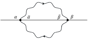
Figure 1: Second-order diagram of the resonant level Majorana fermion self-energy. The bath $\langle\psi^{\dagger}_{c}\psi_{c}\rangle$ and Majorana $\langle\gamma_{\alpha}\gamma_{\alpha}\rangle$ propagators are represented by wiggly and straight lines, respectively. Here, $\alpha=1,2$ label the two Majorana species, and we defined $\bar{\alpha}=1$ if $\alpha=2$ (and vice-versa).

III.4 Perturbative treatment around the Emery-Kivelson point

We now present perturbative results for the conductance away from the Emery-Kivelson point at order $\lambda^{2}$. A similar strategy was used previously to find thermodynamic quantities and the bulk resistivity in the two-channel Kondo context Sengupta and Georges (1994); Coleman et al. (1995); Žitko (2011). Straighforward calculations (see Appendix A) give the following correction to the $\gamma_{2}$ propagator:

$$\delta G_{\gamma_{2}\gamma_{2}}^{(2)}(\omega)=\lambda^{2}\sum_{\alpha,\beta=1,2}(-1)^{\alpha+\beta}G^{(0)}_{\gamma_{2}\gamma_{\alpha}}(\omega)\Sigma^{R}_{\bar{\alpha}\bar{\beta}}(\omega)G^{(0)}_{\gamma_{\beta}\gamma_{2}}(\omega),$$ (28)

where $\bar{\alpha}=1$ if $\alpha=2$ and vice-versa. The associated self-energy matrix (see the diagram in Fig. 1) reads

$$\Sigma^{R}_{\alpha\beta}(\omega) = \int\frac{d\omega_{1}d\omega_{2}}{\pi}\frac{(-\pi\rho^{2}\omega_{1})\text{Im}[G^{(0)}_{\gamma_{\alpha}\gamma_{\beta}}(\omega_{2})]}{\omega+i\eta-\omega_{1}-\omega_{2}}$$

$$\times\left[n_{B}(\omega_{1})+n_{F}(-\omega_{2})\right].$$

The resulting (dimensionless) second-order correction to the linear-response conductance is therefore given by

$$\delta g_{2}=\frac{\delta G_{2}}{e^{2}/h}=\int d\omega\Gamma\delta A^{(2)}_{\gamma_{2}}(\omega)\left(-\frac{\partial n_{F}(\omega)}{\partial\omega}\right),$$ (30)

where the second-order correction to the spectral density is $\delta A^{(2)}_{\gamma_{2}}(\omega)=-\text{Im}[\delta G_{\gamma_{2}\gamma_{2}}^{(2)}(\omega)]$. Eqs. (27-30) are the central results of this paper; they allow us to investigate the various scaling laws related to dissipative tunneling.

IV Analysis of the transport scaling laws

In this section, we study in detail the scaling laws, and examine three different regimes: (i) large detuning (Sec. IV.1); (ii) perfect tuning at the Majorana quantum critical point (Sec. IV.2); (iii) small detuning away from the quantum critical point (Sec. IV.3). The main question to be addressed is whether the scaling laws derived from the non-interacting Hamiltonian at the Emery-Kivelson point are modified by the perturbation of the contact interaction.

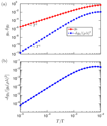
Figure 2: (color online) Large detuning, conductance shows single-barrier scaling. (a) Low-temperature behavior of the conductance $g_{0}$ at the Emery-Kivelson point (red, diamond) and the interaction-driven correction $\delta g_{2}$ (blue, circle), in the regime of sizeable detuning (here $\epsilon_{\textrm{d}}=0.1\,\Gamma$ for which $\Gamma^{\prime}\approx 0.02\,\Gamma$), as a function of $T/\Gamma$. (b) The small dimensionless ratio $-\delta g_{2}/[g_{0}(\rho\lambda)^{2}]$ indicates the validity of the single-barrier scaling in the present case.

IV.1 Large detuning: single barrier scaling

The simplest situation is that of a deep level in the quantum dot, $|\epsilon_{\textrm{d}}|\gtrsim\Gamma^{\prime}$, where $\Gamma^{\prime}$ is the low-energy renormalized width of the resonance (which can be much smaller than $\Gamma$). As a result, the electrons tunnel through the system in a single process (co-tunneling) Ingold and Nazarov (1992), with only virtual occupation of the resonant level. In this case, the backscattering operator (in the bosonization formulation) is relevant at low temperatures. The backscattering drives the system to an insulating state Kane and Fisher (1992); Furusaki and Nagaosa (1993); Eggert and Affleck (1992); Sassetti et al. (1995); Polyakov and Gornyi (2003); Bomze et al. (2009). Thus, the exact solution $g_{0}(T)$ at the Emery-Kivelson point in this situation should have the same low-temperature scaling as the conductance in tunneling through a strong single barrier Kane and Fisher (1992) in a Luttinger liquid, namely $g_{0}(T)\propto T^{2(1/g-1)}=T^{2}$ at low temperature. This was indeed verified in Ref. Komnik and Gogolin, 2003 and can be seen by performing the integral in Eq. (27) at $T\rightarrow 0$ for large detuning,

$$g_{0}\approx\int d\omega\frac{\Gamma^{2}\omega^{2}}{\epsilon_{\textrm{d}}^{4}}\frac{\beta\text{e}^{\beta\omega}}{(1+\text{e}^{\beta\omega})^{2}}=\frac{\pi^{2}}{3}\left(\frac{T}{\Gamma}\right)^{2}\left(\frac{\Gamma}{\epsilon_{\textrm{d}}}\right)^{4}.$$ (31)

The contact interaction should, for small $\lambda$, become ineffective in this limit: when the dot dynamics is frozen, the contribution of the contact interaction to $\delta g_{2}$ is irrelevant. Analyzing the asymptotic low-temperature scaling of Eq. (30), we find indeed

$$\delta g_{2}\propto-\left(\frac{T}{\Gamma}\right)^{4}\left(\frac{\Gamma}{\epsilon_{\textrm{d}}}\right)^{6}.$$ (32)

Figure 2(a) shows the results for $g_{0}$ and $\delta g_{2}$ at $\epsilon_{\textrm{d}}=0.1\,\Gamma$ after performing the numerical integrals in Eqs. (27) and (30). Although $\epsilon_{\textrm{d}}$ is not very large for this particular example, the single-barrier scaling law is already remarkably well obeyed. The observed low-temperature scaling ($\sim T^{2}$ for $g_{0}$ and $\sim T^{4}$ for $\delta g_{2}$) confirms our asymptotic analysis.

Figure 2(b) plots the ratio between $\delta g_{2}$ and $g_{0}$ normalized by the dimensionless perturbation parameter $(\rho\lambda)^{2}$, which should be less than $1$ to validate the perturbation theory. In the low-temperature regime, this ratio is much smaller than $1$ and scales to zero as $T^{2}$. Therefore, we conclude that including the contact interaction term perturbatively up to second-order does not modify the low-temperature single barrier scaling at the insulating fixed point. This finding corroborates the experimental observation Mebrahtu et al. (2013) of the applicability of single-barrier scaling Aristov and Wolfle (2008) to describe the dissipative resonant-level system away from the resonance.

IV.2 Low-temperature scaling at the conducting critical point

We now consider the case of perfect tuning to the quantum critical point $\epsilon_{\textrm{d}}=0$, and focus on the low-temperature approach to the unitary conductance Mebrahtu et al. (2012) for $T\ll\Gamma$. By solving for the exact solution at the Emery-Kivelson point ($\lambda=0$), Komnik and Gogolin Komnik and Gogolin (2003) pointed out that the approach obeys a Fermi liquid form Polyakov and Gornyi (2003), as can be checked in the considered regime from Eq. (27):

$$g_{0}=1-\int d\omega\frac{\omega^{4}}{\omega^{4}+\Gamma^{2}\omega^{2}}\frac{\beta\text{e}^{\beta\omega}}{(1+\text{e}^{\beta\omega})^{2}}\approx 1-\frac{\pi^{2}}{3}\left(\frac{T}{\Gamma}\right)^{2}.$$ (33)

This result however corresponds to an exact and unfortunate cancellation of the leading irrelevant operator Emery and Kivelson (1992); Sengupta and Georges (1994) at the conducting fixed point.

From Eq. (24), we observe that when $\epsilon_{\textrm{d}}=0$ only half of the Majorana modes (namely $\gamma_{2}$) hybrize with the leads, leaving the $\gamma_{1}$ Majorana fermion fully decoupled from the rest of the system. Including the contact interaction term $\lambda$ does not destroy the isolated Majorana mode; however, it does give rise to an anomalous non-Fermi liquid temperature dependence. In the resonant case, because the Green function between $\gamma_{1}$ and $\gamma_{2}$ vanishes [see Eq. (24a)], the only non-zero correction to the $\gamma_{2}$ propagator in Fig. 1 is

$$\delta g_{2}=\int d\omega\Gamma\left(-\text{Im}\left[\lambda^{2}\left(G^{(0)}_{\gamma_{2}\gamma_{2}}(\omega)\right)^{2}\Sigma^{R}_{11}(\omega)\right]\right)\left(-\frac{\partial n_{F}(\omega)}{\partial\omega}\right).$$ (34)

For $\epsilon_{\textrm{d}}=0$, $G^{(0)}_{\gamma_{2}\gamma_{2}}(\omega)=1/(\omega+i\Gamma)$ and $G^{(0)}_{\gamma_{1}\gamma_{1}}(\omega)=1/(\omega+i\eta)$. Hence, $\text{Im}[G^{(0)}_{\gamma_{1}\gamma_{1}}(\omega)]=-\pi\delta(\omega)$. The self-energy $\Sigma^{R}_{11}$ can be evaluated readily

$$\Sigma^{R}_{11}(\omega,\;\epsilon_{\textrm{d}}=0) = \frac{\rho^{2}}{\beta}[P_{1}(\beta\omega)+iP_{2}(\beta\omega)],$$ (35a)

$$P_{1}(\beta\omega) = \fint dx\frac{x}{\beta\omega-x}\frac{1}{2}\text{coth}\left(\frac{x}{2}\right),$$ (35b)

$$P_{2}(\beta\omega) = -\frac{\pi\beta\omega}{2}\text{coth}\left(\frac{\beta\omega}{2}\right).$$ (35c)

Plugging Eq. (35) into Eq. (34), we have

$$\delta g_{2}=(\rho\lambda)^{2}\int d\omega\left(-\frac{\Gamma}{\beta}\right)\Bigg{[}\frac{\omega^{2}-\Gamma^{2}}{(\omega^{2}+\Gamma^{2})^{2}}P_{2}(\beta\omega)\qquad\qquad\qquad$$

$$\qquad\qquad\qquad\qquad\quad-\frac{2\omega\Gamma}{(\omega^{2}+\Gamma^{2})^{2}}P_{1}(\beta\omega)\Bigg{]}\frac{\beta\text{e}^{\beta\omega}}{(1+\text{e}^{\beta\omega})^{2}}.$$ (36)

In the low-temperature limit, the $P_{2}$ part dominates, and we obtain the following asymptotic scaling for $T\ll\Gamma$:

$$\frac{\delta g_{2}}{(\rho\lambda)^{2}}\approx\int d\omega\left(-\frac{\Gamma}{\beta}\right)\frac{1}{\Gamma^{2}}\frac{\pi\beta\omega}{2}\text{coth}\left(\frac{\beta\omega}{2}\right)\frac{\beta\text{e}^{\beta\omega}}{(1+\text{e}^{\beta\omega})^{2}}=-\frac{\pi^{3}}{8}\frac{T}{\Gamma}.$$ (37)

This striking $T$ dependence is a strong signature of the uncoupled Majorana mode $\gamma_{1}$. Indeed, on resonance $\epsilon_{\textrm{d}}=0$, the correlation function of $\gamma_{1}$ does not decay at long time, $G_{\gamma_{1}\gamma_{1}}(t)=-\langle\gamma_{1}(0)\gamma_{1}(t)\rangle\propto 1$, instead of the usual $1/t$ decay for hybridized modes. This translates into a $1/t^{2}$ decay of the $\gamma_{2}$ self-energy correction (instead of $1/t^{3}$ for a usual Fermi liquid), giving rise by Fourier transform to a linear in frequency scattering rate. This linear approach to the unitary conductance signals the presence of an isolated Majorana state Sengupta and Georges (1994); Coleman et al. (1995); Žitko (2011), and has been observed in a recent experiment Mebrahtu et al. (2013).

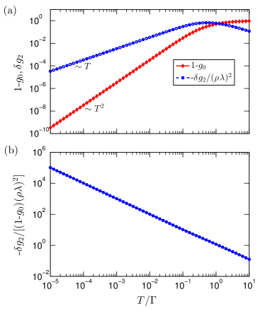
Figure 3: (color online) Approach to the quantum critical point; here $\epsilon_{\textrm{d}}=0$. (a) Low-temperature behavior of $1-g_{0}$ (red, diamond) and $\delta g_{2}$ (blue, circle) close to the conducting quantum critical point. (b) The scaling of $-\delta g_{2}/[(1-g_{0})(\rho\lambda)^{2}]$ as a function of $T/\Gamma$ shows that the interaction correction dominates.

Figure 3(a) shows both $1\!-\!g_{0}$ and $\delta g_{2}$ obtained by numerical integration. The asymptotic scalings are reproduced at low temperatures. Figure 3(b) plots the ratio of $-\delta g_{2}$ to $1-g_{0}$ normalized by the dimensionless perturbation parameter $(\rho\lambda)^{2}$. As long as $(\rho\lambda)^{2}$ is not too small, the linear temperature scaling strongly dominates over the quadratic behavior as $T\!\rightarrow\!0$. Hence, we conclude that the contact interaction between the Majorana modes and the effective leads generates non-Fermi liquid behavior at the Majorana quantum critical point.

Note that the four-fermion interaction term in Eq. (II.3) is too large ($\lambda=\pi v_{F}$) for the perturbation theory to quantitatively capture the full crossover from high temperature ($T\gg\Gamma^{\prime}$) to the asymptotic non-Fermi liquid regime ($T\ll\Gamma^{\prime}$), where $\Gamma^{\prime}\ll\Gamma$ is the strongly renormalized linewidth. This strong coupling regime Žitko and Simon (2011) leads to universal scaling relations describing the full crossover towards the quantum critical state in our system.

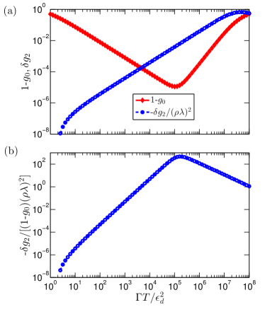
Figure 4: (color online) Small detuning, the runaway flow. Here, we choose $\epsilon_{\textrm{d}}=10^{-4}\Gamma$. (a) $1-g_{0}$ (red, diamond) and $\delta g_{2}$ (blue, circle) as a function of $\Gamma T/\epsilon_{\textrm{d}}^{2}$. (b) The ratio $-\delta g_{2}/[(1-g_{0})(\rho\lambda)^{2}]$ as a function of $\Gamma T/\epsilon_{\textrm{d}}^{2}$. Initially, the interaction corrections dominate as one approaches the critical point, but then the system veers away toward the insulating fixed point and the non-interacting term, $g_{0}$, dominates in the end.

IV.3 Small detuning: runaway flow

We finally investigate intermediate-temperature scaling with a slight detuning from the quantum critical point, $T\ll\epsilon_{d}\ll\sqrt{T\Gamma}$. In that regime, the renormalization flow approaches very close to the conducting fixed point, but ultimately flows away from it because the transparency is not perfectly unity. Considering first the Emery-Kivelson solution Eq. (27) in this limit, we obtain the runaway behavior from the unitary conductance, which has the same $1/T$ temperature dependence as tunneling through a weak single barrier Kane and Fisher (1992); Komnik and Gogolin (2003):

$$g_{0} = 1-\int d\omega\frac{(\omega^{2}-\epsilon_{\textrm{d}}^{2})^{2}}{(\omega^{2}-\epsilon_{\textrm{d}}^{2})^{2}+\Gamma^{2}\omega^{2}}\frac{\beta\text{e}^{\beta\omega}}{(1+\text{e}^{\beta\omega})^{2}}\qquad\qquad$$ (38)

$$\approx 1- \int d\omega\frac{(\epsilon_{\textrm{d}}^{2}/\Gamma)^{2}}{\omega^{2}+(\epsilon_{\textrm{d}}^{2}/\Gamma)^{2}}\frac{\beta\text{e}^{\beta\omega}}{(1+\text{e}^{\beta\omega})^{2}}$$

$$\approx 1- \int d\omega\frac{(\epsilon_{\textrm{d}}^{2}/\Gamma)^{2}}{\omega^{2}+(\epsilon_{\textrm{d}}^{2}/\Gamma)^{2}}\frac{\beta\text{e}^{0}}{(1+\text{e}^{0})^{2}}=1-\frac{\pi}{4}\left(\frac{\epsilon_{\textrm{d}}^{2}}{\Gamma T}\right).$$

In Eq. (38), we used in the second and third lines the conditions $\Gamma\gg\epsilon_{\textrm{d}}\gg T$ and $T\gg\epsilon_{\textrm{d}}^{2}/\Gamma$, respectively.

On the other hand, $\delta g_{2}$ still obeys Eq. (37), since $\Gamma\gg\epsilon_{\textrm{d}}$, $T$. Therefore, we have the ratio

$$-\frac{\delta g_{2}}{1-g_{0}}\approx\frac{\pi^{2}}{2}(\rho\lambda)^{2}\left(\frac{T}{\epsilon_{\textrm{d}}}\right)^{2},$$ (39)

which is much smaller than $1$ for $T\ll\epsilon_{\textrm{d}}$, indicating that the runaway flow of $1-g_{0}$ is not modified by the perturbation correction from the contact interaction term.

Figure 4(a) presents $1-g_{0}$ and $\delta g_{2}$ as a function of $\Gamma T/\epsilon_{\textrm{d}}^{2}$ with a small detuning $\epsilon_{\textrm{d}}=10^{-4}\Gamma$ over a wide temperature range. For very low temperature $T\sim\epsilon_{\textrm{d}}^{2}/\Gamma$, $1-g_{0}\sim 1$ showing that even a small detuning can drive the system to the insulating critical point with a vanishing conductance. In the intermediate-temperature regime ($10^{1}\lesssim\Gamma T/\epsilon_{\textrm{d}}^{2}\lesssim 10^{3}$), the condition $\Gamma\gg\epsilon_{\textrm{d}}\gg T\gg\epsilon_{\textrm{d}}^{2}/\Gamma$ is satisfied. Clearly, Fig. 4(b) shows that in this temperature range $\delta g_{2}$ is subdominant compared to $1-g_{0}$. Further increase of temperature leads to the regime $\Gamma\gg T\gtrsim\epsilon_{\textrm{d}}$ ($10^{4}\lesssim\Gamma T/\epsilon_{\textrm{d}}^{2}\lesssim 10^{7}$). In this regime, $1-g_{0}$ changes from $1/T$ to $T^{2}$ dependence and $\delta g_{2}$ starts to dominate the runaway scaling as shown in Fig. 4(b).

To conclude this study, we give in Table 1 a summary of the scalings in the three different regimes discussed in this section. The contact interaction controls the approach to the quantum critical point, but is strongly irrelevant otherwise, leading to effectively single barrier scaling.

Regime	$g_{0}$	$1-g_{0}$	$-\delta g_{2}/(\rho\lambda)^{2}$
$\epsilon_{\textrm{d}}\sim\Gamma\gg T$	$\displaystyle\sim\frac{\pi^{2}}{3}\left(\frac{T}{\Gamma}\right)^{2}\left(\frac{\Gamma}{\epsilon_{\textrm{d}}}\right)^{4}$	$\sim 1$	$\displaystyle\propto\left(\frac{T}{\Gamma}\right)^{4}\left(\frac{\Gamma}{\epsilon_{\textrm{d}}}\right)^{6}$
$\epsilon_{\textrm{d}}=0$, $\Gamma\gg T$	$\sim 1$	$\displaystyle\sim\frac{\pi^{2}}{3}\left(\frac{T}{\Gamma}\right)^{2}$	$\displaystyle\sim\frac{\pi^{3}}{8}\left(\frac{T}{\Gamma}\right)$
$\displaystyle\Gamma\gg\epsilon_{\textrm{d}}\gg T\gg\frac{\epsilon_{\textrm{d}}^{2}}{\Gamma}$	$\sim 1$	$\displaystyle\sim\frac{\pi}{4}\left(\frac{\epsilon_{\textrm{d}}^{2}}{\Gamma T}\right)$	$\displaystyle\sim\frac{\pi^{3}}{8}\left(\frac{T}{\Gamma}\right)$

Table 1: Summary of various low-temperature scalings close to the insulating and conducting fixed points. The first, second, and third rows correspond to large detuning, exactly critical tuning, and small detuning (runaway flow), respectively.

V Conclusion

In summary, we have studied spinless resonant tunneling with a large, fine-tuned circuit impedance $R=e^{2}/h$ and mapped it directly to resonant tunneling between Luttinger liquids with Luttinger parameter $g=1/2$. We further mapped the system to a resonant Majorana model in the case of symmetric coupling. In contrast to previous studies, we retained the contact interaction between the resonant level and the leads. Perturbation theory of the linear-response conductance is developed up to second-order in the contact interaction. We found that while the second-order correction does not change the single-barrier scaling near the insulating fixed point, it does give rise to a linear temperature dependence as the conductance approaches unity when the resonant level is tuned to be exactly on resonance (Majorana quantum critical point). This striking non-Fermi liquid behavior is due to the fact that the resonant level is fractionalized into two independent Majorana fermions, with one of them fully isolated from the rest of the system. Further investigations could, for instance, concentrate on incorporating the spin degree of freedom on the quantum dot, leading to a rich interplay of Luttinger and Kondo physics.

Appendix A Derivation of the self-energy correction

The diagrammatic calculations proceed by expanding the propagator of the $\gamma_{2}$ Majorana mode in powers of the contact interaction term $H_{C}$:

$$G_{\gamma_{2}\gamma_{2}}(\tau) = -\langle T_{\tau}\gamma_{2}(\tau)\gamma_{2}(0)\rangle$$

$$= -\Big{\langle}T_{\tau}\Big{\{}\gamma_{2}(\tau)\gamma_{2}(0)\text{exp}\Big{[}-\int^{\beta}_{0}d\tau H_{C}(\tau)\Big{]}\Big{\}}\Big{\rangle}_{0}$$

$$= -\sum_{n}\Big{\langle}T_{\tau}\Big{\{}\gamma_{2}(\tau)\gamma_{2}(0)\frac{1}{n!}\Big{[}-{\textstyle\int}d\tau^{\prime}H_{C}(\tau^{\prime})\Big{]}^{n}\Big{\}}\Big{\rangle}_{0}.$$

The zeroth-order contribution provides the non-interacting contribution already given in the conductance formula (27). The first-order contribution vanishes due to a disconnected diagram of the $\psi_{c}$ field under the non-interacting Hamiltonian. We therefore focus on the second-order contribution, which gives rise to a correction to the spectral function in Eq. (25) and hence to a correction to the linear response conductance. The diagram for the second-order perturbation is shown in Fig. 1 and reads

$$\!\!\!\delta G_{\gamma_{2}\gamma_{2}}^{(2)}(\tau) = \frac{\lambda^{2}}{2}\!\!\iint\!\!\!\!d\tau_{1}d\tau_{2}\Big{\langle}T_{\tau}\Big{[}\!\colon\psi^{\dagger}_{c}(\tau_{1})\psi_{c}(\tau_{1})\psi^{\dagger}_{c}(\tau_{2})\psi_{c}(\tau_{2})\colon\!\Big{]}\Big{\rangle}_{0}$$

$$\times\Big{\langle}T_{\tau}\Big{[}\gamma_{2}(\tau)\gamma_{2}(0)\gamma_{1}(\tau_{1})\gamma_{2}(\tau_{1})\gamma_{1}(\tau_{2})\gamma_{2}(\tau_{2})\Big{]}\Big{\rangle}_{0}$$

$$= \lambda^{2}\iint d\tau_{1}d\tau_{2}\sum_{\alpha,\beta=1,2}(-1)^{\alpha+\beta}G^{(0)}_{\gamma_{2}\gamma_{\alpha}}(\tau-\tau_{1})$$

$$\times\Sigma_{\bar{\alpha}\bar{\beta}}(\tau_{1}-\tau_{2})G{(0)}_{\gamma_{\beta}\gamma_{2}}(\tau_{2}),$$

where $\bar{\alpha}=1$ if $\alpha=2$ (and vice-versa).

The self-energy of Majorana fermions is defined as

$$\Sigma_{\alpha\beta}(\tau)=G^{(0)}_{c}(\tau)G^{(0)}_{c}(-\tau)G^{(0)}_{\gamma_{\alpha}\gamma_{\beta}}(\tau),$$ (42a)

$$G^{(0)}_{c}(\tau)=-\langle T_{\tau}\psi^{\dagger}_{c}(x=0,\tau)\psi_{c}(x=0,0)\rangle_{0}.$$ (42b)

After Fourier transformation of Eqs. (A) and (42), we have

$$\delta G_{\gamma_{2}\gamma_{2}}^{(2)}(i\omega_{n}) = \!\lambda^{2}\!\!\!\sum_{\alpha,\beta=1,2}\!\!\!(-1)^{\alpha+\beta}G^{(0)}_{\gamma_{2}\gamma_{\alpha}}(i\omega_{n})\Sigma_{\bar{\alpha}\bar{\beta}}(i\omega_{n})G^{(0)}_{\gamma_{\beta}\gamma_{2}}(i\omega_{n}),$$

$$\Sigma_{\alpha\beta}(i\omega_{n}) = \frac{1}{\beta}\sum_{ip_{n}}\,\chi(ip_{n})\,G^{(0)}_{\gamma_{\alpha}\gamma_{\beta}}(i\omega_{n}-ip_{n}),$$ (43b)

$$\chi(ip_{n}) = \frac{1}{\beta}\sum_{iq_{n}}G^{(0)}_{c}(ip_{n}+iq_{n})\,G^{(0)}_{c}(iq_{n}).$$ (43c)

Here, $p_{n}$ and $q_{n}$ are bosonic and fermionic Matsubara frequencies, respectively. The Matsubara sum over $iq_{n}$ can be done easily, since $G^{(0)}_{c}(iq_{n})$ has a simple pole Bruus and Flensberg (2004); Mahan (1979), so that:

$$\chi(ip_{n}) = \int d\epsilon_{1}d\epsilon_{2}\frac{1}{\beta}\sum_{iq_{n}}\frac{\rho}{iq_{n}+\epsilon_{1}}\frac{\rho}{ip_{n}+iq_{n}+\epsilon_{2}}$$

$$= \int d\epsilon_{1}d\epsilon_{2}\frac{\rho^{2}}{ip_{n}+\epsilon_{1}-\epsilon_{2}}\left[n_{F}(\epsilon_{1})-n_{F}(\epsilon_{2})\right].$$

To evaluate the self-energy, we rely on the following identity of Matsubara Green functions Mahan (1979)

$$G(i\omega_{n})=-\int\frac{d\epsilon}{\pi}\frac{\text{Im}[G^{R}(\epsilon)]}{i\omega_{n}-\epsilon}.$$ (45)

Using this, Eq. (43b) can be written as

$$\Sigma_{\alpha\beta}(i\omega_{n}) = \frac{1}{\beta}\sum_{ip_{n}}\frac{\int d\omega_{1}d\omega_{2}}{\pi^{2}}\frac{\text{Im}[\chi^{R}(\omega_{1})]}{ip_{n}-\omega_{1}}\frac{\text{Im}[G^{(0)}_{\gamma_{\alpha}\gamma_{\beta}}(\omega_{2})]}{i\omega_{n}-ip_{n}-\omega_{2}}$$

$$= \int\frac{d\omega_{1}d\omega_{2}}{\pi}\frac{\text{Im}[\chi^{R}(\omega_{1})]\text{Im}[G^{(0)}_{\gamma_{\alpha}\gamma_{\beta}}(\omega_{2})]}{i\omega_{n}-\omega_{1}-\omega_{2}}$$

$$\times\left[n_{B}(\omega_{1})+n_{F}(-\omega_{2})\right],$$

where $n_{B}$ is the Bose-Einstein distribution function. Again, the summation over $ip_{n}$ is straightforward because the integrand has only two simple poles at $\omega_{1}$ and $i\omega_{n}-\omega_{2}$ Mahan (1979). Performing an analytic continuation and evaluating the integral in Eq. (A), we obtain $\text{Im}[\chi^{R}(\omega)]=-\pi\rho^{2}\omega$ in the wide band limit. After analytic continuation of Eq. (43a) and Eq. (A), we arrive at Eqs. (28)-(III.4) quoted in the main text.

References

- Chang (2003) A. M. Chang, Reviews Of Modern Physics 75, 1449 (2003).
- Deshpande et al. (2010) V. V. Deshpande, M. Bockrath, L. I. Glazman, and A. Yacoby, Nature 464, 209 (2010).
- Blumenstein et al. (2011) C. Blumenstein, J. Schäfer, S. Mietke, S. Meyer, A. Dollinger, M. Lochner, X. Y. Cui, L. Patthey, R. Matzdorf, and R. Claessen, Nat. Phys. 7, 776 (2011).
- Laroche et al. (2014) D. Laroche, G. Gervais, M. P. Lilly, and J. L. Reno, Science 343, 631 (2014), http://www.sciencemag.org/content/343/6171/631.full.pdf .
- Roch et al. (2009) N. Roch, S. Florens, T. A. Costi, W. Wernsdorfer, and F. Balestro, Phys. Rev. Lett. 103, 197202 (2009).
- Florens et al. (2011) S. Florens, A. Freyn, N. Roch, W. Wernsdorfer, F. Balestro, P. Roura-Bas, and A. A. Aligia, J. Phys. Cond. Mat. 23, 243202 (2011).
- Grobis et al. (2007) M. Grobis, I. G. Rau, R. M. Potok, and D. Goldhaber-Gordon, in Handbook of Magnetism and Advanced Magnetic Materials, Vol. 5, edited by H. Kronmüller and S. Parkin (Wiley, 2007) pp. 2703–2724, arXiv:cond-mat/0611480.
- Potok et al. (2007) R. M. Potok, I. G. Rau, H. Shtrikman, Y. Oreg, and D. Goldhaber-Gordon, Nature 446, 167 (2007).
- Parmentier et al. (2011) F. D. Parmentier, A. Anthore, S. Jezouin, H. l. Sueur, U. Gennser, A. Cavanna, D. Mailly, and F. Pierre, Nat Phys 7, 935 (2011).
- Mebrahtu et al. (2012) H. T. Mebrahtu, I. V. Borzenets, D. E. Liu, H. Zheng, Y. V. Bomze, A. I. Smirnov, H. U. Baranger, and G. Finkelstein, Nature 488, 61 (2012).
- Mebrahtu et al. (2013) H. T. Mebrahtu, I. V. Borzenets, H. Zheng, Y. V. Bomze, A. I. Smirnov, S. Florens, H. U. Baranger, and G. Finkelstein, Nat. Phys. 9, 732 (2013).
- Jezouin et al. (2013) S. Jezouin, M. Albert, F. D. Parmentier, A. Anthore, U. Gennser, A. Cavanna, I. Safi, and F. Pierre, Nat. Comm. 4, 1802 (2013).
- Giamarchi (2004) T. Giamarchi, Quantum Physics in One Dimension (Oxford University Press, New York, 2004).
- Safi and Saleur (2004) I. Safi and H. Saleur, Phys. Rev. Lett. 93, 126602 (2004).
- Florens et al. (2007) S. Florens, P. Simon, S. Andergassen, and D. Feinberg, Phys. Rev. B 75, 155321 (2007).
- Komnik and Gogolin (2003) A. Komnik and A. O. Gogolin, Phys. Rev. Lett. 90, 246403 (2003).
- Ingold and Nazarov (1992) G.-L. Ingold and Y. Nazarov, in Single Charge Tunneling: Coulomb Blockade Phenomena in Nanostructures, edited by H. Grabert and M. H. Devoret (Plenum, New York, 1992) pp. 21–107.
- Yu. V. Nazarov and Blanter (2009) Yu. V. Nazarov and Y. M. Blanter, Quantum Transport: Introduction to Nanoscience (Cambridge University Press, Cambridge, 2009) p. 499.
- Imam et al. (1994) H. T. Imam, V. V. Ponomarenko, and D. V. Averin, Phys. Rev. B 50, 18288 (1994).
- Cedraschi et al. (2000) P. Cedraschi, V. V. Ponomarenko, and M. Büttiker, Phys. Rev. Lett. 84, 346 (2000).
- Le Hur (2004) K. Le Hur, Phys. Rev. Lett. 92, 196804 (2004).
- Le Hur and Li (2005) K. Le Hur and M.-R. Li, Phys. Rev. B 72, 073305 (2005).
- Borda et al. (2005) L. Borda, G. Zaránd, and P. Simon, Phys. Rev. B 72, 155311 (2005).
- Borda et al. (2006) L. Borda, G. Zaránd, and D. Goldhaber-Gordon, eprint arXiv:cond-mat/0602019 (2006).
- Glossop and Ingersent (2007) M. T. Glossop and K. Ingersent, Phys. Rev. B 75, 104410 (2007).
- Chung et al. (2007) C.-H. Chung, M. T. Glossop, L. Fritz, M. Kirćan, K. Ingersent, and M. Vojta, Phys. Rev. B 76, 235103 (2007).
- Cheng et al. (2009) M. Cheng, M. T. Glossop, and K. Ingersent, Phys. Rev. B 80, 165113 (2009).
- Liu et al. (2014) D. E. Liu, H. Zheng, G. Finkelstein, and H. U. Baranger, Phys. Rev. B 89, 085116 (2014).
- Caldeira and Leggett (1981) A. O. Caldeira and A. J. Leggett, Phys. Rev. Lett. 46, 211 (1981).
- Leggett et al. (1987) A. J. Leggett, S. Chakravarty, A. T. Dorsey, M. P. A. Fisher, A. Garg, and W. Zwerger, Rev. Mod. Phys. 59, 1 (1987).
- Kane and Fisher (1992) C. L. Kane and M. P. A. Fisher, Phys. Rev. B 46, 15233 (1992).
- Furusaki and Nagaosa (1993) A. Furusaki and N. Nagaosa, Phys. Rev. B 47, 3827 (1993).
- Eggert and Affleck (1992) S. Eggert and I. Affleck, Phys. Rev. B 46, 10866 (1992).
- Emery and Kivelson (1992) V. J. Emery and S. Kivelson, Phys. Rev. B 46, 10812 (1992).
- Fabrizio and Gogolin (1995) M. Fabrizio and A. O. Gogolin, Phys. Rev. B 51, 17827 (1995).
- Goldstein and Berkovits (2010) M. Goldstein and R. Berkovits, Phys. Rev. B 82, 161307 (2010).
- (37) I. Affleck, private communication.
- Wong and Affleck (1994) E. Wong and I. Affleck, Nucl. Phys. B 417, 403 (1994).
- Sengupta and Georges (1994) A. M. Sengupta and A. Georges, Phys. Rev. B 49, 10020 (1994).
- Coleman et al. (1995) P. Coleman, L. B. Ioffe, and A. M. Tsvelik, Phys. Rev. B 52, 6611 (1995).
- Žitko (2011) R. Žitko, Phys. Rev. B 83, 195137 (2011).
- Bruus and Flensberg (2004) H. Bruus and K. Flensberg, Many-body quantum theory in condensed matter physics: an introduction (Oxford Univ. Press, 2004).
- Maslov and Stone (1995) D. L. Maslov and M. Stone, Phys. Rev. B 52, R5539 (1995).
- Safi and Schulz (1995) I. Safi and H. J. Schulz, Phys. Rev. B 52, 17040 (1995).
- Ponomarenko (1995) V. V. Ponomarenko, Phys. Rev. B 52, 8666 (1995).
- Meir and Wingreen (1992) Y. Meir and N. S. Wingreen, Phys. Rev. Lett. 68, 2512 (1992).
- Sassetti et al. (1995) M. Sassetti, F. Napoli, and U. Weiss, Phys. Rev. B 52, 11213 (1995).
- Polyakov and Gornyi (2003) D. G. Polyakov and I. V. Gornyi, Phys. Rev. B 68, 035421 (2003).
- Bomze et al. (2009) Y. Bomze, H. Mebrahtu, I. Borzenets, A. Makarovski, and G. Finkelstein, Phys. Rev. B 79, 241402 (2009).
- Aristov and Wolfle (2008) D. N. Aristov and P. Wolfle, EPL 82, 27001 (2008).
- Žitko and Simon (2011) R. Žitko and P. Simon, Phys. Rev. B 84, 195310 (2011).
- Mahan (1979) G. D. Mahan, Many-Particle Physics, 2nd ed. (Springer, 1979).