Dicke superradiance as a nondestructive probe for quantum quenches in optical lattices

Abstract

We study Dicke superradiance as collective and coherent absorption and (time-delayed) emission of photons from an ensemble of ultracold atoms in an optical lattice. Since this process depends on the coherence properties of the atoms (e.g., superfluidity), it can be used as a probe for their quantum state. In analogy to pump-probe spectroscopy in solid-state physics, this detection method facilitates the investigation of nonequilibrium phenomena and is less invasive than time-of-flight experiments or direct (projective) measurements of the atom number (or parity) per lattice site, which both destroy properties of the quantum state such as phase coherence.

I Introduction

Ultracold atoms in optical lattices are very nice tools for investigating quantum many-body physics since they can be well isolated from the environment and cooled down to very low temperatures Raizen et al. (1997); Bloch (2004, 2005). Furthermore, it is possible to control these systems and to measure their properties to a degree which cannot be reached in many other scenarios. For example, the quantum phase transition Sachdev (2011) between the highly correlated Mott insulator state and the superfluid phase in the Bose-Hubbard model Fisher et al. (1989); Jaksch et al. (1998); Jaksch and Zoller (2005) has been observed Greiner et al. (2002); Stöferle et al. (2004); Spielman et al. (2007). This observation was accomplished by time-of-flight experiments where the optical lattice trapping the atoms is switched off and their positions are measured after a waiting time. As another option for detecting the state of the atoms, the direct in situ measurement of the number of atoms per lattice site (or more precisely, the parity) has been achieved recently (see, e.g., Sherson et al. (2010); Endres et al. (2013)). However, both methods are quite invasive since they destroy properties of the quantum state such as phase coherence.

Methods for less destructive probing of the quantum state of atoms in optical lattices were proposed recently, e.g., the interaction with light in an optical cavity Landig et al. (2015); Rajaram and Trivedi (2013); Silver et al. (2010); Bhaseen et al. (2009); Zoubi and Ritsch (2009); Chen et al. (2007); Mekhov:2007 or matter-wave scattering with (slow) atoms Sanders et al. (2010); Mayer et al. (2014). In this paper, we study an alternative, nondestructive detection method based on Dicke superradiance, i.e., the (free-space) collective and coherent absorption and emission of photons from an ensemble of ultracold atoms (see, e.g., Dicke (1954); Rehler and Eberly (1971); Lipkin (2002); Wiegner et al. (2011)). We investigate how the lattice dynamics (e.g., hopping) occurring between the absorption and subsequent superradiant emission of single photons Scully et al. (2006); Scully (2007); de Oliveira et al. (2014) changes the emission characteristics.

To probe the quantum state of the optical lattice, we envisage the following sequence (see Fig. 1): First, an infrared photon is absorbed by one of the atoms, but we do not know which one (creating a “timed” Dicke state Scully et al. (2006); Scully (2007); de Oliveira et al. (2014)). Then, during a waiting period $\Delta t$, the atoms have time to tunnel and to interact. Afterwards, the excited atoms decay back to their ground state by collectively emitting an infrared photon – depending on the coherence properties of the atoms. Options for experimental realizations will be discussed below.

II Basic Formalism

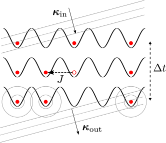
Figure 1: (Color online) Envisaged probing sequence. First, an infrared photon $\mbox{\boldmath$\kappa$}_{\rm in}$ is absorbed collectively by the ground-state atoms at their respective lattice sites. Second, the atoms tunnel and interact according to (1) during a waiting period $\Delta t$, thereby possibly compromising the spatial phase coherence of the Dicke state. In the third step, the photon is (collectively) emitted again with the wave vector $\mbox{\boldmath$\kappa$}_{\rm out}$.

Under appropriate conditions, bosonic ultracold atoms in optical lattices are approximately described by the Bose-Hubbard Hamiltonian Jaksch and Zoller (2005),

$$\hat{H}_{\rm BH}=-\frac{J}{Z}\sum_{\mu\nu}T_{\mu\nu}\hat{b}_{\mu}^{\dagger}\hat{b}_{\nu}+\frac{U}{2}\sum_{\mu}\hat{n}_{\mu}^{(b)}(\hat{n}_{\mu}^{(b)}-1)\,,$$ (1)

with the hopping rate $J$, the interaction strength $U$, the adjacency matrix $T_{\mu\nu}$, and the coordination number $Z$. Here, we assume a quadratic lattice with $Z=4$. Furthermore, $\hat{b}_{\mu}^{\dagger}$ and $\hat{b}_{\nu}$ denote the creation and annihilation operators of the atoms (in their ground state) at lattice sites $\mu$ and $\nu$, respectively, and $\hat{n}_{\mu}^{(b)}=\hat{b}_{\mu}^{\dagger}\hat{b}_{\mu}$ is the number operator. Assuming unit filling $\langle\hat{n}_{\mu}^{(b)}\rangle=1$, this model displays a quantum phase transition Sachdev (2011) between the superfluid phase where $J$ dominates and the Mott insulator state where $U$ dominates. In the extremal limits $J\gg U$ and $U\gg J$, the ground states simply read

$$\left|\Psi\right>_{\rm Mott}^{J=0}=\prod\limits_{\mu}\hat{b}_{\mu}^{\dagger}\left|0\right>=\bigotimes\limits_{\mu}\left|1\right>_{\mu}\,,$$ (2)

for the Mott insulator state and

$$\left|\Psi\right>_{\rm superfluid}^{U=0}=\frac{1}{\sqrt{N!}}\left(\hat{b}_{\mbox{\boldmath$\scriptstyle k$}=0}^{\dagger}\right)^{N}\left|0\right>\propto\left(\sum\limits_{\mu}\hat{b}_{\mu}^{\dagger}\right)^{N}\left|0\right>\,,$$ (3)

for the superfluid phase, where $N$ is the total number of lattice sites (which equals the number of particles).

Now, we consider the interaction of these atoms with infrared photons. Assuming that the wavelength of these infrared photons is much larger than the lattice spacing of the optical lattice, we have a large number of atoms within one (infrared) photon wavelength. In addition, the atomic recoil due to the absorption or emission of an infrared photon is negligible, which is another basic requirement for Dicke superradiance. The interaction between atoms and photons is then described by

$$\hat{H}_{\rm int}=\int d^{3}k\,g_{\mbox{\boldmath$\scriptstyle k$}}(t)\hat{a}_{\mbox{\boldmath$\scriptstyle k$}}\sum_{\mu}\hat{c}_{\mu}^{\dagger}\hat{b}_{\mu}\exp\left(i\mbox{\boldmath$k$}\cdot\mbox{\boldmath$r$}_{\mu}\right)+{\rm H.c.},$$ (4)

where $\hat{a}_{\mbox{\boldmath$\scriptstyle k$}}$ is the annihilation operator of a photon with wave number $k$ and $\mbox{\boldmath$r$}_{\mu}$ is the position of the atom at the lattice site $\mu$. The excited atoms at lattice sites $\mu$ and $\nu$ are described by the creation and annihilation operators $\hat{c}_{\mu}^{\dagger}$ and $\hat{c}_{\nu}$ and thus one has to extend the Bose-Hubbard Hamiltonian (1) accordingly.

III Emission Probability

In lowest-order perturbation theory, the probability (density) to first absorb a photon with wave number $\mbox{\boldmath$\kappa$}_{\rm in}$ and later (after the waiting time $\Delta t$) emit a photon with wave-number $\mbox{\boldmath$\kappa$}_{\rm out}$ reads

$$P = \int dt_{1}\,dt_{2}\,dt_{3}\,dt_{4}\,g_{\rm out}(t_{4})g_{\rm out}^{*}(t_{2})g_{\rm in}^{*}(t_{3})g_{\rm in}(t_{1})$$ (5)

$$\times\exp\left\{i(\omega_{\rm in}t_{3}-\omega_{\rm out}t_{4})-i(\omega_{\rm in}t_{1}-\omega_{\rm out}t_{2})\right\}$$

$$\times\mathcal{D}\left(t_{1},t_{2},t_{3},t_{4}\right)\,,$$

with the operatorial part containing the lattice dynamics

$$\mathcal{D}\left(t_{1},t_{2},t_{3},t_{4}\right)=\sum_{\mu\nu\rho\eta}\exp\left\{i\left(\mbox{\boldmath$\kappa$}_{\rm out}\cdot\mbox{\boldmath$r$}_{\rho}-\mbox{\boldmath$\kappa$}_{\rm in}\cdot\mbox{\boldmath$r$}_{\eta}\right)\right\}$$

$$\times\exp\left\{-i\left(\mbox{\boldmath$\kappa$}_{\rm out}\cdot\mbox{\boldmath$r$}_{\mu}-\mbox{\boldmath$\kappa$}_{\rm in}\cdot\mbox{\boldmath$r$}_{\nu}\right)\right\}$$

$$\times\langle\hat{b}_{\eta}^{\dagger}(t_{3})\hat{c}_{\eta}(t_{3})\hat{c}_{\rho}^{\dagger}(t_{4})\hat{b}_{\rho}(t_{4})\hat{b}_{\mu}^{\dagger}(t_{2})\hat{c}_{\mu}(t_{2})\hat{c}_{\nu}^{\dagger}(t_{1})\hat{b}_{\nu}(t_{1})\rangle.$$ (6)

The expectation value in the last line should be taken in the initial state, which could be a pure state, such as the superfluid state (3) or the Mott state (2), or a mixed state such as a thermal density matrix.

As a result, this probability (density) depends on the above four-times eight-point function, which contains information about the underlying state. Unfortunately, since the Bose-Hubbard model is not integrable, we do not have an explicit solution for this eight-point function apart from some limiting cases. Let us first study the special case that the initial state $\hat{\varrho}^{\rm in}$ contains no correlations and zero ($\hat{c}_{\mu}^{\dagger}$) excitations, i.e., it can be represented by a product of single-site states $\hat{\varrho}^{\rm in}=\otimes_{\mu}\hat{\varrho}^{\rm in}_{\mu}$ with $\langle\hat{c}_{\mu}^{\dagger}\hat{c}_{\nu}\rangle=0$. Furthermore, we assume that the correlations which arise through the time evolution $\Delta t$ remain negligible. Then, the operatorial part reads to leading order in $N$,

$$\mathcal{D}_{\mbox{\boldmath$\scriptstyle\kappa$}_{\rm out}}^{\mbox{\boldmath$\scriptstyle\kappa$}_{\rm in}}\left(t,t^{\prime}\right)=\Big{|}\sum_{\mu}\exp\left\{-i\left(\mbox{\boldmath$\kappa$}_{\rm out}-\mbox{\boldmath$\kappa$}_{\rm in}\right)\cdot\mbox{\boldmath$r$}_{\mu}\right\}\times\\ \times\langle\hat{b}_{\mu}^{\dagger}(t^{\prime})\hat{c}_{\mu}(t^{\prime})\hat{c}_{\mu}^{\dagger}(t)\hat{b}_{\mu}(t)\rangle\Big{|}^{2}\,,$$ (7)

where $t=t_{1/3}$ denotes the time when the photon is absorbed and $t^{\prime}=t_{2/4}$ the emission time. The result is quite intuitive, as the above expectation value is just the probability amplitude that the excited atom stays at the lattice site $\mu$ during the waiting time $\Delta t=t^{\prime}-t$. In the limit of $J=0$, the atoms are pinned to their lattice sites and we get the usual Dicke superradiance. In this case, the expectation value gives the number $n_{\mu}$ of atoms at site $\mu$, and the sum can be interpreted as a discrete Fourier transform of the $n_{\mu}$-distribution of the atoms in the lattice. Considering, e.g., the Mott state (2), where all the atoms are equally distributed, the Fourier transform yields a sharp peak $\delta(\mbox{\boldmath$\kappa$}_{\rm in},\mbox{\boldmath$\kappa$}_{\rm out})$, which corresponds to the well-known directed spontaneous (superradiant) emission for fixed atoms Scully et al. (2006); Scully (2007); de Oliveira et al. (2014). However, we would like to stress again that Eq. (7) is only valid when the correlations between lattice sites are negligible. Turning this argument around, a deviation from Eq. (7) is an indicator for correlations.

In the other limiting case $U=0$, we may also simplify Eq. (III). Assuming that there are no excited atoms initially $\langle\hat{c}_{\mu}^{\dagger}\hat{c}_{\nu}\rangle=0$, the eight-point function in (III) can be reduced to a four-point function in terms of the operators $\hat{b}_{\mu}^{\dagger}$ and $\hat{b}_{\nu}$. After a Fourier transform, this four-point function $\langle\hat{b}_{\mbox{\boldmath$\scriptstyle q$}-\mbox{\boldmath$\scriptstyle\kappa$}_{\rm in}}^{\dagger}\hat{b}_{\mbox{\boldmath$\scriptstyle q$}-\mbox{\boldmath$\scriptstyle\kappa$}_{\rm out}}\hat{b}_{\mbox{\boldmath$\scriptstyle p$}-\mbox{\boldmath$\scriptstyle\kappa$}_{\rm out}}^{\dagger}\hat{b}_{\mbox{\boldmath$\scriptstyle p$}-\mbox{\boldmath$\scriptstyle\kappa$}_{\rm in}}\rangle$ depends on two wave numbers $p$ and $q$ (assuming translational invariance). If we have a Gaussian state (for $U=0$), such as a thermal state or (to a very good approximation) the superfluid state (3), it can be expanded into a sum of products of two-point functions via the Wick theorem. Finally, if the initial state is diagonal in the $k$ basis – which is also the case for the superfluid state (3) and thermal states – these two-point functions just give the spectrum $N_{\mbox{\boldmath$\scriptstyle k$}}$, i.e., the number of particles per mode $k$. For example, the expectation value $\langle\hat{b}_{\mbox{\boldmath$\scriptstyle q$}-\mbox{\boldmath$\scriptstyle\kappa$}_{\rm in}}^{\dagger}\hat{b}_{\mbox{\boldmath$\scriptstyle q$}-\mbox{\boldmath$\scriptstyle\kappa$}_{\rm out}}\rangle$ becomes $N_{\mbox{\boldmath$\scriptstyle q$}-\mbox{\boldmath$\scriptstyle\kappa$}_{\rm in}}\delta(\mbox{\boldmath$\kappa$}_{\rm in},\mbox{\boldmath$\kappa$}_{\rm out})$.

IV Super-Radiance

As an example for the general considerations above, let us consider the superfluid state (3) with $U=0$ as the initial state. In this case, the probability (density) in Eq. (5) is independent of the waiting time $\Delta t$ and yields

$$P=N^{2}\delta(\mbox{\boldmath$\kappa$}_{\rm in},\mbox{\boldmath$\kappa$}_{\rm out})P_{\rm single}\,,$$ (8)

to leading order, where $P_{\rm single}$ is the corresponding expression for a single atom. As a result, we obtain the same Dicke superradiance as in the case of immovable atoms. Note that one factor of $N$ originates from the simple fact that $N$ atoms absorb the incident photon more likely than one atom – whereas the other factor of $N$ corresponds to the coherent enhancement of the collective decay probability (i.e., Dicke superradiance).

As the next example, let us consider a state where $N_{1}$ atoms are in the superfluid state (with $\mbox{\boldmath$k$}=0$) while the other $N_{2}$ atoms are equally distributed over all $k$ modes. This can be considered as a simple toy model for a thermal state with partial condensation, for example. In this situation, the probability (density) in Eq. (5) does depend on the waiting time $\Delta t$ and behaves as

$$P=\left|N_{1}e^{i\varphi(\Delta t)}+N_{2}{\mathcal{J}}(\Delta t)\right|^{2}\delta(\mbox{\boldmath$\kappa$}_{\rm in},\mbox{\boldmath$\kappa$}_{\rm out})P_{\rm single}\,.$$ (9)

The phase $\varphi(\Delta t)$ can lead to interference effects between the two terms and is given by $\varphi(\Delta t)=J(T_{\mbox{\boldmath$\scriptstyle\kappa$}}-1)\Delta t$, where we have abbreviated $\mbox{\boldmath$\kappa$}=\mbox{\boldmath$\kappa$}_{\rm in}=\mbox{\boldmath$\kappa$}_{\rm out}$ and $T_{\mbox{\boldmath$\scriptstyle k$}}$ denotes the Fourier transform of the adjacency matrix $T_{\mu\nu}$. For a quadratic lattice with lattice spacing $\ell$, it reads $T_{\mbox{\boldmath$\scriptstyle k$}}=[\cos(k_{x}\ell)+\cos(k_{y}\ell)]/2$. The remaining function ${\mathcal{J}}(\Delta t)$ describes the reduction of superradiance due to the hopping of the excited atoms during the waiting time,

$$\mathcal{J}(\Delta t)=\frac{1}{N}\sum_{\mbox{\boldmath$\scriptstyle k$}}\exp\left\{iJ(T_{\mbox{\boldmath$\scriptstyle k$}}-T_{\mbox{\boldmath$\scriptstyle k$}-\mbox{\boldmath$\scriptstyle\kappa$}})\Delta t\right\}\leq 1\,.$$ (10)

For small wave numbers $|\mbox{\boldmath$\kappa$}|\ell\ll 1$ and large enough waiting times $\Delta t$ such that $J\Delta t|\mbox{\boldmath$\kappa$}|\ell=\,{\cal O}(1)$, it can be approximated by Bessel functions $J_{0}$,

$$\mathcal{J}(\Delta t)\approx J_{0}\left(\frac{J\Delta t}{2}\,\kappa_{x}\ell\right)J_{0}\left(\frac{J\Delta t}{2}\,\kappa_{y}\ell\right)\,.$$ (11)

As a result, the peak in forward direction decays with time $\Delta t$ unless the photon was incident in orthogonal direction $\kappa_{x}=\kappa_{y}=0$ or all atoms are in the superfluid state ($\mbox{\boldmath$k$}=0$), i.e., $N_{2}=0$. This can be explained by the fact that the (excited) atoms tunnel during the waiting time $\Delta t$ and thus the initial and final phases $\exp\left(i\mbox{\boldmath$k$}\cdot\mbox{\boldmath$r$}_{\mu}\right)$ do not match anymore. The explicit dependence of the Bessel functions on the wave-vector $\kappa$ is a clear deviation from Eq. (7) and demonstrates the significance of correlations between lattice sites, which are induced by the hopping $J$. In summary, a fully condensed state ($N_{2}=0$) can be distinguished from a partially exited (e.g., thermal) gas of atoms ($N_{2}\neq 0$) via Dicke superradiance.

V Phase Transition

Now, after having discussed the two cases $J=0$ and $U=0$ separately, let us consider a phase transition between the two regimes. After the initial Mott state (2) has absorbed the incident photon with wave-number $\mbox{\boldmath$\kappa$}_{\rm in}$, we have the following excited state

$$\left|\Psi\right>_{\rm excited}^{\rm Mott}=\frac{1}{\sqrt{N}}\sum_{\mu}\exp\left(i\mbox{\boldmath$\kappa$}_{\rm in}\cdot\mbox{\boldmath$r$}_{\mu}\right)\hat{c}_{\mu}^{\dagger}\prod\limits_{\nu\neq\mu}\hat{b}_{\nu}^{\dagger}\left|0\right>\,.$$ (12)

Actually, for $U\gg J$, this is an approximate eigenstate of the Bose-Hubbard Hamiltonian (1) in the subspace where one atom is excited and the $N-1$ others are not. Now, assuming that $N$ is large but finite, we could envisage an adiabatic transition from the initial Mott regime $U\gg J$ to the superfluid phase where $J\gg U$. Due to the adiabatic theorem, an initial eigenstate such as the state (12) stays an eigenstate during that evolution and thus we end up with the state (for $N\gg 1$),

$$\left|\Psi\right>_{\rm excited}^{\rm superfluid}=\frac{1}{\sqrt{(N-1)!}}\,\left(\hat{b}_{\mbox{\boldmath$\scriptstyle k$}=0}^{\dagger}\right)^{N-1}\,\hat{c}_{\mbox{\boldmath$\scriptstyle\kappa$}_{\rm in}}^{\dagger}\left|0\right>\,,$$ (13)

where the excited atom possesses the initial wave number $\mbox{\boldmath$\kappa$}_{\rm in}$ of the absorbed photon and the $N-1$ other atoms are in the superfluid state (3). Calculating the emission probability from this state, we find that it shows precisely the same characteristic features of Dicke superradiance and thus photons are emitted predominantly in the $\mbox{\boldmath$\kappa$}_{\rm in}$ direction (as one would expect).

As the opposite limit to an adiabatic passage from the Mott state to the superfluid phase, let us study the sudden switching procedure (quantum quench). Again starting in the state (12), we now envisage an abrupt change from $J=0$ (and $U>0$) to $U=0$ (and $J>0$). After this sudden switch, the state (12) is no longer an eigenstate of the Bose-Hubbard Hamiltonian (1) but a mixture of excited states. Calculating the emission probability from this state, we find that it coincides with Eqs. (9) and (10) for $N_{2}=N$ and $N_{1}=0$. Ergo, the initial Mott state – after the sudden switch – behaves as a state where all momenta are equally populated. This is a quite intuitive result, but one should keep in mind that the state (12) is not a Gaussian state such that some care is required by applying the results from the previous section. Nevertheless, one can distinguish an adiabatic from a sudden transition via Dicke superradiance as the emission characteristics are different.

VI Experimental realization

Let us now discuss possible experimental realizations. We consider an optical lattice formed by a green (e.g., argon-ion Bridges (1964)) laser with $\lambda_{\rm lat}=514\;{\rm nm}$ with a lattice constant $\ell=\lambda/2=257\;{\rm nm}$ Stamper-Kurn et al. (1998); Inouye et al. (1998); Jaksch et al. (1998); Jaksch and Zoller (2005). If we assume that the incoming photon has a wavelength of $\lambda_{\rm photon}=2\pi/|\mbox{\boldmath$\kappa$}_{\rm in}|=10.6\;\mu{\rm m}$ Patel (1964), the recoil energy of the incoming infrared photon is a factor $E_{R}^{\rm lat}/E_{R}^{\rm photon}=4\cdot 10^{2}$ smaller than the recoil energy of an optical lattice photon, thus the atomic recoil due to the absorption or emission of the infrared photon is negligible. Furthermore, the ratio $\ell^{2}/\lambda_{\rm photon}^{2}$ is small enough to ensure that collective coherent emission (i.e., Dicke superradiance) is faster than spontaneous incoherent emission of single atoms (see, e.g., ten Brinke et al. (2013)). For this reason, the absorbed and emitted photon needs to be in the infrared region. In the following, we specify three options for infrared emission.

I. The most straightforward way to implement the probing sequence displayed in Fig. 1 would be a simple two-level system with an infrared transition and a life-time which is sufficiently long compared to the time scales of the lattice dynamics (e.g., the tunneling time of typically $\tau_{\rm tunnel}=\hbar/J=5\cdot 10^{-5}\;{\rm s}$). This seems hard to achieve with the usual atoms (e.g., Rb, Na) used in optical lattices, but may be feasible using molecules.

IIa. This motivates replacing the single-photon transition envisaged above by multiphoton transitions. For example, one could imagine a detuned four-photon transition as depicted in Fig. 2(a), where three participating photons $\gamma_{1}$, $\gamma_{2}$, and $\gamma_{4}$ are provided by external lasers while the the fourth missing photon $\gamma_{\rm IR}$ is the infrared photon under consideration. This scheme further facilitates controlling the involved time scales since the three external lasers $\gamma_{1}$, $\gamma_{2}$, and $\gamma_{4}$ can be switched on (during absorption and emission of the infrared photon $\gamma_{\rm IR}$) and off (during the waiting time $\Delta t$) by hand.

IIb. Alternatively, the Dicke state can also be generated by a two-photon process as sketched in Fig. 2(b), where one photon $\gamma_{1}$ is provided by an incident laser. Detecting the momentum $\mbox{\boldmath$k$}_{\rm Stokes}$ of the emitted (or scattered) Stokes photon then yields $\mbox{\boldmath$\kappa$}_{\rm in}$ (see, e.g., Scully et al. (2006); Scully (2007)).

III. Instead of a pure Dicke state corresponding to the absorption and emission of single photons, i.e., a well-defined number of excitations, we could also use coherent states as generated by classical laser fields. Let us consider two counter-propagating lasers ($\gamma_{1}$ and $\gamma_{2}$) which are switched on for a short time such that they excite on average a certain number $\bar{n}$ of atoms via the detuned two-photon (Raman) transition in Fig. 2(b). In terms of the effective angular momentum operators $\Sigma_{+}=\sum_{\mu}\hat{c}_{\mu}^{\dagger}\hat{b}_{\mu}\exp(i\mbox{\boldmath$\kappa$}_{\rm in}\cdot\mbox{\boldmath$r$}_{\mu})$ and $\Sigma_{-}=\Sigma_{+}^{\dagger}$, as well as $\Sigma_{z}=[\Sigma_{+},\Sigma_{-}]/2$, this transition corresponds to a simple rotation, where $\mbox{\boldmath$\kappa$}_{\rm in}$ is given by the momentum difference $\mbox{\boldmath$k$}_{1}-\mbox{\boldmath$k$}_{2}$ of the lasers. For example, if $\bar{n}$ is smaller than unity, the resulting coherent state is well approximated by a coherent superposition of the ground state $\left|\rm ground\right>$ with $\Sigma_{-}\left|\rm ground\right>=0$ and the first excited Dicke state $\Sigma_{+}\left|\rm ground\right>$. Then, after a waiting time $\Delta t$, we may switch on the two lasers again in order to reverse this rotation. If the atoms did not evolve (e.g., tunnel) during that time $\Delta t$, we would get the ground state $\left|\rm ground\right>$ afterwards. However, if the atoms tunnel and thereby scramble their spatial phases, the rotation back to the ground state would not be perfect and we would obtain a finite probability for some excited atoms remaining in the final state – which could then be detected.

Figure 2: Sketches (not to scale) of the proposed level schemes for the experimental implementation.

For example, if we consider the same initial state as in Eq. (9), where $N_{1}$ atoms are condensed ($\mbox{\boldmath$k$}=0$) and the remaining $N_{2}=N-N_{1}$ atoms are equally distributed over all other $k$ modes, the average number of exited atoms in the final state reads (to leading order)

$$\langle\hat{n}_{\rm meta}\rangle=\bar{n}\left(1-\frac{N_{1}}{N}\cos\left\{\varphi(\Delta t)\right\}-\frac{N_{2}}{N}{\mathcal{J}}(\Delta t)\right)\,.$$ (14)

Thus, by measuring $\langle\hat{n}_{\rm meta}\rangle$ as a function of the waiting time $\Delta t$, we may infer the number $N_{1}$ of condensed atoms. Note that $\varphi(\Delta t)$ and ${\mathcal{J}}(\Delta t)$ are exactly the same expressions as in Eq. (9), which shows that the two scenarios are very similar. The most obvious difference is the interference term $\cos\{\varphi(\Delta t)\}$ stemming from the fact that we have a coherent superposition of states with different energies instead of a pure Dicke state (as mentioned above). However, the different time-dependences – oscillation $\cos\{\varphi(\Delta t)\}$ versus decay ${\mathcal{J}}(\Delta t)$ – should allow us to distinguish the two mechanisms. Thus, it should also be possible to differentiate between an adiabatic passage from the Mott state to the superfluid phase and a sudden transition.

VII Conclusions

We studied Dicke superradiance from an ensemble of ultracold atoms in an optical lattice described by the Bose-Hubbard Hamiltonian (1) and found that the character of the emission probability (5) can be employed to obtain information about the evolution of the quantum state of the atoms. In the noninteracting case $U=0$, for example, the temporal decay of the emission peak in forward direction (9) and (10) can be used to infer the number $N_{1}$ of condensed atoms. Comparing the adiabatic passage from the Mott state to the superfluid phase with a sudden transition, we found that these two cases can also be distinguished via the temporal behavior of the emission probability. Finally, we discussed several options for an experimental realization.

Note that the above method is complementary to other techniques since it yields information about the temporal evolution of the coherence properties of the atoms without destroying their state. Analogously to pump-probe spectroscopy in solid-state physics, the dependence of (5) on initial and final wave numbers $\mbox{\boldmath$\kappa$}_{\rm in}$ and $\mbox{\boldmath$\kappa$}_{\rm out}$ as well as on waiting time $\Delta t$ yields nonequilibrium spectral information. Since Eq. (III) includes different time coordinates, we obtain access to double-time Green functions Zubarev (1960) and thus may distinguish even- and odd-frequency correlators Berezinskii (1974), which also became a topic of increasing interest recently. Here, we mainly focused on the Mott–superfluid phase transition in the Bose-Hubbard model because it is well studied experimentally, but our method can be applied to other cases – as long as they display distinctive signatures in the correlator (III). For example, the quench from the Mott insulator state to the metallic phase in the Fermi-Hubbard model can be studied in an analogous manner. One would even expect that superconductivity shows signatures in a correlator of the form (III), but our understanding of these matters is not complete yet.