Nonlinear Breit-Wheeler process in the collision of a photon with two plane waves

Abstract

The nonlinear Breit-Wheeler process of electron-positron pair production off a probe photon colliding with a low-frequency and a high-frequency electromagnetic wave that propagate in the same direction is analyzed. We calculate the pair-production probability and the spectra of the created pair in the nonlinear Breit-Wheeler processes of pair production off a probe photon colliding with two plane waves or one of these two plane waves. The differences of these two cases are discussed. We evidently show, in the two-wave case, the possibility of Breit-Wheeler pair production with simultaneous photon emission into the low-frequency wave and the high multiphoton phenomena: (i) Breit-Wheeler pair production by absorption of the probe photon and a large number of photons from the low-frequency wave, in addition to the absorption of one photon from the high-frequency wave; (ii) Breit-Wheeler pair production by absorption of the probe photon and one photon from the high-frequency wave with simultaneous emission of a large number of photons into the low-frequency wave. The phenomenon of photon emission into the wave cannot happen in the one-wave case. Compared with the one-wave case, the contributions from high multiphoton processes are largely enhanced in the two-wave case. The results presented in this article show a possible way to access the observations of the phenomenon of photon emission into the wave and high multiphoton phenomenon in Breit-Wheeler pair production even with the laser-beam intensity of order $10^{18}~{}\rm{W/cm^{2}}$.

I Introduction

Owing to recent advanced laser technologies, the intensity of laser beams has been and will be increased several orders of magnitudes in the last decade and in the future; it becomes accessible to observe the fundamental phenomena of the quantum electrodynamics (QED) in the nonlinear regime of strong fields Mourou2006 ; Piazza2012 . The characteristic scale of strong fields is given by the critical field $E_{c}=m^{2}c^{3}/|e|\hbar=1.3\times 10^{16}\text{V/cm}$, corresponding to the critical intensity $I_{c}\simeq 4.6\times 10^{29}~{}\rm{W/cm^{2}}$ of laser beams. At the critical field, one of these fundamental phenomena is electron-positron ($e^{-}e^{+}$) pair production from the QED vacuum that was studied by Sauter, Euler, and Heisenberg in terms of the Euler-Heisenberg effective Lagrangian Sauter1931 ; Heisenberg1936 and by Schwinger in the QED framework Schwinger1951 (for more details see reviews Dunne2006 ; Ruffini2010 ).

There are many experiments used to reach the critical field in ground laboratories: x-ray free electron laser (XFEL) facilities XFEL , optical high-intensity laser facilities such as the Petawatt laser beam petawattlaser or ELI ELI , and the SLAC-E-144 experiment using nonlinear Compton scattering Burke1997 ; Bamber1999 (for details see review articles Mourou2006 ; Salamin2006 ). This leads to the physics of ultra-high-intensity laser-matter interactions near the critical field (see, e.g., Refs. Piazza2012 ; Dunne2009r ; Gies2009 ; Kleinert2013 ; Kohlfurst2014 ).

Another nonlinear QED phenomenon whose relevant observations might be more easily accessible in ground laboratories is the nonlinear Breit-Wheeler process

$$\gamma^{\prime}+\bar{n}\gamma\rightarrow e^{-}+e^{+}.$$ (1)

The creation of an $e^{-}e^{+}$ pair in the collision of two real photons $\gamma^{\prime}+\gamma\rightarrow e^{-}+e^{+}$ was first considered by Breit and Wheeler Breit1934 . This linear Breit-Wheeler process refers to a perturbative QED process. In the seminal works by Reiss Reiss1962 and others Nikishov1964 ; Nikishov1965 ; Nikishov1967 ; Narozhnyi1965 ; Ritus1985 , the authors fully analyzed and discussed the generalization of the Breit-Wheeler process to the nonlinear process (1) of $e^{-}e^{+}$ pair production off a probe photon colliding with an intensive monochromatic plane wave. They have shown that the nonlinear Breit-Wheeler process is a multiphoton process.

In order to create an $e^{-}e^{+}$ pair, the center-of-mass (CM) energy of the scattering photons must be larger than the kinematic energy threshold $2mc^{2}\simeq 1.02~{}\rm{MeV}$, where $m$ is the electron mass. The phenomenon of pair production in multiphoton light-by-light scattering of the nonlinear Breit-Wheeler process has been detected in the SLAC-E-144 experiment Burke1997 ; Bamber1999 . In this experiment, a laser beam with an intensity of $I\sim 10^{18}~{}\rm{W/cm^{2}}$ and a $527~{}\rm{nm}$ wavelength was applied. The high-energy probe photon was created by the backscattering of the laser beam off a high-energy electron beam of energy $46.6~{}\rm{GeV}$. With a laser beam of photon energy $2.35~{}\rm{eV}$ and probe photons with a maximum energy $29.2~{}\rm{GeV}$, a highly nonlinear phenomenon of the Breit-Wheeler multiphoton process was observed Burke1997 ; Bamber1999 . $e^{-}e^{+}$ pair production by real photons of the Breit-Wheeler process is one of most relevant elementary processes in high-energy astrophysics, and it can lead to observable effects such as the high-energy $\gamma$ spectra and relevant information about the cosmic background radiation (see, e.g., Refs. Ruffini2010 ; Hauser2001 ; Aharonian2003 ).

The generalization of this nonlinear Breit-Wheeler multiphoton process in a monochromatic plane wave of infinitely long pulse to the case of a finite pulse has been investigated in Refs. Heinzl2010 ; Titov2012 ; Nousch2012 ; Krajewska2012 ; Titov2013 , considering the fact that the upcoming intensive optical laser beams are expected to be very short with only a few oscillations of the electromagnetic field in their pulses. It has been shown that the pulse shape and the pulse duration have a variety of effects on the nonlinear Breit-Wheeler process Heinzl2010 ; Titov2012 ; Nousch2012 ; Krajewska2012 ; Titov2013 , such as the enhancement of the pair-production rate in the subthreshold region Titov2012 and the carrier-envelope phase effects on the distribution of created pairs Krajewska2012 .

The approach of using two electromagnetic waves and multiple colliding electromagnetic waves is the future direction of studying the fundamental QED phenomena in the nonlinear regime of strong fields, due to its various advantages such as the enhancement of the pair-production rate (see, e.g., Refs. Piazza2012 ; Schutzhold2008 ; Bulanov2010 ). As proposed in Refs. Schutzhold2008 ; Dunne2009 , the Schwinger mechanism of vacuum pair production is catalyzed by superimposing a high-frequency beam with a strong low-frequency laser pulse. With a similar idea, tunneling $e^{-}e^{+}$ pair creation was shown to be observable with the already available technology, in a setup in which a strong low-frequency and a weak high-frequency laser field collide head-on with a relativistic nucleus Piazza2009 . This pair-production mechanism can be described by the absorption of one photon from the high-frequency laser field and several additional photons from the low-frequency laser field Piazza2009 .

In this article, we study the nonlinear Breit-Wheeler process in the scenario of a probe photon colliding with two electromagnetic waves. Pair production off a probe photon colliding with two monochromatic plane waves and electroweak processes in two monochromatic plane wave fields were considered for the first time in Refs. Lyulka1974 ; Lyulka1977 ; Lyulka1975 . In this article, we focus on the high multiphoton nonlinear phenomenon of the nonlinear Breit-Wheeler process in the case of a probe photon $\gamma^{\prime}$ colliding with a low-frequency and a high-frequency electromagnetic wave that propagate in the same direction. The results obtained are compared and contrasted with the results obtained in the nonlinear Breit-Wheeler process for the case of the probe photon colliding with one electromagnetic wave only.

The article is organized as follows. In Sec. II, we present the basic formalism of the nonlinear Breit-Wheeler process in the case of the collision of a probe photon with two electromagnetic waves. In Sec. III, we present our detailed discussions on the basis of the numerical analysis of the high multiphoton phenomenon of a photon colliding with a low-frequency and a high-frequency electromagnetic wave that propagate in the same direction. A summary and some remarks are given in Sec. IV. We use units of $\hbar=c=1$ throughout the article.

II Basic formalism for the pair-production probability

In this article, we adopt the vector potential of electromagnetic fields as a superposition of two monochromatic plane waves $A^{\mu}$ and $B^{\mu}$ with their wave vectors $k$ and $\kappa$ ($k\neq\kappa$) :

$$V^{\mu}=A^{\mu}(\varphi)+B^{\mu}(\chi),$$ (2)

with the phases $\varphi=k\cdot x$, $\chi=\kappa\cdot x$. We consider the case of two waves propagating in the same direction, satisfying the conditions $k\cdot\kappa=0$, $k\cdot B=0$, $\kappa\cdot A=0$, and $A\cdot B=0$. More specifically, we assume the vector potentials of the two plane waves to be

$$A^{\mu}=a^{\mu}\cos{\varphi};~{}k^{\mu}=(\omega_{1},0,0,\omega_{1});~{}a^{\mu}=|a|(0,1,0,0),~{}$$ (3)

$$B^{\mu}=b^{\mu}\cos{\chi_{b}};~{}\kappa^{\mu}=(\omega_{2},0,0,\omega_{2});~{}b^{\mu}=|b|(0,0,1,0),$$ (4)

where $\chi_{b}\equiv\chi+\delta$, $\delta$ is the phase shift, and $\omega_{1}$ and $\omega_{2}$ are the frequencies of the two plane waves.

Similar to the calculations of the nonlinear Breit-Wheeler process (1) of a probe photon colliding with an electromagnetic wave Nikishov1964 ; Nikishov1965 ; Nikishov1967 ; Narozhnyi1965 ; Ritus1985 , we study the probability of $e^{-}e^{+}$ pair production off a probe photon colliding with two plane waves,

$$\gamma^{\prime}+\bar{n}_{1}\gamma_{1}+\bar{n}_{2}\gamma_{2}\rightarrow e^{+}+e^{-},$$ (5)

by using the Volkov solutions of the Dirac equation in two plane waves to calculate the scattering amplitude in the Furry picture of QED. In the Furry picture, the $S$ matrix element of the scattering amplitude in the tree level for this process (5) is expressed as

$$S_{fi}=-\mathbf{i}e\int d^{4}x\bar{\psi}_{p_{1}\sigma_{1}}^{e^{-}}\frac{{\rm{e}}^{-\mathbf{i}k^{\prime}\cdot x}}{\sqrt{2k^{\prime}_{0}}}\not{\varepsilon}\psi_{p_{2}\sigma_{2}}^{e^{+}},$$ (6)

where $\varepsilon$ is the polarization of the probe photon and $k^{\prime}$ is its momentum. $\psi_{p_{1}\sigma_{1}}^{e^{-}}$ and $\psi_{p_{2}\sigma_{2}}^{e^{+}}$ are the wave functions of the outgoing electron and positron in two plane waves. $p_{1}$ and $p_{2}$ are the momenta of the electron and positron and $\sigma_{1}$ and $\sigma_{2}$ are their spins, respectively. $\mathbf{i}$ represents the imaginary unit. We also introduce the invariant parameters of the electromagnetic fields as $\xi_{1}=|e||a|/m$, $\zeta_{1}=(k\cdot k^{\prime})\xi_{1}/m^{2}$, $\xi_{2}=|e||b|/m$, and $\zeta_{2}=(\kappa\cdot k^{\prime})\xi_{2}/m^{2}$, with $m$ being the mass of electrons.

The solutions of the Dirac equation in a background plane wave were found by Volkov in 1935 Volkov1935 ; Berestetskii1982 . Following a similar method, one can obtain the solutions of the Dirac equation in two background plane waves Lyulka1974 ; Lyulka1977 ; Lyulka1975 ; Pardy2006 . In the case of the fields with the vector potential of Eqs. (2)-(4), the solution of the Dirac equation for the electron is

$$\psi_{p_{1}\sigma_{1}}^{e^{-}} = \left[1+\frac{e\not{k}\not{A}}{2(k\cdot p_{1})}+\frac{e\not{\kappa}\not{B}}{2(\kappa\cdot p_{1})}\right]u_{{}_{p_{1}\sigma_{1}}}{\rm{e}}^{-\mathbf{i}q_{1}\cdot x}$$ (7)

$$\times \exp{\left[-\mathbf{i}\frac{e(p_{1}\cdot a)}{(k\cdot p_{1})}\sin{\varphi}+\mathbf{i}\frac{e^{2}a^{2}}{8(k\cdot p_{1})}\sin{2\varphi}\right]}$$

$$\times \exp{\left[-\mathbf{i}\frac{e(p_{1}\cdot b)}{(\kappa\cdot p_{1})}\sin{\chi_{b}}+\mathbf{i}\frac{e^{2}b^{2}}{8(\kappa\cdot p_{1})}\sin{2\chi_{b}}\right]}.$$

The wave function of the positron $\psi_{p_{2}\sigma_{2}}^{e^{+}}$ can be obtained from Eq. (7) by the substitutions $p_{1}\rightarrow p_{2}$, $q_{1}\rightarrow q_{2}$, and $u_{{}_{p_{1}\sigma_{1}}}\rightarrow v_{{}_{p_{2}\sigma_{2}}}$, where $u_{{}_{p_{1}\sigma_{1}}}$ and $v_{{}_{p_{2}\sigma_{2}}}$ are, respectively, the spinor of a free electron and a free positron. The effective momenta and mass are

$$q_{i}^{\mu} = p_{i}^{\mu}-\frac{e^{2}a^{2}}{4(k\cdot p_{i})}k^{\mu}-\frac{e^{2}b^{2}}{4(\kappa\cdot p_{i})}\kappa^{\mu},\quad i=1,2,$$ (8)

$$m_{*}^{2} = m^{2}-\frac{e^{2}a^{2}}{2}-\frac{e^{2}b^{2}}{2}.$$ (9)

In order to calculate the pair-production probability, the following Fourier series Ritus1985 ; Nikishov1964 were introduced

$$\cos^{s}{\varphi}{\rm{e}}^{\mathbf{i}(-\alpha_{1}\sin{\varphi}+\beta_{1}\sin{2\varphi})}=\sum_{n_{1}=-\infty}^{\infty}\mathcal{A}_{s}(n_{1}\alpha_{1}\beta_{1}){\rm{e}}^{-\mathbf{i}n_{1}\varphi},~{}~{}~{}~{}$$ (10)

$$\cos^{s}{\chi_{b}}{\rm{e}}^{\mathbf{i}(-\alpha_{2}\sin{\chi_{b}}+\beta_{2}\sin{2\chi_{b}})}=\sum_{n_{2}=-\infty}^{\infty}\mathcal{B}_{s}(n_{2}\alpha_{2}\beta_{2}){\rm{e}}^{-\mathbf{i}n_{2}\chi_{b}},$$ (11)

where

$$\alpha_{1}=e\left[\frac{p_{2}\cdot a}{k\cdot p_{2}}-\frac{p_{1}\cdot a}{k\cdot p_{1}}\right];~{}\beta_{1}=-\frac{e^{2}a^{2}}{8(k\cdot p_{1})}-\frac{e^{2}a^{2}}{8(k\cdot p_{2})}.$$ (12)

By the substitutions of $a\rightarrow b$ and $k\rightarrow\kappa$, $\alpha_{2}$ and $\beta_{2}$ can be obtained from $\alpha_{1}$ and $\beta_{1}$ of Eq. (12), respectively. $\mathcal{A}_{s}(n_{1}\alpha_{1}\beta_{1})$ and $\mathcal{B}_{s}(n_{2}\alpha_{2}\beta_{2})$ are expressed by Bessel functions, and obey the following relations Ritus1985 ; Nikishov1964 :

$$(n_{1}-2\beta_{1})\mathcal{A}_{0}-\alpha_{1}\mathcal{A}_{1}+4\beta_{1}\mathcal{A}_{2} = 0,$$ (13)

$$(n_{2}-2\beta_{2})\mathcal{B}_{0}-\alpha_{2}\mathcal{B}_{1}+4\beta_{2}\mathcal{B}_{2} = 0,$$ (14)

where we introduce the notations $\mathcal{A}_{s}:=\mathcal{A}_{s}(n_{1}\alpha_{1}\beta_{1})$ and $\mathcal{B}_{s}:=\mathcal{B}_{s}(n_{2}\alpha_{2}\beta_{2})$.

Following the approach presented in Ref. Ritus1985 , with the help of Eqs. (7)-(14), we calculate the pair-production probability ($W$) per unit volume and per unit time for the nonlinear Breit-Wheeler process (5) of pair production off a probe photon colliding with the two plane waves with the vector potential of Eqs. (2)-(4) by squaring the $S$ matrix element (6), summing over the polarizations of the outgoing electron and positron, averaging over the polarizations of the probe photon, and integrating over the final states $d^{3}q_{1}d^{3}q_{2}(2\pi)^{-6}$ of the positron and the electron,

$$W=\frac{e^{2}n_{\gamma}}{16\pi^{2}k^{\prime}_{0}}\sum_{n_{1},n_{2}}\int_{0}^{2\pi}d\phi\int_{1}^{u_{s}}\frac{du}{u\sqrt{u(u-1)}}\mathcal{M}(n_{1},n_{2}),$$ (15)

where $u=(k\cdot k^{\prime})^{2}/4(k\cdot q_{1})(k\cdot q_{2})$ and $\phi$ is the angle between the ($\vec{k}$, $\vec{q}_{1}$) and ($\vec{k}$, $\vec{a}$) planes in a system in which $\vec{k}$ and $\vec{k^{\prime}}$ are oppositely directed. In the probability (15), $n_{\gamma}$ is the average density of the probe photon beam and $\mathcal{M}(n_{1},n_{2})$ is given by

$$\mathcal{M}(n_{1},n_{2})=m^{2}\mathcal{A}_{0}^{2}\mathcal{B}_{0}^{2}~{}~{}~{}~{}~{}~{}~{}~{}~{}~{}~{}~{}~{}~{}~{}~{}~{}~{}~{}~{}~{}~{}~{}~{}~{}~{}~{}~{}~{}~{}~{}~{}~{}~{}~{}~{}~{}~{}~{}~{}~{}~{}~{}~{}~{}~{}~{}~{}~{}~{}~{}~{}~{}$$

$$+e^{2}a^{2}\left[1-\frac{(k\cdot k^{\prime})^{2}}{2(k\cdot p_{1})(k\cdot p_{2})}\right](\mathcal{A}_{1}^{2}\mathcal{B}_{0}^{2}-\mathcal{A}_{0}\mathcal{A}_{2}\mathcal{B}_{0}^{2})~{}~{}~{}~{}$$

$$+e^{2}b^{2}\left[1-\frac{(\kappa\cdot k^{\prime})^{2}}{2(\kappa\cdot p_{1})(\kappa\cdot p_{2})}\right](\mathcal{A}_{0}^{2}\mathcal{B}_{1}^{2}-\mathcal{A}_{0}^{2}\mathcal{B}_{0}\mathcal{B}_{2}).$$ (16)

In addition, the maximum value for $u$ in Eq. (15) is

$$u_{s}=\frac{n_{1}(k\cdot k^{\prime})+n_{2}(\kappa\cdot k^{\prime})}{2m_{*}^{2}}.$$ (17)

The positive values of $n_{1}$ ($n_{2}$) physically indicate that $n_{1}$ ($n_{2}$) photons are absorbed from the first wave (3) [the second wave (4)] in the process, while the negative values of $n_{1}$ ($n_{2}$) physically indicate $|n_{1}|$ ($|n_{2}|$) photons are emitted into the first wave (the second wave) in the process. The numbers $n_{1}$ and $n_{2}$ of photons absorbed from (emitted into) the waves must satisfy the threshold condition

$$n_{1}(k\cdot k^{\prime})+n_{2}(\kappa\cdot k^{\prime})>2m_{*}^{2}.$$ (18)

The summation of $n_{1}$ and $n_{2}$ in Eq. (15) must satisfy the condition (18). Each $n_{1}$ and $n_{2}$ in the probability (15) corresponds to a four-quasimomentum conservation law

$$n_{1}k+n_{2}\kappa+k^{\prime}=q_{1}+q_{2}.$$ (19)

As shown in the threshold condition (18), negative values of $n_{1}$ or $n_{2}$ are allowed in the nonlinear Breit-Wheeler process of pair production off a probe photon colliding with two monochromatic plane waves. This shows the possibility of Breit-Wheeler pair production by the absorption of photons from one of these two waves and the probe photon with simultaneous photon emission into the other wave. This is quite different from the nonlinear Breit-Wheeler process of pair production off a probe photon colliding with one plane wave only, for which negative values of $n_{1}$ ($n_{2}$) are not allowed by the threshold condition.

When one of the two plane waves is absent, the pair-production probability (15) reduces to the result of the nonlinear Breit-Wheeler process (1) in one plane wave obtained by Refs. Ritus1985 ; Nikishov1964 . More specifically, for the case of $|b|=0$, we obtain the pair-production probability

$$W=\frac{e^{2}m^{2}n_{\gamma}}{16\pi^{2}k^{\prime}_{0}}\sum_{n_{1}>n_{0}}\int_{0}^{2\pi}d\phi\int_{1}^{u_{s_{1}}}\frac{du}{u\sqrt{u(u-1)}}\mathcal{M}_{a}(n_{1}),$$ (20)

with

$$\mathcal{M}_{a}(n_{1})=m^{2}\mathcal{A}_{0}^{2}+e^{2}a^{2}\left[1-\frac{(k\cdot k^{\prime})^{2}}{2(k\cdot p_{1})(k\cdot p_{2})}\right](\mathcal{A}_{1}^{2}-\mathcal{A}_{0}\mathcal{A}_{2}),$$ (21)

the threshold value $n_{0}=2m_{*}^{2}/(k\cdot k^{\prime})$, and the maximum value $u_{s_{1}}=n_{1}(k\cdot k^{\prime})/2m_{*}^{2}$. The effective mass $m_{*}$ in this case is given by Eq. (9) by setting $b^{2}=0$. Using formulas (20)-(21), Refs. Ritus1985 ; Nikishov1964 studied pair production off a probe photon colliding with a monochromatic plane wave in the cases of $\xi_{1}\gg 1$ and $\xi_{1}\ll 1$. Their results showed that (i) in the case $\xi_{1}\ll 1$, the process yields to the perturbation process as considered first by Breit and Wheeler; (ii) in the case $\xi_{1}\gg 1$, the process yields to the case of a constant crossed field Ritus1985 ; Nikishov1964 .

After having obtained the probability (15)-(16) of pair production off a probe photon colliding with two monochromatic plane waves, we occasionally find a similar study in Ref. Lyulka1974 , where the pair-production probability was numerically calculated for the case in which the invariant parameters $\xi_{1}$, $\zeta_{1}$, $\xi_{2}$, and $\zeta_{2}$ are of the order of unity. In this article we use Eqs. (15)-(16) to present an analysis of the phenomenon of pair production with simultaneous photon emission into the low-frequency wave and high multiphoton phenomenon in this process (5) in the case of $\omega_{2}\gg\omega_{1}$. We select the parameters of the electromagnetic fields and the probe photon close to the values used in the SLAC-E-144 experiment Burke1997 ; Bamber1999 . We calculate the pair-production probability and the spectra of the created pair in this process. For the purpose of necessary comparisons, we also present the same analysis of the one plane-wave process (1) (i.e., one of the two plane waves is absent). As a result, we quantitatively compare and contrast the multiphoton phenomenon in the two plane-wave process (5) and one plane-wave process (1).

It is important to point out that, to calculate the squared $|S_{fi}|^{2}$ of the $S$-matrix element (6), one has to perform the double sum over $n^{\prime}_{1}$ and $n^{\prime}_{2}$ in addition to the double sum over $n_{1}$ and $n_{2}$ satisfying the relation

$$n_{1}k+n_{2}\kappa=n^{\prime}_{1}k+n^{\prime}_{2}\kappa,$$ (22)

since $n_{1}$ and $n_{2}$ denote the modes of the Fourier series (10) and (11) of the $S$-matrix element $S_{fi}$ (6), whereas $n^{\prime}_{1}$ and $n^{\prime}_{2}$ denote the modes of the Fourier series (10) and (11) of the complex conjugate of the $S$-matrix element $S_{fi}^{{\dagger}}$. If the frequencies of the two waves are commensurate (the ratio $\omega_{2}/\omega_{1}$ is a rational number), the quantum interferences of the amplitudes corresponding to $n^{\prime}_{1}\not=n_{1}$, $n^{\prime}_{2}\not=n_{2}$, and satisfying the relation (22), arise Narozhny2000 . The pair-production probability ($\sim|S_{fi}|^{2}$) receives contributions from the quantum interferences of the amplitudes, in which there is a phase factor $\exp{[i(n^{\prime}_{2}-n_{2})\delta]}$ for the given ($n^{\prime}_{2}$, $n_{2}$). As shown in Ref. Narozhny2000 , the optimal value of the frequency ratio $\omega_{2}/\omega_{1}$ for observing interference effects is $3$, i.e., $\omega_{2}=3~{}\omega_{1}$. If the frequencies of the two waves are incommensurate, there are no solutions of $n^{\prime}_{1}\not=n_{1}$ and $n^{\prime}_{2}\not=n_{2}$ in Eq. (22); hence, the contributions from the quantum interferences of the amplitudes $n^{\prime}_{1}\not=n_{1}$ and $n^{\prime}_{2}\not=n_{2}$ to the $|S_{fi}|^{2}$ vanish, Eqs. (15) and (16) obtained from the amplitudes $n^{\prime}_{1}=n_{1}$ and $n^{\prime}_{2}=n_{2}$ are exact results Lyulka1974 ; Narozhny2000 , and the dependence of the pair-production probability on the phase shift $\delta$ vanishes Narozhny2000 .

In this article, in order to analyze the phenomenon of pair production with simultaneous photon emission into the low-frequency wave and high multiphoton phenomenon in this two-wave process (5) in the case of $\omega_{2}\gg\omega_{1}$, we select the frequencies of these two waves to be $\omega_{2}=100~{}\omega_{1}$ (see Sec. III.1 for details). Although the frequencies of these two waves are commensurate, we approximately adopt the exact pair-production probability (15) for $n^{\prime}_{1}=n_{1}$ and $n^{\prime}_{2}=n_{2}$ to study pair production in our case by ignoring the contributions from the quantum interferences of the amplitudes. The reasons are given as follows. In the case $\omega_{2}\gg\omega_{1}$, the effects of quantum interferences are present only in the very large wave modes ($n_{1}\not=n_{1}^{\prime}$ and $|n_{1}|$ and/or $|n_{1}^{\prime}|\gg 1$) Narozhny2000 . The contributions of the processes with large wave modes ($n_{1}\not=n_{1}^{\prime}$ and $|n_{1}|$ and/or $|n_{1}^{\prime}|\gg 1$) are suppressed by the weak $\xi_{1}$ and $\xi_{2}$ considered in this article. Therefore, the effects of quantum interferences are expected to be small in our case. Nevertheless, in numerical calculations we have made some self-consistency checks to make sure that the interference effects are indeed negligible in our case for studying the contributions of multiphoton processes to the pair-production rate. However, we would like to mention that we are interested in investigating the interference effects in future studies.

III Numerical analysis

III.1 Plane-wave and probe photon fields

Based on the high-energy photons and technology for laser beams used in the SLAC-E-144 experiment, we consider the following parameters for high-energy photons and electromagnetic plane waves. The intensities of the electromagnetic fields are selected to be $I_{1}=I_{2}=10^{18}~{}\rm{W/cm^{2}}$. The intensity $I_{i}$ ($i=1,2$) of the electromagnetic field is related to the field strength parameter $\xi_{i}$ by

$$\xi_{i}^{2}\approx 1.13\times 10^{-18}\,[\omega_{i}({\rm{eV}})]^{-2}\,I_{i}({\rm{W/cm^{2}}}).$$ (23)

For an electromagnetic field with intensity $I=10^{18}~{}\rm{W/cm^{2}}$ and frequency $\omega\sim 1~{}{\rm{eV}}$ (the optical regime), the field strength parameter $\xi$ is of the order of unity. Also we set $\omega_{2}=100~{}\omega_{1}$ throughout the following calculations.

One of the purposes in this article is to study the difference between the nonlinear Breit-Wheeler process of pair production off a probe photon colliding with two plane waves and the nonlinear Breit-Wheeler process of pair production off a probe photon colliding with one plane wave. For the sake of comparison, we choose the energy of the probe photon so that the probability of pair production off the probe photon colliding with one of these two plane waves is almost the same as the probability of pair production off the probe photon colliding with the other plane wave, in the regime of the one used in the SLAC-E-144 experiment ($\sim 30~{}{\rm{GeV}}$). This means that for each value of $\xi_{1}$ ($\omega_{1}$) we have a corresponding value of $k^{\prime}_{0}$ (see Table 1).

$\omega_{1}$ (eV)	$2.5$	$3$	$3.5$	$4$	$4.5$
$k^{\prime}_{0}$ (GeV)	$38$	$31.4$	$27.4$	$26.4$	$29.8$

Table 1: The energy $k^{\prime}_{0}$ of the probe photon for each selected value of the frequency $\omega_{1}$.

It is worth mentioning the recent article Jansen2013 that presents the analysis of scalar pair production off a high-energy photon colliding with a bifrequent laser wave within the framework of laser-dressed scalar QED. Using the parameters of the electromagnetic fields of two laser beams $\omega_{2}\sim m$, $\omega_{1}\sim 0.1~{}\omega_{2}$, $\xi_{1}\sim 1$, and $\xi_{2}\sim 10^{-2}$, and the energy of the probe photon $k_{0}^{\prime}\sim m$, Ref. Jansen2013 shows that the pair-production rate can be largely enhanced compared with the case in the absence of the high-frequency laser wave. In the present article, we actually perform our analysis in the framework of laser-dressed spinor QED in order to take into account all contributions from laser-dressed spinor wave functions (7) of electrons and positrons. The effect of enhancement Jansen2013 is also observed in our analysis with the different parameters of laser beams and probe photons. However, in this article, we present (and focus on) the phenomenon of pair production with simultaneous photon emission into the low-frequency wave and high multiphoton nonlinear phenomenon in the nonlinear Breit-Wheeler process (5) of pair production off a probe photon colliding with a low-frequency wave and a high-frequency wave. We calculate the pair-production probability and the spectra of the created pair, and compare and contrast these results with the results obtained in the case of the probe photon colliding with each of these two plane waves, to provide a possible way to access the phenomenon of photon emission into the wave and the high multiphoton phenomenon. Besides, we purposely select the energy of the probe photon and parameters of the electromagnetic fields of two laser beams on the basis of the SLAC-E-144 experiment, so as to closely relate our results to the experimental situation.

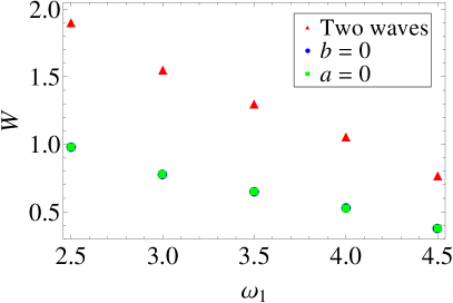
Figure 1: (Color online) The pair-production probability $W$ is calculated for selected values of the frequency $\omega_{1}$. We normalize the probability $W$ by $10^{-6}n_{\gamma}~{}{\rm{eV}}$, the average density $n_{\gamma}$ of the probe photon beam is in units of $({\rm eV})^{3}$, and the frequency $\omega_{1}$ is in units of eV. We show the results in the following cases: (i) a probe photon colliding with two plane waves; (ii) the probe photon colliding with each of these two plane waves. Here we choose the frequencies $\omega_{2}=100~{}\omega_{1}$ and the intensities of the fields $I_{1}=I_{2}=10^{18}~{}\rm{W/cm^{2}}$. For each value of $\omega_{1}$, the energy of the corresponding probe photon ($\sim 30$GeV) is selected (see Table 1) to make the probability of pair production off the probe photon colliding with one of the two plane waves and the probability of pair production off the probe photon colliding with the other plane wave to be almost the same (see the overlapping of full circles and squares).

III.2 Two and one plane-wave cases

In Fig. 1, we show the pair-production probability $W$ in the case of a probe photon colliding with two plane waves for different values of the frequency $\omega_{1}$ and the pair-production probability $W$ in the case of the probe photon colliding with each of these two plane waves. As shown in Fig. 1, the pair-production probability (we denote here as $W_{t}$) in the case of a probe photon colliding with two plane waves is larger than its corresponding probabilities ($W_{a}$ and $W_{b}$, $W_{a}\approx W_{b}$) in the case of the probe photon colliding with each of these two plane waves, but slightly smaller than the sum of these two probabilities ($W_{a}+W_{b}$), i.e.,

$$(W_{a}+W_{b})\gtrapprox W_{t}>W_{a,b}.$$ (24)

Here we introduce the notations $W_{a}=W|_{|b|=0}$ and $W_{b}=W|_{|a|=0}$ for the probability of pair creation off the probe photon colliding with each of these two plane waves, respectively, which are calculated by Eqs. (20)-(21). It is necessary to clarify here that the relation (24) is not true, in general, but only holds for the parameters of the laser waves and probe photon considered in this article; e.g., it does not hold for the case discussed in Ref. Jansen2013 . The result (24) can be understood from the point that the effective masses (9) of electrons and positrons in the two plane waves are slightly larger than the effective masses of electrons and positrons in one of these two plane waves. Therefore, in the case of two plane waves, the contribution to the pair-production probability from each plane wave is slightly suppressed by the slightly large effective mass. This leads to the result that $W_{t}\lessapprox(W_{a}+W_{b})$. We will give some further discussions below.

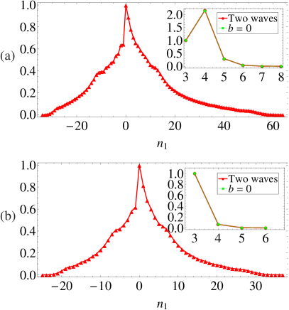
Figure 2: (Color online) The normalized pair-production probability $W_{1}(n_{1})$ is plotted as a function of $n_{1}$. The normalized pair-production probability $W_{ar}(n_{1})$ for the case of one plane wave ($|b|=0$) and $W_{0}(n_{1})$ are plotted in the inset. (a) $\omega_{1}=2.5~{}{\rm{eV}}$ and (b) $\omega_{1}=4~{}{\rm{eV}}$. Here we use the same parameters of the plane waves and probe photons as the ones used in Fig. 1.

III.3 The high multiphoton phenomenon and pair production with simultaneous photon emission

In order to the phenomenon of pair production with simultaneous photon emission into the low-frequency wave and high multiphoton phenomenon in this nonlinear Breit-Wheeler process (5), we study the pair-production probability for the process with the given $n_{1}$ and $n_{2}$ related to the given numbers ($|n_{1}|,|n_{2}|$) of photons absorbed from (emitted into) the two plane waves,

$$W_{t}(n_{1},n_{2})=\frac{e^{2}n_{\gamma}}{16\pi^{2}k^{\prime}_{0}}\int_{0}^{2\pi}d\phi\int_{1}^{u_{s}}\frac{du}{u\sqrt{u(u-1)}}\mathcal{M}(n_{1},n_{2}).$$ (25)

For the following discussions, we define the normalized pair-production probability for the process with the given $n_{1}$ and $n_{2}$ as

$$W_{n_{2}}(n_{1})=W_{t}(n_{1},n_{2})/W_{t}(n^{\rm thre}_{1}(n_{2}),n_{2}),$$ (26)

where $n^{\rm thre}_{1}(n_{2})$ is the minimum value of $|n_{1}|$ determined by Eq. (18) for a fixed value of $n_{2}$. For a comparison with the case of one plane wave ($|b|=0$), analogously to Eq. (26), we also define the normalized pair-production probability for the process with a given $n_{1}$ in the case when the high-frequency wave is absent ($|b|=0$) as

$$W_{ar}(n_{1})=W_{a}(n_{1})/W_{a}(n_{0}),$$ (27)

where $W_{a}(n_{1})$ is obtained from Eq. (20),

$$W_{a}(n_{1})=\frac{e^{2}n_{\gamma}}{16\pi^{2}k^{\prime}_{0}}\int_{0}^{2\pi}d\phi\int_{1}^{u_{s_{1}}}\frac{du}{u\sqrt{u(u-1)}}\mathcal{M}_{a}(n_{1}).$$ (28)

The results of $W_{0}(n_{1})$, $W_{1}(n_{1})$, and $W_{ar}(n_{1})$ for the cases of $\omega_{1}=2.5~{}{\rm{eV}}$ and $4~{}{\rm{eV}}$ are shown in Fig. 2. We show these results only for the two lowest numbers ($n_{2}=0,1$) of photons absorbed from the high-frequency wave field. The contributions from $n_{2}>1$ are very small because the $\xi_{2}$ under consideration is very small ($\xi_{2}\ll 1$). This is in agreement with the result of Refs. Ritus1985 ; Nikishov1964 . In addition, the contributions from negative values of $n_{2}$ are also very small. The reasons as follows. According to the threshold condition (18), when $n_{2}$ is negative, there must be a very large number of photons absorbed from the low-frequency wave ($n_{1}\gg 1$). However, the contributions from the processes with large $n_{1}$ ($n_{1}\gg 1$) are suppressed by the weak $\xi_{1}$ considered in this article.

It is shown in Fig. 2 that $W_{0}(n_{1})$ is rather close to $W_{ar}(n_{1})$ for each selected value of $\omega_{1}$. This can be understood as follows. In our calculations for $\xi_{1}\gg\xi_{2}$, the effects of the high-frequency wave on the wave function of electrons and positrons such as the spin correction, phase correction, and effective mass are small, compared to the effects of the low-frequency wave. In this regard, the influence of the high-frequency wave on the pair is very small for the process in which there is no photon absorbed from the high-frequency wave. More explicitly, this can be seen from the expression of $\mathcal{B}_{s}$ in Refs. Ritus1985 ; Nikishov1964 and the properties of the Bessel functions (see, e.g., Ref. Abramowitz1965 ) that $\mathcal{B}_{0}|_{n_{2}=0}\sim~{}1$, $\mathcal{B}_{1}|_{n_{2}=0}\sim~{}0$, and $\mathcal{B}_{2}|_{n_{2}=0}\sim~{}1/2$, for the parameters of the plane waves we use here. As a result, it is shown from Eqs. (25) and (28) that $W_{0}(n_{1})$ is close to $W_{ar}(n_{1})$.

In Fig. 2, $W_{ar}(n_{1})$ decreases rapidly as the value of $n_{1}$ increases. This result is in agreement with the discussion in Refs. Ritus1985 ; Nikishov1964 for the field strength parameter $\xi_{1}<1$. In this case, the main contributions to the probability of pair production off a probe photon colliding with one monochromatic plane wave are from the processes in which the number of photons absorbed from the wave is near the threshold value when the field strength parameter $\xi_{1}<1$. On the contrary, $W_{1}(n_{1})$ shows the high multiphoton phenomenon. As shown in Fig. 2, $W_{1}(n_{1})$ has a significant value even when the absorbed photon number $n_{1}$ is around $20$. The absorption of one photon from the high-frequency wave enhances the multiphoton processes of the low-frequency wave. It is also shown in Fig. 2 that when increasing the frequency $\omega_{1}$, the multiphoton phenomenon of $W_{1}(n_{1})$ is suppressed, consistent with the discussions Ritus1985 ; Nikishov1964 in which the multiphoton phenomenon dominantly depends on the field strength parameters $\xi_{1}$ and $\xi_{2}$. When the frequencies increase and the intensities do not change, $\xi_{1}$ and $\xi_{2}$ decrease, leading to a lower multiphoton phenomenon.

In Fig. 2, we show the phenomenon of Breit-Wheeler pair production with simultaneous photon emission (represented by the negative values of $n_{1}$) into the low-frequency wave by absorbing one photon from the high-frequency wave and the probe photon. In Fig. 2, the high multiphoton phenomenon is also shown in this Breit-Wheeler process with simultaneous photon emission into the low-frequency wave since $W_{1}(-|n_{1}|)$ has a significant value even when $|n_{1}|$ is large (e.g. $|n_{1}|\sim 20$). In addition, $W_{1}(-|n_{1}|)$ is smaller than $W_{1}(|n_{1}|)$ for a fixed $|n_{1}|$. This implies that, absorbing one photon from the high-frequency wave and the probe photon, the probability of Breit-Wheeler pair production with photon absorption from the low-frequency wave is larger than the probability of Breit-Wheeler pair production with simultaneous photon emission into the low-frequency wave. One of the reasons is that the former has a larger phase space of Breit-Wheeler pair production than the latter. We stress once again that this phenomenon of pair production with simultaneous photon emission into the wave cannot happen in the nonlinear Breit-Wheeler process of pair production off a probe photon colliding with one plane wave only (see the inset in Fig. 2).

In addition, we want to mention that, as shown in Fig. 2(a) for the case $\omega_{1}=2.5~{}{\rm{eV}}$, $W_{ar}(n_{1})$ first increases and then decreases, as $n_{1}$ increases. This is mainly because the selected value of $\zeta_{1}$ in this case leads to a threshold value $n_{0}$ very close to $3$. As a result, the phase space in the integration of Eq. (28) for the case $n_{1}=3$ is rather small compared to the one of the case $n_{1}=4$. This explains the results of $n_{1}=3$ and $n_{1}=4$ shown in Fig. 2(a).

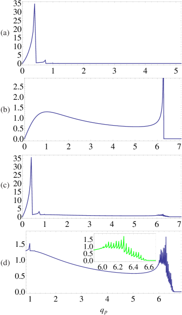
Figure 3: (Color online) The differential pair-production probability $dW/dq_{p}$ is normalized by $10^{-7}n_{\gamma}~{}{\rm{eV}}$. We plot it in terms of the transverse component $q_{p}$. Here we use the same parameters of the plane waves and probe photons adopted in Fig. 1 for $\omega_{1}=4~{}{\rm{eV}}$. (a): $dW/dq_{p}$ for the one-wave case of $|b|=0$. (b): $dW/dq_{p}$ for the one-wave case of $|a|=0$. (c) $dW/dq_{p}$ for the case of two waves. (d) Detailed results of $dW/dq_{p}$ for the case of two waves.

III.4 The pair spectrum

Now we turn to the spectra of the $e^{-}~{}e^{+}$ pair to give a further understanding and consequence of the phenomenon of pair production with simultaneous photon emission into the low-frequency wave and high multiphoton phenomenon shown in Fig. 2. From the four-quasimomentum conservation law (19) and the definition of the invariant variable $u$, we obtain the transverse component $|q_{\bot}|$ of $\vec{q}_{1}$ and $\vec{q}_{2}$, which are perpendicular to $\vec{k}$ ( $\vec{k}$ and $\vec{k^{\prime}}$ being oppositely directed),

$$|q_{\bot}|=m_{*}\sqrt{\frac{u_{s}}{u}-1}.$$ (29)

Introducing the dimensionless transverse momentum $q_{p}\equiv|q_{\bot}|/m$, from Eq. (15) we obtain the differential pair-production probability,

$$\frac{dW}{dq_{p}}=\sum_{n_{1},n_{2}}\frac{dW_{n_{1}n_{2}}}{dq_{p}},$$ (30)

and the differential pair-production probability of the process with the given $n_{1}$ and $n_{2}$,

$$\frac{dW_{n_{1}n_{2}}}{dq_{p}}=\frac{2uq_{p}}{(m_{*}/m)^{2}u_{s}\sqrt{u(u-1)}}\int_{0}^{2\pi}d\phi\mathcal{M}(n_{1},n_{2}).$$ (31)

From Eq. (20), we also obtain the differential pair-production probability for the case in which the high-frequency wave is absent ($|b|=0$),

$$\frac{dW}{dq_{p}}=\sum_{n_{1}}\frac{dW_{a}(n_{1})}{dq_{p}},$$ (32)

where the differential pair-production probability $dW_{a}(n_{1})/dq_{p}$ of a given $n_{1}$ can be obtained from Eq. (31) by $\mathcal{M}(n_{1},n_{2})\rightarrow\mathcal{M}_{a}(n_{1})$ and $u_{s}\rightarrow u_{s_{1}}$ of Eqs. (16) and (17). In the case when the low-frequency plane wave is absent ($|a|=0$), the differential pair-production probability $dW/dq_{p}$ can be obtained from Eqs. (21) and (32) by the substitutions $a\rightarrow b$, $k\rightarrow\kappa$, $n_{1}\rightarrow n_{2}$, and $\mathcal{A}_{s}\rightarrow\mathcal{B}_{s}$.

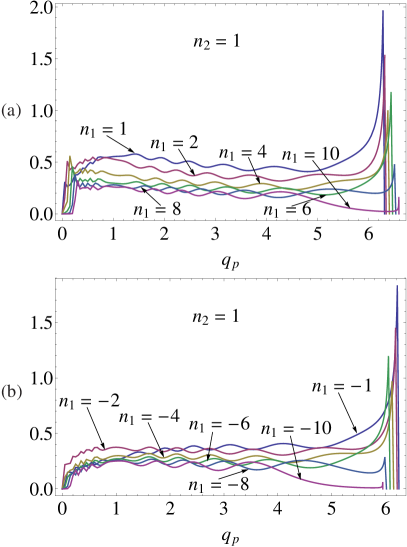
Figure 4: (Color online) The differential pair-production probability $dW_{n_{1}n_{2}}/dq_{p}$ for selected values of $n_{1}$ and $n_{2}$ is normalized by $10^{-8}n_{\gamma}~{}{\rm{eV}}$. We plot it in terms of $q_{p}$ for selecting values (a) $n_{1}=1,2,4,6,8,10$ with $n_{2}=1$ and (b) $n_{1}=-1,-2,-4,-6,-8,-10$ with $n_{2}=1$. Here we use the same parameters of the plane waves and probe photons adopted in Fig. 1 for $\omega_{1}=4~{}{\rm{eV}}$.

Figure 3 shows the differential pair-production probability $dW/dq_{p}$ for both one-wave and two-wave cases. Equation (29) indicates that the transverse component $q_{p}$ has a maximal value $q_{p}^{max}$ for the process with the given $n_{1}$ and $n_{2}$ related to the numbers ($|n_{1}|,|n_{2}|$) of photons absorbed from (emitted into) the waves,

$$q_{p}^{max}(n_{1},n_{2})=\frac{m_{*}}{m}\sqrt{u_{s}-1}$$ (33)

for the two-wave case and

$$q_{p}^{max}(n_{1})=\frac{m_{*}}{m}\sqrt{u_{s_{1}}-1}$$ (34)

for the case when the high-frequency wave is absent ($|b|=0$). The maximal value $q_{p}^{max}(n_{2})$ of transverse component $q_{p}$ for the case in which the low-frequency plane wave is absent ($|a|=0$) can be obtained from Eq. (34) by the substitutions $a\rightarrow b$, $k\rightarrow\kappa$, and $n_{1}\rightarrow n_{2}$. The existence of $q_{p}^{max}$ is due to the four-quasimomentum conservation (19). In Fig. 3, we show that, corresponding to the contributions from the processes with the different numbers of photons absorbed (emitted), the probability $dW/dq_{p}$ has different peaks located around $q_{p}\sim q_{p}^{max}$, and sharply decreases at $q_{p}^{max}$.

As shown in Fig. 3(a) for the presence of the low-frequency wave only, the differential pair-production probability practically vanishes after $n_{1}=4$, which corresponds to the maximal value $q_{p}^{max}(n_{1})|_{n_{1}=4}\approx 0.8$. Due to the fact that the field strength parameter $\xi_{2}\ll 1$, only the lowest order ($n_{2}=1$) term has a significant contribution to the pair-production probability for the case when the low-frequency wave field is absent ($|a|=0$), as we have discussed above in Fig. 2. The pair creation process in this case yields to the perturbation process considered by Breit and Wheeler Breit1934 . Its consequent result on the differential pair-production probability is clearly shown in Fig. 3(b): When $q_{p}$ is larger than the maximal value $q_{p}^{max}(n_{2})|_{n_{2}=1}\approx 6.25$ for $n_{2}=1$, the differential probability sharply decreases to zero.

Compared with the results presented in Figs. 3 (a) and 3(b) for the case of one wave, the multipeak structure of the differential pair-production probability $dW/dq_{p}$ presented in Figs. 3 (c) and 3(d) for the case of two waves clearly shows the phenomenon of pair production with simultaneous photon emission into the low-frequency wave and the high multiphoton phenomenon. As shown in the inset of Fig. 3 (d), the multipeaks of $dW/dq_{p}$ located at different values $q_{p}^{max}(n_{1},n_{2})$ indicate the multiphoton processes in which photons of different numbers ($|n_{1}|$) are absorbed from (emitted into) the low-frequency wave, in addition to the absorption of one photon $(n_{2}=1)$ from the high-frequency wave. In Fig. 4 (a), we plot $dW_{n_{1}n_{2}}/dq_{p}$, the detailed spectra of the created $e^{-}~{}e^{+}$ pair, absorbing $n_{1}$ photons from the low-frequency wave and one additional photon $(n_{2}=1)$ from the high-frequency wave. Due to the limit of the plotting scale, we only show the results of $n_{1}=1,2,4,6,8,10$ in Fig. 4(a). In Fig. 4 (b), we plot the detailed spectra $dW_{n_{1}n_{2}}/dq_{p}$ of the created $e^{-}~{}e^{+}$ pair by absorbing one photon $(n_{2}=1)$ from the high-frequency wave and emitting $|n_{1}|$ photons into the low-frequency wave.

We can learn from Fig. 4 how the multiphoton (absorption or emission) processes contribute to the total differential pair-production probability $dW/dq_{p}$ in Fig. 3. The multipeak structure of the total differential pair-production probability $dW/dq_{p}$ for $q_{p}>6.25$ presented in the inset of Fig. 3 (d) is due to the different peaks of the pair spectra after $q_{p}>6.25$ shown in Fig. 4 (a), which correspond to the contributions from the processes with the absorption of photons of different numbers ($n_{1}$) from the low-frequency wave, in addition to the absorption of one photon from the high-frequency wave. The multipeak structure of the total differential pair-production probability $dW/dq_{p}$ for $q_{p}<6.25$ presented in the inset of Fig. 3 (d) is due to the different peaks of the pair spectra after $q_{p}>5.8$ presented in Fig. 4 (b), which correspond to the contributions from the processes with the emission of photons of different numbers ($|n_{1}|$) into the low-frequency wave, in addition to the absorption of one photon from the high-frequency wave. In addition, the smooth oscillating structure of $dW_{n_{1}n_{2}}/dq_{p}$ for $q_{p}\lesssim 5.8$ in Fig. 4 indicates the interference effect of the two waves on the phase of the wave function of the pair (7). The results presented in Figs. 3 and 4 provide a possible way to access the phenomenon of pair production with simultaneous photon emission into the low-frequency wave and high multiphoton (absorption and emission) phenomenon in the nonlinear Breit-Wheeler process of pair production off a probe photon colliding with two plane waves (a low-frequency wave and a high-frequency wave), even for the case of the field strength parameter $\xi_{1,2}<1$.

In addition, we want to point out here that as shown in Figs. 3 and 4, the spectra $dW_{n_{1}n_{2}}/dq_{p}$ become large values around the maximal values $q_{p}^{max}(n_{1},n_{2})$ for fixed values of $(n_{1},n_{2})$. This is mainly due to the factor $1/\sqrt{u(u-1)}$ in the pair-production probability of Eqs. (15), (20) and (31). The integrations of Eqs. (15) and (20) over spectra $dW/dq_{p}$ are finite, i.e., the total pair-production probability $W$ is finite.

IV Summary and remarks

Based on the Volkov solutions of the Dirac equation in two plane waves, we studied the nonlinear Breit-Wheeler process of pair production off a probe photon colliding with a low-frequency and a high-frequency plane wave that propagate in the same direction. We analyzed the difference between the nonlinear Breit-Wheeler process (5) of $e^{-}~{}e^{+}$ pair production off a probe photon colliding with two plane waves and the process (1) of pair production off the probe photon colliding with each of these two plane waves.

The results show that the high multiphoton phenomenon is clearly evident in the nonlinear Breit-Wheeler process of pair production off a probe photon colliding with a low-frequency and a high-frequency plane wave. We also show the phenomenon of Breit-Wheeler pair production with simultaneous photon emission into the low-frequency wave by absorbing one photon from the high-frequency wave and the probe photon. This phenomenon of pair production with simultaneous photon emission into the wave cannot happen in the nonlinear Breit-Wheeler process of pair production off a probe photon colliding with one plane wave only. In the case of the electromagnetic plane waves of intensities $I_{1}=I_{2}=10^{18}~{}\rm{W/cm^{2}}$, the frequency $\omega_{1}\sim{\rm{eV}}$, and $\omega_{2}=100~{}\omega_{1}$, i.e., $\xi_{1}<1$ and $\xi_{2}\ll 1$, the contributions to the pair-production probability from the process with one photon ($n_{2}=1$) absorbed from the high-frequency wave and a large number ($|n_{1}|$) of photons absorbed from (or emitted into) the low-frequency wave are still significantly large even at $|n_{1}|\simeq 20$. As a comparison, in the absence of the high-frequency wave, the contributions to the pair-production probability from the processes can be negligible when the number of photons absorbed from the low-frequency wave is larger than $5$, i.e., $n_{1}>5$. This indicates that the multiphoton phenomenon cannot be evident in the presence of one plane wave only with field strength parameter $\xi_{1,2}<1$. This means that the presence of the high-frequency wave enhances the contributions of the low-frequency wave to the pair-production probability via the high multiphoton processes. We also present the spectra (multipeak structure) of the created $e^{-}~{}e^{+}$ pair to show the effects of the phenomenon of pair production with simultaneous photon emission into the low-frequency wave and high multiphoton (absorption and emission) phenomenon in this two-wave process. These phenomena can be studied by using the already available technology of lasers even for the wave field strength parameter $\xi_{1}<1$.

To end this article, we would like to mention that it would be interesting to make a systematic analysis of the nonlinear Breit-Wheeler processes of $e^{-}~{}e^{+}$ pair production off a probe photon colliding with two plane wave fields in the large range of parameters $\xi_{1}$, $\xi_{2}$, $\zeta_{1}$, and $\zeta_{2}$ of two plane waves and high-energy photons.

Acknowledgements

Authors are grateful to Prof.  Ruffini for his support and encouragement to work on the physics of strong fields. We are also grateful to the anonymous referee for his/her suggestions and comments, which helped us to improve our article. Yuan-Bin Wu is supported by the Erasmus Mundus Joint Doctorate Program through Grant Number 2011-1640 from the EACEA of the European Commission.

References

- (1) G. A. Mourou, T. Tajima, and S. V. Bulanov, Rev. Mod. Phys. 78, 309 (2006) and references therein.
- (2) A. Di Piazza, C. Müller, K. Z. Hatsagortsyan, and C. H. Keitel, Rev. Mod. Phys. 84, 1177 (2012) and references therein.
- (3) F. Sauter, Z. Phys. 69, 742 (1931).
- (4) W. Heisenberg and H. Euler, Z. Phys. 98, 714 (1936) [English translation: arXiv: physics/0605038].
- (5) J. Schwinger, Phys. Rev. 82, 664 (1951).
- (6) G. V. Dunne, in Ian Kogan Memorial Collection, From Fields to Strings: Circumnavigating Theoretical Physics (World Scientific, Singapore, 2005) and references therein.
- (7) R. Ruffini, G. Vereshchagin, and S.-S. Xue, Phys. Rep. 487, 1 (2010) and references therein.
- (8) http://www.xfel.eu.
- (9) http://laserstars.org/biglasers/pulsed/short/petawatt.html.
- (10) http://www.eli.laser.eu/.
- (11) D. L. Burke, R. C. Field, G. Horton-Smith et al., Phys. Rev. Lett. 79, 1626 (1997).
- (12) C. Bamber, S. J. Boege, T. Koffas et al., Phys. Rev. D 60, 092004 (1999).
- (13) Y. I. Salamin, S. X. Hu, K. Z. Hatsagortsyan, and C. H. Keitel Phys. Rep. 427, 41 (2006) and references therein.
- (14) G. V. Dunne, Eur. Phys. J. D 55, 327 (2009) and references therein.
- (15) H. Gies, Eur. Phys. J. D 55, 311 (2009) and references therein.
- (16) H. Kleinert and S.-S. Xue, Ann. Phys. 333, 104 (2013).
- (17) C. Kohlfürst, H. Gies, and R. Alkofer, Phys. Rev. Lett. 112, 050402 (2014).
- (18) G. Breit and J. A. Wheeler, Phys. Rev. 46, 1087 (1934).
- (19) H. R. Reiss, J. Math. Phys. 3, 59 (1962).
- (20) A. I. Nikishov and V. I. Ritus, Sov. Phys. JETP 19, 529 (1964).
- (21) A. I. Nikishov and V. I. Ritus, Sov. Phys. JETP 20, 757 (1965).
- (22) A. I. Nikishov and V. I. Ritus, Sov. Phys. JETP 25, 1135 (1967).
- (23) N. B. Narozhnyi, A. I. Nikishov, and V. I. Ritus, Sov. Phys. JETP 20, 622 (1965).
- (24) V. I. Ritus, J. Sov. Laser Res. 6, 497 (1985).
- (25) M. G. Hauser and E. Dwek, Annu. Rev. Astron. Astr. 39, 249 (2001).
- (26) F. A. Aharonian, Very High Energy Cosmic Gamma Radiation (World Scientific, Singapore, 2003).
- (27) T. Heinzl, A. Ilderton, and M. Marklund, Phys. Lett. B 692, 250 (2010).
- (28) A. I. Titov, H. Takabe, B. Kämpfer, and A. Hosaka, Phys. Rev. Lett. 108, 240406 (2012).
- (29) T. Nousch, D. Seipt, B. Kämpfer, and A. I. Titov, Phys. Lett. B 715, 246 (2012).
- (30) K. Krajewska and J. Z. Kamiński, Phys. Rev. A 86, 052104 (2012).
- (31) A. I. Titov, B. Kämpfer, H. Takabe, and A. Hosaka, Phys. Rev. A 87, 042106 (2013).
- (32) R. Schützhold, H. Gies, and G. Dunne, Phys. Rev. Lett. 101, 130404 (2008).
- (33) S. S. Bulanov, V. D. Mur, N. B. Narozhny, J. Nees, and V. S. Popov, Phys. Rev. Lett. 104, 220404 (2010).
- (34) G. V. Dunne, H. Gies, and R. Schützhold, Phys. Rev. D 80, 111301(R) (2009).
- (35) A. Di Piazza, E. Lötstedt, A. I. Milstein, and C. H. Keitel, Phys. Rev. Lett. 103, 170403 (2009).
- (36) V. A. Lyul’ka, Sov. Phys. JETP 40, 815 (1975).
- (37) V. A. Lyul’ka, Sov. Phys. JETP 45, 452 (1977).
- (38) V. A. Lyul’ka, Sov. Phys. JETP 42, 408 (1975).
- (39) D. M. Volkov, Z. Phys. 94, 250 (1935).
- (40) V. B. Berestetskii, E. M. Lifshitz, and V. B. Pitaevskii, Quantum Electrodynamics (Pergamon Press, New York, 1982).
- (41) M. Pardy, Int. J. Theor. Phys. 45, 647 (2006).
- (42) N. B. Narozhny and M. S. Fofanov, JETP 90, 415 (2000).
- (43) M. J. A. Jansen and C. Müller, Phys. Rev. A 88, 052125 (2013).
- (44) M. Abramowitz and I. A. Stegun, Handbook of Mathematical Functions (Dover, New York, 1965).