A Hierarchical Graphical Model for Big Inverse Covariance Estimation with an Application to fMRI

Xi Luo

Brown University

Abstract. Brain networks has attracted the interests of many neuroscientists. From functional MRI (fMRI) data, statistical tools have been developed to recover brain networks. However, the dimensionality of whole-brain fMRI, usually in hundreds of thousands, challenges the applicability of these methods. We develop a hierarchical graphical model (HGM) to remediate this difficulty. This model introduces a hidden layer of networks based on sparse Gaussian graphical models, and the observed data are sampled from individual network nodes. In fMRI, the network layer models the underlying signals of different brain functional units, and how these units directly interact with each other. The introduction of this hierarchical structure not only provides a formal and interpretable approach, but also enables efficient computation for inferring big networks with hundreds of thousands of nodes. Based on the conditional convexity of our formulation, we develop an alternating update algorithm to compute the HGM model parameters simultaneously. The effectiveness of this approach is demonstrated on simulated data and a real dataset from a stop/go fMRI experiment.

Keywords: Convex optimization; Graphical models; functional MRI; K-means; Lasso.

1 Introduction

Graphical models is a statistical tool to describe the relationships between multiple variables. In functional MRI or fMRI, the variables are the Blood-Oxygen-Level-Dependent (BOLD) activities at different regions (also known as voxels) of the human brain. One important scientific question is how these brain regions are connected, which is termed brain connectivity. However, the dimensionality of whole-brain fMRI data is usually in hundreds of thousands, and this scale challenges direct application of existing methods. Recently, large-scale brain network estimation is regarded as a “big data” problem (Turk-Browne, 2013), and has raised several challenges and opportunities (Sporns, 2014). In this paper, we propose a novel approach to provide interpretable and direct estimation from whole-brain fMRI data, and this general approach may have applications for other big data problems as well.

The fMRI dataset in this paper comes from one subject performing a cognitive experiment–stop/go trials, which is made publicly available by its investigators (Xue et al., 2008). After preprocessing the data (see details in Section 4), it consists of the BOLD measures from $230,590$ voxels in $180$ time points. Due to the dimensionality, previous research on stop/go fMRI has been focusing on individual voxel activations, and their implications for phenotypes and behavior outcomes. For instance, stop/go voxel activations have been studied using meta-analysis (Simmonds et al., 2008) and causal inference (Luo et al., 2012), and the activity predicts substance use and behavior (Chiang-shan et al., 2010; Luo et al., 2013). The problem of studying the whole brain connections is an emerging and important direction, but is also challenging methodologically.

There are two major types of connectivity analysis: functional connectivity and effective connectivity, see Friston (2011), Smith et al. (2013), and Bowman (2014) for review. The simplest measure for inferring functional connectivity is probably pair-wise correlations. This is computationally inexpensive but is less biologically meaningful (Buckner, 2010; Smith et al., 2013). For example, it does not differentiate direct and indirect connections. Alternative approaches include clustering (Goutte et al., 1999; Bowman and Patel, 2004), and independent component analysis or ICA (Calhoun et al., 2001; Beckmann and Smith, 2004; Guo, 2011; Eloyan et al., 2013). However, they again lack identification of direct and indirect connections. Effective connectivity, on the other hand, seeks to infer directional relationships between directly connected brain regions. The popular approaches for effective connectivity include dynamic causal modeling (Friston et al., 2003), structural equation models, and Granger causality. Because these tools are complex in computation and modeling, they are usually applied for a small number (e.g. $<100$) of preselected voxels or regions. The selection criteria include prior knowledge (e.g. anatomical and functioning annotations), and functional activation (Duann et al., 2009). Recently, voxel correlations are used provide more accurate selection of voxels for a certain region of the brain (Zhang and Li, 2014). Despite these attempts, the result, however, may be sensitive to the selection of regions (Bowman, 2014), and the network inference can be biased if the influence from other omitted regions is large. Several challenges remain in inferring large-scale direct connectivity (Varoquaux and Craddock, 2013; Sporns, 2014).

To infer large-scale connectivity, we will further develop a popular type of graphical models, called sparse Gaussian graphical models (Yuan and Lin, 2007; Banerjee et al., 2008), hereafter sGGM. This type of models has a solid probabilistic foundation for differentiating direct and indirect connections (Dempster, 1972; Lauritzen, 1996). Suppose we observe a multivariate observation $\mathbf{X}_{n\times p}$ , with $n$ iid observations from a $p$-variate normal distribution $N\left(\mathbf{\mu},\mathbf{\Sigma}\right)$. sGGM represents the relationships between $p$ variables by a network of $p$ nodes, where each node represents a variable and there are parsimonious connections between nodes. Methodologically, inference of the connections between $p$ nodes is reduced to estimate a sparse inverse covariance $\mathbf{\Omega}=\mathbf{\Sigma}^{-1}$, where a nonzero off-diagonal entry in $\mathbf{\Omega}$ means that the corresponding row and column variables/nodes are directly connected and a zero entry means no connections, see Lauritzen (1996). In fMRI applications, direct connectivity is more biologically interpretable than indirect functional connectivity (Friston, 2011). The sGGM approach also performs reasonably well on a simulation study using a small number of regions (Smith et al., 2011).

Recently, several estimators for sGGM have been proposed based on the $\ell_{1}$ heuristic (Chen and Donoho, 1994; Tibshirani, 1996). These approaches can be roughly divided according three major estimation principals: penalized conditional likelihood or neighborhood selection (Meinshausen and Bühlmann, 2006; Yuan, 2010), penalized full likelihood or Graphical lasso (Yuan and Lin, 2007; Banerjee et al., 2008; Friedman et al., 2008), and algebraic properties (Cai et al., 2011; Liu and Luo, 2012). The last type, especially, has faster statistical convergence rates for a general class of distributions with polynomial tails (Cai et al., 2011), and is statistically adaptive and computationally efficient (Liu and Luo, 2012). However, all these approaches don’t scale up to hundreds of thousands of nodes, though a large scale algorithm for penalized likelihood is proposed recently by Hsieh et al. (2013).

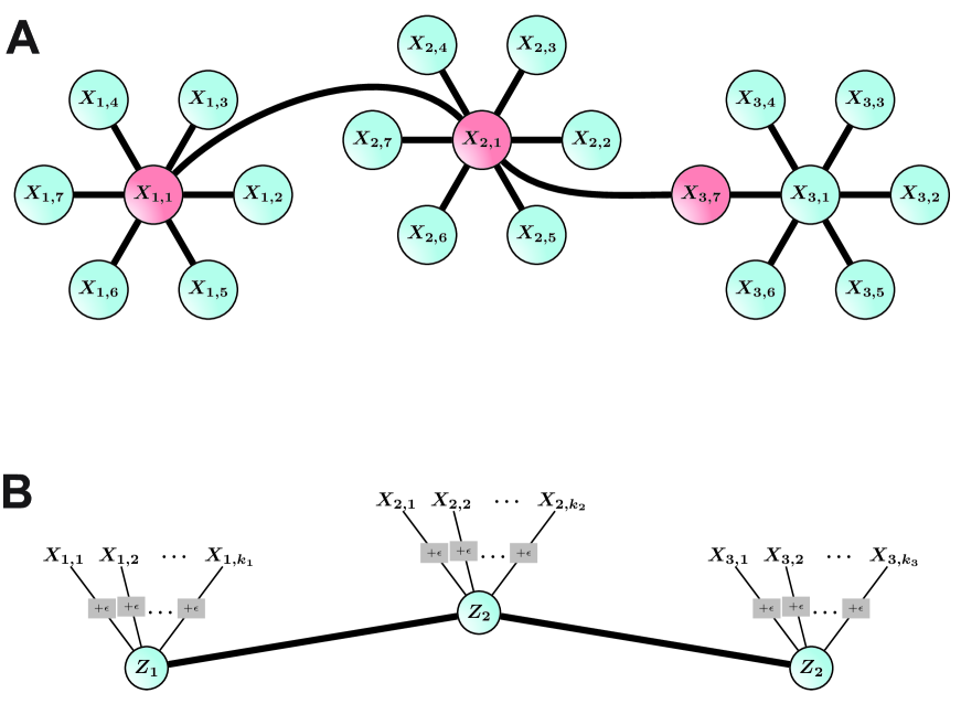
The brain network system is rather complex, compared to the standard sGGM model. For instance, the brain network has a hierarchical structure: billions of connected neurons excite BOLD measures in hundreds of thousands of voxels, connected voxels form areas (e.g. motor area), connected areas form systems (e.g. motor system), and systems interact with each other. Graph theoretical analysis yields insight understanding of the network complexity, see Bullmore and Sporns (2009) for review. A popular network structure is shown in Figure 1A, in which communities of nodes are connected with each other via hub nodes (Power et al., 2013). This network structure has also been proposed for other biological networks, for example genetic networks (Guimera and Amaral, 2005). It was unclear how these structures were represented in large-scale network estimation methods, including sGGM.

Leveraging these scientific findings and methodological advances, we propose a simple and unified statistical model for big network data generated in a particular way. A conceptual sketch of this model is plotted in Figure 1B. We employ a hidden layer of variables to model the network, and the observations are multiple noisy samples from each node. This model shares similar topological structures with the hub network (Figure 1A), but incorporate the special characteristics (e.g. smoothness) of fMRI, see Section 2. Under this framework, we describe three goals: signal extraction, voxel clustering, and network estimation. These three goals are interwoven with each other. We thus develop a generic alternating updating algorithm for carrying out them simultaneous, see Section 3. The advantages of our method are demonstrated on the fMRI data in Section 4 and on simulated data in Section 5. We will conclude with discussion in Section 6. The technical details are postponed to Section 7.

Figure 1: Schematic plots of (A) a biological network model with hubs and communities (Guimera and Amaral, 2005; Power et al., 2013) and (B) the HGM model. The biological network model assumes that data are sampled from all nodes $X_{i,j}$, including the hub nodes $X_{1,0}$, $X_{2,0}$, and $X_{3,7}$, shown in red. The HGM model assumes a hidden network of 3 nodes $Z_{i}$, $i=1,2,3$. The observed data $X_{i,j}$, $j=1,\dotsc,k_{i}$, are the corresponding $Z_{i}$ plus independent noises. Network nodes are shown in circles, and all the subscript indexes are arbitrary.

2 A Hierarchical Graphical Model

We first collect the notations used in this paper. Let $\mathbf{M}=(M_{ij})$ be any matrix. $M_{\cdot j}$ stands for the $j$th column of $\mathbf{M}$, and $M_{i\cdot}$ for the $i$th row. The following matrix norms on $\mathbf{M}$ will be used: $\left\|\mathbf{M}\right\|_{2}=\sqrt{\sum_{i}\sum_{j}M_{ij}^{2}}$ for the Frobenius norm; $\left\|\mathbf{M}\right\|_{1}=\sum_{i,j}\left|M_{ij}\right|$ for the $\ell_{1}$ norm. The trace and determinant of $\mathbf{M}$ are denoted by $\operatorname{tr}\left(\mathbf{M}\right)$ and $\det\left(\mathbf{M}\right)$ respectively. A diagonal matrix is denoted by $\operatorname{diag}\left(M_{1},\dotsc,M_{p}\right)$ where the diagonal entries $M_{i}$ are shortened notations for $M_{ii}$ for any $i$. The cardinality of a set $S$ is given by $\left|S\right|$.

We now introduce the formulation of our hierarchical graphical model. Without loss of generality, we assume all variables in our model are mean centered. This could be achieved by subtracting the mean for each variable first. In fMRI, the means are usually arbitrary, and a mean centering approach is usually employed in the preprocessing pipeline.

Suppose that all the $p$ variables/columns of the observed data matrix $\mathbf{X}$ are separated into one and only one of the $K$ disjoint group sets $G_{k}\subset\left\{1,\dotsc,p\right\}$, $k=1,\dotsc,K$. We introduce a hierarchical variable denoted by $\mathbf{Z}$, where each column $Z_{\cdot k}$ represents the hidden signal for group $G_{k}$. The hierarchical variable $\mathbf{Z}$ relates to the observed variable $\mathbf{X}$ as

$$X_{ij}=Z_{ik}+\epsilon_{ijk}\qquad\mbox{for}\,j\in G_{k},\,i=1,\dotsc,n,\,k=1,\dotsc,K,$$ (1)

where the noise variables $\epsilon_{ijk}\sim N\left(0,\phi_{k}\right)$ for group $k$ are independent of each other and independent of all $\mathbf{Z}$ . Denote the error variance matrix $\mathbf{\Phi}=\operatorname{diag}\left(\phi_{1},\dotsc,\phi_{K}\right)$. As discussed in the introduction, we assume each row of the hierarchical variable is

$$Z_{i\cdot}\overset{iid}{\sim}N\left(\mathbf{0},\mathbf{\Sigma}\right)$$ (2)

where the inverse covariance (or precision) matrix is $\mathbf{\Omega}=\mathbf{\Sigma}^{-1}$.

The observed $\mathbf{X}$ under Model (1) and (2) is still multivariate normal, and thus can be represented by a Gaussian graphical model. It is possible to directly estimate a $p\times p$ precision matrix $\mathbf{\Omega}_{X}$ of $\mathbf{X}$ for moderate size $p$, using existing algorithms (Friedman et al., 2008; Cai et al., 2011; Liu and Luo, 2012). This task, however, becomes very challenging in computation and storage at least, when $p$ is in the size of hundreds of thousands. We will instead estimate a smaller precision matrix $\mathbf{\Omega}$ of size $K\times K$ based on the hierarchical variable $\mathbf{Z}$, where $K$ could be much smaller than $p$. The introduction of the hierarchical variable $\mathbf{Z}$ and the group assignment $G$ provides additional advantages in modeling and interpretation as we will outline below.

The group assignment $G$ makes the resulting network model interpretable because each node can be interpreted as a functional unit that consists of several variables. In fMRI, $\mathbf{X}$ is the original data where each column is a voxel, and the voxels in each $G_{k}$ forms a unit commonly known as area or region of interest (ROI) to neuroscientists. Our approach allows $G$ to be fixed based on prior knowledge or estimated from the data by an iterative algorithm in Section 3.

The hierarchical variable $\mathbf{Z}$ models the underlying signal within each group $G_{k}$, and we also use it to model the topological role of hubs. Given the group assignment $G$, an popular estimate for $\mathbf{Z}$ is given by, for each observation $i$,

$$\bar{Z}_{ik}=\frac{1}{\left|G_{k}\right|}\sum_{j\in G_{k}}X_{ij},\quad\mbox{for}\,k=1,\dotsc,K.$$

This is a common method for extracting signals from ROIs in fMRI analysis. As we will show momentarily, our estimator of $\mathbf{Z}$ is different from $\bar{\mathbf{Z}}$ by incorporating other model parameters, such as the network $\mathbf{\Omega}$.

3 Method

3.1 Likelihood Formulation and Convexity

We introduce the approach to estimate the parameters $\left(\mathbf{Z},G,\mathbf{\Omega},\mathbf{\Phi}\right)$ in Model (1) and (2). We consider two sGGM algorithms, Glasso (Friedman et al., 2008) or SCIO (Liu and Luo, 2012). Because both are motivated by the penalized likelihood framework, we will focus on describing the likelihood approach first, while the difference will emerge later. The negative log-likelihood function under our hierarchical model is, ignoring constants and scaling factors,

$$L\left(\mathbf{Z},G,\mathbf{\Omega},\mathbf{\Phi}\right)=\sum_{k=1}^{K}\left[\sum_{j\in G_{k}}\left\|X_{\cdot j}-Z_{\cdot k}\right\|_{2}^{2}/\left(n\phi_{k}\right)+\left|G_{k}\right|\log\phi_{k}\right]\\ +\frac{1}{n}\operatorname{tr}\left(\mathbf{Z}\mathbf{\Omega}\mathbf{Z}^{T}\right)-\log\det\left(\mathbf{\Omega}\right)+K\log\left(2\pi\right).$$ (3)

To introduce sparsity on $\Omega$, we consider a LASSO penalty (i.e. the $\ell_{1}$ norm) formulation via minimizing the following objective

$$L\left(\mathbf{Z},G,\mathbf{\Omega},\mathbf{\Phi}\right)+\lambda\left\|\mathbf{\Omega}\right\|_{1}$$ (4)

where $\lambda>0$ is a penalization parameter. The objective function (4) is unfortunately not jointly convex in $\left(\mathbf{Z},G,\mathbf{\Omega},\mathbf{\Phi}\right)$. The group assignment $G$ is a combinatorial optimization problem in general, which is NP-hard. However, the objective is conditionally convex in all the other parameters, summarized in the following proposition.

Proposition 1.

The objective function (4) is conditionally convex in $\mathbf{Z}$, $\mathbf{\Omega}$ and $\mathbf{\Phi}^{-1}$ respectively, conditional on all the other parameters in $\left(\mathbf{Z},G,\mathbf{\Omega},\mathbf{\Phi}\right)$.

3.2 An Alternating Update Algorithm

Due to the conditional convexity in Proposition 1, we propose to solve the problem via alternating iterative updates of each parameter, where the updating step minimizes the conditional objective function. Though the conditional minimization problem is not convex in the group assignment $G$, similar alternating procedures have been effective in practice (Lloyd, 1982; Forgy, 1965; MacQueen et al., 1967; Hartigan and Wong, 1979). Our algorithm also incorporates a group update step.

The conditional minimization for $\mathbf{Z}$ and $\mathbf{\Phi}^{-1}$ are given in explicit forms in the following proposition. Though the minimization is over $\mathbf{\Phi}^{-1}$, the solution is conveniently given in terms of $\mathbf{\Phi}$. The conditional minimization over $\mathbf{\Omega}$ is equivalent to the Glasso problem.

Proposition 2.

The conditional minimizer for $\mathbf{Z}$ in (4) is

$$\mathbf{Z}^{*}=\bar{\mathbf{Z}}\mathbf{D}_{G}\left[\mathbf{D}_{G}+\mathbf{\Omega}\mathbf{\Phi}\right]^{-1}$$

where $\mathbf{D}_{G}=\operatorname{diag}\left(\left|G_{1}\right|,\dotsc,\left|G_{K}\right|\right)$. That is, $\mathbf{Z}^{*}$ minimizes the following conditional minimization objective, while $\left(G,\mathbf{\Omega},\mathbf{\Phi}\right)$ are fixed,

$$L_{\mathbf{Z}}=\sum_{k=1}^{K}\sum_{j\in G_{k}}\left\|X_{\cdot j}-Z_{\cdot k}\right\|_{2}^{2}/\left(n\phi_{k}\right)+\frac{1}{n}\operatorname{tr}\left(\mathbf{Z}\mathbf{\Omega}\mathbf{Z}^{T}\right).$$

The conditional minimizer for $\mathbf{\Phi}$ is

$$\phi_{k}^{*}=\frac{1}{n\left|G_{k}\right|}\sum_{j\in G_{k}}\left\|Z_{\cdot k}-X_{\cdot j}\right\|_{2}^{2},\quad\mbox{for}\,k=1,\dotsc,K,$$

where the conditional objective is

$$L_{\mathbf{\Phi}^{-1}}=\frac{1}{n}\sum_{k=1}^{K}\left[\phi_{k}^{-1}\sum_{j\in G_{k}}\left\|X_{\cdot j}-Z_{\cdot k}\right\|_{2}^{2}-\left|G_{k}\right|\log\phi_{k}^{-1}\right].$$

The conditional minimization problem of $\mathbf{\Omega}$ is equivalent to the Glasso objective

$$L_{\mathbf{\Omega}}=\frac{1}{n}\operatorname{tr}\left(\mathbf{Z}\mathbf{\Omega}\mathbf{Z}^{T}\right)-\log\det\left(\mathbf{\Omega}\right)+\lambda\left\|\mathbf{\Omega}\right\|_{1}.$$

We use the conditional minimizers for $\mathbf{Z}$ and $\mathbf{\Phi}$ as our iterative updates respectively. Because the purpose of minimizing $L_{\mathbf{\Omega}}$ is to produce a sparse precision matrix $\mathbf{\Omega}$, we consider two approaches, Glasso and SCIO. Glasso minimizes $L_{\mathbf{\Omega}}$ exactly, and SCIO is based on the algebraic properties derived from $L_{\mathbf{\Omega}}$ (Cai et al., 2011; Liu and Luo, 2012), which has faster convergence rates for $\mathbf{\Omega}$ under moderate distribution assumptions (e.g. heavier tails). Because SCIO does not enforce positive definiteness of the precision matrix, we perform a simple refitting approach to ensure such (Cai et al., 2011).

The update rule for $\mathbf{Z}$ is a linear combination of $\bar{\mathbf{Z}}$, where the combination depends on other parameters. Due to the shrinkage effect by the hierarchical variable (Lehmann and Casella, 1998), our estimate is expected to have smaller MSEs than $\bar{\mathbf{Z}}$.

The algorithm for solving our hierarchical graphical model problem is summarized in Algorithm 1. The convergence criterion for stopping the iterative updates is

$$\frac{\left\|\mathbf{Z}^{\left(t-1\right)}-\mathbf{Z}^{\left(t\right)}\right\|_{2}}{\max\left(1,\left\|\mathbf{Z}^{\left(t-1\right)}\right\|_{2}\right)}<e_{\mbox{tol}}\quad\mbox{and}\quad G^{\left(t\right)}=G^{\left(t-1\right)}$$ (5)

where $e_{\mbox{tol}}$ is a tolerance level (e.g. $10^{-4}$), $\mathbf{Z}^{\left(t\right)}$ is the update at iteration $t$, and similar definition for $G^{\left(t\right)}$, $\mathbf{\Omega}^{\left(t\right)}$, and $\mathbf{\Phi}^{\left(t\right)}$.

There are many ways to update $G$ in step 4 of Algorithm 1. For simplicity, we use a hybrid rule for finding the group assignment $G$. In the initialization stage, we set $\left(\mathbf{Z}^{\left(0\right)},G^{\left(0\right)}\right)$ from Hartigan’s k-means (Hartigan and Wong, 1979) because it usually provides good clustering in practice. We then use $\left(\mathbf{Z}^{\left(0\right)},G^{\left(0\right)}\right)$ in step 2 and 3 to initialize $\mathbf{\Omega}^{\left(0\right)}$ and $\mathbf{\Phi}^{\left(0\right)}$. For the sequential alternating updates, we use a simple assignment rule suggested by Lloyd (1982), Forgy (1965), and MacQueen et al. (1967), where each point is reassigned to the closest cluster center $Z_{\cdot k}$. Because k-means suffers from the issue of converging to a local optima, our alternating algorithm may also suffer from this issue. Thus, we consider multiple runs of our algorithm and select the one with the largest likelihood.

Initialize: $\left(\mathbf{Z}^{\left(0\right)},G^{\left(0\right)},\mathbf{\Omega}^{\left(0\right)},\mathbf{\Phi}^{\left(0\right)}\right)$, $t=0$.

Repeat until the convergence criterion (5) is met:

1. Given $\left(\mathbf{Z}^{\left(t\right)},G^{\left(t\right)},\mathbf{\Omega}^{\left(t\right)},\mathbf{\Phi}^{\left(t\right)}\right)$, update $\mathbf{Z}^{\left(t+1\right)}=\bar{\mathbf{Z}}\mathbf{D}_{G^{\left(t\right)}}\left[\mathbf{D}_{G^{\left(t\right)}}+\mathbf{\Omega}^{\left(t\right)}\mathbf{\Phi}^{\left(t\right)}\right]^{-1}$.

2. Given $\left(\mathbf{Z}^{\left(t+1\right)},G^{\left(t\right)},\mathbf{\Omega}^{\left(t\right)},\mathbf{\Phi}^{\left(t\right)}\right)$, update $\phi_{k}=\frac{1}{n\left|G_{k}\right|}\sum_{j\in G_{k}}\left\|Z_{\cdot k}-X_{\cdot j}\right\|_{2}^{2}$ for $k=1,\dotsc,K$.

3. Given $\left(\mathbf{Z}^{\left(t+1\right)},G^{\left(t\right)},\mathbf{\Omega}^{\left(t\right)},\mathbf{\Phi}^{\left(t+1\right)}\right)$, update $\mathbf{\Omega}^{\left(t+1\right)}$ by a precision matrix estimation method (either Glasso or SCIO).

4. Given $\left(\mathbf{Z}^{\left(t+1\right)},G^{\left(t\right)},\mathbf{\Omega}^{\left(t+1\right)},\mathbf{\Phi}^{\left(t+1\right)}\right)$, update $G^{\left(t+1\right)}$ such that each $X_{\cdot j}$ is re-assigned to the closest center $Z_{\cdot k}$.

5. Update $t=t+1$.

Algorithm 1 An alternating update algorithm for estimating the HGM parameters.

3.3 Choice of the Tuning Parameters

Our model contains two tuning parameters, $K$ and $\lambda$. These can be chosen using either existing scientific knowledge or model selection methods. We employ the scientific choice in Section 4, and here we describe a model selection approach when such scientific knowledge is not available. The Bayesian Information Criterion (BIC) for our model is

$$L_{K,\lambda}+\frac{\log p}{n}\left(s/2+p+K\left(n+2\right)-1\right)$$

where $L_{K,\lambda}$ is the negative log-likelihood (3) with the choice of $K$ and $\lambda$, evaluated at the converged solution produced by Algorithm 1, and $s$ is the number of nonzeros in the off-diagonals of the solution $\mathbf{\Omega}$. The model complexity component in above consists of those of k-means (Pelleg et al., 2000) and sGGM. That is, there are $K-1$ class probabilities from $G$, $K$ variance estimates from $\mathbf{\Phi}$, $Kn$ estimates from $\mathbf{Z}$, $s/2+p$ nonzeros from $\mathbf{\Omega}$. The tuning parameter $\lambda$ controls the number of nonzeros in $\mathbf{\Omega}$, and one can perform a grid search on $\lambda$ first to pick the value yielding the smallest BIC. The tuning parameter $K$ controls the number of groups. One then compares the minimal BIC values from the previous step with different choices of $K$, and chooses the $K$ that produces the smallest BIC.

4 A fMRI Study on Motor Prohibition

We use an fMRI dataset (Xue et al., 2008) to illustrate the effectiveness of HGM. The dataset is publicly available from Open fMRI (https://openfmri.org/data-sets) under the accession number ds000007. This whole dataset consists of 20 subjects scanned under several sessions, with different kinds of stop/go event tasks. For the illustration purpose, we analyze the session 1 data of subject 1.

As suggested by the authors (Xue et al., 2008), we employ the same preprocessing pipeline implemented in the FMRIB software library (FSL, available from http://fsl.fmrib.ox.ac.uk/fsl/fslwiki/). Briefly, the pipeline includes slice timing correction, alignment, registration, normalization to the average 152 T1 MNI template, and smoothed with a 5mm full-width-half-maximum Gaussian kernel. The data are denoised using the FSL MELODIC procedure and a high pass filter with a 66s cut-off. After preprocessing, general linear models (GLM) for each voxel (Friston et al., 1994) are used to remove the non-stationary components, including motion and event related activation. The standardized GLM residuals are retained for our HGM analysis. The residuals are assumed to be stationary, similar to resting-state fMRI (Fair et al., 2007).

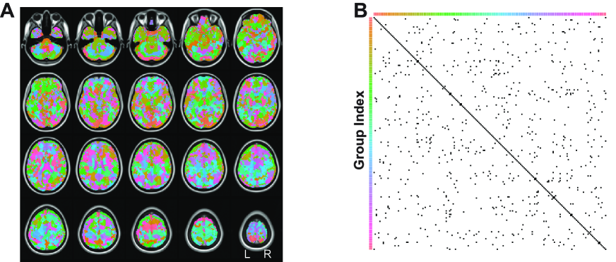
The processed dataset consists of the residual BOLD activity from 230,590 voxels in 180 time points, or equivalently an input matrix $X$ with $n=180$ and $p=230,590$. To make each variable in $X$ comparable, we standardize each one to have mean zero and unit variance. To illustrate the complex networks that can be recovered by HGM, we fix $K=200$ and $\lambda=0.5$, because these choices roughly matches the usual number of brain parcellations, for example the AAL atlas (Tzourio-Mazoyer et al., 2002). The resulting network has interesting scientific interpretations as well. Other choices can be taken depending on the scientific goals. For example, larger $K$ will give finer parcellations of the brain, smaller $\lambda$ usually yields densely connected networks, and vice versa.

We will use the SCIO update in Algorithm 1, because it shows higher accuracy for recovering the network edges in our simulation study (Section 5). To avoid local minima, due to group assignments, our HGM algorithm (Algorithm 1) is repeated 10 times with random starts. More number of repeats are allowed if more computing resources are available, but we find that 10 repeats are sufficient and the parcellations are stable, see Section 5 for a simulation evaluation as well. The repeat with the largest likelihood is reported in Figure 2. To a certain extent, the voxel grouping shows symmetry between left and right hemispheres, though this is not imposed in HGM. This approximate bilateral symmetry coincides with the classic theory of (approximately) mirrored functions of the two hemispheres. We thus are inclined to postulate that the HGM grouping recovers different functional units. It is challenging to visualize all the resulting voxel groups and their connections in Figure (2)B, and we thus examine one group and its connections in detail.

Figure 2: Recovered voxel groups (A) and network edges (B) by HGM. (A) voxel groups are indexed by color, overlaid on the average 152 T1 MNI template. (B) Connections between two groups are shown in black entries in the matrix, where the two groups are given by the row and column index colors respectively; no connections are shown in white. L: left; R: right.

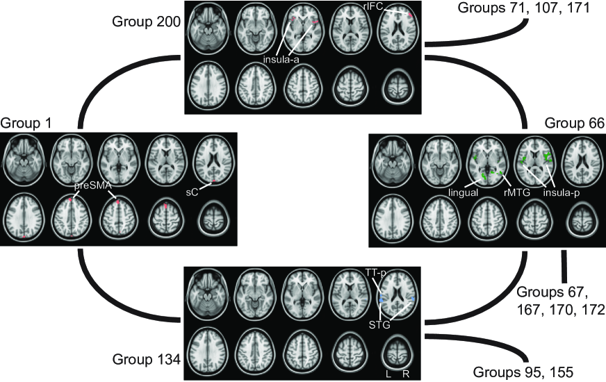
The region preSMA (anterior part of supplementary motor area) has been shown to play an important role during stop/go trails (Duann et al., 2009), and it is tagged as group 1 by HGM. Note that the group index numbers are arbitrary. We examine the overlays of big voxel clusters ($\geq 100$ voxels) in group 1 and three other directly or indirectly connected groups, see Figure 3. The detailed coordinates and cluster sizes are included in the supplemental material of this paper. Each group may contain multiple regions clustered together, and most of them are closely located in the brain and mirrored on both left and right hemispheres. The specific clusters in HGM also provides new insight about the wiring around preSMA, partly because HGM performs simultaneously brain parcellation and direct connectivity estimation. For instance, the connection between preSMA and rIFC (right inferior frontal cortex) have been studied before using a small Granger model (Duann et al., 2009), and here the whole brain HGM suggests that this connection is direct even if considering the whole brain activity. Moreover, insula activation has been implicated in a previous stop/go study (Luo et al., 2013), and it also correlates with preSMA (Zhang et al., 2012). HGM provides a more detailed map of anterior insula and rIFC (in group 200), which is directly connected to the preSMA group (group 1). This connection is termed the salience network (Seeley et al., 2007). The inclusion of rIFC and the exclusion of other salience network regions prompt an interesting question how the connections within this network are wired, for example whether the insula correlation is a consequence or cause of the direct connectivity between rIFC and preSMA. Furthermore, our HGM result also suggests that the insula grouping depends on the anterior (group 200) and posterior (group 65) positions, consistent with the findings from several studies (Anderson et al., 2011; Jakab et al., 2012; Kelly et al., 2012). Finally, the preSMA group contains two distant regions, preSMA and superior part of cuneus (or Brodmann area 19, superior), which is probably due to the role of the latter in motion-related visual processes. These two regions are also clustered by an ICA study (Sauvage et al., 2011). These coherent results suggest that further investigation is needed to study the possible connection between these two regions.

Figure 3: The overlays of voxel groups on the average 152 T1 MNI template, for the preSMA group (group 1) recovered by HGM, two directly connected groups (134, 200), and one group (group 66) connected to the previous two groups. The group index numbers are arbitrary. preSMA: anterior part of supplementary motor area; rMTG: right middle temporal gyrus, or Brodmann area 22; insula-a: anterior insula; insula-p: posterior insula; rIFC: right inferior frontal cortex; sC: superior cuneus, or Brodmann area 19; STG: superior temporal gyrus; TT-p: posterior transverse temporal, or Brodmann area 42; L: left; R: right.

5 Simulations

We assess the performance of HGM using the following simulation model. The hierarchical variable $\mathbf{Z}$ are $180$ iid samples from mean zero multivariate normal with a $200\times 200$ precision matrix $\mathbf{\Omega}^{*}$. The precision matrix $\mathbf{\Omega}^{*}$ is block diagonal with block size $5$ where each block has off-diagonal entries equal to $0.8$ and diagonal $1$. The order of nodes are then randomly permuted, and the covariance matrix is scaled such that all the marginal variances equal to 1. A similar model has been used before (Liu and Luo, 2012).

In each simulation run, each column of $\mathbf{Z}$ is added by 50 iid standard normal vectors respectively. This yields the observed matrix $\mathbf{X}$ of dimension $180\times 10,000$, with signal to noise ratio 1. The simulation parameters ($n=180$, $p=10,000$, $K=200$) are similar to the scale of the fMRI data. All simulations are repeated 50 times.

5.1 Network Estimation

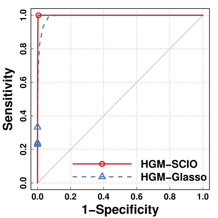
It is difficult compare results with different group assignments $G$. We first consider the true $G$ is given and fixed in our HGM algorithm. That is, we initialize with $G^{\left(0\right)}=G$, and we don’t perform the group update step in Algorithm 1. We compare two methods to estimate the precision matrix $\mathbf{\Omega}$, SCIO and Glasso. Both methods contain a tuning parameter $\lambda$ controlling the sparsity of the matrix, and grids of $50$ values are used in both methods. The network edge identification accuracy with varying $\lambda$ is assessed by the average receiver operating characteristics (ROC), see Figure 4. Overall, the HGM models with both methods, named as HGM-SCIO and HGM-Glasso, have good performance, and HGM-SCIO clearly outperforms HGM-Glasso. When the tuning parameter $\lambda$ is chosen by BIC for both methods, HGM-SCIO has higher sensitivity than HGM-Glasso, while maintaining high specificity as well.

Figure 4: Average receiver operating characteristics on estimating the network edges by embedding SCIO (red solid line) and Glasso (blue dash line) estimators in the HGM algorithm, averaged across 50 runs. The sensitivity and specificity values with the BIC selected $\lambda$ are overlaid by red circles (HGM-SCIO) and blue triangles (HGM-Glasso). HGM-SCIO: HGM with the SCIO estimator in Algorithm (1); HGM-Glasso: HGM with Glasso.

5.2 Group Estimation

To assess the group assignment accuracy, we run all the steps in Algorithm 1 on the simulated data. To fix ideas, we consider 3 values for $\lambda$: $0.1$, $0.2$, and $0.5$. The resulting network connections are dense, moderate, and sparse respectively. For comparing each estimated $\hat{G}$ with the true group $G$, we use the following simple measure, coherence rate,

$$r_{k}=\frac{\max_{i}\left|\hat{G}_{i}\cap G_{k}\right|}{\left|G_{k}\right|},\quad k=1,\dotsc,K.$$

For each run, we initialize with 10 different initial group assignments, and retain the estimated $\hat{G}$ with the largest likelihood. Due to the symmetry of our simulated groups, we pool the coherence measures from different groups across 50 runs. Figure 5 shows that, by the coherence measure, HGM is stable and accurate in group estimation with varying $\lambda$, and $89\%$ of the group estimates equal to the truth exactly.

Figure 5: Boxplots of the coherence rates with varying $\lambda$ over 50 runs for all groups. Over $89\%$ of the coherence rates equal to 1 exactly across all choices of $\lambda$.

6 Discussion

This paper introduces a model for estimating direct connections from large-scale data, motivated by the whole-brain network estimation problem in fMRI. We aim to provide a computationally efficient and interpretable model for data with hundreds of thousands of variables. We propose an alternating update algorithm to estimate the model parameters simultaneously. The model is illustrated using both simulated data and a dataset from a stop/go fMRI experiment.

The interpretation of connections recovered by HGM, however, should be treated with caution. It has been well know than fMRI BOLD signals are confounded by varying hemodynamic processes across the brain, and thus the connectivity should interpreted on the bold level. Moreover, the spatial resolution of fMRI is insufficient for inferring neuronal connections. Thus the connections in HGM should not simply treated as direct neuronal connections, though these can be highly correlated.

There are several possible hypotheses for the voxel grouping in HGM. One may conjecture that smoothness may play a part, and thus nearby voxels are grouped together. However, this simplified explanation does not explain the long-range connections in HGM. We are inclined to hypothesize that the grouping is mostly due to close brain functions. Certainly nearby voxels may share similar brain functions. By grouping, HGM provides two levels of interpretation: how groups are connected to each other, and how brain regions are grouped. It will be interesting to investigate the biological and graph theoretical foundations of these two levels.

The theoretical aspects of HGM are not developed here. Though finite sample theory exists for the precision matrix estimation (Cai et al., 2011; Liu and Luo, 2012), the assumptions are difficult to verify in big data collected from biological experiments (e.g. fMRI). Furthermore, the group assignment is a combinatorial problem, which is difficult to analyze. We, instead, provide the HGM model as a first step to understand large brain networks.

The distribution assumptions can be relaxed. Even if the distribution of $\mathbf{Z}$ has heavier tails, the same convergence rates hold (Cai et al., 2011; Liu and Luo, 2012). More general distributions can be accommodated by nonparametric covariance estimates (Lafferty et al., 2012), which will be interesting to explore in the future.

The independent assumption in $\mathbf{Z}$ can also be replaced with a matrix normal distribution (Leng and Tang, 2012) to describe temporal dependence. In our application example, the whitening step in preprocessing may reduce such dependence. It is also interesting to develop spatio-temporal models to validate this assumption, such as Kang et al. (2012).

Several extensions of HGM are possible. For instance, one may consider modeling the probability of group assignments for each voxel. One may consider studying the group-level HGM from multiple subjects and sessions, either by embedding HGM in mixed models or by the group Lasso penalty (Yuan and Lin, 2006). One may also consider incorporating the distance between voxels to help group assignments, but it should be pointed out that the choice of metric may be challenging. For example, Euclidean distance is usually not a good choice of metric for voxels (Bowman, 2014). We will leave these directions to future research.

7 Proof

The proof of Proposition 2 implies the proof of Proposition 1, and thus the latter is omitted.

The terms in $L$ that are relevant to $\mathbf{Z}$ are, ignoring other factors irrelevant of $\mathbf{Z}$,

$$L_{\mathbf{Z}}=\sum_{k=1}^{K}\sum_{j\in G_{k}}\left\|X_{\cdot j}-Z_{\cdot k}\right\|_{2}^{2}/\left(n\phi_{k}\right)+\frac{1}{n}\operatorname{tr}\left(\mathbf{Z}\mathbf{\Omega}\mathbf{Z}^{T}\right).$$

The derivative of $L_{\mathbf{Z}}$ with respect to $\mathbf{Z}$ is proportional to

$$\mathbf{Z}\mathbf{D}_{G}\mathbf{\Phi}^{-1}+\mathbf{Z}\mathbf{\Omega}-\bar{\mathbf{Z}}\mathbf{D}_{G}\mathbf{\Phi}^{-1}.$$

Multiplying the derivative by $\mathbf{\Phi}$, solve $\mathbf{Z}$ that sets the product zero to yield the minimizer

$$\mathbf{Z}=\bar{\mathbf{Z}}\mathbf{D}_{G}\left[\mathbf{D}_{G}+\mathbf{\Omega}\mathbf{\Phi}\right]^{-1}.$$

Similar to the derivation of the minimizer for $\mathbf{Z}$, the conditional objective function is

$$L_{\mathbf{\Phi}^{-1}}=\frac{1}{n}\sum_{k=1}^{K}\left[\phi_{k}^{-1}\sum_{j\in G_{k}}\left\|X_{\cdot j}-Z_{\cdot k}\right\|_{2}^{2}-\left|G_{k}\right|\log\phi_{k}^{-1}\right].$$

the derivative with respect to $\phi_{k}^{-1}$ equals to, for every $k$,

$$\frac{1}{n}\sum_{j\in G_{k}}\left\|X_{\cdot j}-Z_{\cdot k}\right\|_{2}^{2}-\left|G_{k}\right|\phi_{k}.$$

The solution that sets the derivative to zero is, for every $k$,

$$\phi_{k}=\frac{1}{n\left|G_{k}\right|}\sum_{j\in G_{k}}\left\|Z_{\cdot k}-X_{\cdot j}\right\|_{2}^{2}.$$

Finally, the terms relevant to $\mathbf{\Omega}$ in $L$ are

$$L_{\mathbf{\Omega}}=\frac{1}{n}\operatorname{tr}\left(\mathbf{Z}\mathbf{\Omega}\mathbf{Z}^{T}\right)-\log\det\left(\mathbf{\Omega}\right)+\lambda\left\|\mathbf{\Omega}\right\|_{1},$$

and the minimization is thus equivalent to a Glasso problem on $\mathbf{\Omega}$.

References

- Anderson et al. (2011) Anderson, J. S., Ferguson, M. A., Lopez-Larson, M., and Yurgelun-Todd, D. (2011). Connectivity gradients between the default mode and attention control networks. Brain connectivity, 1(2):147–157.
- Banerjee et al. (2008) Banerjee, O., Ghaoui, L., and d’Aspremont, A. (2008). Model selection through sparse maximum likelihood estimation. Journal of Machine Learning, 9:485–516.
- Beckmann and Smith (2004) Beckmann, C. F. and Smith, S. M. (2004). Probabilistic independent component analysis for functional magnetic resonance imaging. Medical Imaging, IEEE Transactions on, 23(2):137–152.
- Bowman (2014) Bowman, F. D. (2014). Brain imaging analysis. Annual Review of Statistics and Its Application, 1(1):61–85.
- Bowman and Patel (2004) Bowman, F. D. and Patel, R. (2004). Identifying spatial relationships in neural processing using a multiple classification approach. NeuroImage, 23(1):260–268.
- Buckner (2010) Buckner, R. L. (2010). Human functional connectivity: new tools, unresolved questions. Proceedings of the National Academy of Sciences, 107(24):10769–10770.
- Bullmore and Sporns (2009) Bullmore, E. and Sporns, O. (2009). Complex brain networks: graph theoretical analysis of structural and functional systems. Nature Reviews Neuroscience, 10(3):186–198.
- Cai et al. (2011) Cai, T., Liu, W., and Luo, X. (2011). A constrained minimization approach to sparse precision matrix estimation. Journal of the American Statistical Association, 106(494):594–607.
- Calhoun et al. (2001) Calhoun, V., Adali, T., Pearlson, G., and Pekar, J. (2001). A method for making group inferences from functional mri data using independent component analysis. Human brain mapping, 14(3):140–151.
- Chen and Donoho (1994) Chen, S. and Donoho, D. (1994). Basis pursuit. In Conference Record of the Twenty-Eighth Asilomar Conference on Signals, Systems and Computers, volume 1, pages 41–44.
- Chiang-shan et al. (2010) Chiang-shan, R. L., Morgan, P. T., Matuskey, D., Abdelghany, O., Luo, X., Chang, J. L., Rounsaville, B. J., Ding, Y.-s., and Malison, R. T. (2010). Biological markers of the effects of intravenous methylphenidate on improving inhibitory control in cocaine-dependent patients. Proceedings of the National Academy of Sciences, 107(32):14455–14459.
- Dempster (1972) Dempster, A. P. (1972). Covariance selection. Biometrics, pages 157–175.
- Duann et al. (2009) Duann, J.-R., Ide, J. S., Luo, X., and Li, C.-s. R. (2009). Functional connectivity delineates distinct roles of the inferior frontal cortex and presupplementary motor area in stop signal inhibition. The Journal of Neuroscience, 29(32):10171–10179.
- Eloyan et al. (2013) Eloyan, A., Crainiceanu, C. M., and Caffo, B. S. (2013). Likelihood-based population independent component analysis. Biostatistics, 14(3):514–527.
- Fair et al. (2007) Fair, D. A., Schlaggar, B. L., Cohen, A. L., Miezin, F. M., Dosenbach, N. U., Wenger, K. K., Fox, M. D., Snyder, A. Z., Raichle, M. E., and Petersen, S. E. (2007). A method for using blocked and event-related fmri data to study r̈esting statef̈unctional connectivity. Neuroimage, 35(1):396–405.
- Forgy (1965) Forgy, E. (1965). Cluster analysis of multivariate data: Efficiency versus interpretability of classifications. Biometrics, 21:768–769.
- Friedman et al. (2008) Friedman, J., Hastie, T., and Tibshirani, R. (2008). Sparse inverse covariance estimation with the graphical lasso. Biostatistics, 9(3):432–441.
- Friston et al. (2003) Friston, K., Harrison, L., and Penny, W. (2003). Dynamic causal modelling. NeuroImage, 19(4):1273 – 1302.
- Friston (2011) Friston, K. J. (2011). Functional and effective connectivity: a review. Brain connectivity, 1(1):13–36.
- Friston et al. (1994) Friston, K. J., Holmes, A. P., Worsley, K. J., Poline, J.-P., Frith, C. D., and Frackowiak, R. S. (1994). Statistical parametric maps in functional imaging: a general linear approach. Human brain mapping, 2(4):189–210.
- Goutte et al. (1999) Goutte, C., Toft, P., Rostrup, E., Nielsen, F. Å., and Hansen, L. K. (1999). On clustering fmri time series. NeuroImage, 9(3):298–310.
- Guimera and Amaral (2005) Guimera, R. and Amaral, L. A. N. (2005). Functional cartography of complex metabolic networks. Nature, 433(7028):895–900.
- Guo (2011) Guo, Y. (2011). A general probabilistic model for group independent component analysis and its estimation methods. Biometrics, 67(4):1532–1542.
- Hartigan and Wong (1979) Hartigan, J. A. and Wong, M. A. (1979). Algorithm as 136: A k-means clustering algorithm. Journal of the Royal Statistical Society. Series C (Applied Statistics), 28(1):100–108.
- Hsieh et al. (2013) Hsieh, C.-J., Sustik, M. A., Dhillon, I., Ravikumar, P., and Poldrack, R. (2013). Big & quic: Sparse inverse covariance estimation for a million variables. In Advances in Neural Information Processing Systems, pages 3165–3173.
- Jakab et al. (2012) Jakab, A., Molnár, P. P., Bogner, P., Béres, M., and Berényi, E. L. (2012). Connectivity-based parcellation reveals interhemispheric differences in the insula. Brain Topography, 25(3):264–271.
- Kang et al. (2012) Kang, H., Ombao, H., Linkletter, C., Long, N., and Badre, D. (2012). Spatio-spectral mixed-effects model for functional magnetic resonance imaging data. Journal of the American Statistical Association, 107(498):568–577.
- Kelly et al. (2012) Kelly, C., Toro, R., Di Martino, A., Cox, C. L., Bellec, P., Castellanos, F. X., and Milham, M. P. (2012). A convergent functional architecture of the insula emerges across imaging modalities. Neuroimage, 61(4):1129–1142.
- Lafferty et al. (2012) Lafferty, J., Liu, H., and Wasserman, L. (2012). Sparse nonparametric graphical models. Arxiv preprint arXiv:1201.0794.
- Lauritzen (1996) Lauritzen, S. L. (1996). Graphical models. Oxford University Press.
- Lehmann and Casella (1998) Lehmann, E. L. and Casella, G. (1998). Theory of point estimation, volume 31. Springer.
- Leng and Tang (2012) Leng, C. and Tang, C. Y. (2012). Sparse matrix graphical models. Journal of the American Statistical Association, 107(499):1187–1200.
- Liu and Luo (2012) Liu, W. and Luo, X. (2012). High-dimensional sparse precision matrix estimation via sparse column inverse operator. arXiv preprint arXiv:1203.3896.
- Lloyd (1982) Lloyd, S. (1982). Least squares quantization in pcm. Information Theory, IEEE Transactions on, 28(2):129–137.
- Luo et al. (2012) Luo, X., Small, D., Li, C., and Rosenbaum, P. (2012). Inference with interference between units in an fmri experiment of motor inhibition. Journal of the American Statistical Association, 107(498):530–541.
- Luo et al. (2013) Luo, X., Zhang, S., Hu, S., Bednarski, S. R., Erdman, E., Farr, O. M., Hong, K.-I., Sinha, R., Mazure, C. M., and Chiang-shan, R. L. (2013). Error processing and gender-shared and-specific neural predictors of relapse in cocaine dependence. Brain, 136(4):1231–1244.
- MacQueen et al. (1967) MacQueen, J. et al. (1967). Some methods for classification and analysis of multivariate observations. In Proceedings of the fifth Berkeley symposium on mathematical statistics and probability, volume 1, page 14. California, USA.
- Meinshausen and Bühlmann (2006) Meinshausen, N. and Bühlmann, P. (2006). High-dimensional graphs and variable selection with the lasso. The Annals of Statistics, 34(3):1436–1462.
- Pelleg et al. (2000) Pelleg, D., Moore, A. W., et al. (2000). X-means: Extending k-means with efficient estimation of the number of clusters. In ICML, pages 727–734.
- Power et al. (2013) Power, J. D., Schlaggar, B. L., Lessov-Schlaggar, C. N., and Petersen, S. E. (2013). Evidence for hubs in human functional brain networks. Neuron, 79(4):798–813.
- Sauvage et al. (2011) Sauvage, C., Poirriez, S., Manto, M., Jissendi, P., and Habas, C. (2011). Reevaluating brain networks activated during mental imagery of finger movements using probabilistic tensorial independent component analysis (tica). Brain imaging and behavior, 5(2):137–148.
- Seeley et al. (2007) Seeley, W. W., Menon, V., Schatzberg, A. F., Keller, J., Glover, G. H., Kenna, H., Reiss, A. L., and Greicius, M. D. (2007). Dissociable intrinsic connectivity networks for salience processing and executive control. The Journal of neuroscience, 27(9):2349–2356.
- Simmonds et al. (2008) Simmonds, D. J., Pekar, J. J., and Mostofsky, S. H. (2008). Meta-analysis of go/no-go tasks demonstrating that fmri activation associated with response inhibition is task-dependent. Neuropsychologia, 46(1):224–232.
- Smith et al. (2011) Smith, S. M., Miller, K. L., Salimi-Khorshidi, G., Webster, M., Beckmann, C. F., Nichols, T. E., Ramsey, J. D., and Woolrich, M. W. (2011). Network modelling methods for fmri. Neuroimage, 54(2):875–891.
- Smith et al. (2013) Smith, S. M., Vidaurre, D., Beckmann, C. F., Glasser, M. F., Jenkinson, M., Miller, K. L., Nichols, T. E., Robinson, E. C., Salimi-Khorshidi, G., Woolrich, M. W., et al. (2013). Functional connectomics from resting-state fmri. Trends in cognitive sciences, 17(12):666–682.
- Sporns (2014) Sporns, O. (2014). Contributions and challenges for network models in cognitive neuroscience. Nature Neuroscience.
- Tibshirani (1996) Tibshirani, R. (1996). Regression shrinkage and selection via the lasso. Journal of the Royal Statistical Society. Series B (Methodological), 58(1):267–288.
- Turk-Browne (2013) Turk-Browne, N. B. (2013). Functional interactions as big data in the human brain. Science, 342(6158):580–584.
- Tzourio-Mazoyer et al. (2002) Tzourio-Mazoyer, N., Landeau, B., Papathanassiou, D., Crivello, F., Etard, O., Delcroix, N., Mazoyer, B., and Joliot, M. (2002). Automated anatomical labeling of activations in spm using a macroscopic anatomical parcellation of the mni mri single-subject brain. Neuroimage, 15(1):273–289.
- Varoquaux and Craddock (2013) Varoquaux, G. and Craddock, R. C. (2013). Learning and comparing functional connectomes across subjects. NeuroImage, 80:405–415.
- Xue et al. (2008) Xue, G., Aron, A. R., and Poldrack, R. A. (2008). Common neural substrates for inhibition of spoken and manual responses. Cerebral Cortex, 18(8):1923–1932.
- Yuan (2010) Yuan, M. (2010). High dimensional inverse covariance matrix estimation via linear programming. Journal of Machine Learning Research, 11:2261–2286.
- Yuan and Lin (2006) Yuan, M. and Lin, Y. (2006). Model selection and estimation in regression with grouped variables. Journal of The Royal Statistical Society Series B, 68:49–67.
- Yuan and Lin (2007) Yuan, M. and Lin, Y. (2007). Model selection and estimation in the gaussian graphical model. Boimetrika, 94(1):19–35.
- Zhang et al. (2012) Zhang, S., Ide, J. S., and Chiang-shan, R. L. (2012). Resting-state functional connectivity of the medial superior frontal cortex. Cerebral Cortex, 22(1):99–111.
- Zhang and Li (2014) Zhang, S. and Li, c.-s. R. (2014). Functional clustering of the human inferior parietal lobule by whole brain connectivity mapping of resting state fmri signals. Brain connectivity, In Press.