Dispersal limitation and roughening of the ecological interface

ANDREW J. ALLSTADT,^1,⋄,⋆ JONATHAN A. NEWMAN,^2,§ JONATHAN A. WALTER,^3,♯ G. KORNISS,^4,‡ and THOMAS CARACO^5,†

1. Blandy Experimental Farm, University of Virginia, Boyce VA 22620, USA

2. School of Environmental Sciences, University of Guelph, Guelph, Ontario N1G 2W1, Canada

3. Department of Environmental Sciences, University of Virginia, Charlottesville, VA 22904-4123, USA

4. Department of Physics, Applied Physics, and Astronomy,
Rensselaer Polytechnic Institute, 110 8th Street, Troy NY 12180-3590, USA

5. Department of Biological Sciences, University at Albany, Albany NY 12222, USA

^⋄Present Address: Department of Forest and Wildlife Ecology, University of Wisconsin-Madison, Madison WI 53706, USA

^⋆Corresponding author, e-mail: allstadt@wisc.edu; ^§e-mail: jonathan.newman@uoguelph.ca; ^♯e-mail: jaw3es@virginia.edu; ^‡e-mail:korniss@rpi.edu; ^†e-mail: tcaraco@albany.edu.

Keywords: ecological invasion, front-runner, interface dynamics, scaling laws, spatial competition, stochastic roughening

Abstract. Limited dispersal distance, whether associated with vegetative growth or localized reproduction, induces spatial clustering and, in turn, focuses ecological interactions at the neighborhood scale. In particular, most invasive plants are clonal, cluster through vegetative propagation, and compete locally. Dispersal limitation implies that invasive spread occurs as advance of an ecological interface between invader and resident species. Interspecific competition along the interface produces random variation in the extent of invasive growth. Development of these random fluctuations, termed stochastic roughening, will often structure the interface as a self-affine fractal; a series of power-law scaling relationships follows as a result. For a diverse array of local growth processes exhibiting both forward and lateral propagation, the extent of invader advance becomes spatially correlated along the interface, and the width of the interface (the area where invader and resident compete directly) increases as a power function of time. Once roughening equilibrates statistically, interface width and the location of the most advanced invader (the “front-runner”) beyond the mean incursion should both increase as a power function of interface length. To test these predictions, we let white clover (Trifolium repens) invade ryegrass (Lolium perenne) experimentally. Spatial correlation developed as anticipated, and both interface width and the front-runner’s lead scaled as a power law of length. However, the scaling exponents differed, likely a consequence of clover’s growth morphology. The theory of kinetic roughening offers a new framework for understanding causes and consequences of spatial pattern in between-species interaction, and indicates when interface measures at a local scale predict properties of an invasive front at extended spatial scales.

Pattern analysis of plant communities commonly reveals spatial mosaics generated by clustered growth of individual species [Cain et al. 1995, Dale 1999, Condit et al. 2000]. Clustering may follow a template set by environmental heterogeneity, especially if different locations favor different species [Snyder and Chesson 2003], but more often, strong dispersal limitation aggregates conspecific individuals [Harada and Iwasa 1994]. For example, most invasive plants are clonal and propagate vegetatively [Kolar and Lodge 2001, Sakai et al. 2001, Liu et al. 2006], so that invaders will initially cluster among residents [Korniss and Caraco 2005, Cantor et al. 2011].

Spatial clustering influences frequencies of different biotic interactions and the consequent population dynamics [Herben et al. 2000]. Individual plants usually compete at the nearest-neighbor scale [Goldberg and Barton 1992, Levine et al. 2004]. Therefore, when different species each aggregate spatially and interact locally, intraspecific competition should predominate within clusters, while interspecific competition will localize at the interface between clusters [Chesson 2000, Yurkonis and Meiners 2004]. The resulting interaction geometry implies that the advance versus extinction of a rare competitor may depend on development and motion of a between-species interface [Gandhi et al. 1999, Allstadt et al. 2009, O’Malley et al. 2010]. That is, we envision a non-equilibrium system where increase (decrease) in a species’ abundance drives interface motion. The dynamics of an ecological interface distinguishes it from an ecotone, when the latter implies a change in species composition due to abiotic factors that vary slowly relative to the timescale of population growth [Gastner et al. 2009, Eppinga et al. 2013].

A focal species’ density declines from positive equilibrium to rarity across the width of an ecological interface. For clarity, we refer to the focal species as the invader, so that invasive movement of the interface (or advancing front) implies increase in the area occupied by the focal species. Given this simple, general picture, we ask how varying the length of the interface affects statistical properties of an invader-resident interaction. We emphasize the relative position of the “front-runner,” the furthest advanced invader, a metric used in both theoretical and applied invasion ecology [Hajek et al. 1996, Clark et al. 2001, Thomson and Ellner 2003].

To begin, we assume invasive advance is a dispersal-limited, stochastic process and treat the ecological interface as a self-affine fractal, which implies that both interface width and the front-runner’s lead will depend on the length of the advancing front [O’Malley et al. 2006, O’Malley et al. 2009a]. Second, we report an experiment testing our predictions at a local scale; we let Dutch white clover (Trifolium repens) advance into plots of perennial ryegrass (Lolium perenne). Our contribution lies in the application of scaling laws, drawn from the theory of kinetic roughening [Family and Vicsek 1985, Barabási and Stanley 1995], as a framework for understanding spatial-growth patterns. We help clarify how interface roughening organizes biotic interactions of locally clustered species. More generally, the concepts we invoke may help integrate spatial-growth processes across quite different length scales.

LOCAL DISPERSAL and INTERFACE ROUGHENING

Consider a spatially aggregated invader advancing into an area occupied by a resident species. As the dispersal-limited invader’s abundance increases from rarity, it displaces the resident along the interface. Deterministic reaction-diffusion models, which assume continuous densities, cannot appreciate observable consequences of spatially correlated variability along a front generated by advance of a locally dispersing species [Clark et al. 2003, Antonovics et al. 2006, O’Malley et al. 2009b]. But discrete (“individual-based”) models may capture effects of the nonlinearity and stochasticity inherent to the dynamics of rarity at an ecological interface [Durrett and Levin 1994, Pachepsky and Levine 2011]. Therefore, we characterize interface roughening, and motivate our experiment, in the context of a discrete, stochastic process where an invader and a resident compete for space [Allstadt et al. 2012]. For commentary on discrete versus continuous-density models, see Moro [2003] or van Saarloos [2003]; Appendix A summarizes differences between these models.

In a two-dimensional environment, development of spatially correlated growth along an interface is termed stochastic roughening [Kardar et al. 1986, Plischke et al. 1987, Barabási and Stanley 1995]. Roughening and dynamic scaling offer a conceptual framework for identifying dynamics shared by correlated growth processes differing in details of local interactions. Applications span growth processes in physical materials [Barabási and Stanley 1995], biological tissues, including tumors [Brú et al. 2003, Galeano et al. 2003], parallel-computing and information systems [Korniss et al. 2000, Korniss et al. 2003], and in ecological invasion [O’Malley et al. 2006, O’Malley et al. 2009a]. When we analyze the front-runner’s location, correlated fluctuations along the interface are particularly important, since traditional extreme-value statistics [Fisher and Tippett 1928, Galambos et al. 1994], developed for independent random variables, do not apply [Majumdar and Comtet 2004]. Figure 1 shows an advancing, roughening interface from the field experiment we report below. The invader’s advance along the interface clearly roughens with time. The figure also suggests correlated advance at nearby locations.

Figure 1: White clover (T. repens, black area) advancing into perennial ryegrass (L. perenne), from photographs taken during experiment. Interface length $L$$\equiv$$L_{y}$$=$$16~{}m$. June (left), August (center) and October (right) 2010 shown. The interface advances, left to right, and roughens; neighboring heights suggest spatial correlation.

Interface roughening: development and saturation

After defining attributes of the interface, we describe a roughened front‘s development. Then we address roughening at statistical equilibrium (termed “saturation”). Table 1 lists model symbols.

Symbols	Definitions
$L_{x},\;L_{y}(=L)$	Lattice size ($L=$ interface length = front length)
${\rm\bf{r}}$	Lattice site
$t$	time
$h_{y}(t)$	Rightmost invader in row $y$ at time $t$
$\overline{h}(t)$	Mean of $h_{y}(t)$ (the average is taken across all rows $y$)
$h_{max}(t)$	Rightmost invader at time $t$
$\Delta_{max}(t)=h_{max}(t)-\overline{h}(t)$	Distance from front-runner to mean of front
$v^{*}$	Asymptotic velocity of invasive advance
$\langle w^{2}\rangle$	Mean squared interface width
$\xi(t)$	Correlation length along interface
$t_{\times}$	Crossover time, where $w^{2}$ equilibrates
$\alpha$	Roughness exponent
$\beta$	Growth exponent
$z$	Dynamic exponent

Table 1: Definitions of variables.

An $L_{x}$$\times$$L_{y}$ rectangular lattice represents a habitat occupied by the resident and invader species. Each lattice site is either occupied by the invader, occupied by the resident, or is empty. Mortality opens occupied sites. An empty site $\bf{r}$ becomes occupied through propagation from an occupied site among the nearest neighbors of $\bf{r}$. Typical neighborhoods include only the 4 or 8 closest sites; restricting propagation to nearest neighbors, of course, imposes dispersal-limitation. We assume that the invader’s competitive superiority drives interface motion.

Suppose that the invader initially occupies only a few vertical columns at the left edge of the lattice, and the resident occupies all other sites. Invasive advance occurs in the $x$-direction. Importantly, neighborhood geometry (the dispersal constraint) permits both forward and lateral growth. The former pushes the front, and the latter generates spatial correlation along the front [Kardar et al. 1986, Barabási and Stanley 1995]. That is, lateral growth of advanced heights tends to increase height in adjacent rows.

We let $L\equiv L_{y}$, interface length (hence, front length). At time $t$, $h_{y}(t)$ is the location of the most advanced (right-most) invader in row $y$; $y=1,2,...,L$. The front’s average location is the mean height among rows, $\overline{h}(t)=\sum_{y}h_{y}(t)/L$. We take longitudinal system size $L_{x}$ as sufficiently large that it does not affect population processes.

Figure 2 shows the width of the interface about the invader’s average incursion $\overline{h}(t)$. To quantify roughening, we define the width of the interface via:

$$w^{2}(L,t)=\frac{1}{L}\sum_{y=1}^{L}[h_{y}(t)-\overline{h}(t)]^{2}\;$$ (1)

Roughness $w^{2}(L,t)$ itself varies stochastically, and we represent its expectation (averaged over realizations of intrinsic noise) at time $t$ by $\langle w^{2}(L,t)\rangle$. We take $w=\sqrt{\langle w^{2}(L,t)\rangle}$ as the width of the front, the typical extent of the interface parallel to the direction of advance.

Next, we identify power-law scaling relationships that should characterize the structure of an interface with spatially correlated heights. Importantly, these qualitative relationships do not, in general, depend on details of the ecological interactions shaping the interface. Numerical calibration of the scaling laws can, of course, differ across species and environments.

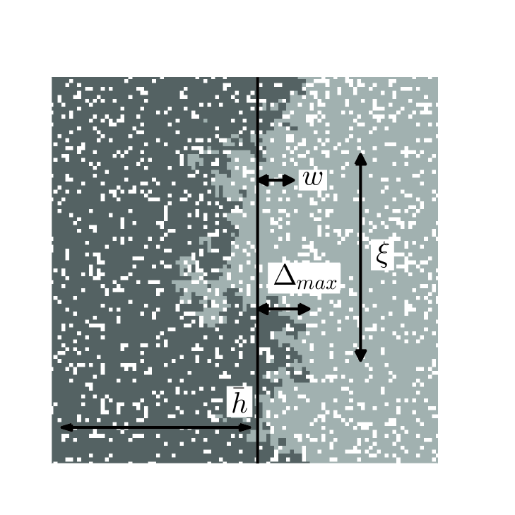
Figure 2: Width ($w$) and the extreme advance ($\Delta_{max}$) relative to the mean front position ($\overline{h}$) in a rough front. For illustration, correlation length $\xi$ is also indicated. Dark: invader, medium: resident and white: open. Figure generated by simulation of model in O’Malley et al. (2006).

Interface development. – Assume a linear front at time $t=0$, a flat initial interface. As the invader begins to advance, the interface starts to roughen, and invader heights $h_{y}(t)$ become dependent random variables. That is, a single correlation length $\xi(t)$ develops along the interface (Fig. 2). Correlation length initially increases with time according to the power-law scaling $\xi(t)\sim t^{1/z}$ [Majumdar and Comtet 2005], where $z$ is called the dynamic exponent. But once $\xi(t)$ spans the length $L$ of the interface, “crossover” occurs. The interface continues to advance, but roughening reaches statistical equilibrium when spatial correlation spans the length of the interface (roughening “saturates” at crossover) [Barabási and Stanley 1995]. The duration of interface development, termed crossover time $t_{\times}$, increases with interface length; the power-law scaling is $t_{\times}\sim L^{z}$. The development of interface width offers a more easily tested prediction. Prior to saturation, interface width $w$ exhibits temporal scaling behavior according to $w\sim t^{\beta}$. $\beta$ $(\beta>0)$ is called the growth exponent [O’Malley et al. 2006].

We monitor increasing correlation distance along the developing interface in two ways; each combines results from windows of length $l<L$. The local width, $w_{t}(l)$, is the expected interface width estimated for the portion of the interface with length $l$, at time $t$. The height-difference correlation function [Karabacak et al. 2001] integrates roughness during both development and saturation. The height-difference correlation function, at time $t$, is given by:

$$C_{t}(l)=\left\langle\left(h_{y+l}(t)-h_{y}(t)\right)^{2}\right\rangle_{y}^{1/2}$$ (2)

where $t>0$ and the average is taken across all rows $y$. Similarly, we define the height-height correlation function (the Pearson correlation):

$$G_{t}(l)=\frac{\left\langle\left(h_{y+l}(t)-\overline{h}(t)\right)\left(h_{y}(t)-\overline{h}(t)\right)\right\rangle_{y}^{1/2}}{\left\langle\left(h_{y}(t)-\overline{h}(t)\right)^{2}\right\rangle_{y}^{1/2}}\;.$$ (3)

We use $G_{t}(l)$ to estimate correlation length $\xi(t)$; height-height correlation should decline as distance between rows increases.

For $l<\xi(t)$, both $w_{t}(l)$ and $C_{t}(l)$ exhibit power-law scaling over distances along the interface: $w_{t}(l),~{}C_{t}(l)\sim l^{\alpha}$. $\alpha$ $(\alpha>0)$ is the roughness exponent, and characterizes the fractal nature of the interface. As the interface roughens with time, the correlation distance $\xi$ increases. Consequently, the linear dependence of $\ln w_{t}(l)$ and $\ln C_{t}(l)$ on $\ln l$, with slope $\alpha$, should extend to greater lengths $l$ along the interface, until saturation.

The saturated interface. – After crossover $(t>t_{\times})$, steady-state properties of the interface depend on its length $L$ [Schehr and Majumdar 2006]. Interface width $w$ scales with interface length according to $\langle w^{2}(L,\infty)\rangle$$\sim$$L^{2\alpha}$. That is, interface width increases as a power function of its length, according to the roughness exponent $\alpha$.

Note that we do not predict the value of roughness per se, but ask how roughening changes from a shorter to a longer interface, or from portions of an interface to its entire length [O’Malley et al. 2009a]. The power-law scaling for $\langle w^{2}(L,\infty)\rangle$ does not imply that clonal plants with a guerilla/runner morphology will be rougher at their growth interface than will clonal plants with a phalanx morphology. Rather, the scaling relationship implies that if we can estimate interface roughening across local spatial scales, we can predict the way interface roughening increases at greater length scales.

In general, the scaling exponents are interdependent: $\alpha=\beta z$ [Kardar et al. 1986]; see Appendix B. The dependence arises when the interface has a self-affine structure. Geometrically, we begin with a one-dimensional interface embedded in a two-dimensional environment; random demographic events render the interface disorderly, and we assume that the interface equilibrates as an anisotropic fractal [Barabási and Stanley 1995]. “Random demographic events” means local processes that include both forward and lateral invader growth. As noted above, forward growth pushes invasive advance, and lateral growth builds spatial correlations between heights. Without lateral growth, each $h_{y}(t)$ becomes an independent birth-death process; independence implies, of course, lack of spatial correlation. “Anisotropic fractal” implies a self-affine interface and an associated roughness exponent. Consider the interface width $w(L)$. Suppose that we increase interface length according to $L\rightarrow kL$. Then the width must be re-scaled according to $w\rightarrow k^{\alpha}w$ to preserve statistical invariance (“look the same”); under anisotropic transformation, height and interface length must be increased by different factors.

Roughening, scaling and the front-runner

Interface velocity. – Analytic approximation of a discrete, stochastic model’s asymptotic interface velocity $v^{*}$ remains a challenge [Pechenik and Levine 1999], especially for two-dimensional environments. Dispersal limitation reduces velocity, compared to the corresponding reaction-diffusion model [Moro 2001, Escudero et al. 2004]. Krug and Meakin (1990) found that a discrete model’s reduction in velocity, relative to the reaction-diffusion wave-speed, varies inversely with interface length. Unfortunately, the exact reduction depends on the particular model’s local dynamics. That is, the manner in which velocity increases with $L$, as well as the asymptotic velocity $v^{*}$ itself, depend on details governing local (i.e., individual-level) propagation and mortality.

Importantly, the scaling laws involving the roughness exponent $\alpha$ do not depend on invasion speed [Barabási and Stanley 1995]. This includes the probability distribution of the front-runner’s lead. However, this does not imply that velocity cannot be influenced by variation in roughness (see Discussion).

The front-runner: scaling of extremes. – The maximal invasive advance defines the front-runner’s position. At time $t$ we locate the front-runner at $h_{max}(t)=\max_{y}\{h_{y}(t)\}$. Given mean interface height $\overline{h}(L,t)$, the invader’s maximal relative advance at time $t$ is $\Delta_{max}(L,t)=h_{max}(t)-\overline{h}(L,t)$. We assume that roughening equilibrates before considering the scaling of the expected lead $\langle\Delta_{max}\rangle_{L}$; note dependence on interface length $L$.

The probability density of the front-runner’s excess $\Delta_{max}(L,t)$ has been obtained analytically [Majumdar and Comtet 2004, Majumdar and Comtet 2005]. For broad classes of dispersal-limited stochastic growth models, the scaled variable $\Delta_{max}/\langle\Delta_{max}\rangle$ has an Airy probability density, and the steady-state average excess of the front-runner over the mean height scales with interface length exactly as does the width. That is, $\langle\Delta_{max}\rangle_{L}\sim L^{\alpha}$ [O’Malley et al. 2009a]. Furthermore, we can infer the size of the extremes for an interface of linear size $L$ with estimates obtained in limited observation windows with size $L_{\rm{obs}}$. We have: $\langle\Delta_{max}(L)\rangle\approx\langle\Delta_{max}(L_{\rm{obs}})\rangle k^{\alpha}$, where $k=(L/L_{\rm{obs}})$, by the properties of a self-affine interface. Table 2 collects scaling relationships we study; for a graphical summary of interface-roughness scaling, see Appendix B.

Regime	Prediction	Comment
Development	$\xi(t)\sim t^{1/z}$	Correlation length, dynamic exponent
	$w_{t}\sim t^{\beta}$	Interface width, growth exponent
	$t_{\times}\sim L^{z}$	Crossover time, interface length
	$C_{t}(l)\sim l^{\alpha}$	Height-difference correlation, $l<\xi(t)$
Stationarity	$w\sim L^{\alpha}$	Interface width, roughness exponent
	$\langle\Delta_{max}\rangle_{L}\sim L^{\alpha}$	Front-runner’s lead
	$\beta=\alpha/z$	Self-affine fractal

Table 2: Predicted scaling relationships. The interface roughens during development. After spatial correlation spans interface length, interface width remains statistically stationary.

AN EXPERIMENTAL INTERFACE

To evaluate interface scaling, we studied dispersal-limited competition between Dutch white clover (T. repens) and perennial ryegrass (L. perenne). Both species reproduce mainly through local, clonal growth [Turkington et al. 1979, Schwinning and Parsons 1996a]. T. repens propagates vegetatively through stoloniferous stems [Fraser 1989], while L. perenne produces tillers [Fustec et al. 2005]. Biotic interactions, including competition, between these important forage crops are well understood [Cain et al. 1995, Schwinning and Parsons 1996b]. We located experimental plots at the University of Guelph Turfgrass Institute in an area homogeneous with respect to micro-topography ($43^{\circ}33^{\prime}N,80^{\circ}13^{\prime}W$). To minimize spatial heterogeneity, vegetation and top layer of soil were removed, and the soil tilled before the experiment began.

We established plots with interface length $L=$ 1, 2, 4, 8, and 16 $m$, with four replicates of each length. To avert edge effects, we added a $0.5~{}m$ buffer, where no data were collected, at both ends of every plot. Each plot had a total height of $3~{}m$, and was initially split lengthwise by plastic dividers into sections of $1~{}m$ and the remaining $2~{}m$. We planted T. repens in the one-meter sections, and L. perenne in the two meter sections; we anticipated that clover would advance, given the soil resources and occasional mowing. Appendix C details experimental methods.

By spring 2009 mono-cultures were well established, and we removed the plastic barriers between species. In June 2010 we began recording the advance of T. repens in each plot monthly. We resolved measurements at a scale of $1~{}cm^{2}$, the approximate size of an individual clover ramet [Silvertown 1981]. We marked each $1~{}m^{2}$ subsection of every plot permanently, to reference growth measurements. Each such subsection was photographed from above after mowing each month. We re-projected each photo to correct for perspective, and combined photos from the same plot. We recorded row heights $h_{y}(t)$ for T. repens in each plot, and noted the front-runner’s lead on the mean clover height.

We tested power-law relationships against alternative linear and exponential models [Solow et al. 2003]. Additionally, we fit the power-law models with two different assumptions regarding error distribution. The first assumed normally distributed, additive error; the second assumed log-normally distributed, multiplicative error [Xiao et al. 2011]. Our scaling laws, Table 2, predict the latter form. We compared relative support for each model using differences in AIC scores ($\Delta AIC$); we considered models with $\Delta AIC<2$ as supported substantially [Burnham and Anderson 2002].

Results

During the 2010 growing season, clover advanced rapidly; several longer fronts approached the far end of the plot by October. Figure 3A shows each plot’s mean height $\overline{h}(t)$ against time. Overall mean clover height increased for five consecutive months. However, several clover fronts began to experience winter die-back in October. Therefore, our analysis treated data from June through August as the interface-development period, and treated data from September (month 4) as stationary. This is an approximation, since correlation lengths for larger values of $L$ continued to grow during October.

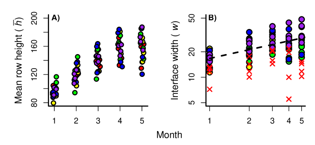
Figure 3: Experimental interface development. A. Mean plot heights ($cm$) by month. Red, yellow, green, blue, and purple indicate, respectively, $L=1,2,4,8,16~{}m$. “Noise” added to abscissa for visibility. B. Each plot’s interface width by month; note the logarithmic scale of the abscissa. Dashed line indicates scaling of the first 4 months (development). Estimated growth exponent $\beta=0.31$. $1~{}m$ plots marked as X, signifying earlier saturation; see text.

Interface development. – Spatial correlations between row heights $h_{y}(t)$ both increased in strength and extended to greater distances along the interface as clover advanced. Since development of correlation length should not depend on $L$, we pooled observations from all plots. We estimated correlation $G_{t}(l)$ between row heights $h_{y}(t)$, as a function of distance, for each of the five months. Figure 4A shows the resulting correlogram; spatial correlation increased every month across most distances less than 200 $cm$.

The height-difference correlation $C_{t}(l)$ also revealed that correlation distance $\xi(t)$ increased during interface development. More importantly, the distance $l$ ($l<\xi(t)$) over which $C_{t}(l)$ scaled as a power-law increased each month; see Figure 4B. The scaling of the height-difference correlation depends on the roughness exponent $\alpha$, since $C\sim l^{\alpha}$ for $l<\xi(t)$. Using the result for month 4, our model selection procedure strongly supported a power-law relationship with multiplicative error (Table 3). Regression analysis of the $C_{t}(l)$ results yielded an estimate of the roughening exponent as $\alpha=0.277\pm 0.002$; see Figure 4B.

During interface development, the temporal increase in roughening should scale such that $\langle w^{2}(L,t)\rangle$$\sim$$t^{2\beta}$. Figure 3B shows each plot’s interface width against time. We first tested the predicted scaling after excluding data from plots with $L=1~{}m$, since roughening in those plots equilibrated earlier than was the case for larger $L$. Our model selection procedure found support for the power-law model with multiplicative log-normal error (Table 3). Using this model, we estimated the growth exponent $\beta$ as 0.34 $\pm$ 0.12 (mean $\pm$ 95% confidence interval; $R^{2}=0.355$). Including the plots where $L=1~{}m$ had little effect, producing an estimate $\beta$ = 0.313; see Figure 3B. In parallel, Figure 4C shows how scaling of the local interface widths $w_{t}(l)$ developed through time.

Velocity. – After saturation, we anticipated that velocity would increase with interface length. August-to-September velocities (differences in mean monthly clover heights) were all positive, but independent of interface length $L$. Interestingly, the greatest overall mean velocity occurred during the first month of growth. As the growing season ended in September, longer fronts continued to advance, but some shorter fronts receded.

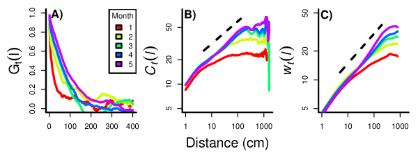
Figure 4: Field experiment: interface development. A. Spatial correlogram: correlation of row heights, $G_{t}(l)$ [Eq. (3)]. The strength and lag distance at which correlations $G_{t}(l)$ remained significant increased through time, indicating an increase in the correlation length, $\xi(t)$, along the interface. Key indicates month 1 through 5 for each plot. B. Height-difference correlation function, $C_{t}(l)$ [Eq. (2)], for months 1 through 5. Distance over which power-law scaling holds increases with time, that is, increases as correlation distance increases. Dashed line indicates month-4 scaling: $\alpha=0.277$. C. Local interface width $w_{t}(l)$ across months. The dashed line indicates the scaling relationship for month 4, based on the estimated growth exponent ($\beta$) of 0.34.

Stationary roughness and the front-runner: power laws. – We assume that roughening equilibrated in month 4. We tested the predicted scaling against alternative models in two ways. The first invokes the local roughening analysis, restricted to the final month’s data. The second estimates how mean interface width increases with $L$.

After saturation, the local width $w(l)$, where $(l\leq L)$, should scale as $w(l)\sim l^{\alpha}$. We combined month-4 data from different plots to characterize local roughening; see Figure 4C. Our AIC-criterion strongly supported the power-law formulation with multiplicative error (Table 3). The associated estimate of the roughness exponent was $\alpha=0.311\pm 0.002$. Our mean roughening analysis treated each plot’s width $w(L)$ separately. Using estimates from September (see Figure 5A), the model selection procedure again provided substantial support for a power-law relationship with multiplicative error (Table 3). The power-law model for mean roughening as a function of interface length $L$ led us to estimate $\alpha$ as $0.278\pm 0.18$.

Once roughening has equilibrated, the average lead of the front-runner, beyond the mean interface height, should scale with length as $\langle\Delta_{max}\rangle_{L}\sim L^{\alpha}$. Our model selection procedure once again found support for power-law scaling with multiplicative error (Table 3), the form predicted. Using the preferred model, we estimated the roughening exponent as $\alpha=0.475\pm 0.19$; $R^{2}=0.6$; see Fig. 5B.

Figure 5: Saturated roughening and the front-runner. A. Interface widths ($cm$)for different front lengths $L$, data from September (month 4). Dashed line indicates power-law scaling. B. Front-runner’s exceedance $(\Delta_{max})$, in $cm$, for different interface lengths $L$, data from month 4. Dashed line indicates power-law scaling.

Clover Growth Analysis	Linear	Exp 1	Exp 2	Pow 1	Pow 2
Dynamic $w^{2}(t)$	411.21	407.82	4.65	0	408.72
$C(l)$	2014.94	1716.08	754.1	0	1398.53
$w^{2}(l)$	3629.0	3061.25	1528.87	0	2528.99
$w^{2}(L)$	118.44	117.02	2.56	0	117.18
$\langle\Delta_{max}\rangle_{L}$	158.15	155.15	6.48	0	155.76

Table 3: $\Delta AIC$ scores. Models compared are as follows. Linear: $y=x+\epsilon$; Exp 1: $y=log(x)+\epsilon$; Exp 2: $log(y)=x+\epsilon$; Pow 1: $log(y)=log(a)+b~{}log(x)+\epsilon$; Pow 2: $y=ax^{b}+\epsilon$. $\epsilon$ is a random error term with zero expectation and finite variance. Results support power-law models of Table 2.

DISCUSSION

Clonal organisms dominate many communities [Gough et al. 2002, Kui et al. 2013], so that dispersal limitation must commonly generate strongly clustered growth patterns. Within such communities, invasive growth and competitive interactions will occur within the width of an advancing interface, where invader and resident neighborhoods overlap. This general depiction of spatial competition, common to numerous detailed models, invites application of insights from the theory of kinetic roughening as a way to understanding development, structure and motion of an ecological interface.

Our scaling model is based on combined analytical and computational study of stochastic partial differential equations for surface growth. A lattice-based model should, for proper choice of length scale, induce a continuum equation which approximates an interface defined by discrete heights $h_{y}(t)$ with a smooth curve [Barabási and Stanley 1995]. The resulting equation for $\partial h_{y}(t)/\partial t$ can include both growth terms depending on the $\partial h_{y}(t)/\partial y$, the local gradient in height, and a noise term. Scaling relationships suggested by analysis of the continuum equation can be verified in simulation [Kardar et al. 1986].

In our field experiment, clover advanced, displacing ryegrass, in every plot. As the clover advanced, spatial correlation length along the interface increased, accompanied by an increase in roughness that scaled as a power function of time. Interface velocity did not depend on length; seasonal effects governing growth and die-back were influential.

Each statistical analysis involving either the growth or the roughness exponent supported a power-law formulation over logically alternative linear and exponential models. For the growth exponent, we estimated $\beta$ close to $0.34$. In the stationary regime, roughening increased as a power function of interface length, as did the front-runner’s lead. Using roughening statistics, estimates of $\alpha$ were close to $0.3$. The front-runner’s lead showed power-law scaling, and we estimated $\alpha=0.48$. Confidence intervals were, in some cases, relatively large.

Our understanding of interface roughening at the level of clustered individuals should hold at extended scales. For example, expansion or contraction of a species’ geographic range also involves interface movement, whenever the ecological processes generating the change are restricted to the proximity of the range boundary.

Implications

Power-law scaling of interface structure suggests that observed statistical patterns, though not necessarily the underlying processes, have no characteristic length scale. If this were true, we could predict interface behavior across scales. For example, every 10-fold increase in the length of a clover interface would increase the front-runner’s expected lead by a multiplicative factor of $\sqrt{10}$. An alternative assumes that spatial heterogeneity in demographic rates, varying at a scale much greater than local dispersal distance, implies that the roughness exponent $\alpha$ will vary along an extended interface. In this case the front has a multi-affine, sometimes called turbulent, structure, and local estimates will not predict larger-scale behavior [Barabási and Stanley 1995]. More generally, spatial heterogeneity, whether fixed or temporally variable, can affect the likelihood an invasion begins [Duryea et al. 1999, O’Malley et al. 2010] and front velocity when invasion succeeds [Shigesada et al. 1986].

Ordinarily, spatially structured interactions extend the inherent time scale of population dynamics, compared to a homogeneously mixed system [O’Malley et al. 2010]. At local scales, interface roughening increases the number of interactions between the advancing invader and the resident species, per unit interface length. During interface development, the rectangular area within which invader and resident individuals interact (neighborhoods intersect) grows larger with time; $Lw(t)\sim Lt^{\beta}$. After roughening saturates, we have $Lw\sim L^{\alpha+1}$. A rougher interface (increased $\alpha$) might then accelerate local population dynamics by mixing clustered species spatially, and so increasing the density of competitively asymmetric, neighborhood-scale interactions.

Our quantification of an ecological interface, both theoretically and experimentally, used the heights $h_{y}(t)$, the most advanced invader in each row $y$. We ignored structural lacunae due to ”overhangs” observable within the simulated interface shown in Figure 2. This simplification lets us apply scaling properties of a fractal surface, without disguising the increased frequency of between-species contact along the roughened interface.

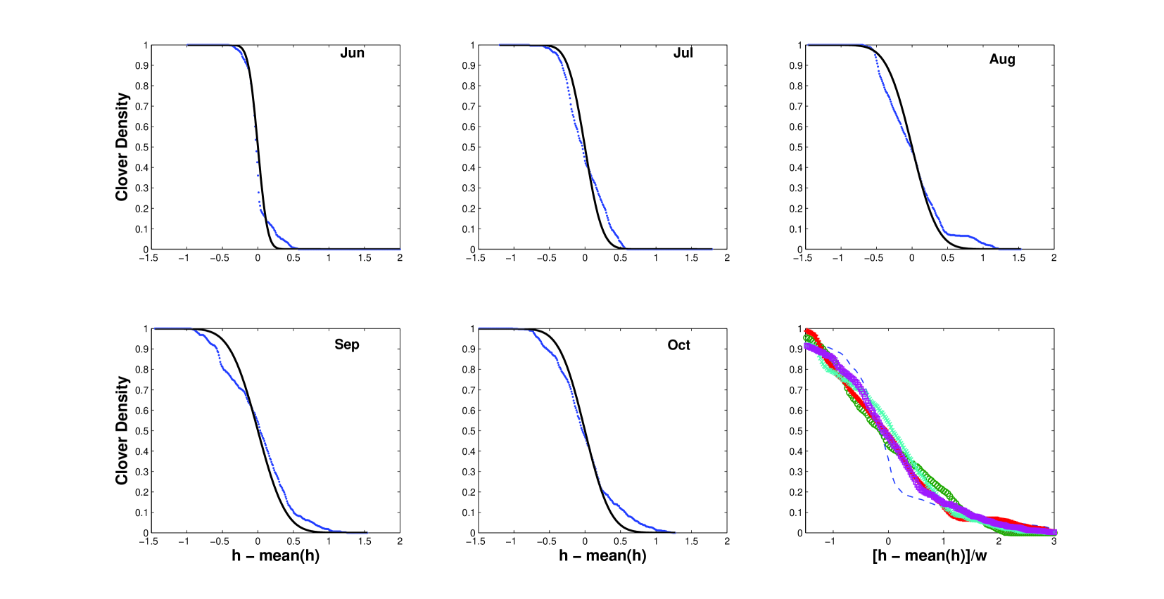
Figure 6: Density profiles of interface width, June through October (as indicated). $L=16~{}m$. Each month’s empirical profile indicated by $(\bullet)$. Associated complementary error function for each month, parameterized by observed interface width, approximates data. Interface widths for consecutive month are, respectively, $w=0.15,0.27,0.4,0.44,0.4$. Lower right. Data collapse. Dividing height (relative to front’s mean position) by interface width indicates that last four months’ clover-density profiles share structural organization. First month (broken line) insufficiently roughened to “fit.” Symbols are empty circle (Jul), square (Aug), $\times$ (Sep) and closed circle (Oct).

Figure 6 shows interface profiles from one experimental plot ($16~{}m$, same as Fig. 1) for all five months. Each profile plots the fraction of $L$ rows occupied by clover as a function of distance from that month’s mean height. Every month clover and ryegrass occurred with nearly equal frequency at the mean height. The first month’s (June) profile drops sharply; the competitors mix very little as the interface begins to develop. Closer to saturation, the profiles are less steep as interface width increases.

We can approximate observed interface profiles with the complementary error function. Let $\rho_{t}(h)$ represent clover density at height $h$ and time $t$. Then:

$$\rho_{t}(h)=\frac{1}{2}~{}erfc\left([h-\overline{h}(t)])/w_{t}\right)$$ (4)

where $w_{t}$ is interface width at time $t$. The complementary error function is:

$$erfc~{}(x)=\frac{2}{\sqrt{\pi}}\int_{x}^{\infty}exp\left[-z^{2}\right]dz$$

Equation 4 reasonably approximates observed profiles. Mean invader density has an approximately Gaussian decline across the interface; see Foltin et al [1994].

The final subplot in Fig. 6 (lower right) indicates “data collapse” of the last four months’ density profiles. Re-scaling height as $[h-\overline{h}(t)])/w_{t}$ reveals that the profiles share a common structural dependence on interface width, close to/at saturation. That is, the re-scaled plot shows the basic relationship for which the July through October profiles are examples. The first profile, a relatively un-roughened interface, has a different dependence. Interface profiles average across spatially correlated invader density, but indicate how biotic interactions are organized within the interface. Here, we neglect the density of open sites (which follows reasonably from our field results). If intraspecific interactions occur in proportion to $\left[\rho_{t}(h)\right]^{2}$, their frequency will decline faster than invader frequency within the interface. Interspecific interactions, if proportional to $\rho_{t}(h)[1-\rho_{t}(h)]$, will increase initially, peak at $\overline{h}(t)$, and then decline. Given this approximate picture, greater roughening (hence, larger width) increases interspecific mixing at the interface in a quantifiable manner; see Figure 7.

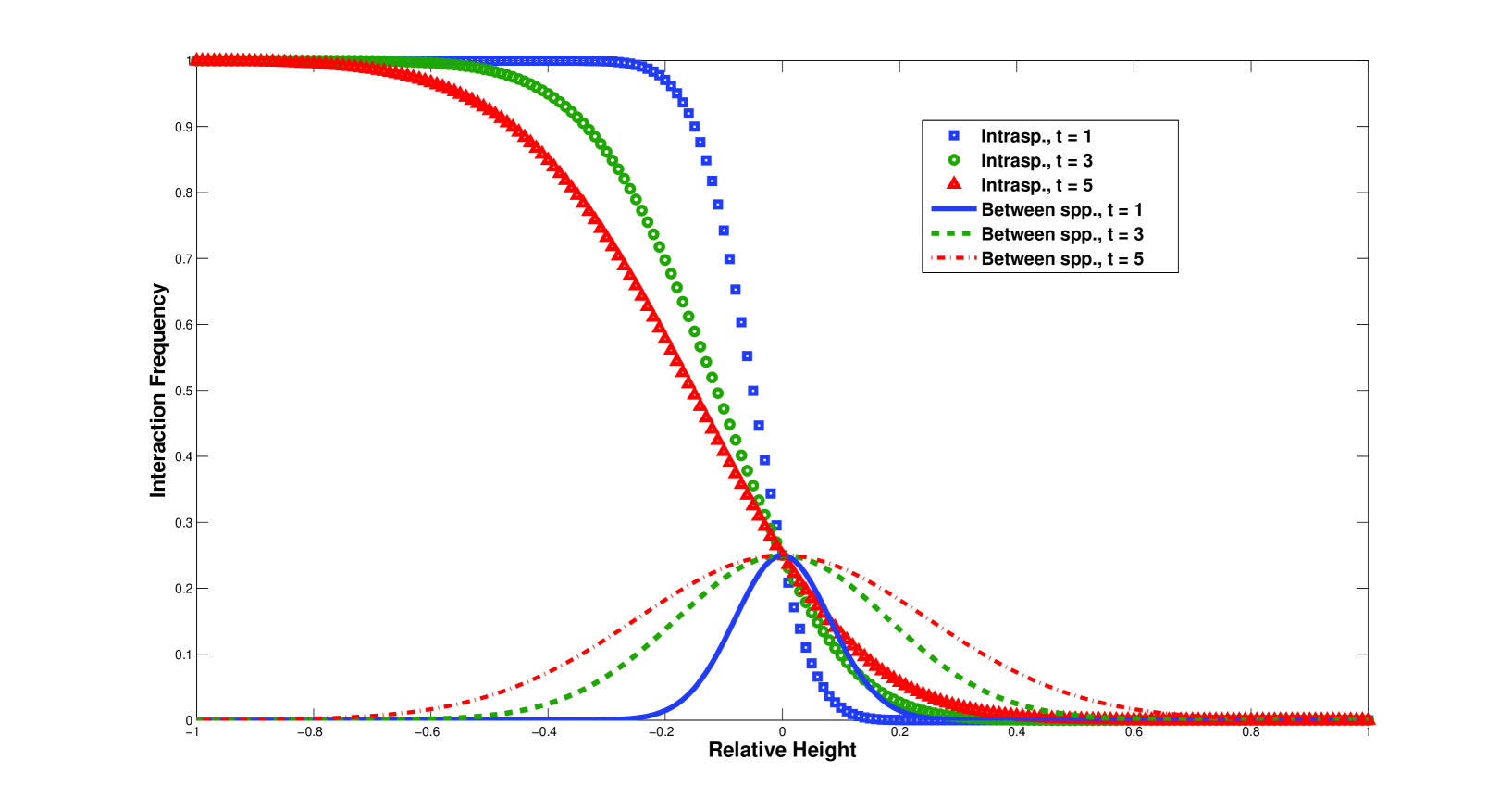
Figure 7: Invader interaction frequencies. $w(t=1)=0.13$ (blue), $w(t=3)=0.29$ (green), and $w(t=5)=0.39$ (red). As time ($t$, in months) advances, interface width increases. As width increases, (1) decline in intraspecific competition behind mean height exceeds increase in intraspecific competition in front of mean height, and (2) interspecific competition increases symmetrically about mean height.

We assumed that the interface developed from an initially linear array of individuals. But invader growth will often commence as small, nearly circular clusters of individuals. Many of the smallest clusters can disappear due to demographic stochasticity, despite an invader’s ecological superiority [Korniss and Caraco 2005]; large clusters will continue to grow. At the critical cluster size [Allstadt et al. 2007] decline and growth are equally probable. After a cluster attains sufficient size, we can treat its perimeter as a roughened “surface;” we discuss these issues in detail elsewhere [O’Malley et al. 2009a].

Our general model assumes that an invader will propagate both forward and laterally; any unoccupied, nearest-neighboring site can be colonized at the same stochastic rate. Cain et al. [1995] carefully mapped the architecture of clonal growth in a white clover population. Node-to-node branching angles of apical meristems centered on $0^{\circ}$ (straight ahead), but some large angles were observed. Lateral meristems branched off with a bimodal angular distribution, concentrated at $\pm 60-70^{\circ}$. Clover, then, exhibits both forward and lateral growth, but with an overall bias toward forward propagation. The resulting morphology could have induced the difference we observed between the scaling of the front-runner’s lead and roughening with the length of the interface.

Schwinning and Parsons [1996a,b] modeled legume-grass spatial systems, and identified conditions where a legume (e.g., clover) excludes grass competitively, where grass excludes the legume, and where the two coexist; also see Cain et al. [1995]. Low soil nitrogen (N) favors the legume; N-fixation generates a competitive advantage. Defoliation/herbivory, as opposed to its absence, can promote the legume’s competitive superiority at certain N-concentrations. High soil-N favors grass over the legume, since grass then has the greater relative growth rate [Schwinning and Parsons 1996b]. Intermediate conditions can maintain coexistence. In our field experiment, we applied just enough N-fertilizer to insure that the grass would grow sufficiently to define a clear invader-resident interface. We mowed plots periodically to prevent grass from growing tall enough to shade the clover. As a cluster of clover expands, it can increase soil-N levels. Consequently, grass may dynamically exploit the clover and compete more effectively [Schwinning and Parsons 1996b]. N-availability could have increased during the growing season; perhaps between-species competition decelerated the advance of the clover.

Cain et al. [1995] report that clover’s stolon growth self-regulates at high density. Sufficiently strong self-regulation among source ramets might reduce translocation to sink ramets, decelerating clover’s advance. However, biotic effects on velocity, in our experiment, were likely overwhelmed by seasonal change in temperature and day length.

Summarily, the theory of kinetic roughening offers a new, practical framework for understanding spatial pattern in both within and between-species interactions. Furthermore, the theory’s scaling predictions suggest a novel approach to linking local interface measures to properties of an invasive front at extended spatial scales.

ACKNOWLEDGEMENTS

We thank K. Bolton, K. Shukla, and the staff at the Guelph Turfgrass Institute and Research Station for help with the experiment. We appreciate discussion with G. Robinson, L. O’Malley, A.J. Parsons and A.C. Gorski. This material is based upon research supported by the National Science Foundation under Grant No. DEB 0918392 (TC), DEB 0918413 (GK), and DMR 1246958 (GK); field research was supported by grants from the Ontario Ministry of Agriculture (JAN) and the Canadian Natural Sciences and Engineering Research Council (JAN).

SUPPLEMENTAL MATERIAL

Appendix A Pulled versus pushed fronts

Models for spatial invasion often adopt a reaction-diffusion formalism, treating population densities as continuous variables. A deterministic reaction-diffusion system may yield an analytic approximation for invasion speed, given by the asymptotic velocity of a traveling wave [Andow et al. 1990, Caraco et al. 2002, Murray 2003]. But traveling waves invoke infinitesimal population densities [Durrett and Levin 1994, Pachepsky and Levine 2011], and the linearized front can be “pulled” by reproduction and dispersal of the invader at locations where its population density is near 0 [Lewis and Kareiva 1993, Snyder 2003]. Deterministic reaction-diffusion theory neglects the discreteness of individuals, the fundamental source of endogenous, random fluctuations, and consequently overestimates the velocity of an individual-based, dispersal-limited dynamics [Escudero et al. 2004]. Therefore, deterministic reaction-diffusion equations, and their generalizations, oversimplify the dynamics of rarity [Clark et al. 2003]; they cannot capture consequences of strong dispersal limitation, in particular, the spatially correlated variability along the interface we studied experimentally.

Discrete (individual-based) models reveal effects of nonlinear, stochastic growth processes driving an ecological interface [Wilson 1998, Moro 2001]. Discrete models predict front-propagation behaviors that differ from results of deterministic diffusion models [van Saarloos 2003]. When dispersal is limited to a local neighborhood, the interface is “pushed” at a velocity less than that of the corresponding deterministic diffusion model [Moro 2003]. As a stochastic model’s interface roughens, the distance over which density fluctuations are correlated grows [Rácz and Gálfi 1988, Majumdar and Comtet 2004]; consequently, the front-runner’s lead is an extreme value among dependent random variables.

Given the assumption that a spatially clustered invader displaces a resident competitor, the front is pushed into a meta-stable medium [Korniss and Caraco 2005]. If the same invader were to propagate into empty space (i.e., a region where the invader does not encounter biotic resistance), the front would be pushed into an unstable medium. Invasion velocity is, of course, slower in the former case [Allstadt et al. 2009]. Interestingly, the two fronts will roughen similarly; the same interface-length dependent scaling will emerge.

Appendix B Roughening and Universality

Recall the general scaling relationships of a self-affine interface [Barabási and Stanley 1995]. During development, roughness increases with time according to $\langle w^{2}(L,t)\rangle\sim t^{2\beta}$. The time of crossover to statistical equilibrium increases with interface length according to $t_{\times}\sim L^{z}$. After saturation, roughness increases with interface length according to $\langle w^{2}(L,\infty)\sim L^{2\alpha}$.

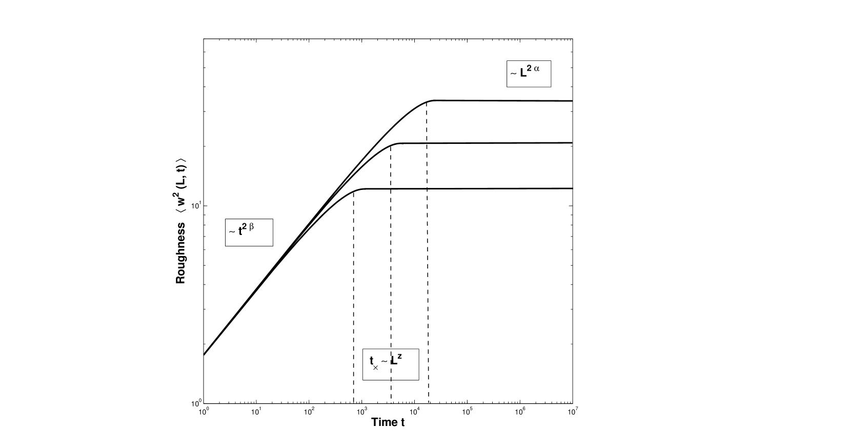
Figure 8: Roughening over time, both scaled logarithmically. $\langle w^{2}\rangle$ increases as a power law during interface development. Time of crossover and degree of roughening at saturation both scale with interface length.

Different models for individual-level demographic processes driving invasion may exhibit the same dependence of roughening on time, and the equilibrium width may exhibit the same dependence on interface length. Such roughened interfaces belong to the same “universality class;” universality offers powerful generalization. O’Malley et al. (2006) analyzed a model for an advancing front in a habitat where dispersal-limited species compete for growth sites. They found that the model’s roughening behavior belongs to the KPZ universality class, for Kardar-Parisi-Zhang [Kardar et al. 1986]. For the broad class of models exhibiting KPZ universality, roughening of a one-dimensional interface (hence the habitat has two dimensions) implies that the dynamic exponent $z$ = 3/2, the growth exponent $\beta$ = 1/3, and the roughening exponent $\alpha$ = 1/2.

Despite successful application of KPZ scaling relationships to a series of real-world questions, the model’s assumptions are fragile. The nonlinear stochastic differential equation underlying the derivation of the scaling exponents includes additive Gaussian noise, uncorrelated in space and time. If the noise, instead, has spatial or temporal power-law correlation, or if the noise remains an uncorrelated, but non-Gaussian process, then the exponents change [Sneppen 1992].

Appendix C Field Methods

Initial monocultures were established in Fall 2007, with Dutch white clover seed and a perennial ryegrass mix planted at respective densities of $>1.28$ kg/100 $m^{2}$, and $>7.5$ kg/ha. For ease of planting and establishment, plots were arranged (with one exception) so the initial monocultures of a plot border the monoculture of the same species in the next row. Experimental blocks were arranged linearly from the northeast to the southwest. Spatial constraints required two rows within each block, aligned from the northwest to the southeast. One row in each block contained plots of $L$ = 1 and 16 $m$ side by side, separated by their buffer areas, plus an additional one meter gap to ensure independence of the plots. The other row contained plots of the remaining $L$ in the same manner. The order of the rows within the block and the position of plots within a row were randomly selected. Blocking exerted no significant statistical effects on the results.

The ryegrass mix consisted of 40% Barclay, 30% Passport, and 30% Goalkeeper varieties. The area was watered as necessary, and the well drained, sandy loam soil prevented excessive moisture accumulation. The ryegrass required fertilization twice before it became fully established (on 7/7/2008 and 9/19/2008; each time we applied 25kgN/ha). To remove weeds without disturbing the soil, we sprayed herbicide twice (7/7/2008 and 9/19/08). The clover was sprayed with a grass control herbicide (Poast Ultra, 1L/ha), and the grass with a broad-leaf control herbicide (Par 3, 55mL/100$m^{2}$). Throughout the experiment, we removed weeds manually, unless removal would disturb the interface.

In spring 2009, monocultures achieved densities sufficient for the experiment. On May 20th, plastic barriers between monocultures were removed. Plots were mowed weekly to 5 $cm$ above ground through the end of October 2009. There was very little advance of the front in this first season (no movement in most plots) possibly due to the intense mowing regime. In 2010, we mowed only once a month to 8 $cm$ above ground, and the clover steadily advanced. We took monthly photos just after mowing. Throughout the experiment, weeds surviving mowing were manually removed, provided their removal did not disturb the advancing interface.

References

- [Allstadt et al. 2007] Allstadt, A., T. Caraco, and G. Korniss. 2007. Ecological invasion: spatial clustering and the critical radius. Evolutionary Ecology Research 9:375–394.
- [Allstadt et al. 2009] Allstadt, A., T. Caraco, and G. Korniss. 2009. Preemptive spatial competition under a reproduction-mortality constraint. Journal of Theoretical Biology 258:537–549.
- [Allstadt et al. 2012] Allstadt, A., T. Caraco, F. Molnar, Jr., and G. Korniss. 2012. Interference competition and invasion: spatial structure, novel weapons, and resistance zones. Journal of Theoretical Biology 306:46–60.
- [Andow et al. 1990] Andow, D.A., P.M. Kareiva, S.A. Levin, and A. Okubo. 1990. Spread of invading organisms. Landscape Ecology 4:177–188.
- [Antonovics et al. 2006] Antonovics, J., A.J. McKane, and T.J. Newman. 2006. Spatiotemporal dynamics in marginal populations. American Naturalist 167:16–27.
- [Barabási and Stanley 1995] Barabási, A.-L., and H.E. Stanley. 1995. Fractal concepts in surface growth. Cambridge (UK): Cambridge University Press. 386 p.
- [Brú et al. 2003] Brú, A., S. Albertos, J. L. Subiza, J. L. García-Asenjo, and I. Brú. 2003. The universal dynamics of tumor growth. Biophysics Journal 85:2948–2961.
- [Burnham and Anderson 2002] Burnham, K.P., and D.R. Anderson. 2002. Model selection and multimodel inference: a practical information-theoretic approach. Springer Verlag, Heidelberg DE.
- [Cain et al. 1995] Cain, M.L., S.W. Pacala, J.A. Silander Jr., and M.-J. Fortin. 1995. Neighborhood models of clonal growth in the white clover Trifolium repens. American Naturalist 145:888–917.
- [Cantor et al. 2011] Cantor, A., A. Hale, J. Aaron, M.B. Traw, and S. Kalisz. 2011. Low allelochemical concentrations detected in garlic mustard-invaded forest soils inhibit fungal growth and AMF spore germination. Biological Invasions 13, 3015–3025.
- [Caraco et al. 2002] Caraco, T., S. Glavanakov, G. Chen, J.E. Flaherty, T.K. Ohsumi, and B.K. Szymanski. 2002. Stage-structured infection transmission and a spatial epidemic: a model for Lyme disease. American Naturalist 160:348–359.
- [Chesson 2000] Chesson, P. 2000. Mechanisms of maintenance of species diversity. Annual Review of Ecology and Systematics 31:343–366.
- [Clark et al. 2001] Clark, J.S., M. Lewis, and L. Horvath. 2001. Invasion by extremes: population spread with variation in dispersal and reproduction. American Naturalist 157:537–554.
- [Clark et al. 2003] Clark, J.S., M. Lewis, J.S. McLachlan, and J. HilleRisLambers. 2003. Estimating population spread: what can we forecast and how well? Ecology 84:1979–1988.
- [Condit et al. 2000] Condit, R., P.S. Ashton, P. Baker, S. Bunyavejchewin, S. Gunatilleke, et al. 2000. Spatial patterns in the distribution of tropical tree species. Science 288:1414–1418.
- [Dale 1999] Dale, M.R.T. 1999. Spatial pattern analysis in plant ecology. Cambridge University Press, Cambridge, UK
- [Durrett and Levin 1994] Durrett, R., and S.A. Levin. 1994. The importance of being discrete (and spatial). Theoretical Population Biology 46:363–394.
- [Duryea et al. 1999] Duryea, M., T. Caraco, G. Gardner, W. Maniatty, and B.K. Szymanski. 1999. Population dispersion and equilibrium infection frequency in a spatial epidemic. Physica D 132:511–519.
- [Eppinga et al. 2013] Eppinga, M.B., C.A. Pucko, M. Baudena, B. Beckage, and J. Molofsky. 2013. A new method to infer vegetation boundary movement from ‘snapshot’ data. Ecography 36:622–625.
- [Escudero et al. 2004] Escudero, C., J. Buceta, F.J. de la Rubia, and K. Lindenberg. 2004. Extinction in population dynamics. Physical Review E 69:021908, 9 p.
- [Family and Vicsek 1985] Family, F., and T. Vicsek. 1985. Scaling of the active zone in the Eden process on percolation networks and the ballistic deposition model. Journal of Physics A 18:L75 -L81.
- [Fisher and Tippett 1928] Fisher, R.A., and L.H.C. Tippett. 1928. The frequency distribution of the largest or smallest member of a sample. Proceedings of the Cambridge Philosophical Society 24:180–191.
- [Foltin et al. 1994] Foltin, G., K. Oerding, Z. Rácz, R.L. Workman, R.K.P. Zia. 1994. Width distribution for random-walk interfaces. Physical Reviews E 50:R639–R642.
- [Fraser 1989] Fraser, J. 1989. Characteristics of naturalized populations of white clover (Trifolium repens) in Atlantic Canada. Canadian Journal of Botany 67:2297–2301.
- [Fustec et al. 2005] Fustec, J., J. Guilleux, J. Le Corff, and J.P. Maitre. 2005. Comparison of early development of three grasses: Lolium perenne, Agrostis stolonifera and Poa pratensis. Annals of Botany 96:269–278.
- [Galambos et al. 1994] Galambos, J., J. Lechner, and E. Simin (Eds). 1994. Extreme value theory and applications. Kluwer, Dordrecht.
- [Galeano et al. 2003] Galeano, J., J. Buceta, K. Juarez, B. Pumarino, J. de la Torre, and J.M. Iriondo. 2003. Dynamical scaling analysis of plant callus growth. Europhysics Letters 63:83–89.
- [Gandhi et al. 1999] Gandhi, A., S. Levin, and S. Orszag. 1999. Nucleation and relaxation from meta-stability in spatial ecological models. Journal of Theoretical Biology 200:1221–146.
- [Gastner et al. 2009] Gastner, M.T., B. Oborny, D.K. Zimmermann, and G. Pruessner. 2009. Transition from connected to fragmented vegetation across an environmental gradient: scaling laws in ecotone geometry. American Naturalist 174:E23–E39.
- [Goldberg and Barton 1992] Goldberg, D.E., and A.M. Barton. 1992. Patterns and consequences of interpsecific competition in natural communities: a review of field experiments with plants. American Naturalist 139:771–801.
- [Gough et al. 2002] Gough, L., D.E. Goldberg, C. Hershock, N. Pauliukonis, and M. Petru. 2002. Investigating the community consequences of competition among clonal plants. Evolutionary Ecology 15:547–563.
- [Hajek et al. 1996] Hajek, A.E., J.S. Elkinton, and J.J. Witcosky. 1996. Introduction and spread of the fungal pathogen Entomophaga maimaiga (Zygomycetes:Entomophthorales) along the leading edge of Gypsy Moth (Lepidoptera:Lymantriidae) spread. Environmental Entomology 25:1225–1247.
- [Harada and Iwasa 1994] Harada, Y., and Y. Iwasa. 1994. Lattice population dynamics for plants with dispersing seeds and vegetative propagation. Researches on Population Ecology 36:237–249.
- [Herben et al. 2000] Herben, T., H.J. During, and R. Law. 2000. Spatio-temporal patterns in grassland communities. In The geometry of ecological interactions, U. Dieckmann, R. Law, and J.A.J. Metz (Eds.), pp. 48–64. Cambridge University Press, Cambridge UK.
- [Karabacak et al. 2001] Karabacak, T., Y.-P. Zhao, G.-C. Wang, and T.-M. Lu. 2001. Growth-front roughening in amorphous silicon films by sputtering. Physical Review B 64:085323 (10 pp).
- [Kardar et al. 1986] Kardar, M., G. Parisi, and Y.-C. Zhang. 1986. Dynamic scaling of growing interfaces. Physical Review Letters 56:889–892.
- [Kolar and Lodge 2001] Kolar, C.S., and D.M. Lodge. 2001. Progress in invasion biology: predicting invaders. Trends in Ecology & Evolution 16:199–204.
- [Korniss and Caraco 2005] Korniss, G., and T. Caraco. 2005. Spatial dynamics of invasion: the geometry of introduced species. Journal of Theoretical Biology 233:137–150.
- [Korniss et al. 2000] Korniss, G., Z. Toroczkai, M. A. Novotny, and P. A. Rikvold. 2000. From massively parallel algorithms and fluctuating time horizons to nonequilibrium surface growth. Physical Review Letters 84:1351–1354.
- [Korniss et al. 2003] Korniss, G., M. A. Novotny, H. Guclu, Z. Toroczkai, and P. A. Rikvold. 2003. Suppressing roughness of virtual times in parallel discrete-event simulations. Science 299:677–679.
- [Krug and Meakin 1990] Krug, J., and P. Meakin. 1990. Universal finite-size effects in the rate of growth processes. Journal of Physics A 23:L987, 9 p.
- [Kui et al. 2013] Kui, L., F. Li, G. Moore, and J. West. 2013. Can the riparian invader, Arundo donax, benefit from clonal integration? Weed Research 53:370–377.
- [Levine et al. 2004] Levine, J.M., Adler, P.B., Yelenik, S.G. 2004. A meta-analysis of biotic resistance to exotic plant invasions. Ecology Letters 7:975–989.
- [Lewis and Kareiva 1993] Lewis, M.A., and P. Kareiva. 1993. Allee dynamics and the spread of invading organisms. Theoretical Population Biology 43:141–158.
- [Liu et al. 2006] Liu, J., M. Dong, S.L. Miao, Z.Y. Li, M.H. Song, and R.Q. Wang. 2006. Invasive alien plants in China: role of clonality and geographical origin. Biological Invasions 8:1461–1470.
- [Majumdar and Comtet 2004] Majumdar, S.N., and A. Comtet. 2004. Exact maximal height distribution of fluctuation interfaces. Physical Review Letters 92:225501, 4 p.
- [Majumdar and Comtet 2005] Majumdar, S.N., and A. Comtet. 2005. Airy distribution function: from the area under a Brownian excursion to the maximal height of fluctuating interfaces. Journal of Statistical Physics 119:776–826.
- [Moro 2001] Moro, E. 2001. Internal fluctuations effects on Fisher waves. Physical Review Letters 87:238303, 4 p.
- [Moro 2003] Moro, E. 2003. Emergence of pulled fronts in fermionic microscopic particle models. Physical Review E 68:025102, 4 p.
- [Murray 2003] Murray, J.D. 2003. Mathematical biology, Vol 2. Springer, New York.
- [O’Malley et al. 2006] O’Malley, L., B. Kozma, G. Korniss, Z. Rácz, and T. Caraco. 2006. Fisher waves and front propagation in a two-species invasion model with preemptive competition. Physical Reviews E 74:041116, 7 p.
- [O’Malley et al. 2009a] O’Malley, L., G. Korniss, and T. Caraco. 2009. Ecological invasion, roughened fronts, and a competitor’s extreme advance: integrating stochastic spatial-growth models. Bulletin of Mathematical Biology 71:1160–1188.
- [O’Malley et al. 2009b] O’Malley, L., B. Kozma, G. Korniss, Z. Rácz, and T. Caraco. 2009. Fisher waves and the velocity of front propagation in a two-species invasion model with preemptive competition. In Computer Simulation Studies in Condensed Matter Physics XIX, D. P. Landau, S. P. Lewis, and H.-B. Schüttler (Eds.), Springer proceedings in physics Vol. 123, pp. 73-78. Springer, Heidelberg.
- [O’Malley et al. 2010] O’Malley, L., G. Korniss, S.S.P. Mungara, and T. Caraco. 2010. Spatial competition and the dynamics of rarity in a temporally varying environment. Evolutionary Ecology Research 12:279–305.
- [Pachepsky and Levine 2011] Pachepsky, E., and J.M. Levine. 2011. Density dependence slows invader spread in fragmented landscapes. American Naturalist 177:18–28.
- [Pechenik and Levine 1999] Pechenik, L., and H. Levine. 1999. Interfacial velocity corrections due to multiplicative noise. Physical Review E 59:3893–3900.
- [Plischke et al. 1987] Plischke, M., Z. Rácz, and D. Liu. 1987. Time-reversal invariance and universality of two-dimensional models. Physical Review B:3485–3495.
- [Rácz and Gálfi 1988] Rácz, Z., and L. Gálfi. 1988. Properties of the reaction front in an A + B C type reaction-diffusion process. Physical Review A 38:3151–3154.
- [Sakai et al. 2001] Sakai, A.K., F.W. Allendorf, J.S. Holt, D.M. Lodge, J. Molofsky, K.A. With, S. Baughman, R.J. Cabin, J.E. Cohen, N.C. Ellstrand, D.E. McCauley, P. O’Neil, I.M. Parker, J.N. Thompson, and S.G. Weller. 2001. The population biology of invasive species. Annual Review of Ecology and Systematics 32:305–332.
- [Schehr and Majumdar 2006] Schehr, G., and S.N. Majumdar. 2006. Universal asymptotic statistics of a maximal relative height in one-dimensional solid-on-solid models. Physical Review E 73:056103, 10 p.