The strongest gravitational lenses: III. The order statistics of the largest Einstein radii

Abstract

Context. The Einstein radius of a gravitational lens is a key characteristic. It encodes information about decisive quantities such as halo mass, concentration, triaxiality, and orientation with respect to the observer. Therefore, the largest Einstein radii can potentially be utilised to test the predictions of the $\Lambda$CDM model.

Aims. Hitherto, studies have focussed on the single largest observed Einstein radius. We extend those studies by employing order statistics to formulate exclusion criteria based on the $n$ largest Einstein radii and apply these criteria to the strong lensing analysis of 12 MACS clusters at $z>0.5$.

Methods. We obtain the order statistics of Einstein radii by a Monte Carlo approach, based on the semi-analytic modelling of the halo population on the past lightcone. After sampling the order statistics, we fit a general extreme value distribution to the first-order distribution, which allows us to derive analytic relations for the order statistics of the Einstein radii.

Results. We find that the Einstein radii of the 12 MACS clusters are not in conflict with the $\Lambda$CDM expectations. Our exclusion criteria indicate that, in order to exhibit tension with the concordance model, one would need to observe approximately twenty Einstein radii with $\theta_{\rm eff}\gtrsim 30\arcsec$, ten with $\theta_{\rm eff}\gtrsim 35\arcsec$, five with $\theta_{\rm eff}\gtrsim 42\arcsec$, or one with $\theta_{\rm eff}\gtrsim 74\arcsec$ in the redshift range $0.5\leq z\leq 1.0$ on the full sky (assuming a source redshift of $z_{\rm s}=2$). Furthermore, we find that, with increasing order, the haloes with the largest Einstein radii are on average less aligned along the line-of-sight and less triaxial. In general, the cumulative distribution functions steepen for higher orders, giving them better constraining power.

Conclusions. A framework that allows the individual and joint order distributions of the $n$-largest Einstein radii to be derived is presented. From a statistical point of view, we do not see any evidence of an Einstein ring problem even for the largest Einstein radii of the studied MACS sample. This conclusion is consolidated by the large uncertainties that enter the lens modelling and to which the largest Einstein radii are particularly sensitive.

1 Introduction

The Einstein radius (Einstein 1936), suitably generalised to non-circular lenses, is a key characteristic of every strong lensing system (see e.g. Bartelmann 2010; Kneib & Natarajan 2011; Meneghetti et al. 2013, for recent reviews of gravitational lensing). As a measure of the size of the tangential critical curve, it is very sensitive to a number of basic halo properties, such as the density profile, concentration, triaxiality, and the alignment of the halo with respect to the observer, but also to the lensing geometry, which is fixed by the redshifts of the lens and the sources (see e.g. Oguri et al. 2003; Oguri & Blandford 2009). Moreover, the distribution of the sample of Einstein radii as a whole is strongly influenced by the underlying cosmological model. Here, not only cosmological parameters like the matter density, $\Omega_{\rm m}$, and the amplitude of the mass fluctuations, $\sigma_{8}$, but also the choice of the mass function, as well as the merger rate, have a strong impact.

Recent studies gave rise to the so-called Einstein ring problem, the claim that the largest observed Einstein radii (see e.g. Halkola et al. 2008; Umetsu & Broadhurst 2008; Zitrin et al. 2011, 2012) exceed the expectations of the standard $\Lambda$CDM cosmology (Broadhurst & Barkana 2008; Oguri & Blandford 2009; Meneghetti et al. 2011). The comparison of theory and observations was performed by either comparing the largest observed Einstein radii with semi-analytic estimates of the occurrence probabilities of the strongest observed lens systems or with those found in numerical simulations. The most realistic treatment is certainly based on numerical simulations, which naturally include the impact of gas physics and mergers. However, for the statistical assessment of the strongest gravitational lenses, the number of simulation boxes and their sizes themselves are usually too small to sufficiently sample the extreme tail of the Einstein ring distribution. A sufficient sampling of the extreme value distribution of the largest Einstein radius roughly requires the simulation of $\sim 1000$ mock universes and a subsequent strong lensing analysis for each cluster sized halo (Waizmann et al. 2012).

In this series of papers on the strongest gravitational lenses, we studied several aspects of the Einstein radius distribution. We utilised a semi-analytic approach that allows a sufficient sampling of the extreme tail of the Einstein radius distribution at the cost of a simplified lens modelling. In the first paper (Redlich et al. 2012, herafter Paper I), we introduced our method for the semi-analytic modelling of the Einstein radius distribution. We then studied the impact of cluster mergers on the optical depth for giant gravitational arcs of selected cluster samples and on the distribution of the largest Einstein radii. The second work (Waizmann et al. 2012, herafter Paper II) focussed on the extreme value distribution of the Einstein radii and the effects that strongly affect it, such as triaxiality, alignment, halo concentration, and the mass function. We could also show that the largest known observed Einstein radius at redshifts of $z>0.5$ of MACS J0717.5+3745 (Zitrin et al. 2009a, 2011; Medezinski et al. 2013) is consistent with the $\Lambda$CDM expectations. Now, in the third paper of this series, we extend the previous works by applying order statistics to the distribution of Einstein radii. Inference based on a single observation is difficult for it is a priori unknown whether the maximum is really drawn from the supposedly underlying distribution, or whether it is an event caused by a very peculiar situation that was statistically not accounted for. This is particularly important for strong lensing systems, which are heavily influenced by a number of different physical effects. It is therefore desirable to formulate $\Lambda$CDM exclusion criteria that are based on a number of observations instead of a single event. This goal can be accomplished by means of order statistics. We obtain the order statistic by Monte Carlo (MC) sampling of the hierarchy of the largest Einstein radii, using the semi-analytic method from Paper I, which is based on the work of Jing & Suto (2002); Oguri et al. (2003), and Oguri & Blandford (2009). By fitting the generalised extreme value distribution to the first-order distribution, we derive analytic expressions for all order distributions and use them to formulate $\Lambda$CDM exclusion criteria. In the last part, we finally compare the theoretical distributions with the results of the strong lensing analysis of 12 clusters of the massive cluster survey (MACS, Ebeling et al. 2001, 2007) at redshifts of $z>0.5$ by Zitrin et al. (2011).

This paper is structured as follows. In Sect. 2, we introduce the mathematical prerequisites of order statistics, followed by a brief summary of the method for semi-analytically modelling the distribution of Einstein radii in Sect. 3. Then, in Sect. 4, we present first results of the MC sampling of the order statistics. Afterwards, in Sect. 5.1, we study the order statistical distributions and derive exclusion criteria based on the $n$ largest Einstein radii. This is followed by a comparison with the MACS sample in Sect. 5.2 and an introduction of the joint two-order distributions in Sect. 5.3. In Sect. 6, we briefly summarize our main results and finally conclude.

For consistency with our previous studies, we adopt the Wilkinson Microwave Anisotropy Probe 7–year (WMAP7) parameters $(\Omega_{\Lambda 0},\Omega_{{\rm m}0},\Omega_{{\rm b}0},h,\sigma_{8})=(0.727,0.273,0.0455,0.704,0.811)$ (Komatsu et al. 2011) throughout this work.

2 Order statistics

In this section, we briefly summarise the mathematical prerequisites of order statistics that are needed for the remainder of this work. A more thorough treatment can be found in the excellent textbooks of Arnold et al. (1992) and David & Nagaraja (2003) or, in a cosmological context, in Waizmann et al. (2013).

Suppose that $X_{1},X_{2},\dots,X_{n}$ is a random sample of a continuous population with the probability density function (pdf) $f(x)$ and the corresponding cumulative distribution function (cdf) $F(x)$. Then, the order statistic is given by the random variates ordered by magnitude $X_{(1)}\leq X_{(2)}\leq\cdots\leq X_{(n)}$, where $X_{(1)}$ is the smallest (minimum) and $X_{(n)}$ denotes the largest (maximum) variate in the sample. The pdf of $X_{(i)}\,(1\leq i\leq n)$ of the $i$-th order is then found to be given by

$$f_{(i)}(x)=\frac{n!}{(i-1)!(n-i)!}\left[F(x)\right]^{i-1}\left[1-F(x)\right]^{n-i}f(x)\,.$$ (1)

Correspondingly, the cdf of the $i$-th order is given by

$$F_{(i)}(x)=\sum_{k=i}^{n}\binom{n}{k}\left[F(x)\right]^{k}\left[1-F(x)\right]^{n-k}\,.$$ (2)

The distribution functions of the special cases of the lowest and the highest values are then readily found to be

$$F_{(1)}(x)=1-\left[1-F(x)\right]^{n}$$ (3)

and

$$F_{(n)}(x)=\left[F(x)\right]^{n}\,.$$ (4)

For large sample sizes, both $F_{(n)}(x)$ and $F_{(1)}(x)$ can be described by a member of the general extreme value (GEV) distribution (Fisher & Tippett 1928; Gnedenko 1943) as used in Paper II of this series. In this case, the cdf is given by

$$G(x)=\exp{\left\{-\left[1+\gamma\left(\frac{x-\alpha}{\beta}\right)\right]^{-1/\gamma}\right\}}\,,$$ (5)

where $\alpha$, $\beta$, and $\gamma$ are respectively the location-, scale-, and shape-parameter, which can either be obtained directly from the data or from an underlying model assumption (see Coles (2001), for instance).

The distribution functions of the single-order statistics can be generalised to $n$-dimensional joint distributions. In this work, we do not go beyond the two-order statistics for which the joint pdf $X_{(r)},X_{(s)}\;(1\leq r<s\leq n)$ for $x<y$ reads as

$$f_{(r)(s)}(x,y)= \frac{n!}{(r-1)!(s-r-1)!(n-s)!}$$

$$\times\left[F(x)\right]^{r-1}\left[F(y)-F(x)\right]^{s-r-1}\left[1-F(y)\right]^{n-s}$$

$$\times f(x)f(y)\,.$$ (6)

The joint cumulative distribution function can be derived by directly integrating the above pdf or by a direct argument, and is given by

$$F_{(r)(s)}(x,y)= \sum_{j=s}^{n}\sum_{i=r}^{j}\frac{n!}{i!(j-i)!(n-j)!}$$

$$\times\,\left[F(x)\right]^{i}\left[F(y)-F(x)\right]^{j-i}\left[1-F(y)\right]^{n-j}\,.$$ (7)

We refer the interested reader to Appendix A of Waizmann et al. (2013) for more details on the implementation of the order statistics.

3 Semi-analytic modelling of the distribution of Einstein radii

The adopted method for the semi-analytic modelling of the distribution of Einstein radii has already been thoroughly presented in two previous papers of this series (see Redlich et al. 2012; Waizmann et al. 2012, and references therein). Thus, we only repeat the most important definitions and relations that are needed to follow this work.

3.1 Defining the Einstein radius

Historically, the Einstein radius has been defined for axially symmetric lenses. This assumption is untenable for realistic lenses, which exhibit irregular tangential critical curves. One generalised definition of the Einstein radius for arbitrarily shaped lenses is the effective Einstein radius, $\theta_{\rm eff}$, which is defined as

$$\theta_{\rm eff}\equiv\sqrt{\frac{A}{\pi}}\;,$$ (8)

where $A$ is the area enclosed by the critical curve. In the rest of this work, we only consider the effective Einstein radius.

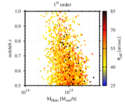
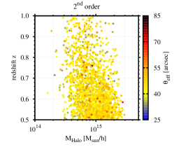
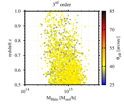
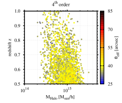
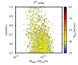
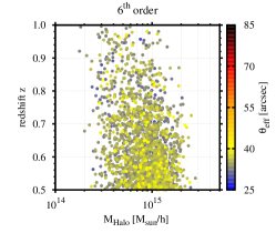
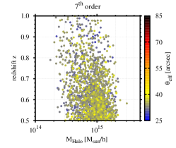
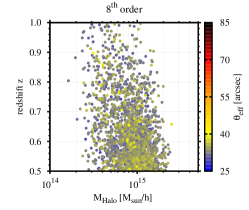
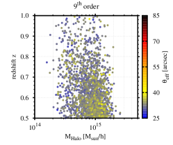
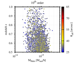
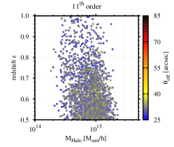
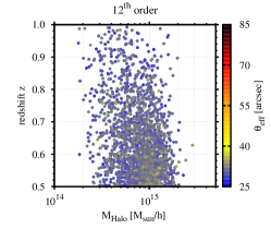
Figure 1: Distribution in mass and redshift of $2\,000$ sampled values of the effective Einstein radius of the twelve largest orders as indicated above each panel. We assume the redshift interval of $0.5\leq z\leq 1.0$ on the full sky, the Tinker et al. (2008) mass function, and a source redshift of $z_{\rm s}=2.0$. The colour encodes the size of the individual effective Einstein radii of a given order from each simulation run.

3.2 Modelling triaxial haloes

Any realistic modelling of the distribution of Einstein radii has to account for halo triaxiality. An integral part of including triaxiality in the semi- analytic modelling is the probability density functions of the axis ratios as they have been empirically derived by Jing & Suto (2002). Assuming the ordering $\left(a\leq b\leq c\right)$ of the axes, they read as

$$p(a/c) =\frac{1}{\sqrt{2\pi}\sigma_{s}}\exp\left[-\frac{(a_{\mathrm{sc}}-0.54)^{2}}{2\sigma_{\mathrm{s}}^{2}}\right]\frac{\mathrm{d}a_{\mathrm{sc}}}{\mathrm{d}(a/c)}\;,$$ (9)

$$p(a/b|a/c) =\dfrac{3}{2(1-r_{\mathrm{min}})}\left[1-\left(\dfrac{2a/b-1-r_{\mathrm{min}}}{1-r_{\mathrm{min}}}\right)^{2}\right]\;,$$ (10)

where

$$a_{\mathrm{sc}}=\frac{a}{c}\left(\frac{M}{M_{*}}\right)^{0.07[\Omega_{{\rm m}}(z)]^{0.7}}\;,\quad r_{\mathrm{min}}=\operatorname{max}\left(a/c,0.5\right)\;.$$ (11)

Equation (10) holds for $a/b\geq r_{\mathrm{min}}$ and is zero otherwise. $M_{*}$ is the characteristic non-linear mass scale. For the width $\sigma_{\rm s}$ of the axis-ratio distribution $p(a/c)$, we adopt the value $\sigma_{\rm s}=0.113$ as reported in Jing & Suto (2002).

In addition to the halo-triaxiality, the concentration parameter $c_{\rm e}$ plays an important role in defining a lensing system. The concentration is defined as $c_{\rm e}\equiv R_{\rm e}/R_{0}$, where $R_{\rm e}$ is chosen such that the mean density within the ellipsoid of the major axis radius $R_{\rm e}$ is $\Delta_{\rm e}\Omega(z)\rho_{\rm crit}(z)$, with

$$\Delta_{\rm e}=5\Delta_{\rm vir}(z)\left(c^{2}/ab\right)^{0.75}.$$ (12)

The virial overdensity, $\Delta_{\rm vir}(z)$, is approximated according to Nakamura & Suto (1997). For the pdf of the concentration parameter, Jing & Suto (2002) find the log-normal distribution

$$p(c_{\rm e})=\frac{1}{\sqrt{2\pi}\sigma_{\rm c}}\exp\left[-\frac{(\ln c_{\rm e}-\ln\bar{c}_{\rm e})^{2}}{2\sigma_{\rm c}^{2}}\right]\frac{1}{c_{\rm e}},$$ (13)

with a dispersion of $\sigma_{\rm c}=0.3$. The correlation between the axis ratio $a/c$ and the mean concentration can be modelled by the following relation (Oguri et al. 2003)

$$\bar{c}_{\mathrm{e}} =f_{\rm c}A_{\rm e}\sqrt{\frac{\Delta_{\mathrm{vir}}(z_{\rm c})}{\Delta_{\mathrm{vir}}(z)}}\left(\frac{1+z_{\rm c}}{1+z}\right)^{3/2}\;,$$ (14)

$$f_{\rm c} =\mathrm{max}\left\{0.3,1.35\exp\left[-\left(\frac{0.3}{a_{\mathrm{sc}}}\right)^{2}\right]\right\}\;,$$ (15)

where $z_{\rm c}$ is the collapse redshift. The prefactor $f_{\rm c}$, defined in Eq. 15, is a correction introduced by Oguri & Blandford (2009) in order to avoid unrealistically low concentrations for particularly small axis ratios $a_{\rm sc}$. Following Jing & Suto (2002), the free parameter $A_{\rm e}$ is set to a value of $A_{\rm e}=1.1$. All expressions listed so far are valid for the standard $\Lambda$CDM model and an inner slope of the density profile of $\alpha_{\rm NFW}=1.0$. As discussed in the previous works of this series, we force all sampled axis ratios $a_{\mathrm{sc}}$ to lie within the range of two standard deviations. By doing so, we avoid unrealistic scenarios with extremely small axis ratios and correspondingly low concentrations, where the lensing potential is dominated by masses well outside the virial radius.

A more detailed discussion of the semi-analytic modelling can be found in Jing & Suto (2002), Oguri et al. (2003), and in the previous works of this series.

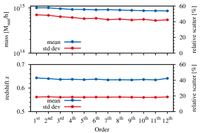
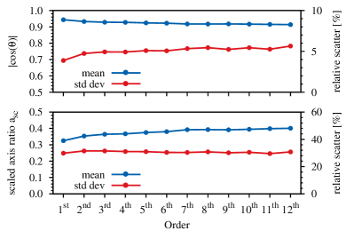
Figure 2: Dependence of the sample mean (blue lines) and relative scatter (red lines) on the chosen order for the halo mass (upper left-hand panel), the redshift (lower left-hand panel), the alignment $|\cos(\theta)|$ (upper right-hand panel), and the scaled axis ratio, $a_{\rm sc}$ (lower right-hand panel). The red arrows denote constant shifts in the standard deviation in order to enhance the readability. The results are based on the samples presented in Fig. 1, comprising $2\,000$ sampled values in the redshift range of $0.5\leq z\leq 1.0$ on the full sky.

4 Results of the MC sampling of the order statistics

The approach for sampling the order statistics of the Einstein radii is identical to the one used in Paper II. We create a large number of mock realisations of the cluster population on the past null cone, compute their strong lensing characteristics, and collect the Einstein radii of the largest orders. In this work, we use the Tinker et al. (2008) mass function for all calculations. Because we eventually intend to compare our sampled distributions with the observed sample of $12$ MACS clusters in the interval $0.5\leq z\leq 0.6$, we only consider clusters in the redshift range $0.5\leq z\leq 1$ for our study of the order statistics of Einstein radii. This choice of the redshift interval also drastically reduces the number of haloes that have to be simulated. To mimic the strong lensing analysis by Zitrin et al. (2011), we furthermore assume a fixed source redshift of $z_{\rm s}=2.0$.

In Paper II, we showed that $\leavevmode\nobreak\ 1000-2000$ realisations are sufficient for sampling the cdf of the largest Einstein radii and that all maxima stem from masses $M>2\times 10^{14}\,M_{\odot}/h$. While the first statement will certainly hold for the order statistics, the second might not be valid any more for distributions of higher orders of the Einstein radius. To verify the second assumption, we decided to sample $2000$ mock realisations, adopting a lower mass limit of $M_{\rm lim}=10^{14}\,M_{\odot}/h$. The distribution in mass and redshift for the first twelve orders is shown by Fig. 1. It clearly demonstrates that, for the higher orders, only a few values fall below the previous limit of $M>2\times 10^{14}\,M_{\odot}/h$. We will thus adopt the more conservative lower mass limit of $M_{\rm lim}=10^{14}\,M_{\odot}/h$ for the rest of this work.

Furthermore, the distributions indicate that all orders stem from a wide range of masses. This tendency is confirmed by Fig. 2, which shows the dependence of the sample mean and the relative scatter in mass and redshift for the first twelve orders. It can be seen that the sample mean in mass (upper left-hand panel) weakly drops with increasing order and exhibits a large relative scatter of $\sim 40$ per cent. Although, on average, the sample of the largest Einstein radii stems from massive clusters with $M\sim 10^{15}\,M_{\odot}$, the large scatter indicates that it is not unlikely for notably less massive clusters to contribute to this ordered list of very large Einstein radii. The sample mean of the clusters’ redshifts (lower left-hand panel) is independent of the order and shows a relative scatter of $\sim 20$ per cent. This is because the distribution in redshift is mainly determined by the lensing geometry, which is obviously independent of the considered order.

In addition to the mass and redshift distributions, it is interesting to examine how the orientation of the haloes and their scaled axis ratios depend on the different orders. For this purpose, we also calculated the sample mean and the relative scatter of the alignment, $|\cos(\theta)|$, and the scaled axis ratio, $a_{\rm sc}$, and present them in the right-hand panel of Fig. 2. A value of $|\cos(\theta)|=1$ corresponds to a perfect alignment of the halo’s major axis with the line-of-sight of the observer. It can be seen (upper panel) that the mean alignment for the first twelve orders is high $(>0.9)$, but slightly decreases with increasing order. Thus, the higher the order, the more likely it happens that the haloes are no longer perfectly aligned with the observer’s line-of-sight. This result can be easily understood. For the very largest Einstein radii, all parameters (mass, orientation, concentration, etc.) simultaneously need to be most beneficial (in terms of strong lensing efficiency). For higher orders, a slightly disadvantageous setting of one parameter (e.g. a slightly misaligned halo) can still be compensated for by other halo properties. Nevertheless, the smallness of the relative scatter of the alignment with respect to the observer demonstrates that this property is an important characteristic of the sample of the largest Einstein radii. Closely related to the alignment is the elongation of the lensing-halo, which is encoded in the scaled axis ratio. In the lower right-hand panel of Fig. 2, we therefore present the dependence of the mean and relative scatter of $a_{\rm sc}$ on the order. A low value of $a_{\rm sc}$ indicates a very elongated system, while a halo with $a_{\rm sc}=1$ is spherical. The increase in the mean with order indicates that, with increasing order, it is more likely that the observed Einstein ring stems from a less elongated system.

We summarise that, on average, the twelve largest Einstein radii stem from haloes with masses $M\sim 10^{15}\,M_{\odot}$. However, halo orientation and triaxiality (i.e. elongation) are influential factors that individually allow clusters with lower masses to produce very large Einstein radii.

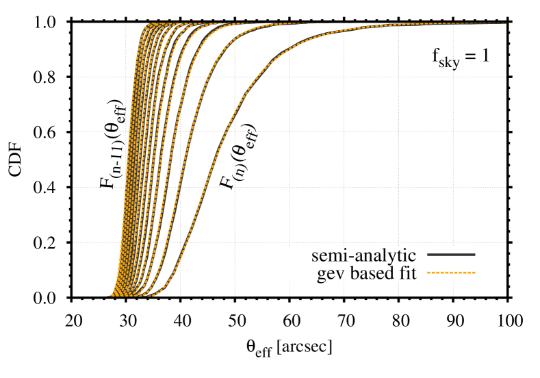
Figure 3: Cumulative distribution functions of the first twelve order statistics of the effective Einstein radius. The black solid lines depict the distributions based on the semi-analytic MC sampling of $2\,000$ Einstein radii in the redshift range of $0.5\leq z\leq 1.0$ on the full sky. The orange dashed lines denote fits of the distributions of the maxima $F_{(n)}(\theta_{\rm eff})$ with a GEV distribution.

5 Comparison with observations

5.1 The distributions of the order statistics of the effective Einstein radius

With a comparison to observed Einstein radii in mind, it is desirable to derive probability distributions of the order statistics of the effective Einstein radius. With the MC simulated data of the first twelve orders, presented in Fig. 1, we can now calculate the cdf of each order assuming full sky coverage, $f_{\rm sky}=1$. The result of this exercise is presented in Fig. 3, where the cdfs based on the MC data are presented. It can be seen nicely that the MC simulated data exhibits the steepening of the cdf with the increasing order that has also been found for the order statistics of the most massive and most distant galaxy clusters in Waizmann et al. (2012). As a result, while the first order $F_{(n)}$ is broad and allows the largest Einstein radius to be realised in a wide range, the higher orders are confined to an increasingly narrow range of radii. Therefore, the higher order cdfs can, in principle, be used to put tighter exclusion constraints based on the $n$-largest observed Einstein radii.

Because the distribution of the maxima, $F_{(n)}$, can be described by the GEV distribution from Eq. 5, we fit this functional form to the semi-analytic cdf (best-fit parameters: $\alpha_{\rm eff}=43.52\pm 0.017$, $\beta_{\rm eff}=6.14\pm 0.026$ and $\gamma_{\rm eff}=0.13\pm 0.005$). Then, using the relation from Eq. 4, we can infer the underlying distribution, $F(\theta_{\rm eff})$, which can in turn be used to derive all order statistics. The result of this operation is shown in Fig. 3. It can be seen that the fitted order statistics match the semi-analytic distributions very well, confirming the consistency of the higher order cdfs.

The twelfth largest order statistic, $F_{(n-11)}(\theta_{\rm eff})$, (leftmost cdf in Fig. 3) indicates that one expects a dozen of Einstein radii with roughly $\theta_{\rm eff}\gtrsim 30\arcsec$ on the full sky and assuming a source redshift of $z_{s}=2$. Applying order statistics to Einstein radii allows exclusion criteria to be formulated as a function of order, as presented in Fig. 4. Here, we show the dependence of different percentiles ($Q2$,$Q25$,$Q50$, $Q75$, and $Q98$) on the order. Choosing the 98-percentile as $\Lambda$CDM exclusion criterion, one would need to find approximately twenty Einstein radii with $\theta_{\rm eff}\gtrsim 30\arcsec$, ten with $\theta_{\rm eff}\gtrsim 35\arcsec$, five with $\theta_{\rm eff}\gtrsim 42\arcsec$, or one with $\theta_{\rm eff}\gtrsim 74\arcsec$ on the full sky, in order to claim tension with respect to the $\Lambda$CDM expectations. The presented exclusion criteria can be considered conservative because we modelled the distribution of Einstein radii using the simple semi-analytic method that does not incorporate cluster mergers. This choice was mainly motivated by the following reasons. Firstly and most importantly, in Paper II, we demonstrated that the precise choice of the mass function has a significant impact on the statistics of the largest Einstein radii. The Tinker et al. (2008) mass function is broadly considered to be more accurate than the original Press & Schechter (1974) mass function. However, it is a non-trivial task to self-consistently adapt merger tree algorithms to a given (empirical) mass function like the Tinker et al. (2008) mass function, among others. Secondly, we aimed to derive constraints that do not depend on the uncertainties (e.g. the simplified merger kinematics) of our semi-analytic method for modelling cluster mergers. Thirdly, the required computing time drops significantly when cluster mergers are ignored. In particular, the first two points were important for our intention to minimise model uncertainties, thereby arriving at solid and rather conservative exclusion criteria. As discussed in Paper I, cluster mergers will certainly shift the cdfs to even higher values of $\theta_{\rm eff}$. We discuss the use of the order statistical distribution for falsification experiments in more detail in the following section.

For convenience, we use the fitted distributions for the rest of this work. Any small error introduced by this choice will be negligible in comparison to the unavoidable, still present model uncertainties such as the precise shape of the mass function and the uncertainty in $\sigma_{8}$ (see Paper II, for a more detailed discussion).

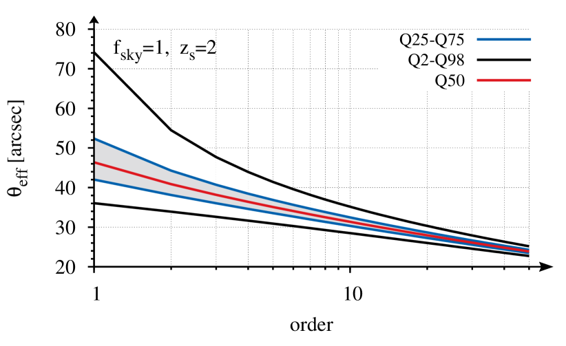
Figure 4: Dependence of different percentiles of the effective Einstein radius on the order assuming full sky coverage and a source redshift of $z_{\rm s}=2$. The red line depicts the median (Q50), the blue lines the inner quartile range (Q25-Q75), and the black lines the 2-percentile (Q2,lower curve) and the 98-percentile (Q98, upper curve). The latter can be used as $\Lambda$CDM exclusion criterion given the assumptions.

5.2 Comparison with the MACS sample

We now intend to compare the theoretical order statistics with the effective Einstein radii that are based on the strong lensing analysis of a complete sample of twelve MACS clusters by Zitrin et al. (2011) with $z>0.5$. Their parametric strong-lensing analysis (see e.g. Broadhurst et al. 2005; Zitrin & Broadhurst 2009; Zitrin et al. 2009b, for more details on the method) of HST/ACS images of all twelve objects assumes a constant source redshift of $z_{\rm s}=2$, identical to the one used for deriving the order statistics. To compare the observed sample to the order statistical distributions, we sort all Einstein radii by size and list them in Table 1.

The results of the comparison are presented in Fig. 5 in the form of a box-and-whisker diagram. Defining outliers with respect to the $\Lambda$CDM expectations as observations that exceed the $98-$percentile, none of the twelve observed Einstein radii falls outside the expectations for the full sky. That all observed Einstein radii with order larger than five fall below the $2-$percentile, with a much steeper slope, is a clear indication that the MACS sample is incomplete in terms of the largest Einstein radii that are expected to be found in the redshift range of $0.5\leq z\leq 1.0$. This is not surprising because we showed in the first part of this work that the sample of the largest Einstein radii stems from a wide range in mass and so a much larger observed sample is required to achieve completeness for the largest Einstein radii. In this sense, our conclusion is that the sample of effective Einstein radii of the studied MACS sample is consistent with the $\Lambda$CDM expectations. Furthermore, PLANCK results (Planck Collaboration et al. 2013) indicate higher values of $\Omega_{{\rm m}0}$ and $\sigma_{8}$ in comparison to the WMAP7 ones that shift the probability distributions of the different orders to higher masses, hence rendering the MACS sample even more likely to be found.

It would be interesting, though beyond the scope of this work, to extend this type of analysis to include the conditional order statistics of cluster samples that are selected given other observables.

We should note that the nominal survey area of the MACS survey comprises only a fraction of the full sky $(A_{\rm s}=22735\,{\rm deg}^{2})$, which will shift the theoretical distributions to slightly lower values of $\theta_{\rm eff}$. The conclusion from above, however, should still hold, considering that we neglected the impact of cluster mergers in our modelling (not all MACS clusters can considered to be relaxed) and, as discussed before, these events will substantially shift the expectations to higher values of $\theta_{\rm eff}$. Furthermore, a plethora of uncertainties that enter the modelling of Einstein ring distributions will, from a statistical point of view, widen the range of the theoretical distributions. Those uncertainties comprise, for example, the uncertainty of the mass function at very high masses and the uncertainty in distribution of extreme halo axis ratios, which both strongly affect the distribution of the largest Einstein radii.

Table 1: Summary of the results of the strong lensing analysis of all 12 MACS clusters by Zitrin et al. (2011) relevant for this work. The clusters are ordered by effective Einstein radius.

MACS	$z$	$\theta_{\rm eff}$	$\simeq r_{\rm eff}$	Mass
		(arcsec)	(kpc)	($10^{14}M_{\odot}$)
J0717.5+3745	0.546	$55\pm 3$	353	$7.40^{+0.50}_{-0.50}$
J0257.1-2325	0.505	$39\pm 2$	241	$3.35^{+0.58}_{-0.10}$
J2129.4-0741	0.589	$37\pm 2$	246	$3.40^{+0.60}_{-0.30}$
J0744.8+3927	0.698	$31\pm 2$	222	$3.10^{+0.10}_{-0.10}$
J0025.4-1222	0.584	$30\pm 2$	199	$2.42^{+0.10}_{-0.13}$
J0647.7+7015	0.591	$28\pm 2$	187	$2.07^{+0.10}_{-0.10}$
J1149.5+2223	0.544	$27\pm 3$	173	$1.71^{+0.10}_{-0.20}$
J0018.5+1626	0.545	$24\pm 2$	154	$1.46^{+0.10}_{-0.10}$
J2214.9-1359	0.503	$23\pm 2$	142	$1.25^{+0.10}_{-0.10}$
J1423.8+2404	0.543	$20\pm 2$	128	$1.30^{+0.40}_{-0.40}$
J0454.1-0300	0.538	$13^{+3}_{-2}$	83	$0.41^{+0.03}_{-0.01}$
J0911.2+1746	0.505	$11^{+3}_{-1}$	68	$0.28^{+0.02}_{-0.01}$

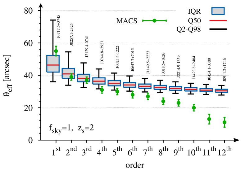
Figure 5: Box-and-whisker diagram for the comparison of the order statistics with the twelve observed effective Einstein radii of the MACS cluster sample Zitrin et al. (2011) as listed in Table 1. For each order, the red lines denote the median ($Q$50), the blue bordered grey boxes give the inner-quartile-range (IQR), and the black whiskers mark the range between the $2$ and $98-$percentile ($Q$2, $Q$98) of the theoretical distribution. The green error bars represent the observed effective Einstein radius.

5.3 Joint distributions

Apart from the study of the individual order statistics, it is also possible to derive joint distributions for different orders by means of Eq. 6 and Eq. 7. We exemplarily present the joint pdfs for combinations of the first with the ninth largest orders in Fig. 6. The pdfs are limited to a triangular domain due to the ordering constraint. It can be seen that, while for the combination with the second largest Einstein radius (upper left panel) we are more likely to find the values close to each other, for combinations with higher orders it is more likely that we find them to be realised with a larger gap. Furthermore, the peak of the joint pdf narrows for the smaller Einstein radius (y-axis) with increasing order. This is a direct result of the steepening of the cdf as shown in Fig. 3. In addition, we indicate the observed Einstein radii as the red error bars. That the red crosses fall with increasing order below the peak is a manifestation of the incompleteness of the sample as could also be seen for the individual order distributions in Fig. 5. In principle, the joint pdfs can also be extended to higher dimensions as outlined in Waizmann et al. (2013) for the order statistics in mass and redshift.

The joint pdfs shown in Fig. 6 also imply that the ratio of Einstein radii of different orders could itself be an important diagnostic. It may even be more robust than the Einstein radii themselves because perhaps the absolute calibration may drop out.

6 Summary and conclusions

In this work, a study of the order statistics of the largest effective Einstein radii has been presented. Using the semi-analytic method that we introduced in Paper I of this series, we sampled the distributions of the twelve largest Einstein radii in the redshift range of $0.5\leq z\leq 1.0$, assuming full coverage sky, the Tinker mass function, and a source redshift of $z_{\rm s}=2$. Thus, we generalise the statistical analysis of the single largest effective Einstein ring of Paper II to the one of the $n$-largest Einstein rings. Our main results can be summarised as follows.

• The order statistics of the Einstein radii allows formulating $\Lambda$CDM exclusion criteria for the $n$-largest observed Einstein radii. We find that, in order to exhibit tension with the concordance model, one would need to observe roughly twenty Einstein radii with $\theta_{\rm eff}\gtrsim 30\arcsec$, ten with $\theta_{\rm eff}\gtrsim 35\arcsec$, five with $\theta_{\rm eff}\gtrsim 42\arcsec$, or one with $\theta_{\rm eff}\gtrsim 74\arcsec$ in the redshift range $0.5\leq z\leq 1.0$, assuming full sky coverage and a fixed source redshift of $z_{\rm s}=2$.

• In the sample of semi-analytically simulated Einstein radii, the twelve largest radii stem from a wide range in mass. The sample mean in mass only slightly decreases with increasing order, while a large relative scatter of $\sim 40$ per cent is maintained. Additionally, we find that the haloes giving rise to the largest Einstein radii are on average well aligned along the line-of-sight and, with increasing rank, less triaxial. This finding supports the notion that, for the sample of the largest Einstein radii, triaxiality and halo alignment along the line-of-sight matter more than mass.

• For the sampled cdfs of the first twelve order statistics, we find a steepening of the cdfs with increasing order. This indicates that the higher orders are, in principle, more constraining. Using a GEV-based fit to the distribution of the maxima, we could show that the semi-analytic sample is self-consistent with the statistical expectation of the order statistics.

• A comparison of the theoretically expected distributions with the MACS sample shows that the twelve reported Einstein radii of Zitrin et al. (2009a) are consistent with the expectations of the concordance model. This conclusion would be consolidated further by (a) the inclusion of mergers and (b) the recent PLANCK cosmological parameters that indicate higher values of $\Omega_{{\rm m}0}$ and $\sigma_{8}$ in comparison to the WMAP7 parameters used in this analysis. Because we expect a large number of haloes to be potentially able to produce very large Einstein rings, the consistency of the studied MACS clusters with the $\Lambda$CDM expectations does not come as a surprise in view of the incompleteness of the sample.

• The method presented in this work allows calculation of joint distributions of an arbitrary combination of orders. As an example, we study the joint pdf of the two-order statistics and show that it is most likely that the largest and second largest Einstein rings are found to be realised with values very close to each other. For larger differences in the two orders, the gap between the observed values is expected to increase.

We presented a framework that allows the individual and joint order distributions of the $n$-largest Einstein radii to be derived. The presented method of formulating $\Lambda$CDM exclusion criteria by sampling the order statistical distribution is so general that it can easily be adapted to different survey areas and redshift ranges or can be included in an improved lens modelling. Such improvements will most certainly comprise the inclusion of mergers and realistic source distributions. From a statistical point of view, we do not see any evidence of an Einstein ring problem for the studied MACS sample. This conclusion is consolidated by the large uncertainties that enter the modelling of the lens distribution, which the largest Einstein radii are particularly sensitive to.

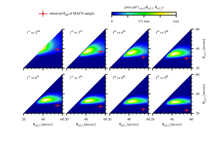
Figure 6: Pdfs of the joint two-order statistics of the effective Einstein radius for different combinations of the first with higher orders as indicated in the upper right of each panel. The distributions are calculated for the redshift range of $0.5\leq z\leq 1.0$ on the full sky. The color bar is set to range from $0$ to the maximum of the individual joint pdf in each panel. The red error bars denote the observed effective Einstein radii as listed in Table 1