A quantitative approach to evolution of music and philosophy

Abstract

The development of new statistical and computational methods is increasingly making it possible to bridge the gap between hard sciences and humanities. In this study, we propose an approach based on a quantitative evaluation of attributes of objects in fields of humanities, from which concepts such as dialectics and opposition are formally defined mathematically. As case studies, we analyzed the temporal evolution of classical music and philosophy by obtaining data for 8 features characterizing the corresponding fields for 7 well-known composers and philosophers, which were treated with multivariate statistics and pattern recognition methods. A bootstrap method was applied to avoid statistical bias caused by the small sample data set, with which hundreds of artificial composers and philosophers were generated, influenced by the 7 names originally chosen. Upon defining indices for opposition, skewness and counter-dialectics, we confirmed the intuitive analysis of historians in that classical music evolved according to a master-apprentice tradition, while in philosophy changes were driven by opposition. Though these case studies were meant only to show the possibility of treating phenomena in humanities quantitatively, including a quantitative measure of concepts such as dialectics and opposition the results are encouraging for further application of the approach presented here to many other areas, since it is entirely generic.

Keywords: Arts, music, musicology, philosophy, pattern recognition, statistics

1 Introduction

Philosophy and natural sciences were born together in the 6th century B.C. within Greek civilization [1]. Logic started with Aristotle, geometry with Thales and Euclid, arithmetic with Diophantus, while others created algebra, astronomy and politics, with all fields being part of a common knowledge space [2]. What we know today as modern philosophy and science were not originally separate, and arts were also present almost universally in this space, not only as cultural expression. The harmonic properties of music were of interest to philosophers such as Pythagoras. Aristotle with his Poetics discussed a dramatic theory for theatre. In this multidisciplinary space, music was addressed with mathematics and science with philosophy. Quantitative methods were applied to explain humanities, while the scientific method had its origin in philosophy. The segregation of this space into philosophy, science and arts was inevitable in the scientific revolution, thus leading to its division into individual, independent areas. Although specific, these areas are growing in complexity and their domains overlap. Methods from specific areas are not sufficient to deal with their complexity.

In this study, we cross the interdisciplinary borders and apply a quantitative method to philosophy and music, in an attempt to understand how humanities evolve. While philosophy and music have their history constantly analyzed and discussed by critics, the nature of their works — text documents and music scores — are difficult to analyze and interpretation is always subjective. Here we propose a generic approach to analyze features from any field in a quantitative manner. The approach, described in the next Section, was then applied to characterize composers of classical music and philosophers. The data collected from scores assigned to these composers and philosophers were treated with statistical and pattern recognition methods, with the conclusions drawn being then compared to the literature based on critics of music and philosophy.

1.1 The Approach

The approach devised to study the evolution of music and philosophy is completely generic, and can be applied to any subject. It consists of the following steps:

1. Given a subject (or area) to be studied, objects belonging to this area are identified. Here, philosophers and composers were chosen arbitrarily for the fields of philosophy and classical music, respectively. In other applications, the choice could be objective; for example, in a study of metropolitan areas the choice of the objects (cities) would obey a very precise criterion (population).

2. A set of attributes is established, which are used to characterize the objects. In our case, a few attributes were chosen arbitrarily based on well-known characteristics in the fields of philosophy and music. In order to make the analysis by humans feasible, the number of attributes had to be low. But in other types of work, the set could be chosen based on objective criteria and the number of attributes could be large.

3. For a quantitative analysis, scores are assigned for each of the attributes to each of the objects. In this study, three of the authors assigned scores based on their knowledge of the fields under study. This can be generalized, with scores assigned with objective criteria. Moreover, schemes may be applied to check the quality of the assignment, for example using the Kappa index [3] to verify agreement among the people who assigned the scores.

4. The data generated from the steps above may be sparse and in small amount, therefore unsuitable for the application of statistical methods. In order to overcome this limitation, we introduced a step to verify the robustness of the analysis, which consists in generating “artificial data” via a bootstrap method [4]. It is worth noting that in other applications, this creation of artificial data may not be needed. For instance, we could have taken data for a much larger number of philosophers and composers. However, in this paper this would hamper the task of manual score assignment, and interpretation of the final results would be much more difficult (with so many names to be analyzed).

5. Because the study is comparative, metrics must be found to identify similarities (or dissimilarities) among the objects, and projection methods are applied to visualize the data. There are several possibilities for this task, and here we used Pearson correlation and principal component analysis [5] to analyze the distances among objects. It served to establish a time line, with which the evolution of philosophy and music could be studied. Furthermore, with this time line it was possible to analyze the data in terms of concepts such as dialectics and opposition, which were obtained in a quantitative manner.

With regard to the specific methodology in the present work, we first identified prominent music composers and philosophers along history, and established a set of main musical and philosophical features. Grades were then assigned to each of the composers and philosophers for all features. The assignment of scores was not arbitrary, for they were based on research about techniques and styles used by composers and philosophers. The grades reveal a tendency index on characteristics of composers or philosophers. For example, to say that Bach is more contrapuntist than the other composers corresponds to assigning a higher grade — e.g. 8.0 or 9.0 — to the Barroque master and smaller grades to others. We chose a reduced set of philosophers and composers for the sake of simplicity and clarity. Then, to avoid statistical bias owing to the small number of samples, we developed a bootstrap method [6] with which a larger data set of 1000 new artificial composers and philosophers were generated, being directly influenced by the original sample and representing the contemporaries of the philosophers and composers chosen.

The scores assigned to the characteristics of each composer — and philosopher — define a state vector in its feature space. This quantification of composers and philosophers allowed the application of sound quantitative concepts and methods from multivariate statistics [7, 8, 9] and pattern recognition [10, 5]. Correlations between these characteristic vectors were identified and principal component analysis (PCA) [5] was applied to represent the music — and philosophy — history as a planar space where development may be followed as vectorial movements. On this planar space, concepts like dialectics, innovation and opposition, originally non-quantitative, can be modeled as mathematical relations between individual states.

It is important to note that application of statistical analysis to music is not recent. In musicology, statistical methods have been used to identify many musical characteristics. Simonton [11, 12] used time-series analysis to measure the creative productivity of composers based on their music and popularity. Kozbelt [13, 14] also analyzed productivity, but based on the measure of performance time of the compositions and investigated the relation between productivity and versatility. More recent works [15, 16] used machine-learning algorithms to recognize musical styles of selected compositions.

In contrast to the studies above, we are not interested in applying statistical analysis to music but on characterizing composers by identification of scores based on their styles. On the other hand, automatic information retrieval — that has been applied to music — is not common in philosophy. The method proposed here is a way to analyze both fields independently of the nature of their works — i.e. music pieces and textual documents — but based on a well-formed opinion of reviewers or critics on these fields and their analysis of temporal evolution.

2 Mathematical Description

Each composer or philosopher and their characteristics (i.e. opposition and skewness) are defined for each pair of subsequent composers or philosophers along time. Therefore, the choice of composers and philosophers is crucial for the time-evolution analysis. A sequence $S$ of $C$ music composers and $P$ philosophers was chosen based on their relevance in each period of classical music and western philosophy history, respectively. The set of $C$ measurements defined a $C$-dimensional space, henceforth referred to as the musical space. Likewise, we defined a $P$-dimensional philosophical space based on $P$ measurements.

The vector $\vec{v}_{i}$ for each composer or philosopher $i$ defines a corresponding composer state in the music space or philosopher state in the philosophy space. For the set of $C$ composers and $P$ philosophers, we defined the same relations summarized in Table 1. Some details about these relations are worth noting from Figure 1 for composers, and similar remarks apply to philosophers. Given a set of $C$ composers as a time-sequence $S$, the average state at time $i$ is defined as $\vec{a}_{i}$. The opposite state is defined as the “counterpoint” of a music state $\vec{v}_{i}$, considering its average state: everything running along the opposite direction of $\vec{v}_{i}$ is understood as opposition. In other words, any displacement from $\vec{v}_{i}$ along the direction $\vec{r}_{i}$ is a contrary move, and any displacement from $\vec{v}_{i}$ along the direction $-\vec{r}_{i}$ is an emphasis move. Given a composer state $\vec{v}_{i}$ and its opposite state $\vec{r}_{i}$, the opposition vector $\vec{D}_{i}$ is defined.

Table 1: Description of mathematical relations for each composer or philosopher $i$, $j$ and $k$, given a set of $C$ composers or $P$ philosophers as a time-sequence $S$. The opposition index $W_{i,j}$ quantifies how much a composer or philosopher state $i$ is opposed to $j$. The skewness index _i,j quantifies the extent to which the new composer or philosopher state $j$ departs from the corresponding opposition state. And the counter-dialectics index quantifies how much a state $k$ could be considered a synthesis between the thesis state $i$ and the antithesis state $j$.

Average state	$\vec{a}_{i}=\frac{1}{i}\sum_{k=1}^{i}\vec{v}_{k}.$
Opposite state	$\vec{r}_{i}=\vec{v}_{i}+2(\vec{a}_{i}-\vec{v}_{i})$
Opposition vector	$\vec{D}_{i}=\vec{r}_{i}-\vec{v}_{i}$
Composer or
philosopher state
move	$\vec{M}_{i,j}=\vec{v}_{j}-\vec{v}_{i}$
Opposition index	$W_{i,j}=\frac{\left<\vec{M}_{i,j},\vec{D}_{i}\right>}{||\vec{D}_{i}||^{2}}$
Skewness index	$s_{i,j}=\sqrt{\frac{|\vec{v}_{i}-\vec{v}_{j}|^{2}|\vec{a}_{i}-\vec{v}_{i}|^{2}-[(\vec{v}_{i}-\vec{v}_{j}).(\vec{a}_{i}-\vec{v}_{i})]^{2}}{|\vec{a}_{i}-\vec{v}_{i}|^{2}}}$
Counter-dialectics
index	$d_{i\rightarrow k}=\frac{|\left<\vec{v}_{j}-\vec{v}_{i},\vec{v}_{k}\right>+\frac{1}{2}\left<\vec{v}_{i}-\vec{v}_{j},\vec{v}_{i}+\vec{v}_{j}\right>|}{|\vec{v}_{j}-\vec{v}_{i}|}$

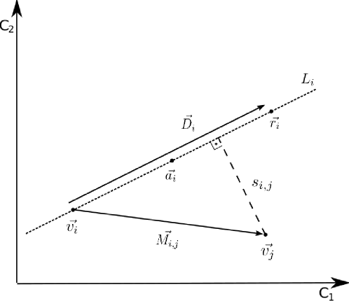
Figure 1: Graphical representation of the measures derived from a composer state move.

For the time-sequence $S$ relations between pairs of composers can be defined, as follows. The move between two successive composer states at time $i$ and $j$ corresponds to the $\vec{M}_{i,j}$ vector extending from $\vec{v}_{i}$ to $\vec{v}_{j}$. Given the composer state we can quantify the intensity of opposition by the projection of $\vec{M}_{i,j}$ along the opposition vector $\vec{D}_{i}$, normalized, yielding the opposition index $W_{i,j}$. With the same composer state, the skewness index $s_{i,j}$ is the distance between $\vec{v}_{j}$ and the line $L_{i}$ defined by the vector $\vec{D}_{i}$, thus quantifying the extent into which the new composer state departs from the corresponding opposition state. A relationship between a triple of successive composers can also be defined. Taking $i$, $j$ and $k$ as the thesis, antithesis and synthesis states, the counter-dialectics index $d_{i\rightarrow k}$ was defined by the distance between the composer state $\vec{v}_{k}$ and the middle line $ML_{i,j}$ defined by the thesis and antithesis, as shown in Figure 2. In higher dimensional musical or philosophical spaces, the middle-hyperplane defined by the points which are at equal distances to both $\vec{v}_{i}$ and $\vec{v}_{j}$ should be used instead of the middle line $ML_{i,j}$. The proposed equation for counter-dialectics scales to hyperplanes. The counter-dialectics index is used here, instead of a dialectics index, to maintain compatibility with the use of a distance from point to line as adopted for the definition of skewness.

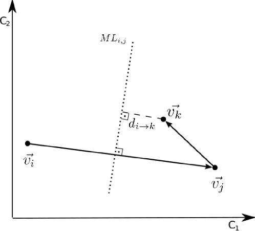
Figure 2: Graphical representation of the quantification of dialectics.

3 Characteristics

To create the music and philosophy spaces we derived eight variables corresponding to distinct characteristics commonly found in music compositions and works by philosophers. While the selected characteristics cannot be considered a summary of all the relevant features in music and philosophy history, they are initial indicators that reveal differences in style of composers and philosophers. We emphasize that the focus of this work is not on the specific characteristics used or the scores assigned, which can be disputed, but on the techniques for a quantitative analysis.

3.1 Musical Characteristics

These characteristics are related to basic elements of music — melody, harmony, rhythm, timbre, form and tessitura [17] — in addition to non-musical issues like historical events that influenced compositions, such as the importance of the Church. The eight characteristics are listed below:

Sacred - Secular ($S$-$S_{c}$): the sacred or religious music is composed through religious influence or used for its purposes. Masses, motets and hymns, dedicated to the Christian liturgy, are well-known examples [18]. Secular music has no or minimal relation with religion and includes popular songs like Italian madrigals and German lieds [17].

Short duration - Long duration ($D_{s}$-$D_{l}$): compositions quantified as short duration have a few minutes of execution. Long duration compositions have at least 20 minutes of execution. The same criterion was adopted by Kozbelt [13, 14] in his analysis of time execution.

Harmony - Counterpoint ($H$-$C$): harmony regards the vertical combination of notes, while counterpoint focuses on horizontal combinations [17].

Vocal - Instrumental ($V$-$I$): compositions using just vocals (e.g. cantata) or exclusively instruments (e.g. sonata). Note the use of vocals over instruments on Sacred compositions [18].

Non-discursive - Discursive ($D_{n}$-$D$): compositions based or not on verbal discourse, like programmatic music or Baroque rhetoric, where the composer wants to “tell a story” invoking images to the listeners mind [17]. Its contrary part is known as absolute music where music was aimed to be appreciated simply by what it is.

Motivic Stability - Motivic Variety ($M_{s}$-$M_{v}$): motivic pieces present equilibrium between repetition, reuse and variation of melodic motives. Bach is noticeable for his variation of motives, contrasting with the constantly inventive use of new materials by Mozart [19].

Rhythmic Simplicity - Rhythmic Complexity ($R_{s}$-$R_{c}$): presence or not of polyrhythms, the use of independent rhythms at the same time — also known as rhythmic counterpoint[17] — a characteristic frequently found in Romanticism and the works of 20th-century composers like Stravinsky.

Harmonic Stability - Harmonic Variety ($H_{s}$-$H_{v}$): rate of tonality change along a piece or its stability. After the highly polyphonic development in Renaissance, Webern regarded Beethoven as the composer who returned to the maximum exploration of harmonic variety [19].

3.2 Characteristics in Philosophy

We derived eight variables corresponding to some of the most recurrent philosophical issues [1, 2, 20]. Each of these variables, which defined an axis in the philosophy space, are briefly described in the following.

Rationalism - Empiricism (R-E): the rationalists claim that the human acquaintance of knowledge/concepts is significantly independent of sense experience. Empiricists understand sensory experience as the main way to gain knowledge. Empiricism is in the origin of the scientific method where knowledge must be based on sensible observation of the world instead of faith or intuition. Frequently, rationalists understand the world as affected by intrinsic properties of the human brain, in contrast to the empiricist approach where the world would imprint itself onto our minds (the principle of “tabula rasa”). For rationalists, deduction is the superior method for investigation and privileges the reason instead of experience as the source of true knowledge. Historically, Descartes, Espinoza and Leibniz introduced the rationalism in modern philosophy.

Essence - Existence (E-E): An existence-based understanding of the world has its basis on the fact that things are as an existent unit. In Existentialism, the life of an individual is determined by its self, that constitutes its essence, and not a predefined essence that defines what is to be human. Essence focuses on a substance (e.g. intellectual) that precedes existence itself. For essentialists, any specific entity has essential characteristics necessary for its function and identity. For example, to have two legs and the ability to run is not an essential characteristic defining humans, because other animals have the same characteristics. Plato was one of the first essentialists while Nietzsche and Kierkegaard were fundamental to Existentialism in the 19th century.

Monism - Dualism (M-D): Dualism requires the division of the human person into two or more domains, such as matter and soul. Monism is based on a unique “category of being”. Plato is a recognized dualist while his disciple, Aristotle, was a notable monist.

Theocentrism - Anthropocentrism (T-A): In theocentrism, God is the most important thing in the universe. The anthropocentric view has man as prevalent, with Nietzsche being its main representative. It is important to distinguish theocentrism from deism, where the figure of God is considered as an abstract entity, as for Espinoza, but does not play a central role in the universe.

Holism - Reductionism (H-R): Reductionism attempts to explain the world in terms of simple components and their emerging properties. Holists focus on the fact that the whole is more than its constitutive parts.

Deductionism - Phenomenology (D-P): Phenomenology relies on systematic reflection of consciousness and what happens in conscious acts. Deductionism is based on deriving conclusions from axiomatic systems.

Determinism - Free Will (D-F): Free will assumes that humans make choices, which are not predetermined. Determinism understands that every event is fatidic, e.g.  perfectly determined by prior states.

Naturalism - Mechanism (N-M): Methodological naturalism is the thinking basis of modern science, i.e. hypotheses must be argued and tested in terms of natural laws. Mechanism attempts to build explanation using logic-mathematical processes.

3.3 Bootstrap method for sampling

To eliminate the bias intrinsic in a small sample group, we used a bootstrap method for generating artificial composers and philosophers contemporaries of those seven chosen. The bootstrap routine generated new scores $\vec{r}$, which are not totally random because they follow a probability distribution that models the original $n=7$ scores, given by $p(\vec{r})=\sum^{n}_{i=1}e^{\frac{d_{i}}{2\sigma^{2}}}$ where $d_{i}$ is the distance between a random score $\vec{r}$ and the original score chart. For each step a value $p(\vec{r})$ is generated and compared with a random normalized value, as in the Monte Carlo [21] method to choose a set of samples. These samples simulate new randomized composers and philosophers score charts — while preserving the historical influence of the main 7 original names in each field. Higher values of $p(\vec{r})$ imply a stronger influence of the original scores over $\vec{r}$. For the analysis we used 1000 bootstrap samples obtained by the bootstrap process together with the original scores, taking $\sigma=1.1$. Other values for $\sigma$ were used yielding distributions with bootstrap samples that did not affect the music or philosophy space substantially.

4 Results and Discussion

Memorable composers were chosen as key representatives of classical music, which we believe had impact on their contemporaries, thus creating a concise parallel with music history. The chronological sequence is presented in Table 2 with each composer related to his historical period. The same was done for philosophy where a set of seven philosophers were chosen spanning the period from Classical Greece until contemporary times, and ordered chronologically as: Plato, Aristotle, Descartes, Espinoza, Kant, Nietzsche and Deleuze, as shown in Table 3.

Table 2: Sequence of music composers ordered chronologically with the period each represents.

Composer	Movement
Monteverdi	Renaissance
Bach	Baroque
Mozart	Classical
Beethoven	Classical $\to$ Romantic
Brahms	Romantic
Stravinsky	20th-century
Stockhausen	Contemporary

Table 3: Sequence of philosophers ordered chronologically with the period each represents.

Philosopher	Era
Plato	Ancient
Aristotle	Ancient
Descartes	17th-century
Espinoza	17th-century
Kant	18th-century
Nietzsche	19th century
Deleuze	20th-century

The quantification of the eight characteristics for music and philosophy was performed jointly by three of the authors of this article, based on research of history of music and western philosophy. The scores shown in Tables 4 and 5 for philosophers and composers, respectively, were numerical values between 1 and 9. Values closer to 1 reveal the composer or philosopher tended to the first element of each characteristic pair, and vice-versa.

Table 4: Quantification of eight music characteristics for each of the seven composers.

Composers	$S$-$S_{c}$	$D_{s}$-$D_{l}$	$H$-$C$	$V$-$I$	$D_{n}$-$D$	$M_{s}$-$M_{v}$	$R_{s}$-$R_{c}$	$H_{s}$-$H_{v}$
Monteverdi	3.0	8.0	5.0	3.0	7.0	5.0	3.0	7.0
Bach	2.0	6.0	9.0	2.0	8.0	2.0	1.0	5.0
Mozart	6.0	4.0	1.0	6.0	6.0	7.0	2.0	2.0
Beethoven	7.0	8.0	2.5	8.0	5.0	4.0	4.0	7.0
Brahms	6.0	6.0	4.0	7.0	4.5	6.5	5.0	7.0
Stravinsky	8.0	7.0	6.0	7.0	8.0	5.0	8.0	5.0
Stockhausen	7.0	4.0	8.0	7.0	5.0	8.0	9.0	6.0

Table 5: Quantification of eight philosophy characteristics for each of the seven philosophers.

Philosophers	R-E	E-E	M-D	T-A	H-R	D-P	D-F	N-M
Plato	3.0	3.5	9.0	5.0	4.5	3.5	5.0	4.5
Aristotle	8.0	7.5	7.0	5.5	7.5	8.0	2.5	2.5
Descartes	1.5	2.5	9.0	6.5	7.0	2.5	7.5	7.5
Espinoza	8.0	2.0	1.0	5.0	2.0	3.0	1.0	1.0
Kant	7.0	2.5	8.5	6.5	4.5	3.5	7.5	5.0
Nietzsche	7.5	9.0	1.0	9.0	5.0	8.0	1.0	1.5
Deleuze	5.5	7.5	1.0	8.0	2.5	5.5	5.0	6.0

This data set defines an 8-dimensional space for music or philosophy where each dimension corresponds to a characteristic that applies to all 7 composers or philosophers. Such small data sets are not adequate for statistical analysis, which could be biased. This is the reason why we used the bootstrap method for sampling described in section 3.3.

For the extended data set after applying the bootstrap method, Pearson correlation coefficients between the eight characteristics chosen are given in Table 6 for composers and in Table 7 for philosophers. The coefficient was 0.69 for the pairs $S$-$S_{c}$ (Sacred or Secular) and $V$-$I$ (Vocal or Instrumental), which indicates that sacred music tends to be more vocal than instrumental. The coefficient 0.56 for the pairs $S$-$S_{c}$ and $R_{s}$-$R_{c}$ (Rhythmic Simplicity or Complexity) also shows that this genre does not commonly use polyrhythms. A negative coefficient of -0.33 for the pair $V$-$I$ and $D_{n}$-$D$ (Non-discursive or Discursive) indicated that composers who used just voices on their compositions also preferred programmatic music techniques such as baroque rhetoric. Strong correlations were also observed for philosophers. For instance, the Pearson coefficient of $-0.46$ for R-E and N-M suggests that rationalists tend to be also mechanists. An even stronger correlation of $0.74$, now positive, is observed between E-E and D-P, i.e. existentialists also tend to be phenomenologists, as could be expected. Other important correlations appeared between D-F and N-M (coefficient = $0.61$) and between M-D and D-F, which seems to be directly implied by religious background.

Table 6: Pearson correlation coefficients between the eight musical characteristics. The entries with absolute values $\geq$ 0.30 have been highlighted.

-	$S$-$S_{c}$	$D_{s}$-$D_{l}$	$H$-$C$	$V$-$I$	$D_{n}$-$D$	$M_{s}$-$M_{v}$	$R_{s}$-$R_{c}$	$H_{s}$-$H_{v}$
$S$-$S_{c}$	-	-0.2	-0.06	0.69	-0.18	0.19	0.56	-0.16
$D_{s}$-$D_{l}$	-	-	-0.14	-0.13	0.2	-0.48	-0.2	0.37
$H$-$C$	-	-	-	-0.23	0.26	0.05	0.46	0.03
$V$-$I$	-	-	-	-	-0.33	0.17	0.42	-0.06
$D_{n}$-$D$	-	-	-	-	-	-0.3	0.02	-0.22
$M_{s}$-$M_{v}$	-	-	-	-	-	-	0.26	-0.15
$R_{s}$-$R_{c}$	-	-	-	-	-	-	-	-0.02
$H_{s}$-$H_{v}$	-	-	-	-	-	-	-	-

Table 7: Pearson correlation coefficients between the eight philosophical characteristics. The entries with absolute values $\geq$ 0.35 have been highlighted.

-	R-E	E-E	M-D	T-A	H-R	D-P	D-F	N-M
R-E	-	0.37	-0.23	0.15	0.1	0.46	-0.27	-0.46
E-E	-	-	-0.53	0.19	0.15	0.74	-0.61	-0.3
M-D	-	-	-	-0.43	0.41	-0.3	0.35	0.01
T-A	-	-	-	-	-0.21	0.06	0.19	0.26
H-R	-	-	-	-	-	0.32	-0.22	-0.25
D-P	-	-	-	-	-	-	-0.63	-0.47
D-F	-	-	-	-	-	-	-	0.61
N-M	-	-	-	-	-	-	-	-

The data were analyzed with principal component analysis (PCA), from which it was found that several of the characteristics contributed to the variability of the data, as shown in Tables 12 and 13 in the Supporting Information. Figures 3 and 4 display a 2-dimensional space with the first two main axes. The arrows follow the time sequence along with the seven composers and philosophers. Each of these arrows corresponds to a vectorial move from one composer or philosopher state to another. For clarity, just the lines of the arrows are preserved. The bootstrap samples define clusters around the original composers and philosophers. In subsidiary experiments, we verified that the results from the bootstrap method were robust. This was performed by applying 1000 perturbations of the original scores by adding to each score the values -2, -1, 0, 1 or 2 with uniform probability. In other words, we tested if scoring errors could be sufficient to cause relevant effects on the PCA projections. Interestingly, the values of average and standard deviation for both original and perturbed positions listed in Tables 14 and 15 in the Supporting Information show relatively small changes. It is therefore reasonable to assume that small errors in the scores assigned had no significant effect on the overall analysis.

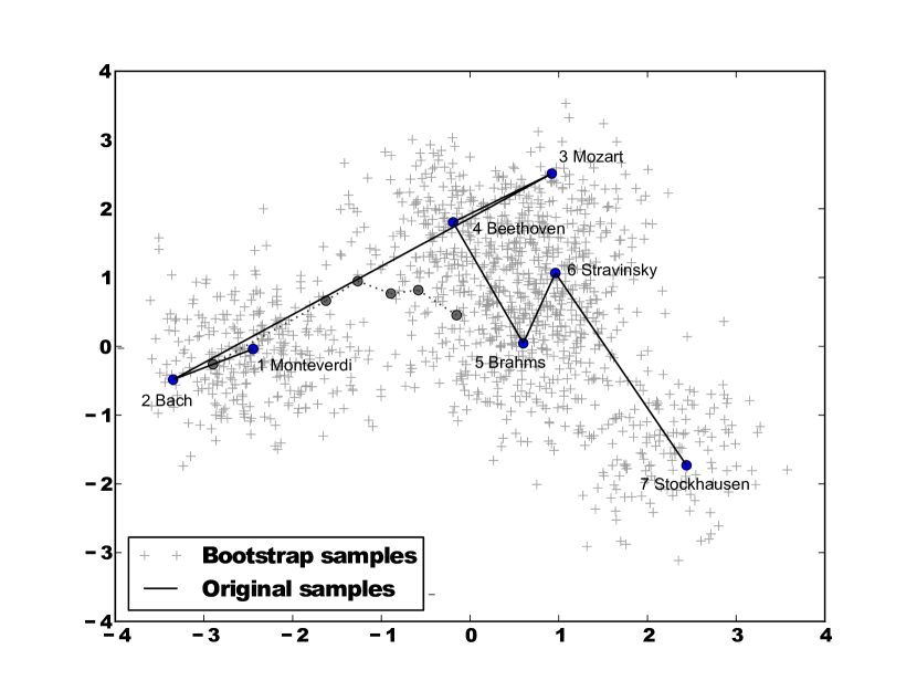
Figure 3: 2-dimensional projected music space.

Bach is found far from the rest of the composers, which suggests his key role acknowledged by other great composers like Beethoven and Webern [19]: “In fact Bach composed everything, concerned himself with everything that gives food for thought!”. The greatest subsequent change takes place from Bach to Mozart, reflecting a substantial difference in style. There is a strong relationship between Beethoven and Brahms, supporting the belief by the virtuosi Hans von Bülow [22] when he stated that the $1^{st}$ Symphony of Brahms was, in reality, the $10^{th}$ Symphony of Beethoven, appointing Brahms as the true successor of Beethoven. Stravinsky is near Beethoven and Brahms, presumably due to his heterogeneity [17, 18]. Beethoven is also near Mozart, who deeply influenced Beethoven, mainly in his early works. For Webern, Beethoven was the unique classicist who really came close to the coherence found in the pieces of the Burgundian School: “Not even in Haydn and Mozart do we see these two forms as clearly as in Beethoven. The period and the eight-bar sentence are at their purest in Beethoven; in his predecessors we find only traces of them” [19]. It could explain the move of Beethoven in direction of the Renaissance Monteverdi. Stockhausen is a deviating point when compared with the others, which could be more even so had we considered vanguard characteristics — e.g. timbre exploration by using electronic devices [18] — not shared by his precursors.

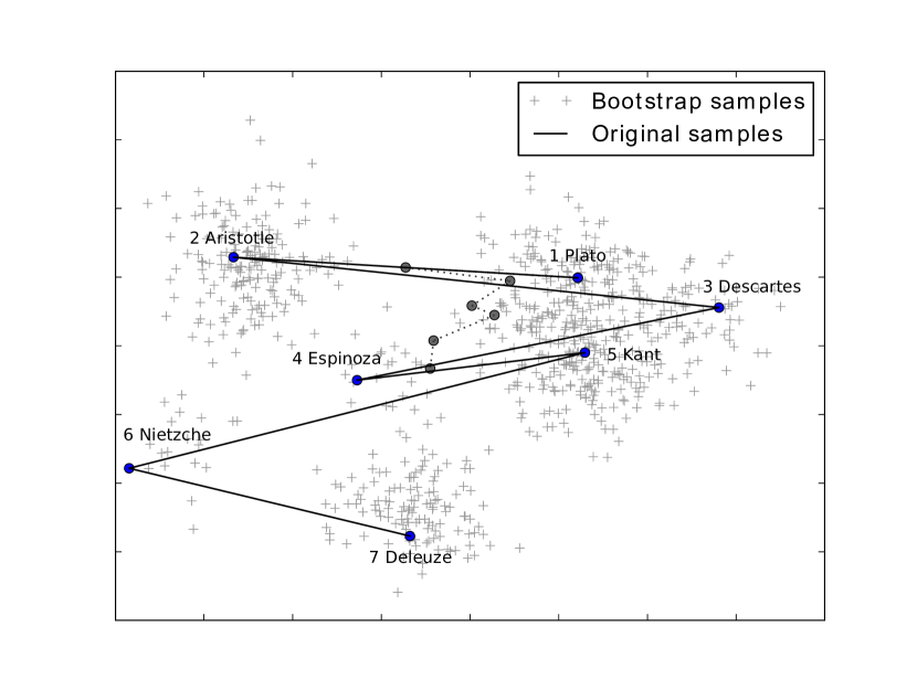
Figure 4: 2-dimensional projected philosophy space.

The opposition and skewness indices for each of the six moves among composers states in Table 8 indicate that the movements were driven by small opposition and strong skewness. In other words, most movements seem to seek innovation rather than opposition. Furthermore, the counter-dialectics indices in Table 9 are smaller than for the philosophers, as will be discussed later on.

Table 8: Opposition and skewness indices for each of the six composers states moves

Musical Move	$W_{i,j}$	$s_{i,j}$
Monteverdi $\to$ Bach	1.0	0.
Bach $\to$ Mozart	1.0196	1.9042
Mozart $\to$ Beethoven	0.4991	2.8665
Beethoven $\to$ Brahms	0.2669	1.7495
Brahms $\to$ Stravinsky	0.4582	2.6844
Stravinsky $\to$ Stockhausen	0.2516	3.1348

Table 9: Counter-dialectics index for each of the five subsequent pairs of moves among composers states for the 8 components.

Musical Triple	$d_{i\rightarrow k}$
Monteverdi $\to$ Bach $\to$ Mozart	2.0586
Bach $\to$ Mozart $\to$ Beethoven	1.2020
Mozart $\to$ Beethoven $\to$ Brahms	1.0769
Beethoven $\to$ Brahms $\to$ Stravinsky	0.2518
Brahms $\to$ Stravinsky $\to$ Stockhausen	0.2549

As for philosophy, Figure 4 shows an opposite movement from Plato to Aristotle, which confirmed the antagonistic view of Aristotle when compared with Plato, even though Aristotle was his disciple [1]. Opposition is present along all the moves among philosophers states. This oscillatory pattern makes it possible to identify two well defined groups. The first contained Aristotle, Espinoza, Nietzsche and Deleuze, in the left side of the graph. The other contained Plato, Descartes and Kant,in the right side. This division is consistent with the points of view shared by each group member. Another two groups are identified in the y-axis, separating all the philosophers from Nietzsche and Deleuze, who are represented by the most distant points.

When opposition and skewness indices in Table 10 are considered, all the moves among philosophers states tend to take place according to a well-defined, intense opposition from the average state. This was already noticeable in the PCA analysis. An interesting relationship is the minor opposition and strong skewness between Nietzsche and Deleuze, suggesting the return to Nietzsche as noted in the works of Deleuze while considering the vanguard characteristics of the 20th century philosopher [20]. Espinoza tended toward Nietzsche, and their similarity was admitted by Nietzsche, by naming Espinoza his direct precursor [1]. While similar to Espinoza, Nietzsche presented strong opposition to Kant, consistent with Nietzsche being the strongest objector to Kant ideas [1]. Also surprising was the rather small skewness among most of the moves among philosophers states, which would be driven almost exclusively by opposition to the current philosopher state. The results for dialectics in Table 11 show a progressively stronger dialectics among subsequent pairs of moves in philosophers states.

Table 10: Opposition and skewness indices for each of the six philosophers states moves.

Philosophical Move	$W_{i,j}$	$s_{i,j}$
Plato $\rightarrow$ Aristotle	1.0	0
Aristotle $\rightarrow$ Descartes	0.8740	1.1205
Descartes $\rightarrow$ Espinoza	0.9137	2.3856
Espinoza $\rightarrow$ Kant	0.6014	1.6842
Kant $\rightarrow$ Nietzsche	1.1102	2.9716
Nietzsche $\rightarrow$ Deleuze	0.3584	2.4890

Table 11: Counter-dialectics index for each of the five subsequent pairs of philosophers states moves.

Philosophical Triple	$d_{i\rightarrow k}$
Plato $\rightarrow$ Aristotle $\rightarrow$ Descartes	3.0198
Aristotle $\rightarrow$ Descartes $\rightarrow$ Espinoza	1.8916
Descartes $\rightarrow$ Espinoza $\rightarrow$ Kant	1.1536
Espinoza $\rightarrow$ Kant $\rightarrow$ Nietzsche	1.1530
Kant $\rightarrow$ Nietzsche $\rightarrow$ Deleuze	0.2705

The analysis above indicates distinct characteristics for the evolution of classical music and philosophy. Philosophers seem to have developed their ideas driven by opposition ($W_{i,j}$), as shown in Table 10, while composers tend to be more influenced by their predecessors according to the dialectics measurements ($1/d_{i\rightarrow k}$). In general, the movements among composers had minor opposition, thus reflecting the master-apprentice tradition. There is then a crucial difference in the memory treatment along the development of philosophy and music: using the same techniques, we verified that a philosopher was influenced by opposition of ideas from his direct predecessor, while composers were influenced by their two predecessors. We can argue that philosophy exhibits a memory-1 state, while music presents memory-2, with memory-N having $N$ of past generations that influenced a philosopher or composer. Furthermore, Figure 5 shows a constant decrease in the counter-dialectics index, which means a constant return to the origins for the development of music based on the search for unity. Using the words of Webern, the search for the “comprehensibility” but always influenced by their old masters.

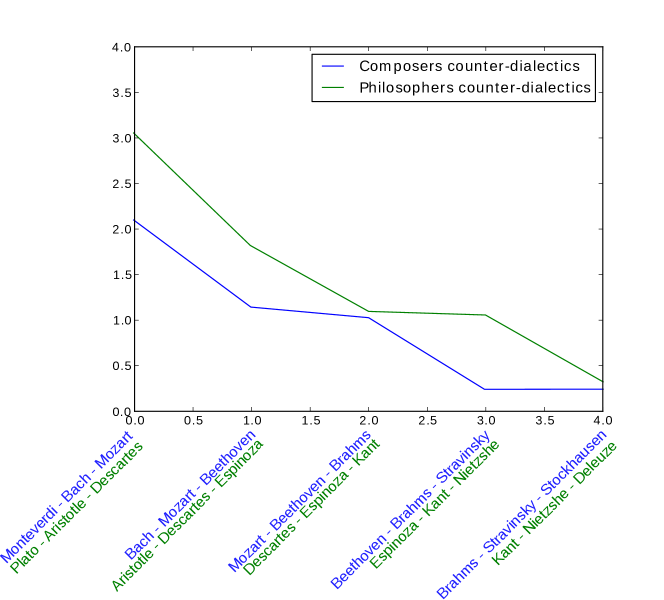
Figure 5: Comparison between composers and philosophers counter-dialectics indices

The comparison between composers and philosophers is complemented with the Wards hierarchical clustering [23], which clusters the original scores taking into account their distance. The generated dendrogram in Figure 6 shows composers according to their similarity, while the corresponding dendrogram for philosophers is shown in Figure 7. These dendrograms are consistent with the previous observations. For example, Beethoven and Brahms are close, reflecting their heritage. Stravinsky and Stockhausen form another cluster, while Mozart appears on its own, like Bach and Monteverdi. Both relations were also present in the planar space in Figure 3.

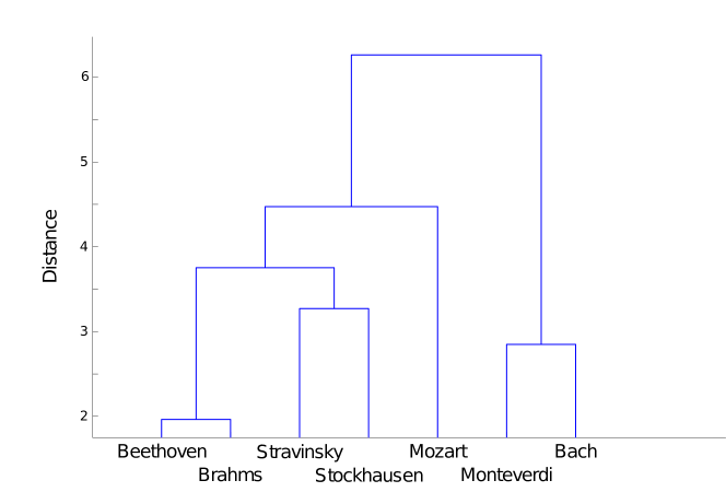
Figure 6: Wards hierarchical clustering of the seven composers.

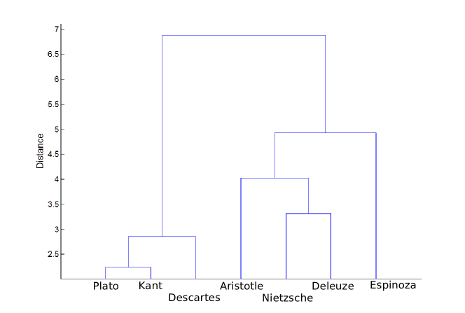
Figure 7: Wards hierarchical clustering of the seven philosophers considering all the eight features.

5 Concluding Remarks

An approach has been proposed which allows for a quantitative assessment of features from any given subject or area. For classical music and philosophy investigated here, a time line could be established based on the characteristics of composers and philosophers. The quantitative analysis involved the collection of data for these characteristics, extended with a bootstrap method to yield robustness to the statistical analysis, and the use of multivariate statistics. Also important was the establishment of indices for opposition, skewness and counter-dialectics. Though the emphasis of our work has been on the method of analysis, the interpretation of the data was already sufficient to draw conclusions that confirm intuition and subjective analyses of classical music and philosophy.

For instance, the results pointed to the development in music following a dichotomy: while composers aim at innovation, creating their own styles, their technique is based on the work of their predecessors, in a master-apprentice tradition. Indeed, in the history of music, composers developed their own styles with a continuous search for coherence or unity. In the words of Anton Webern [19], “[…] ever since music has been written most great artists have striven to make this unity ever clearer. Everything that has happened aims at this […]”. A frequent inheritance of style can be identified from one composer to another as a gradual development from its predecessor, contrasting with the necessity for innovation. Quoting Lovelock: “[…] by experiment that progress is possible; it is the man with the forward-looking type of mind […] who forces man out of the rut of ‘what was good enough for my father is good enough for me’.” [18]. In contrast, our quantitative analysis confirmed that philosophy appears to exhibit a well-defined trend in innovation: unlike music, the quest for difference seems to drive philosophical changes as expressed by Gilles Deleuze [24]. According to Ferdinand de Saussurre’s principle [25], concepts (words) tend to be different in the sense of meaning distinct things. The paradigm of difference is particularly important because it is related to the own dynamics of philosophical evolution.

Again emphasizing that our aim was to propose a generic, quantitative method, we highlight some limitations of the specific analysis made here for music and philosophy. For the scores and choice of main characteristics in music and philosophy were largely arbitrary and could be disputed. Nevertheless, the perturbation analysis performed in this work suggests that the effect of non-systematic errors in assigning the scores does not seem to be critical and has little overall impact on the conclusions drawn. Most importantly, the formal quantitative methodology described here may be combined with other methods, including information retrieval and natural language processing, to investigate other issues in humanities. For example, still connected with the present work, it can be adapted to the investigation of musical and philosophical schools, individual pieces (e.g. music suites or books), or even the contributions from the same composers or philosophers along distinct periods of time. Obviously, this methodology can also be applied to other areas such as poetry, cinema and science.

6 Acknowledgments

Luciano da F. Costa thanks CNPq (308231/03-1) and FAPESP (05/00587-5) for sponsorship. Gonzalo Travieso thanks CNPq (308118/2010-3) for sponsorship. Vilson Vieira is grateful to CAPES.

Appendix A A Brief Explanation of Principal Component Analysis (PCA)

PCA is a dimensionality reduction procedure performed through rotation of axes. It operates by concentrating dispersion/variance along the first new axes, which are referred to as the principal components. The technique consists in finding the eigenvectors and eigenvalues of the covariance matrix of the corresponding random vectors (i.e. the vectors associated with each philosophical state). The eigenvalues correspond to the variances of the new variables. When multiplied by the original feature matrix, the eigenvectors yield the new random variables which are fully uncorrelated. For a more extensive explanation of PCA, please refer to [5] and references therein.

Appendix B Supporting Information

Tables 12 and 13 show the normalized weights of the contributions of each original property on the eight axes for composers and philosophers. Most of the characteristics contribute almost equally in defining the axes.

Table 12: Percentages of the contributions from each musical characteristic on the eight new main axes.

Musical	$C_{1}$	$C_{2}$	$C_{3}$	$C_{4}$	$C_{5}$	$C_{6}$	$C_{7}$	$C_{8}$
Charac.
$S$-$S_{c}$	19.78	4.04	10.38	10.60	17.55	36.60	4.41	0.63
$D_{s}$-$D_{l}$	13.63	9.21	19.17	3.55	3.13	1.65	25.55	24.05
$H$-$C$	1.44	26.62	8.26	13.97	21.71	7.76	13.98	12.20
$V$-$I$	18.35	12.82	9.29	8.02	9.37	40.95	2.12	2.03
$D_{n}$-$D$	6.31	10.73	15.48	26.29	4.04	1.86	25.29	2.35
$M_{s}$-$M_{v}$	16.94	13.28	15.03	4.84	32.25	1.70	2.62	4.37
$R_{s}$-$R_{c}$	14.13	3.26	15.58	13.80	7.48	1.88	1.36	35.99
$H_{s}$-$H_{v}$	9.38	20.00	6.75	18.88	4.45	7.56	24.62	18.36

Table 13: Percentages of the contributions from each philosophical characteristic to the four new main axes.

Philos.	$C_{1}$	$C_{2}$	$C_{3}$	$C_{4}$	$C_{5}$	$C_{6}$	$C_{7}$	$C_{8}$
Charac.
R-E	13.35	1.81	13.11	31.12	15.06	10.99	8.20	3.56
E-E	18.13	7.88	2.10	14.68	11.41	5.31	7.98	33.50
M-D	10.07	24.59	10.71	2.91	0.69	19.39	20.95	2.91
T-A	1.08	24.18	21.51	0.68	23.72	6.31	7,27	2.06
H-R	5.90	21.49	22.29	14.90	6.35	18.81	8.69	2.05
D-P	18.99	1.29	6.85	8.41	9.67	20.50	11.47	24.93
D-F	14.57	13.67	8.37	18.93	21.12	9.06	12.77	14.98
N-M	17.86	5.06	15.03	8.33	11.96	9.59	22.62	15.97

Table 14: Averages and standard deviations for each composer and for the 8 eigenvalues.

Composers	$\mu_{\Delta}$	$\sigma_{\Delta}$
Monteverdi	3.7347	0.8503
Bach	5.3561	0.9379
Mozart	4.4319	0.8911
Beethoven	3.4987	0.7851
Brahms	3.0449	0.6996
Stravinsky	3.6339	0.7960
Stockhausen	4.2143	0.9029
Eigenvalues	$\mu_{\Delta}$	$\sigma_{\Delta}$
$\lambda_{1}$	-0.1759	0.0045
$\lambda_{2}$	-0.0638	0.0026
$\lambda_{3}$	-0.0411	0.0021
$\lambda_{4}$	-0.0144	0.0019
$\lambda_{5}$	0.0578	0.0021
$\lambda_{6}$	0.0736	0.0023
$\lambda_{7}$	0.0080	0.0027
$\lambda_{8}$	0.0835	0.0030

Table 15: Average and standard deviation for each philosopher and for the 8 eigenvalues.

Philosophers	$\mu_{\Delta}$	$\sigma_{\Delta}$
Plato	3.3263	0.7673
Aristotle	4.0896	0.8930
Descartes	4.3081	0.9225
Espinoza	4.9709	0.9131
Kant	3.2845	0.7749
Nietzsche	5.3195	0.9797
Deleuze	4.0990	0.8970
Eigenvalues	$\mu_{\Delta}$	$\sigma_{\Delta}$
$\lambda_{1}$	-0.2618	0.0068
$\lambda_{2}$	-0.0976	0.0035
$\lambda_{3}$	0.0154	0.0025
$\lambda_{4}$	0.0212	0.0024
$\lambda_{5}$	0.0697	0.0026
$\lambda_{6}$	0.0807	0.0030
$\lambda_{7}$	0.0877	0.0032
$\lambda_{8}$	0.0846	0.0036

References

References

- [1] Bertrand Russel. A History of Western Philosophy. Simon and Schuster Touchstone, 1967.
- [2] D. Papineau. Philosophy. Oxford University Press, 2009.
- [3] J. Cohen et al. A coefficient of agreement for nominal scales. Educational and psychological measurement, 20(1):37–46, 1960.
- [4] D.D. Boos. Introduction to the bootstrap world. Statistical Science, 18(2):168–174, 2003.
- [5] L. da F. Costa and R. M. C. Jr. Shape Analysis and Classification: Theory and Practice (Image Processing Series). CRC Press, 2000.
- [6] Hal Varian. Bootstrap tutorial. The Mathematica Journal, 9, 2005.
- [7] A. Papoulis and S. U. Pillai. Probability, Random Variables and Stochastic Processes. McGraw Hill Higher Education, 2002.
- [8] R. A. Johnson and D. W. Wichern. Applied Multivariate Statistical Analysis. Prentice Hall, 2007.
- [9] C. W. Therrien. Discrete Random Signals and Statistical Signal Processing. Prentice Hall, 1992.
- [10] R. O. Duda, P. E. Hart, and D. G. Stork. Pattern Classification. Wiley-Interscience, 2000.
- [11] Dean Keith Simonton. Emergence and realization of genius: The lives and works of 120 classical composers. Journal of Personality and Social Psychology, 61(5):829 – 840, 1991.
- [12] Dean K. Simonton. Creative productivity, age, and stress: A biographical time-series analysis of 10 classical composers. Journal of Personality and Social Psychology, 35(11):791 – 804, 1977.
- [13] Aaron Kozbelt. Performance time productivity and versatility estimates for 102 classical composers. Psychology of Music, 37(1):25–46, 2009.
- [14] Aaron Kozbelt. A quantitative analysis of Beethoven as self-critic: implications for psychological theories of musical creativity. Psychology of Music, 35(1):144–168, 2007.
- [15] Peter van Kranenburg. Musical style recognition – a quantitative approach. In Proceedings of the Conference on Interdisciplinary Musicology (CIM04), 2004.
- [16] Peter van Kranenburg. On measuring musical style – the case of some disputed organ fugues in the J.S. Bach (BWV) catalogue. Computing In Musicology, 15, 2007-8.
- [17] Roy Bennett. History of Music. Cambridge University Press, 1982.
- [18] William Lovelock. A Concise History of Music. Hammond Textbooks, 1962.
- [19] Anton Webern. The Path To The New Music. Theodore Presser Company, 1963.
- [20] F. G. G. Deleuze. What Is Philosophy? Simon and Schuster Touchstone, 1991.
- [21] Christian P. Robert. Simulation in statistics. In Proceedings of the 2011 Winter Simulation Conference, 2011. arXiv:1105.4823.
- [22] Alan Walker. Hans von Bülow: a life and times. Oxford University Press, 2010.
- [23] Joe H Ward Jr. Hierarchical grouping to optimize an objective function. Journal of the American Statistical Association, 58:236–244, 1963.
- [24] G. Deleuze. Difference and Repetition. Continuum, 1968.
- [25] F. de Saussure. Course in General Linguistics. Books LLC, 1916.