A Quantitative Approach to Painting Styles

Abstract

This research extends a method previously applied to music and philosophy [1], representing the evolution of art as a time-series where relations like dialectics are measured quantitatively. For that, a corpus of paintings of 12 well-known artists from baroque and modern art is analyzed. A set of 93 features is extracted and the features which most contributed to the classification of painters are selected. The projection space obtained provides the basis to the analysis of measurements. This quantitative measures underlie revealing observations about the evolution of painting styles, specially when compared with other humanity fields already analyzed: while music evolved along a master-apprentice tradition (high dialectics) and philosophy by opposition, painting presents another pattern: constant increasing skewness, low opposition between members of the same movement and opposition peaks in the transition between movements. Differences between baroque and modern movements are also observed in the projected “painting space”: while baroque paintings are presented as an overlapped cluster, the modern paintings present minor overlapping and are disposed more widely in the projection than the baroque counterparts. This finding suggests that baroque painters shared aesthetics while modern painters tend to “break rules” and develop their own style.

Keywords: Pattern recognition, arts, painting, feature extraction, creativity

1 Introduction

Painting classification is a common field of interest for applications such as painter identification — e.g. assessing the authenticity of a given art work — style classification, paintings data base search and more recently, automatic aesthetic judgment in computational creativity applications. Determining the best features for painting style characterization is a complex task on its own. Many studies [2, 3, 4, 5] applied image processing to feature extraction for painter and art movements identification. Manovich [6, 7, 8] uses features like entropy, brightness and saturation to map paintings and general images into a 2-dimensional space and, in this way, to visualize the difference between painters. There are also many related works dealing on feature selection for painting classification. Penousal et al. [9] use features based on aesthetic criteria estimated by image complexity while Zujovic et al. [10] evaluate a large set of features that most contribute to classification.

This study also analyses a set of features which most contribute to the classification of paintings. Although, in contrast with previous works, it goes forward: the historic evolution of painting styles is analyzed by means of geometric measures in the feature space. Those measures – opposition, skewness and dialectics – are central while discussing human history. However, such discussions are common only at humanities fields like Philosophy and those quantitative measures are suggested to do not surpass but contribute in this understanding of human history.

To create the feature space, a set of 93 features is extracted from 240 images of 12 well-known painters. The first six painters of this group represent the baroque movement while the remaining six represent the modern art period. A feature selection process yields the pair of features which most contributed for the classification. Similar results using LDA (Linear Discriminant Analysis) analysis are obtained, which reinforces the feature selection.

After feature selection, a centroid for each group of paintings is calculated which defines a prototype: a representative work-piece for the respective cluster. The set of all prototypes following a chronological order defines a time-series where the main purpose of this study is performed: the quantitative analysis of the historical evolution of art movements. Extending a method already applied to music and philosophy [1], opposition, skewness and dialectics measurements are taken. These concepts are central in philosophy — e.g. philosophers from antiquity like Aristotle and Plato developed their ideas using the dialectics method while it is also found in modern works like Hegelian and Marxist dialectics — and humanistic fields, however lacks studies from a quantitative perspective. [11] Represented as geometric measures, these concepts reveal interesting results and patterns. Modern paintings groups show minor superposition when compared with baroque counterparts suggesting the independence in style found historically in modernists and strong influence of shared painting techniques found in baroque painters. Dialectics and opposition values presented a peak in the transition between baroque and modern periods — as expected considering history of art — with decreasing values in the beginning of each period. Skewness index is presented with oscillating but increasing values during all the time-series, suggesting a constant innovation through art movements. These results present an interesting counterpart with previous results in philosophy — where opposition is strong in almost entire time-series — and in music — where the dialectics is remarkable [1].

The study starts describing the corpus of paintings used and a review of both aesthetic and historic facts regarding baroque and modern movements (Section 2). The image processing steps used to extract features from these paintings are presented followed by the feature selection. The results are them discussed in Section 3 with basis on geometric measurements in the projected feature space – considering the most clustered projection and LDA components.

2 Modeling painting movements

2.1 Painting corpus

A group of 12 well-known painters is selected to represent artistic styles or movements from baroque to modernism. Six painters are chosen to represent each of these movements. The group is presented in Table 1 together with their more representative style, in chronological order. It is known that painters like Picasso covered more than one style during his life. Although, only the most remarkable style is selected intending to well characterize the painter by means of this specific period or movement.

Table 1: Painters ordered chronologically with the artistic style they represents.

• artists	Remarkable Styles/Movements
  Caravaggio	Baroque, Renaissance
  Frans Hals	Baroque, Dutch Golden Age
  Nicolas Poussin	Baroque, Classicism
  Diego Velázquez	Baroque
  Rembrandt	Baroque, Dutch Golden Age, Realism
  Johannes Vermeer	Baroque, Dutch Golden Age
  Vincent van Gogh	Post-Impressionism
  Wassily Kandinsky	Expressionism, Abstract art
  Henri Matisse	Modernism, Impressionism
  Pablo Picasso	Cubism
  Joan Miró	Surrealism, Dada
  Jackson Pollock	Abstract expressionism

For each painter, 20 raw images are considered from the database of public images organized by Wikipedia. Examples of selected paintings titles and their respective creation year are listed in Table 2

Table 2: Some of the 240 selected paintings and their respective author and year of creation.

• Painter	Painting title	Year
  Caravaggio	Musicians	1595
  	Judith Beheading Holofernes	1598
  	David with the Head of Goliath	1610
  Frans Hals	Portrait of an unknown woman	1618/20
  	Portrait of Paulus van Beresteyn	1620s
  	Portrait of Stephanus Geeraerdts	1648/50
  Nicolas Poussin	Venus and Adonis	1624
  	Cephalus and Aurora	1627
  	Acis and Galatea	1629
  Diego Velázquez	Three musicians	1617/18
  	The Lunch	1618
  	La mulatto	1620
  Rembrandt	The Spectacles-pedlar (Sight)	1624/25
  	The Three Singers (Hearing)	1624/25
  	Balaam and the Ass	1626
  Johannes Vermeer	The Milkmaid	1658
  	The Astronomer	1668
  	Girl with a Pearl Earring	1665
  Vincent van Gogh	Starry Night Over the Rhone	1888
  	The Starry Night	1889
  	Self-Portrait with Straw Hat	1887/88
  Wassily Kandinsky	On White II	1923
  	Composition X	1939
  	Points	1920
  Henri Matisse	Self-Portrait in a Striped T-shirt	1906
  	Portrait of Madame Matisse	1905
  	The Dance (first version)	1909
  Pablo Picasso	Les Demoiselles d’Avignon	1907
  	Guernica	1937
  	Dora Maar au Chat	1941
  Joan Miró	The Farm	1921/22
  	The Tilled Field	1923/24
  	Bleu II	1961
  Jackson Pollock	No. 5	1948
  	Autumn Rhythm	1950
  	Blue Poles	1952

It is interesting to raise some historical and aesthetic characteristics from baroque and modern movements before entering the quantitative analysis in Section 3 where those hypothesis are further discussed. Baroque is marked by tradition, a desire to portrait the truth (found in Caravaggio, Frans Hals and Velázquez), the beauty (Poussin, Vermeer), the nature and the sacred (Caravaggio, Rembrandt). A remarkable use of light contrast (as in the “chiaroscuro” technique mastered by Caravaggio), disregarding for simple equilibrium in composition and preference for complex oppositions, both compound aesthetic characteristics which baroque artists used to represent their view of nature. The transmission of those techniques from one painter to another is common in baroque. Modernists, on the other hand, did not follow “rules”. Each modern painter employed or created new ways to represent nature. As noted by Gombrich [12]: “[they] craved for an art that does not consists of tricks that could be learn, for a style that is not a mere style, but something strong and powerful like the human passion”. Van Gogh pursued this artistic trend in his intense use of colors and the caricature aspect of his paintings. Paul Gauguin searched for “primitive” in his paintings. Others, like Seurat, applied physical properties of the chromatic vision and started painting the nature like a collection of color points, and ended creating the pointillism. Modernists created a new style for each of their experiments using their own techniques to represent a nature outside of the domains already covered by their predecessors.

2.2 Image processing

All 240 images are re-sized to 800x800 pixels and cropped to consider a region positioned in the same coordinates and with same aspect of both original paintings, and pre-processed by applying histogram equalization and median filtering with a 3-size window. Feature extraction algorithms are applied to colored, gray-scale or binary versions of images as necessary (e.g. convex-hull used a binary image, whereas Haralick texture used the gray-scale image and SLIC segmentation analysis is applied to color images). Curvature measurements are extracted from segments of paintings identified by the SLIC segmentation method [13] as presented in Figure 2. The whole process is represented schematically in Figure 1 and covers all the steps from image processing through measurements, discussed in the following sections.

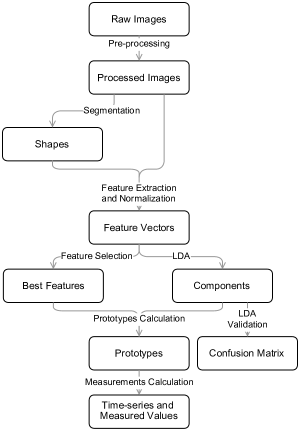
Figure 1: A summary of all steps from image processing through feature extraction through time series and measurements calculation (skewness, opposition and dialectics).

2.3 Extracted features

To create a painting space a number of distinct features extracted by computational methods from raw images of the paintings is considered. The features are related with aesthetics characteristics and aim to quantify properties well-known by art critics. All the features are summarized in Table 3 and detailed, grouped in classes, in the following list.

Table 3: Extracted features.

• Number of features	Features
  4	Energy of the whole image
  4	Energy $\mu$ of image rows
  4	Energy $\sigma$ of image rows
  4	Energy $\mu$ of image columns
  4	Energy $\sigma$ of image rows
  4	Energy centroids of image rows
  4	Energy centroids of image columns
  4	Energy $\mu$ of rows and columns
  4	Energy $\sigma$ of rows and columns
  1	$\mu$ of local entropy (5-size window)
  1	$\mu$ of local entropy (50-size window)
  4	Angular second moment
  4	Contrast
  4	Correlation
  4	Sum of squares: variance
  4	Inverse difference moment
  4	Sum average
  4	Sum variance
  4	Sum entropy
  4	Entropy
  4	Difference average
  4	Difference entropy
  2	$\mu$ of distance between curvature peaks
  2	$\sigma$ of distance between curvature peaks
  1	$\mu$ of number of curvature peaks
  1	$\mu$ of segments perimeter
  1	$\mu$ of segments area
  1	$\mu$ of circularity ($Per.^{2}/Area$)
  1	$\mu$ of number of segments
  1	$\mu$ of convex-hull area
  1	$\mu$ of convex-hull and original areas ratio
  93	Total of extracted features

General shape features: after image segmentation, a number of shape descriptors are calculated for each segment, represented as a binary matrix. Perimeter is measured as pixel-length of the segment contour. Area is estimated counting the number of pixels representing the segment. A convex-hull of the segment is used to calculate the convex area and its ratio to the original segment area. The number of constituent segments for each painting is also considered as a descriptor.

Simple complexity features: Circularity reveals how much a shape remembers a circle and is obtained by the ratio between perimeter and area of the segment. To estimate image complexity, a number of entropy measures of its energy (squared FFT coefficients) are computed — listed in the first quarter of Table 3. Together with entropy, a more specific family of measurements is considered for texture characterization: the 11 Haralick texture features [14] are calculated for this purpose.

Curvature: this descriptor has an interesting biological motivation related to the human visual system — e.g. object recognition is related to the identification of corners and high curvature points [15]. Those points have more information about object shape than straight lines or smooth curves. In this sense, curvature is well suited for the characterization of the considered paintings. Curvature $k(t)$ of a parametric curve $c(t)=(x(t),y(t))$ is defined as:

$$k(t)=\frac{\dot{x}(t)\ddot{y}(t)-\dot{y}(t)\ddot{x}(t)}{(\dot{x}(t)^{2}+\dot{y}(t)^{2})^{\frac{3}{2}}}$$ (1)

being $t$ the arc-length parameter and $\dot{x}(t)$, $\dot{y}(t)$, $\ddot{x}(t)$ and $\ddot{y}(t)$ are respectively the first and second order derivatives of $x(t)$ and $y(t)$. Those derivatives are obtained through Fourier transform and convolution theorem:

$$\dot{x}=\Im^{-1}(2\pi i\omega X(\omega))$$ (2)

$$\dot{y}=\Im^{-1}(2\pi i\omega Y(\omega))$$ (3)

$$\ddot{x}=\Im^{-1}(-(2\pi\omega)^{2}X(\omega))$$ (4)

$$\ddot{y}=\Im^{-1}(-(2\pi\omega)^{2}Y(\omega))$$ (5)

where $\Im^{-1}$ is the inverse Fourier transform, $X$ and $Y$ are the Fourier transform of $x$ and $y$ respectively, $\omega$ is the angular frequency and $i$ is the imaginary unit (see Figure 2).

The corresponding features are calculated from the curvature data: the mean and standard deviation of data, the number of peaks and the distance (geometric and in pixels) between peaks. It is important to note that a peak is defined as a high curvature point. A point $a$ is considered a peak if its curvature $k(a)$ satisfies the following criteria:

$$k(a) > k(a-1)$$ (6)

$$k(a) > k(a+1)$$ (7)

$$k(a) > \tau$$ (8)

being $\tau$ the corresponding threshold defined as

$$median\left(k\right)\gamma$$ (9)

where $\gamma$ is a factor obtained empirically as values which reveal the desired level of curvature detail.

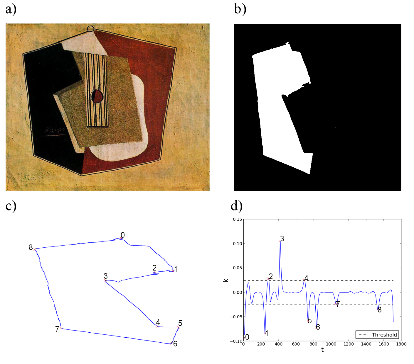
Figure 2: a) The original paintings image. b) A segmented region. c) The extracted curvature of segment. d) The parametric curve $k(t)$ with peaks given by a particular threshold.

2.4 Measurements

$N$ features define a $N$-dimensional space, also called painting space where the following measurements are calculated [1]. For simplification, a prototype $\vec{p_{i}}$ is defined for each class $C_{p}$. Each prototype summarizes a painting class, being its centroid: $\vec{p_{i}}=\frac{1}{N_{p}}\sum_{i=1}^{N_{p}}\vec{f_{i}}$ calculated in the projected space as well.

A sequence $S$ of $\vec{p_{i}}$ states defines a time series. The average state at time $i$ of states $\vec{p_{1}}$ through $\vec{p_{j}}$ is defined as:

$$\vec{a_{i}}=\frac{1}{i}\sum_{j=1}^{k}\vec{p}_{j}$$ (10)

The opposite state defines an opposition measure from $\vec{p_{i}}$ as

$$\vec{r}_{i}=\vec{p}_{i}+2(\vec{a}_{i}-\vec{p}_{i})$$ (11)

and in this way an opposition vector can be defined:

$$\vec{D}_{i}=\vec{r}_{i}-\vec{p}_{i}.$$ (12)

Knowing that any displacement from one state $\vec{p_{i}}$ to another state $\vec{p_{j}}$ is defined as

$$\vec{M}_{i,j}=\vec{p}_{j}-\vec{p}_{i}$$ (13)

it is possible to define an opposition index to quantify how much a prototype $p_{j}$ opposes $p_{i}$ (a displacement in direction of $\vec{r_{i}}$) or emphasis $p_{i}$ (a displacement in $-\vec{r_{i}}$ direction):

$$W_{i,j}=\frac{\left<\vec{M}_{i,j},\vec{D}_{i}\right>}{||\vec{D}_{i}||^{2}}$$ (14)

However, the movements in such painting space are not restricted to confirmation or refutation of “ideas”. Alternative ideas can exist out of this dualistic displacement. This is modeled as a skewness index which quantifies how much a prototype $p_{j}$ is innovative when compared with $p_{i}$:

$$s_{i,j}=\sqrt{\frac{|\vec{p}_{i}-\vec{p}_{j}|^{2}|\vec{a}_{i}-\vec{p}_{i}|^{2}-[(\vec{p}_{i}-\vec{p}_{j})(\vec{a}_{i}-\vec{p}_{i})]^{2}}{|\vec{a}_{i}-\vec{p}_{i}|^{2}}}$$ (15)

Another measure arises when considering three consecutive states at times $i,j$ and $k$. Being $p_{i}$ the thesis, $p_{j}$ the antithesis and $p_{k}$ the synthesis, a counter-dialectics index can be defined being

$$d_{i\rightarrow k}=\frac{|\left<\vec{v}_{j}-\vec{v}_{i},\vec{v}_{k}\right>+\frac{1}{2}\left<\vec{v}_{i}-\vec{v}_{j},\vec{v}_{i}+\vec{v}_{j}\right>|}{|\vec{v}_{j}-\vec{v}_{i}|}$$ (16)

or, the distance between $p_{k}$ and the middle-line (or middle-hyperplane for $N$-dimensional spaces) between $p_{i}$ and $p_{j}$. In other words, a $p_{k}$ state with higher $d_{i\rightarrow k}$ is far from the synthesis (low dialectics) and vice-versa.

2.5 Feature selection

To select the most relevant features a dispersion measure of the clusters is applied using scatter matrices [15]. For all the $N$ paintings, considering all possible combinations of feature pairs $F_{N,a}$ and $F_{N,b}$, the $S_{b}$ (between class) and $S_{w}$ (within class) scatter matrices are calculated with $K=12$ classes, one class $C_{i}$ for each painter:

$$S_{w}=\sum_{i=1}^{K}S_{i}$$ (17)

$$S_{b}=\sum_{i=1}^{K}N_{i}(\vec{\mu_{i}}-\vec{M})(\vec{\mu_{i}}-\vec{M})^{T}$$ (18)

with $N_{p}$ the number of paintings in class $C_{p}$ and the scatter matrix for class $C_{i}$ defined as

$$S_{i}=\sum_{i\in C_{i}}(\vec{f_{i}}-\vec{\mu_{i}})(\vec{f_{i}}-\vec{\mu_{i}})^{T}$$ (19)

where $\vec{f_{i}}$ is an object of the feature matrix $F$ whose rows and columns correspond to the paintings and its features $F=\left[\leftarrow f_{i}^{T}\rightarrow\right]$ and $\vec{\mu_{p}}$ and $\vec{M}$ are the mean feature vectors for objects in class $C_{p}$ and for all the paintings, respectively:

$$\vec{\mu_{p}}=\frac{1}{N_{p}}\sum_{i\in C_{p}}\vec{f_{i}}$$ (20)

$$\vec{M}=\frac{1}{N}\sum_{i=1}^{N}\vec{f_{i}}$$ (21)

The trace of within- and between-class ratio can be used to quantify dispersion:

$$\alpha=\mathrm{tr}(S_{b}S_{w}^{-1})$$ (22)

Large values of $\alpha$ reveal larger dispersion and the features which relate with large values of $\alpha$ are selected for the analysis (Section 3.1).

3 Results and discussion

3.1 Best features

By calculating $\alpha$ using Eq. 22 for all possible feature pairs $F_{N,a}$ and $F_{N,b}$ of the $N=93$ features and ordering the results by $\alpha$, it is possible to select the features which are most relevant to classification: pairs with high $\alpha$ present better dispersion and clustering than pairs with lower values. As shown in Table 4 (and Figure 3), features $\mu$ of curvature peaks and $\mu$ of number of segments have the higher $\alpha$ and are selected to opposition, skewness and dialectics analysis — both features are shown as predominant also in LDA, discussed in next section. It is interesting to note the nature of selected features: the number of segments and curvature peaks are the most prominent characteristics for the classification of paintings, even better than texture or image complexity. Other features presenting large values of $\alpha$ — like $\mu$ of convex-hull area, segments perimeter and area, and circularity — are also related with shape characteristics. Both features presented a similar projection and clustering properties of Figure 3 as showed in Figure 12.

Table 4: Feature pairs $F_{N,a}$ and $F_{N,b}$ ordered by $\alpha$. Pairs with higher $\alpha$ present better dispersion and clustering. The best feature pairs $\mu$ of curvature peaks and $\mu$ of number of segments are selected for analysis and metrics calculation.

• Pair nr.	Feature $a$	Feature $b$	$\alpha$
  1	$\mu$ of curvature peaks	$\mu$ of number of seg.	42.445
  2	$\mu$ of number of seg.	$\mu$ of convex-hull area	37.406
  3	$\mu$ of segments perimeter	$\mu$ of number of seg.	36.703
  4	$\mu$ of segments area	$\mu$ of number of seg.	36.214
  5	$\mu$ of number of segments	$\mu$ convex / original	34.885
  6	$\mu$ of circularity ($\mathrm{Per.}^{2}/\mathrm{Area}$)	$\mu$ of number of seg.	33.540
  7	Energy $\mu$ of image rows (green)	$\mu$ of number of seg.	32.954
  8	Energy $\mu$ of rows and columns (green)	$\mu$ of number of seg.	32.954
  9	Energy $\sigma$ of image rows (green)	$\mu$ of number of seg.	32.932
  10	Energy $\sigma$ of rows and columns (green)	$\mu$ of number of seg.	32.906
  11	$\mu$ of local entropy (5-size window)	$\mu$ of number of seg.	32.898
  12	Entropy (Haralick adj. 4)	$\mu$ of number of seg.	32.898
  13	Entropy (Haralick adj. 3)	$\mu$ of number of seg.	32.883
  14	Entropy (Haralick adj. 1)	$\mu$ of number of seg.	32.874
  15	Entropy (Haralick adj. 2)	$\mu$ of number of seg.	32.869
  16	Energy $\mu$ of image rows (r.)	$\mu$ of number of seg.	32.865

The projected painting space considering all the paintings that are “represented” by $\vec{p_{i}}$ is presented in Figure 3 which reveals well clustered groups with minor superposition, mainly for modern paintings. The time-series $S$ formed by prototypes $\vec{p_{i}}$ of each painter into the projected space is shown as well.

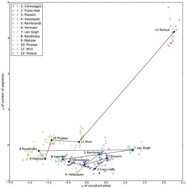
Figure 3: Projected painting space considering the best pair of features: $\mu$ of curvature peaks and $\mu$ of number of segments.

A striking result is the high distance which Pollock stays when compared with the other painters: it is a consequence of the lag number of segments present in works of Pollock (the y-axis being the projection of this feature: $\mu$ of segments number). Therefore, both the x-axis ($\mu$ of curvature peaks) and y-axis are relevant to separate the baroque and modern art movements. It is possible to note a separation between baroque and modern painters where the baroque paintings are arranged in an overlapping group while the modern painters are more clustered and separated from each other while covering a widely region of the painting space. This is confirmed by the history of art with modern painters being more individualists in their styles while baroque painters are used to share aesthetic characteristics in their paintings. The same observation arises when following the time-series, the difference between the movements is clear: while baroque artists tend to present a recurring pattern, an abrupt displacement separates Van Gogh — the first modern painter in the painting space — from the previous, and breaks the cyclic pattern. Van Gogh, although located near the baroque painters and in the opposite extreme of modern painters, represents a transition to the modern period and after him the following vector displacements will continue to evolve until reaching its apex with Pollock.

While analyzing the baroque group separately, it is possible to observe a trajectory drawn by Caravaggio and Frans Hals through Poussin which ends with the opposite (and back forth) movement of Velásquez. It can be attributed to the influence of the “chiaroscuro” master into these painters, mainly in Velásquez who is known to have studied the works of Caravaggio [12]. It arises again in the return to the Caravaggio movement by Vermeer – some critics affirm [16] that painters like Vermeer could not have even existed without Caravaggio’s influence: Vermeer and Caravaggio clusters are the most superimposed considering all the portraits in the painting space. Both facts are confirmed by the histograms of gray levels shown in Figure 4. Velazquez and Vermeer curves are more similar to Caravaggio than the remaining baroque painters.

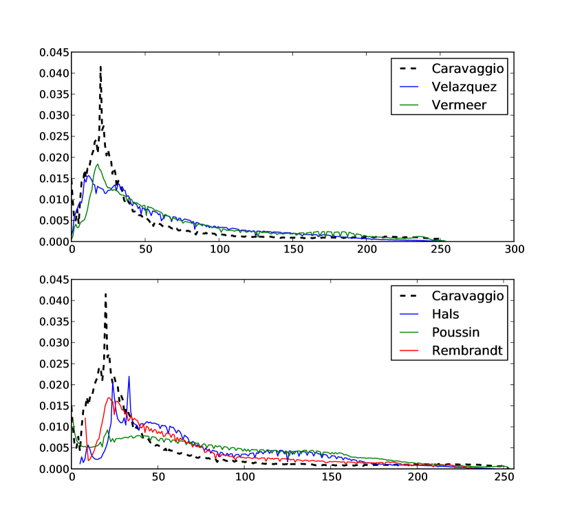
Figure 4: Mean gray levels histograms for all the baroque painters. Vermeer and Velazquez show more similarity with Caravaggio than other baroque painters.

In summary, the baroque group shows a strong inter-relationship by comparing with modern painters where the absence of super-impositions is remarkable. Again, this suggests a strong style-centric distinction among artists of the modern era while baroque artists shared techniques and aesthetic characteristics. This is also confirmed when comparing the histograms of modern paintings in Figure 5: smaller similarities are observed between the considered artists, contrasting with baroque painters shown in Figure 4.

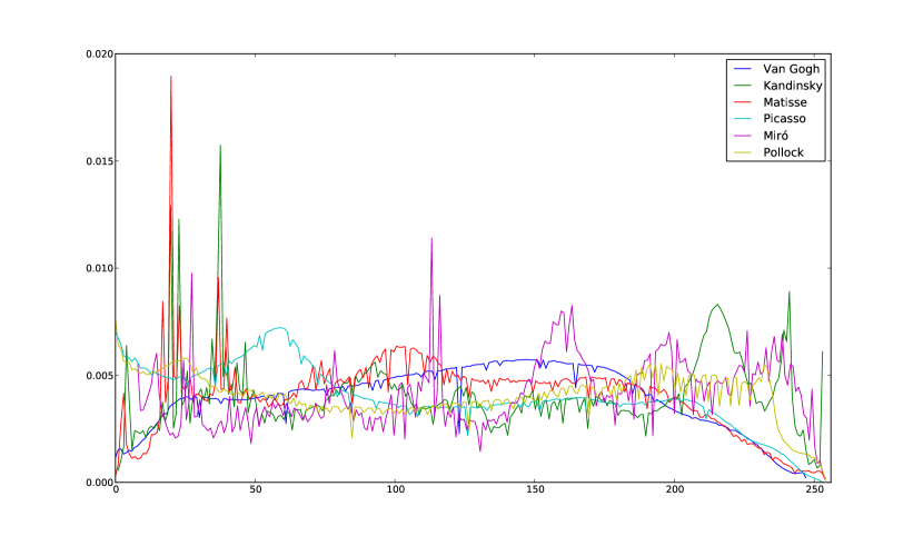
Figure 5: Mean gray levels histogram for all the modern painters. There is minor similarities between modern artists.

When considering opposition and skewness, more interesting results arise, as shown in Table 5 and Figure 6. Clearly, the larger value for opposition is attributed to Rembrandt. This is surprising given that the Dutch master figures as a “counterpoint” of baroque even being part of this art movement [12]. Vermeer also presents strong opposition and the nature of its paintings (e.g. domestic interior, use of bright colors) could explain this phenomenon. A pattern is shown in the beginning of baroque and modern art: an opposition decrease is present in both cases, which is followed by an increase in opposition. Henceforth, a following plateau of high opposition values is observed in baroque painters. This plateau happens in the transition period between baroque and modern art, gradually decreasing while the modern artists begin to take place in history. This decreasing opposition values reflects a low opposition role between first artists of baroque period and increasing opposition as long the period is moving into modernism, although skewness values remains oscillating and increasing during almost all the time-series. This characterizes again a common scene in arts, mostly in modernists, each one trying to define his own style and preparing to change into a new movement. In summary, the painting space is marked by constantly increasing skewness, strong opposition in specific moments of its evolution (the transition between baroque and modern) and minor opposition between the artists of the same movement.

Table 5: Opposition and skewness indices for each of the twelve moves for a painter to the next.

• Painting Move	$W_{i,j}$	$s_{i,j}$
  Caravaggio $\to$ Frans Hals	1.	0.
  Frans Hals $\to$ Poussin	0.111	0.425
  Poussin $\to$ Velázquez	0.621	0.004
  Velázquez $\to$ Rembrandt	1.258	0.072
  Rembrandt $\to$ Vermeer	1.152	0.341
  Vermeer $\to$ Van Gogh	1.158	0.280
  Van Gogh $\to$ Kandinsky	0.970	0.452
  Kandinsky $\to$ Matisse	0.089	0.189
  Matisse $\to$ Picasso	0.117	0.509
  Picasso $\to$ Miró	0.385	0.325
  Miró $\to$ Pollock	2.376	3.823

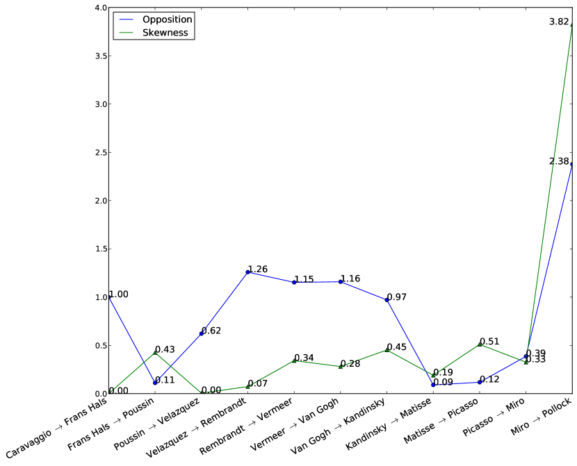
Figure 6: Opposition $W_{i,j}$ and skewness $s_{i,j}$ values for the two best features.

The counter-dialectics, shown in Table 6 and Figure 7, draws a parallel with the opposition and skewness curves. It reinforces the already observed facts: painters of the same movement show initially decreasing followed by increasing counter-dialectics reflecting the concordance of members of the same movement and their preparation to change into the next movement. The larger counter-dialectics happens in Van Gogh and Kandinsky: again, the point where baroque ends and modern art starts, regarding the painters selected for this study.

Table 6: Counter-dialectics index for each of the ten subsequent moves among painters states for the best two features.

• Painting Triple	$d_{i\rightarrow k}$
  Caravaggio $\to$ Frans Hals $\to$ Poussin	0.572
  Frans Hals $\to$ Poussin $\to$ Velázquez	0.337
  Poussin $\to$ Velázquez $\to$ Rembrandt	0.151
  Velázquez $\to$ Rembrandt $\to$ Vermeer	0.608
  Rembrandt $\to$ Vermeer $\to$ Van Gogh	1.362
  Vermeer $\to$ Van Gogh $\to$ Kandinsky	1.502
  Van Gogh $\to$ Kandinsky $\to$ Matisse	1.062
  Kandinsky $\to$ Matisse $\to$ Picasso	0.183
  Matisse $\to$ Picasso $\to$ Miró	0.447
  Picasso $\to$ Miró $\to$ Pollock	2.616

Figure 7: Counter-dialectics values considering the two best features.

3.2 All the features

Although features $F_{N,a}$ ($\mu$ of curvature peaks) and $F_{N,b}$ ($\mu$ of number of segments) showed as an interesting choice for classification, LDA is applied considering all the $N=93$ features to test the relevance of these features and the stability of the results. The LDA method [15] projected the features in a 2-dimensional space that better separates the paintings and yields a time-series as done for the two most prominent features. The first two components give the time-series shown in Figure 8. It is possible to note, as expected, a similarity with results from Subsection 3.1. The skewness indices show even more an ascending curve along the entire evolution, as presented in Table 7 and Figure 9. The opposition and dialectics (Table 8 and Figure 10) patterns remain.

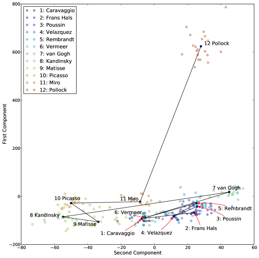
Figure 8: Time series yielded by 2-dimensional projected “painting space” considering the two first components obtained by LDA transformed into the $N=93$ feature matrix.

Table 7: Opposition and skewness indices for each of the twelve painters states moves

• Painting Move	$W_{i,j}$	$s_{i,j}$
  Caravaggio $\to$ Frans Hals	1.	0.
  Frans Hals $\to$ Poussin	-0.101	0.132
  Poussin $\to$ Velázquez	0.588	0.037
  Velázquez $\to$ Rembrandt	1.526	0.050
  Rembrandt $\to$ Vermeer	1.101	0.143
  Vermeer $\to$ Van Gogh	1.153	0.157
  Van Gogh $\to$ Kandinsky	1.279	0.512
  Kandinsky $\to$ Matisse	0.179	0.149
  Matisse $\to$ Picasso	-0.201	0.516
  Picasso $\to$ Miró	0.432	0.163
  Miró $\to$ Pollock	4.031	2.662

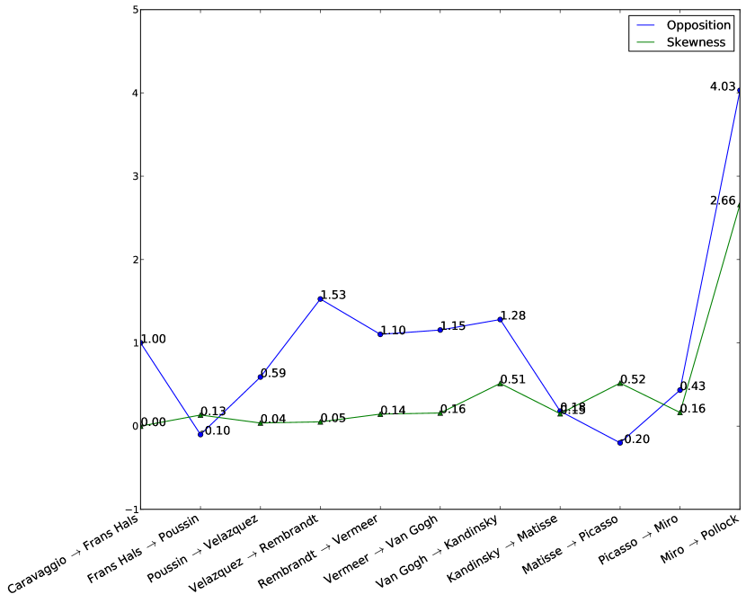
Figure 9: Opposition and Skewness values considering the time series for all the features. The same patterns observed when analyzing the best feature pair remains in this observation.

Table 8: Counter-dialectics index for each of the ten subsequent moves among painters states for the best two components of LDA projection.

• Painting Triple	$d_{i\rightarrow k}$
  Caravaggio $\to$ Frans Hals $\to$ Poussin	0.587
  Frans Hals $\to$ Poussin $\to$ Vel’azquez	0.317
  Poussin $\to$ Vel’azquez $\to$ Rembrandt	0.268
  Vel’azquez $\to$ Rembrandt $\to$ Vermeer	0.736
  Rembrandt $\to$ Vermeer $\to$ Van Gogh	1.192
  Vermeer $\to$ Van Gogh $\to$ Kandinsky	2.352
  Van Gogh $\to$ Kandinsky $\to$ Matisse	0.974
  Kandinsky $\to$ Matisse $\to$ Picasso	0.241
  Matisse $\to$ Picasso $\to$ Mir’o	0.704
  Picasso $\to$ Mir’o $\to$ Pollock	1.924

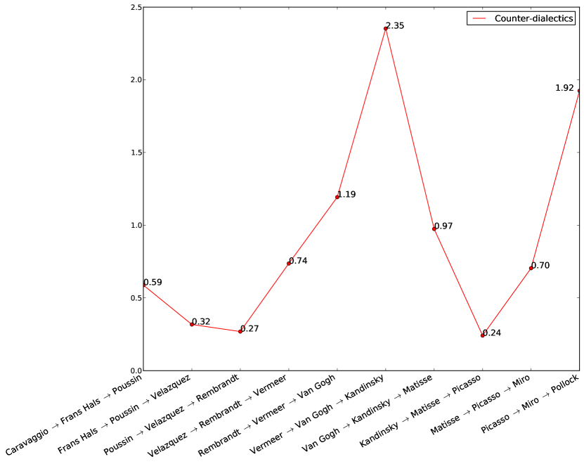
Figure 10: Counter-dialectics values (higher values reveals lower dialectics) considering all the features. The pattern observed in the best pair projection became stronger here: it is possible to observe clearly the highest value along the movement transition period (Van Gogh and Kandinsky).

For LDA validation, the total set of paintings is split in two groups: a training set with 10 random selected paintings for each artist and a test set with the remaining 10 paintings for each artist, without repetition. Such a validation is performed $100$ times. The confusion matrix (Figure 11) reveals the quality of predicted output. Diagonal elements represent the mean number of samples for which the predicted class is equal to the true class, while off-diagonal elements indicates those ones that are unclassified by LDA. Higher diagonal values indicate more correct predictions. As observed, the LDA method performed as expected for the considered set of paintings. The best classified samples are Pollock paintings which is expected given the high detachment of this cluster observed in the presented projections. In general, the confusion matrix reflects facts previously discussed: a similarity between baroque painters, mainly Velazquez, Caravaggio and Rembrandt and a separation between painters before and after Van Gogh which defines the frontier between the baroque and modern movements.

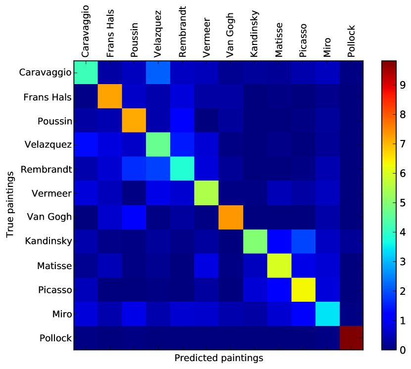
Figure 11: Confusion matrix for LDA. The half of paintings are used as a training set and the other half as test set. The validation is performed $100$ times. Diagonal elements shows the mean number of paintings in the predicted class (a painter) which equals to the true class.

4 Conclusions

It is shown that two features: a) number of curvature peaks and b) number of segments of an image — both related with shape characteristics — can be used for the classification of the selected painters with remarkable results, even when compared with canonical feature measures like Haralick or image complexity. Such relevance is supported by the analysis of a dispersion index calculated for every pair of features and reinforced by LDA analysis.

The effective characterization of selected paintings by means of these features allowed the definition of a “painting space”. While represented as states in this projected space, the baroque paintings are shown as an overlapped cluster. The modern paintings clusters, in contrast, present minor overlapping and are disposed more widely in the projection. Those observations are compatible with the history of Art: baroque painters shared aesthetics while modern painters tended to define their own styles individually [12].

A time-series — composed by prototype states representing each painter chronologically — allowed the concepts of opposition, skewness and dialectics to be approached quantitatively, as geometric measures. The painting states show a decrease in opposition and dialectics considering the first members of the same movement (baroque or modern) followed by increasing opposition and dialectics until it reaches the strong opposition momentum between the two movements. Also, the skewness curve increases during almost entire time-series. This could reflect a strong influence role of a movement in its members together with an increasing desire to innovate, present in each artist, stronger in modernists.

Both opposition, skewness and dialectics measurements can be compared with results already obtained for music and philosophy [1]. Music composers seems to be guided by strong dialectics due to the recognized master-apprentice role. Philosophers movements, otherwise, are strong in opposition. Painters, as this study reveals, show increasing skewness and strong opposition and counter-dialectics in specific moments of history.

While not sufficient to exhaust all the characteristics regarding an artist or its work, this method suggests a framework to the study of arts by means of a feature space and geometrical measures. As a future work, the number of painters could be increased and a set of painters could be specifically chosen to analyze influence (e.g. works of Frans Hals sons can be included to verify the influence of their father and master, or paintings by Rafael, Poussin and Guido Reni [12] or Carracci can be compared to confront the already known similarity of both painters). A larger number of paintings for each artist could be considered to analysis as well. The same framework can be applied to other fields of interest like Movies or Poetry. Another interesting use of this framework — being currently developed by the authors — is a component of a generative art model: geometrical measures in the painting space (like the already defined dialectics or opposition and skewness) can guide an evolutionary algorithm, assigning the value of measures as the fitness of generated material. This model complements a framework to the study of creative evolution in arts.

Appendix

Although the first features pair ($\mu$ of curvature pikes and $\mu$ of number of segments) is selected to the analysis, other features with large $\alpha$ values can be used as shown in Figure 12.

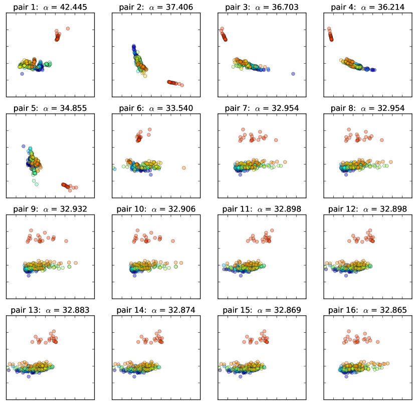
Figure 12: Scatter plots for each feature pair $i$ listed in Table 4 with large values of $\alpha$. The first projection (pair $1$) was used for the analysis, however other projections (pairs $2\ldots 16$) can be used.

References

References

- [1] Vilson Vieira, Renato Fabbri, Gonzalo Travieso, Osvaldo N Oliveira Jr, and Luciano da Fontoura Costa. A quantitative approach to evolution of music and philosophy. Journal of Statistical Mechanics: Theory and Experiment, 2012(08):P08010, 2012.
- [2] AnaIoana Deac, Jan Lubbe, and Eric Backer. Feature selection for paintings classification by optimal tree pruning. In Bilge Gunsel, AnilK. Jain, A.Murat Tekalp, and Bülent Sankur, editors, Multimedia Content Representation, Classification and Security, volume 4105 of Lecture Notes in Computer Science, pages 354–361. Springer Berlin Heidelberg, 2006.
- [3] Oguz Icoglu, Bilge Gunsel, and Sanem Sariel. Classification and indexing of paintings based on art movements. In Proc. of EUSIPCO, pages 749–752, 2004.
- [4] M. Spehr, C. Wallraven, and R. W. Fleming. Image statistics for clustering paintings according to their visual appearance. In Proceedings of the Fifth Eurographics conference on Computational Aesthetics in Graphics, Visualization and Imaging, Computational Aesthetics’09, pages 57–64, Aire-la-Ville, Switzerland, Switzerland, 2009. Eurographics Association.
- [5] C.R. Johnson, E. Hendriks, I.J. Berezhnoy, E. Brevdo, S.M. Hughes, I. Daubechies, Jia Li, E. Postma, and J.Z. Wang. Image processing for artist identification. Signal Processing Magazine, IEEE, 25(4):37–48, 2008.
- [6] Lev Manovich. Style space: How to compare image sets and follow their evolution (draft text). http://lab.softwarestudies.com/2011/08/style-space-how-to-compare-image-sets.html, August 2011.
- [7] Lev Manovich. Mondrian vs rothko: footprints and evolution in style space. http://lab.softwarestudies.com/2011/06/mondrian-vs-rothko-footprints-and.html, June 2011.
- [8] Lev Manovich. Arthistory.viz — visualizing modernism. http://lab.softwarestudies.com/2008/07/arthistoryviz-mining-200000-images-of.html, November 2008.
- [9] Juan Romero, Penousal Machado, Adrian Carballal, and Antonino Santos. Using complexity estimates in aesthetic image classification. Journal of Mathematics and the Arts, 6(2-3):125–136, 2012.
- [10] J. Zujovic, L. Gandy, S. Friedman, B. Pardo, and T.N. Pappas. Classifying paintings by artistic genre: An analysis of features and classifiers. In Multimedia Signal Processing, 2009. MMSP ’09. IEEE International Workshop on, pages 1–5, 2009.
- [11] H.L. Williams. Hegel, Heraclitus, and Marx’s Dialectic. St. Martin’s Press, 1989.
- [12] E.H. Gombrich. The story of art. STORY OF ART. Phaidon Press, Ltd., 1995.
- [13] Radhakrishna Achanta, Appu Shaji, Kevin Smith, Aurélien Lucchi, Pascal Fua, and Sabine Süsstrunk. SLIC Superpixels Compared to State-of-the-art Superpixel Methods. IEEE Transactions on Pattern Analysis and Machine Intelligence, 34(11):2274 – 2282, 2012. A previous version of this article was published as a EPFL Technical Report in 2010: http://infoscience.epfl.ch/record/149300. Supplementary material can be found at: http://ivrg.epfl.ch/research/superpixels.
- [14] Robert M Haralick, Karthikeyan Shanmugam, and Its’ Hak Dinstein. Textural features for image classification. Systems, Man and Cybernetics, IEEE Transactions on, (6):610–621, 1973.
- [15] Luciano da Fontoura Da Costa and Roberto Marcondes Cesar, Jr. Shape Analysis and Classification: Theory and Practice. CRC Press, Inc., Boca Raton, FL, USA, 1st edition, 2000.
- [16] G. Lambert and G. Néret. Caravaggio. Ediz. tedesca:. Basic Art Series. Taschen Deutschland GmbH, 2000.