Inference for feature selection using the Lasso with high-dimensional data

Abstract

Motivation: Penalized regression models such as the Lasso have proved useful for variable selection in many fields — especially for situations with high-dimensional data where the numbers of predictors far exceeds the number of observations. These methods identify and rank variables of importance but do not generally provide any inference of the selected variables. Thus, the variables selected might be the “most important” but need not be significant. We propose a significance test for the selection found by the Lasso.

Results: We introduce a procedure that computes inference and $p$-values for features chosen by the Lasso. This method rephrazes the null hypothesis and uses a randomization approach which ensures that the error rate is controlled even for small samples. We demonstrate the ability of the algorithm to compute $p$-values of the expected magnitude with simulated data using a multitude of scenarios that involve various effects strengths and correlation between predictors. The algorithm is also applied to a prostate cancer dataset that has been analyzed in recent papers on the subject. The proposed method is found to provide a powerful way to make inference for feature selection even for small samples and when the number of predictors are several orders of magnitude larger than the number of observations.

Availability: The algorithm is implemented in the MESS package in R and is freely available.

Contact: ekstrom@sund.ku.dk

1 Introduction

Molecular technologies have reached a state where it is possible to quickly and cheaply measure the status of millions of nucleotides, mRNAs, genes, proteins, or metabolites simultaneously and repeatedly over time. The availability of these massive data ideally allows for complex and detailed modeling of the underlying biological system but they also pose a serious potential multiple testing problem because the number of covariates are typically orders of magnitude larger than the number of observations. Recently, investigators are starting to combine several of these high-dimensional dataset which has increased the demand for analysis methods that accommodates these vast data (Nie et al., 2006; Brink-Jensen et al., 2013; Su et al., 2011; Kamburov et al., 2011).

As data sets increase in size, methods that promote sparse results have become more important and popular. Hastie et al. (2005) and Hesterberg et al. (2008) provide an overview of the development of these methods of which the Lasso (least absolute shrinkage and selection operator) is the most widely used (Tibshirani, 1996). While all these estimators enforce sparsity (since only a fraction of the variables are believed to be influential) and perform variable selection, they lack the inference from traditional statistics, such as $p$-values and confidence intervals. As a consequence, these models will always identify a set of the most important predictors even if none or only some of them are significant.

To address this issue several recent papers propose techniques that help asses the importance of the selected predictors. Lockhart et al. (2013) developed a method that use a covariance test statistic approach to compute $p$-values for parameters obtained from a Lasso regression. With this method $p$-values can be calculated for all predictors in a data set if there are more samples than predictors, $p<n$. In the case of $p>n$ it is not possible to use the covariance test without specifying an estimate of $\sigma^{2}$, the error standard deviation. Meinshausen et al. (2009) presents another approach where the data is split into two groups. The Lasso is applied to one group, after which the variables selected by the Lasso are used as predictors to obtain $p$-values from an ordinary least squares (OLS) regression on the other group. Wu et al. (2009) suggest to first use the Lasso to select a set of relevant variables which are then fitted to a non-penalized model where from which the $p$-values can be calculated.

In applied sciences we find often that variable selection is used for screening to determine which predictors such as genes to focus on, in further (possibly costly) analyses. A useful tool in this setting would be a model that allowed us to perform variable selection and assign a $p$-value to evaluate the evidence of the most important predictors found from the variable selection procedure. We wish to propose an approach for variable selection and inference for the Lasso that works directly when $p>n$ rather than choosing variables with Lasso and transferring these to an OLS domain for inference. Our approach uses randomization/resampling to infer the significance of the $k$th chosen predictors from a Lasso model. Thus, our focus is on using the Lasso to not only generate new (biological) hypotheses but also to evaluate the evidence for those hypotheses.

The paper is structured as follows: in the next section we present a method to both identify features and for computing $p$-values of those features obtained from a Lasso regression model. Potential problems and possible extensions are also discussed. The simulation section presents results from a series of simulation studies that show the power of the proposed method under various conditions and for situations both with and without correlated predictors. In addition we show how well the method identifies the most important of the predictors and apply the proposed method to a dataset on prostate cancer. Finally, the proposed method is discussed. Note that while we use the Lasso in the following the proposed procedure can essentially be applied in combination with any sparse feature selection approach (e.g., elastic net, ridge regression).

2 Methods

We consider the situation where we have a quantitative response vector, $\bm{y}\in\mathbb{R}^{n}$ and a set of $p$ quantitative predictors $x_{i1},\ldots,x_{ip}$ for each observation $i\in\{1,\ldots,n\}$. The number of predictors can be much larger than the number of observations, $p\gg n$ and we are interesting in identifying predictors that are associated with the response vector $\bm{y}$.

Suppose that $\bm{y}=X\bm{\beta}+\bm{\epsilon}$ where the noise is assumed to be Gaussian, $\bm{\epsilon}\sim N(0,\sigma^{2}\mathbb{I})$. The Lasso is a penalized version of the multiple regression model where sparsity of the parameter vector $\bm{\beta}\in\mathbb{R}^{p}$ is achieved by adding a penalty term to solve

$$\hat{\bm{\beta}}=\underset{\bm{\beta}\in\mathbb{R}^{p}}{\operatorname{arg\,min}}\left\{\frac{1}{2}\|\bm{y}-X\bm{\beta}\|^{2}_{2}+\lambda\|\bm{\beta}\|_{1}\right\},$$ (1)

where $\lambda\geq 0$ is the regularization parameter (Tibshirani, 1996). $\lambda$ controls the amount of shrinkage of $\hat{\beta}$ such that $\lambda=\infty$ corresponds to setting all parameters to 0, while $\lambda=0$ corresponds to an ordinary least squares multiple regression model with no restrictions on the parameter vector.

The choice of $\lambda$ will be discussed below.

The Lasso can be used for variable selection for high-dimensional data and produces a list of selected non-zero predictor variables. Meinshausen and Yu (2009) show that while the Lasso may not recover the full sparsity pattern when $p\gg n$ and when the irrepresentable condition is not fulfilled (e.g., if highly correlated predictor variables are present) it still distinguishes between important predictors (i.e., those with sufficiently large coefficients) and those which are zero with high probability under relaxed conditions.

In many high-dimensional molecular genetic datasets it is reasonable to assume that there is just a small number of genes that influence the outcome while the vast majority of genes are irrelevant for the outcome. This common setup is also relevant in other situations and it forms the basis of the following. When the relative number of truly non-zero predictors is small then the results from Meinshausen and Yu (2009) also show that the Lasso selects the non-zero parameters as well as “not too many additional zero entries of $\bm{\beta}$”. Here, we seek to identify which of the selected predictors that we believe to be non-zero. The predictors found by Lasso are generally ranked by their importance, so that a high value for $\lambda$ will include the most important predictors, decreasing $\lambda$ will include other less important predictors (Efron et al., 2004; Hastie et al., 2005; Hesterberg et al., 2008).

We wish to determine which of the features identified by the Lasso that are indeed true positives. Let $\beta_{(1)},\ldots,\beta_{(k)}$ be the ordered absolute coefficients of the $k$ non-zero predictors that are selected by the Lasso. To ensure that the effects of the predictors are comparable across variables we assume that each predictor has been standardized by dividing by their standard deviation. This is not a restriction when determining the importance of selected variables as the internal structure of the predictors (and their pairwise correlations) is preserved (Efron et al., 2004). Essentially, this approach mimics the adaptive Lasso of Zou (2006) and ensures that the coefficients are equally penalized by the $\ell_{1}$ penalty in (1). The variables can then be ordered according to their absolute size such that $|\beta_{(1)}|\geq|\beta_{(2)}|\geq\cdots\geq|\beta_{(p)}|$.

We are interested in testing hypotheses of the form

$$H_{0}:\beta_{(k)}=0,$$ (2)

where $\beta_{(k)}$ is the $k$th most important feature. Note that contrary to classical hypothesis testing we are not testing hypotheses about specific predictors but we are testing whether the $k$th identified parameter is equal to zero.

As a test statistic for the $k$th selected parameter we use the corresponding coefficient obtained from the Lasso, $|\beta_{(k)}|$. In order to derive the distribution of the $k$th identified predictor we permute response vector $\bm{y}$ to remove any associations to the set of predictors while retaining the individual structure and correlations among the set of predictors (Manly, 2006). This randomization is undertaken a large number of times and for each randomization we run the Lasso on the permuted data to obtain a distribution of coefficients for the $k$th identified predictor. Note that this approach might result in different variables being selected for each permutation and this matches the null hypothesis (2) where the focus is on finding out whether the $k$th identified predictor is significant.

The algorithm for testing the null hypothesis (2) using a randomization approach can be summarized as follows:

1. Start by scaling the predictors so their effects are comparable, i.e.,

   $$X_{j}=X_{j}/\sqrt{\mathbb{V}(X_{j})},$$

   where $X_{j}$ is the $j$th column of the design matrix $X$.

2. Fit a Lasso regression model to the original data and extract the coefficients for the selected predictors, $\hat{\beta}_{(1)},\hat{\beta}_{(2)},\ldots$.

3. Let $B$ be the (large) number of randomizations to perform to determine the distribution of the coefficients under the null hypothesis. For each $b\in B$ do the following:

   1. Permute the response vector, $\bm{y}^{b}$, and fit a new Lasso model using $\bm{y}^{b}$ as the response.

   2. Extract the coefficients for the predictors for this model, $\hat{\beta}_{(1)}^{b},\hat{\beta}_{(2)}^{b},\ldots$.

4. For each feature, $k$, we can compare the size of the coefficient identified in the original dataset, $|\hat{\beta}_{(k)}|$ to the distribution of the coefficients found for the $k$th feature for the permuted data, $|\hat{\beta}_{(k)}^{1}|,\ldots,|\hat{\beta}_{(k)}^{B}|$. The $p$-value for the $k$th feature is then the fraction of coeffients under the null that are larger than or equal to $|\hat{\beta}_{(k)}|$:

   $$p\mbox{-value}=\frac{1+\sum_{b=1}^{B}\mathbbm{1}_{|\hat{\beta}_{(k)}^{b}|\geq|\hat{\beta}_{(k)}|}}{B+1}$$ (3)

Note that by construction the $p$-value defined by (3) controls the error rate since we are simulating the distribution on the null hypothesis.

Feature selection and collinearity

In applications such as genetics, the number of predictors, $p$, is often several orders of magnitude larger than $n$ and we are typically more concerned with identifying some associations rather than finding all associations since any relationships found will often be the focus of subsequent specific experiments to verify the genetic function. Thus, our interest is on hypothesis generation rather than testing a specific hypothesis: is it possible to identity one or a few potentially interesting or relevant predictors, in a scenario with little or no knowledge of the individual predictors.

It is well-known that the Lasso has a weakness when dealing with correlated predictors: it will only select one of a group of collinear predictors to represent their effect on the response (Zou and Hastie, 2005) and the coefficient for the selected variable will have high variance (Meinshausen, 2008). Collinearity poses a problem if we are intersted in making inferences about specific predictors because the corresponding standard error becomes unstable. However, in the present setup collinearity among predictors means that while we may not be able to identify all predictors that are associated with the outcome, the size of the coefficients for the variable that are selected essentially represent the maximum effect size of the cluster of correlated predictors.

In particular, if $p\gg n$ then we may be interested in just finding one association between a predictor and the response in which case our primary focus is on the null hypothesis

$$H_{0}:\beta_{(1)}=0.$$ (4)

Choice of penalty parameter $\lambda$

The Lasso involves a penalty parameter, $\lambda$, that determines the amount of shrinkage that is applied to the parameters. In our approach, we recommend using the same procedure for estimating $\lambda$, that the reseacher would typically use together with a Lasso regularization model. Typically, $\lambda$ is determined through some form of $K$-fold cross-validation where $\lambda$ is chosen such that it minimizes the cross-validation error.

$$CV(\lambda)=\frac{1}{K}\sum_{i=1}^{N}|y_{i}-\hat{f}^{-\kappa(i)}(\bm{x}_{i},\lambda)|,$$ (5)

where $\bm{x}_{i}$ is the set of covariates for individual $i$, $\hat{f}^{-\kappa(i)}$ is the expected value from the Lasso regression based on the folds/parts of the data that does not contain observation $i$.

There are two considerations to consider here: First, we know that we are in a situation where the majority of the variables are unrelated to the outcome. Thus we want to ensure, that the majority (or possibly all) of the variables are shrunk to zero. This is particularly true under the null hypothesis where there is no association between the variables and the outcome due to randomization. Secondly, we want to ensure that when there is indeed an association between some of the variables and the outcome then we want $\lambda$ to be small enough that the effect of the associated variables are not shrunk too much.

In the following we have worked with a 10-fold cross-validation using the mean absolute error as loss function since our analyses have shown that this gives good stable results. Using the mean absolute error instead of the traditional mean squared error makes the cross-validations less sensitive to spurious extreme fits which is often the case under the null, where none of the variables are associated with the outcome. However, other approaches would be directly applicable as well at the researchers discretion.

One possible approach here, that would substantially reduce the computation time would be to use the same $\lambda$ for the randomization samples as was used in the original dataset. That ensures that we only have to do cross-validation once (for the original data) and not for each randomization. Also, the estimate of $\lambda$ under the null hypohtesis (where the randomization approach assumes that none of the predictors are associated with the outcome) can be rather unstable since there really is no obvious minimum for the cross validation procedure to reach.

Including external predictors

In some situations it is of interest to use the Lasso to select predictors from among a subset of the predictors. For example, some predictors might be related to the design of the experiment (and we wish to force them to be part of the modeling) while the remaining predictors contains the variables we wish to identify/select from because we have no prior knowledge about them.

Thus, we consider two sets of predictors, $\tilde{X}$ and $X^{\prime}$ such that $X=[\tilde{X}|X^{\prime}]$ where $\tilde{X}$ are the predictors that we wish to force into the model while $X^{\prime}$ are the predictors from which we wish to make a selection. If we apply the Lasso to $X$ we will select variables from the full set of predictors which means that some of the potential confounders that we wish to include are disregarded in the modeling.

There are two obvious alternatives to just using the classical Lasso in this situation. One is to make a two-step procedure where we first fit a model using only the predictors in $\tilde{X}$, i.e.,

$$\bm{y}=\tilde{X}\tilde{\bm{\beta}}+\bm{\epsilon}.$$ (6)

From (6) we extract the residuals, $\bm{r}=\bm{y}-\tilde{X}\hat{\tilde{\bm{\beta}}}$, and use the residuals as outcomes in combination with the procedure described above. This approach ensures that the (marginal) effects of the predictors in $\tilde{X}$ are removed and and features that are subsequently found are conditional on these marginal effects. The disadvantage is that the effects of the predictors in $\tilde{X}$ and $X^{\prime}$ are assumed to be working independently of each other, which may not be realistic.

The adaptive (or weighted) Lasso of Zou (2006) uses a weighted penalty resembling (1)

$$\hat{\bm{\beta}}=\underset{\bm{\beta}\in\mathbb{R}^{p}}{\operatorname{arg\,min}}\left\{\frac{1}{2}\|\bm{y}-X\bm{\beta}\|^{2}_{2}+\lambda\|\bm{w}\bm{\beta}\|_{1}\right\},$$ (7)

where $\bm{w}$ is a vector of non-negative weights for each predictor. Typically, the individual weights are set to $w_{j}=1/|\hat{\beta_{j}^{\prime}}|^{\nu}$, where $\hat{\beta_{j}^{\prime}}$ is the univariate regression coefficient estimate of parameter $j$ and $\nu>0$. If a weight is set to zero then the corresponding predictor will not be penalized. Thus if the weights of the parameters in $\tilde{X}$ are set to zero then the corresponding variables enter the model without being shrunk towards zero.

Family-wise error rate for multiple inference results

The $p$-value obtained from (3) controls the error rate by construction as mentioned above. However, the error rate control is on a per-hypothesis basis so if we are only aiming on making inference for the “best” selected predictor — corresponding to the hypothesis (4) — then the proposed procedure yield the correct error level.

However, in some situations it is of interest to extract inference on as many predictors as possible and simultaneously control the family-wise error rate. We can still use (3) to obtain individual $p$-values for the first feature, the second feature, etc., and Holm’s step-down procedure can control the family-wise error rate in those situations (Holm, 1979). In its original form, Holm’s procedure orders the $p$-values and makes sequential comparisons from the smallest $p$-value to the largest until the first occurrence of a null hypothesis that fails to be rejected. All other subsequent hypotheses are also not rejected.

Here we suggest a slightly different version of Holm’s procedure. The $p$-value of the $k$’th selected feature is compared against

$$\frac{\alpha}{m+1-k},$$

where $\alpha$ is the overall significance level desired and $m$ is the number of hypotheses tested. The significance level for each feature is identical to the level used by Holm’s procedure but unlike that we do not order our $p$-values according to size but test them in the order that they are selected by our procedure. This ensures that we still control the family-wise error rate (by the exact same arguments as used by Holm (1979)) since it becomes more difficult to reject hypotheses by not ordering them according to the size of the $p$-value. Also, since we keep the order of the features it prevents us from ending with a result where, say, the first and third selected features are significant but the second selected feature is not.

3 Results

Simulation studies

To examine the validity of our procedure, we performed simulation studies to assess the performance of the sensitivity and specificity. For each setting, we simulated 100 data sets with only $50$ observations generated under the linear model,

$$\bm{y}=X\bm{\beta}+\bm{\epsilon},$$

where $\bm{\epsilon}\sim N(0,\mathbb{I})$ and where $X_{ij}\sim N(0,1),\;i=1,\ldots,50,\;j=1,\ldots,p$. The unit variance is not really a restriction in this case as we start the analysis algorithm by standardizing each predictor (as outlined in the methods section above). The number of predictors were varied from 1000 to 250000 to represent various datasets.

Initially we assume that there is just a single predictor that is associated with the response and we vary the corresponding regression coefficient, $\beta$, from 0 to 1.5. This corresponds to a partial correlation coefficient between the predictor and the outcome ranging from 0 to 0.83. With these data we follow the procedure described above where each combination of predictors, $p$, and associated coefficient, $\beta$, is run 100 times and for each combination we use 100 permutations to determine the power of the feature identified as the most important corresponding to the hypothesis $\beta_{(1)}=0$. In all computations a significance level of $\alpha=0.05$ was used. In order to see how collinearity influences the power we run simulations with the same association between a single predictor and the outcome but we let that predictor be part of a cluster of ten correlated predictors such that $\mbox{cor}(X_{i},X_{i^{\prime}})=\rho$. Here, $\rho=0.5$ or $\rho=0.95$ to represent moderately and highly correlated predictors.

We first focus on two primary abilities of the model: the power to identify the first selected predictor and the impact of correlated predictors in the model. The simulation results are shown in Figure 1. The simulations show three clear results: 1) for moderate to high effect size (i.e., when $\beta$ is 1–1.5) we obtain a high power even when the number of predictors is large, 2) when the causal gene is part of a correlated cluster of predictors then the power is higher than if the gene is independent, and 3) generally there is a fall in power as the number of predictors increase although this drop appears to stabilize and level off as the set of predictors increases.

The power is 100% for an effect size of 1 or 1.5 (the lines overlay each other in Figure 1) except for the independent predictors. That means that even when there is a ratio of predictors to observations, $p/n$, of 5000 then we are still able to identify a signal in the data even with just 50 observations. An effect size of 1 corresponds to an effect of 1 standard deviation so we are even able to identify the presence of a gene with realistic biogical effects.

For correlated data we see that the power is larger than the power observed from independent predictors. This is caused by the fact that the causal predictor is part of a cluster; with correlated predictors, then each of the predictors in the cluster has a probability of showing an improved association to the outcome just by chance. Thus, we essentially improve our power to detect one of the predictors in the cluster at the cost of perhaps not detecting the true one but at least one that is highly correlated to it. If the causal predictor was a singleton and not part of a cluster of correlated predictors then the power results resemble the results from the uncorrelated data (results not shown).

Initially the power drops for all situations as the number of predictors increase (making it harder to identify that there is in fact a true association among one of the predictors and the outcome) but the overall power seems fairly constant once the number of predictors reach around 50000 (of which just one is associated with the outcome). Not surprisingly, this drop is more noticeable when the true association has a moderate effect than when the effect is smaller (where the power is consistently low) or larger (where the power is consistently high). Figure 1 also shows that we are generally able to control the family-wise error rate at the desired significance level (0.05). Perhaps most surprisingly is the consistent high power for moderate to high effect sizes ($\beta=1$ or $\beta=1.5$) considering this is based on just 50 observations.

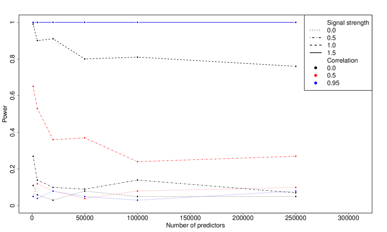
Figure 1: Power to detect the first identified predictor selected by the Lasso for varying number of predictors and varying effect size of the predictor for a dataset containing 50 observations. Each point is the average from 100 simulations, each using 100 randomizatons to compute the $p$-value. The black lines correspond to completely independent predictors, the red lines are when there is some collinearity between a group of predictors while the blue lines represent the situation with a group of highly correlated predictors.

Figure 1 focused on the evidence of the first/most important predictor. Once that has been identified we would like to determine the power to detect the second most important predictor and its power. In our simulations we assumed that there was always one causal predictor with a corresponding parameter of $\beta_{1}=1.5$ and we varied the effect of another predictor, $\beta_{2}$, with values ranging from 0 to 1.5 as previously. Following the setup above we also allow for correlations and assume that the two predictors are actually part of the same cluster.

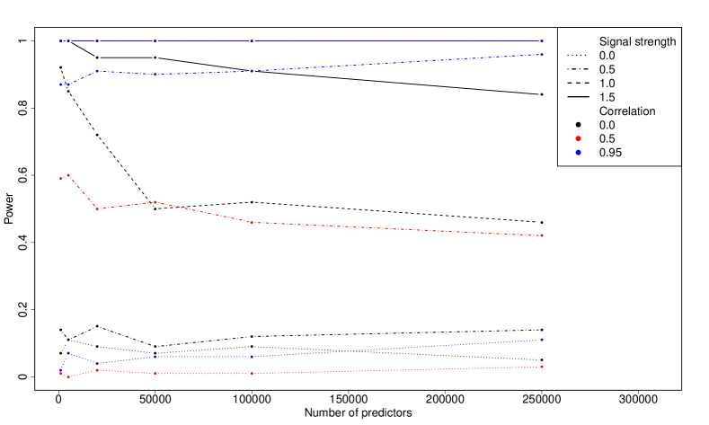
Figure 2: Power to detect the second identified predictor selected by the Lasso for varying number of predictors and varying effect size of the predictor for a dataset containing 50 observations. The dataset contains two predictors from the same group/cluster that are associated with the response, one of which is fixed with an effect size of 1.5. Each point is the average from 100 simulations, each using 100 randomizatons to compute the $p$-value. The black lines correspond to completely independent predictors, the red lines are when there is some collinearity between a group of predictors while the blue lines represent the situation with a group of highly correlated predictors.

Figure 2 shows the power to detect the second most important variable when there are two potential causal variables from the same cluster. Overall, we see the same trends as we saw for the most important variable in Figure 1 except that the power is generally lower. Looking at the solid line corresponding to the largest effect of the second most important variable we see a marked decline in power as the number of predictors increase if the predictors are all independent. The decline is not very surprising as both of the two causal predictors have the same effect size (both $1.5$) so the second most important variable will by design be the smallest of those two (after sampling error has been added). Thus, due to random variation, the estimated effect of the second is likely to be slightly smaller than the true effect (ie., biased downward) and contrary the effect of the most important variable will be slightly biased upward. However, the drop in power for the second most important variable is still substantial even for high effect sizes except when the predictors are correlated. Figure 2 also shows that the error rate is controlled around the 5% level for independent predictors when there is only one predictor that is truly associated to the response (black dotted line). As for the results from the first identified predictor, Figure 1, we get that correlated predictors increase the power to identify subsequent predictors.

As highlighted in the methods section, the proposed procedure computes the evidence for the identified features but does not directly provide significance inference for a particular predictor. In practice, however, it is also of interest how well the Lasso approach identifies the predictors, that are truly associated with the response. While this has been investigated in several papers (Efron et al., 2004; Hastie et al., 2005; Hesterberg et al., 2008; Meinshausen et al., 2009), we include results using the same simulation setup as described above for direct comparison with the simulation results shown in Figure 1. The results are shown in Figure 3 which clearly shows that the precision increases with increasing signal strength and decreases when the true predictor is part of a cluster of predictors. In the latter case, it is generally one of the the predictors from the correlated cluster that is identified, so while we may not identify the specific variable we do identify the cluster (results not shown).

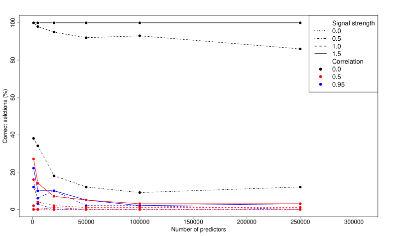
Figure 3: Feature identification precision for the Lasso to identify the single true underlying (most significant) predictor for varying number of predictors and effect sizes. Each point is the average from 100 simulations. The black lines correspond to completely independent predictors, the red lines are when there is some collinearity between a group of predictors while the blue lines represent the situation with a group of highly correlated predictors.

Application to prostate cancer data

We apply our proposed method to the prostate cancer example from Lockhart et al. (2013), a subset of 67 samples and 8 predictors from a larger dataset. The outcome is the logarithm of a prostate-specific antigen and we want to determine the association between the outcome and any predictors. Data can be found at www-stat.stanford.edu/~tibs/ElemStatLearn/. The setup for this dataset is simpler than the situation mentioned in methods section since $p<n$ so it is possible to analyze all predictors simultaneously by using, say, a classical multiple regression model. We compare the results from our proposed method with three other analyses approaches: simple multiple regression, using the Lasso in combination with the covariance test statistic of Lockhart et al. (2013) and the multi-split method of Meinshausen et al. (2009). The multi-split method essentially consists of variant of 2-fold cross-validation: First, Lasso regression is applied to a part of the dataset to select a list of predictors, and secondly an ordinary multiple regression (using the selected predictors) is applied to the remaining data to obtain $p$-values for the selected predictors.

Note that unlike our proposed approach, both the multiple regression, the Lasso-covariance test, and the multi-split method are all designed to test hypotheses about each specific predictor. However, the multi-split method is vulnerable to the selection obtained from the first split which gives rise to rather substantial variance of the $p$-values in this dataset. Splitting the sample repeatedly and getting a set of $p$-values has also been suggested by the authors, but “it is not obvious, though, how to combine and aggregate the results.” (Meinshausen et al., 2009). Here, we have just averaged the $p$-values obtained for each of the sets (with non-selected predictors getting a $p$-value of 1).

Table 1: Table of $p$-values for each predictor obtained from simple linear regression (LR), multiple regression (OLS), the multi-split method (SPLIT), the covariance test method (COV) and the proposed method (RAND). Last column shows the marginal Pearson correlation between each predictor and the outcome. Predictors are listed in order they are selected by the randomization procedure.

Predictor	LR $p$	OLS $p^{\ast}$	COV $p$	SPLIT $p$	RAND $p$	Correlation with outcome
lcavol	0.00	0.00	0.00	0.00	0.00	0.73
svi	0.00	0.05	0.17	0.29	0.34	0.56
lweight	0.00	0.00	0.05	0.06	0.14	0.49
lcp	0.00	0.09	0.05	0.89	0.07	0.49
pgg45	0.00	0.24	0.35	0.86	0.01	0.45
lbph	0.03	0.05	0.92	0.51	0.01	0.26
age	0.06	0.14	0.65	0.92	0.04	0.23
gleason	0.00	0.88	0.97	0.97	0.58	0.34
∗ $p$-values for OLS are shown after backward elimination.

Table 1 shows that the three methods that accommodate multiple predictors and test hypotheses about each specific predictor (OLS, multi-split and the covariance test) generally give the same results and all identify the same predictor, lcavol, as being the most important. The same result is obtained with our proposed method, where the first selected variable is highly significant (and turns out to be lcavol). The simple marginal regression analyses show that virtually all predictors are associated with the response, but the other approaches reduce the number of significant variables partly due to correlation among the predictors. Our proposed randomization test identifies slightly more variables than the covariance test (and a few more than the multi-split procedure) and seems to lie somewhere between the ordinary multiple regression model and the covariance test.

It is only the covariance test that places any real emphasis on the lcp predictor in part because of a high degree of collinearity to lcavol (the correlation coefficient between lcavol and lcp is $0.692$, which is the second largest among the predictors). The largest pairwise correlation is between pgg45 and gleason and is 0.757 but the association to the outcome is less for those two variables so the impact of their collinearity on the $p$-values is less noticeable.

4 Discussion

We have proposed an algorithm to aid in making inference and subsequently relevant hypotheses concerning data with (many) more predictors than samples. It greatly extends the results from shrinkage regression methods to be able to assign a $p$-value to findings from regularized regression methods that combine variable selection and estimation.

When the number of predictors $p$ is larger than then sample size $n$, regularized regression methods can be used to identify a sparse model and to provide stable parameter estimates. The standard Lasso suffers from several problems in this regard, in particular that it is not consistent in cariable selection and that the limiting distribution of the estimates are non-standard and cannot be directly derived. To overcome these shortcomings Fan and Li (2001) and Zou (2006) have presented versions of regularized regression that not only have asymptotic oracle properties but also have consistency in variable selection and asymptotic normality of the estimators. However, inference based on these improved regularization methods for finite samples generally perform poorly even when the effects are large (Minnier et al., 2011).

An obvious difference between the $p$-values obtained from ordinary least squares or from other regularized regression inference approaches is that we pursue investigating a null hypothesis that is not concerned with a specific (set of) predictor(s) but is concerned solely with evaluating the evidence that the results obtained from regularized regression are stronger than what would be expected if none of the predictors were associated with the response. Classical OLS-style $p$-values are extremely useful but it can be argued that for the majority of problems in genomics — where there is often little or no prior information about any of the possible predictors — the focus is on hypothesis generation and variable selection and not on testing specific hypotheses. Hence our focus (and the proposed procedure) is on hypothesis generation and not on inferences about specific variables.

Our simulations show that — even with just 50 observations — the proposed procedure has substantial power to identify at least one associated predictor among a set of 50–250 thousand predictors without serious performance decline (Figure 1). This suggests that not only can we can identify relevant predictors within a large set of irrelevant predictors — we can also attach a level of significance so we can evaluate whether our findings are indeed likely to be true (and relevant) predictors, that are associated to the outcome. Our results extend to the situation where there are multiple causal variables (Figure 2) although the power declines slightly more rapidly with the number of predictors when testing the importance of subsequent features. The results regarding the second most important variable shown in Figure 2 was based on two causal variables in the same cluster. If we run the same analyzes where the two causal variables are in two different clusters we get essentially the same results as shown for the uncorrelated data in Figure 2 (results not shown).

We have run the same simulations with a reduced dataset of 30 observations instead of 50 observations and while the power obviously is lower we see the same overall trends as shown above. Thus, even with fairly small datasets we have decent power to identify a variable that truly is associated to the outcome.

It can be argued that for genetic data where many genes may follow a similar pattern of expression and thus be correlated, Lasso is not an obvious choice for variable selection. If the purpose of the selection is indeed to identify a whole cluster of co-expressed genes, other shrinkage algorithms could be better suited. However if the genes selected by the Lasso are seen as the most influential representative of a cluster there are numerous ways to identify others in the same cluster. Since the whole nature of our approach is not to identify specific variables this is not a problem per se. In fact, Figures 1 and 2 show that the power to detect something from a clustered set of predictors rise dramatically so clustered predictors will just increase our power to identify at least one of the predictors from the cluster.

When comparing methods applied to the prostate dataset, it was clear that all four methods (the proposed approach, ordinary least squares, the covariance test statistic, and the split method) are able to identify the variable lcavol as among the most important and a small $p$-value is assigned to this predictor. Note that while the four methods differ somewhat in their results they also test different versions of the null hypothesis. The split method consistenly assigns a small $p$-value to the lcavol predictor but the remaining seven predictors obtain $p$-values estimated with very large uncertainties. The randomization approach generally yields lowest $p$-values which is partly due to the fact that the variables are indeed mostly correlated with the outcome, and partly due to that the null hypothesis is different (in particular it assumes that none of the predictors are associated with the outcome).

We believe the proposed method could also be applied in for instance Genome-Wide Association Studies (GWAS), where Lasso is already widely used, but significance testing typically done outside the Lasso domain, as done by Wu et al. (2009).

5 Conclusion

We have presented a method that can be used to make inference about variable selection results from regularized regression models such as the Lasso. We show that it has high power to infer evidence that the selected features are not chance findings — even when the number of predictors is several orders of magnitude larger than the number of observations, i.e., when $p>n$. The method controls the family-wise error rate and can essentially be used with any regularization method. The proposed method is relevant for situations where regularized regression methods is used as part of the statistical modeling to identify features for subsequent analyses.

References

- Brink-Jensen et al. (2013) Brink-Jensen, K., Bak, S., Jørgensen, K., and Ekstrøm, C. T. (2013). Integrative analysis of metabolomics and transcriptomics data: A unified model framework to identify underlying system pathways. PLoS ONE, 8(9), e72116.
- Efron et al. (2004) Efron, B., Hastie, T., Johnstone, I., and Tibshirani, R. (2004). Least angle regression. The Annals of statistics, 32(2), 407–499.
- Fan and Li (2001) Fan, J. and Li, R. (2001). Variable selection via nonconcave penalized likelihood and its oracle properties. Journal of the American Statistical Association, 96, 1348–1360.
- Hastie et al. (2005) Hastie, T., Tibshirani, R., Friedman, J., and Franklin, J. (2005). The elements of statistical learning: data mining, inference and prediction. Springer.
- Hesterberg et al. (2008) Hesterberg, T., Choi, N. H., Meier, L., and Fraley, C. (2008). Least angle and penalized regression: A review. Statistics Surveys, 2, 61–93.
- Holm (1979) Holm, S. (1979). A simple sequentially rejective multiple test procedure. Scandinavian Journal of Statistics, 6(2), 65–70.
- Kamburov et al. (2011) Kamburov, A., Cavill, R., Ebbels, T. M. D., Herwig, R., and Keun, H. C. (2011). Integrated pathway-level analysis of transcriptomics and metabolomics data with IMPaLA. Bioinformatics, 27(20), 2917–2918.
- Lockhart et al. (2013) Lockhart, R., Taylor, J., Tibshirani, R. J., and Tibshirani, R. (2013). A significance test for the lasso.
- Manly (2006) Manly, B. F. (2006). Randomization, Bootstrap and Monte Carlo Methods in Biology, Third Edition (Texts in Statistical Science Series). Chapman and Hall/CRC.
- Meinshausen (2008) Meinshausen, N. (2008). Hierarchical testing of variable importance. Biometrika, 95(2), 265–278.
- Meinshausen and Yu (2009) Meinshausen, N. and Yu, B. (2009). Lasso-type recovery of sparse representations for high-dimensional data. The Annals of Statistics, 37, 246–270.
- Meinshausen et al. (2009) Meinshausen, N., Meier, L., and Bühlmann, P. (2009). P-values for high-dimensional regression. Journal of the American Statistical Association, 104(488).
- Minnier et al. (2011) Minnier, J., Tian, L., , and Cai, T. (2011). A perturbation method for inference on regularized regression estimates. Journal of the Americal Statistical Association, 106, 1371–1382.
- Nie et al. (2006) Nie, L., Wu, G., Brockman, F., and Zhang, W. (2006). Integrated analysis of transcriptomic and proteomic data of Desulfovibrio vulgaris: zero-inflated Poisson regression models to predict abundance of undetected proteins. Bioinformatics, 22(13), 1641–1647.
- Su et al. (2011) Su, G., Burant, C. F., Beecher, C. W., Atley, B. D., and Meng, F. (2011). Integrated metabolome and transcriptome analysis of the NCI60 dataset. BMC Bioinformatics.
- Tibshirani (1996) Tibshirani, R. (1996). Regression shrinkage and selection via the lasso. Journal of the Royal Statistical Society. Series B (Methodological), pages 267–288.
- Wu et al. (2009) Wu, T. T., Chen, Y. F., Hastie, T., Sobel, E., and Lange, K. (2009). Genome-wide association analysis by lasso penalized logistic regression. Bioinformatics (Oxford, England), 25(6), 714–21.
- Zou (2006) Zou, H. (2006). The adaptive lasso and its oracle properties. Journal of the American Statistical Association, 101(476).
- Zou and Hastie (2005) Zou, H. and Hastie, T. (2005). Regularization and variable selection via the elastic net. Journal of the Royal Statistical Society: Series B (Statistical Methodology), 67(2), 301–320.