UV Luminosity Functions at redshifts to : 10000 Galaxies from HST Legacy Fields11affiliation: Based on observations made with the NASA/ESA Hubble Space Telescope, which is operated by the Association of Universities for Research in Astronomy, Inc., under NASA contract NAS 5-26555. 22affiliation: Based on observations obtained with MegaPrime/MegaCam, a joint project of CFHT and CEA/IRFU, at the Canada-France-Hawaii Telescope (CFHT) which is operated by the National Research Council (NRC) of Canada, the Institut National des Science de l’Univers of the Centre National de la Recherche Scientifique (CNRS) of France, and the University of Hawaii. This work is based in part on data products produced at Terapix available at the Canadian Astronomy Data Centre as part of the Canada-France-Hawaii Telescope Legacy Survey, a collaborative project of NRC and CNRS.
Abstract
The remarkable HST datasets from the CANDELS, HUDF09, HUDF12, ERS, and BoRG/HIPPIES programs have allowed us to map the evolution of the rest-frame UV luminosity function from to . We develop new color criteria that more optimally utilize the full wavelength coverage from the optical, near-IR, and mid-IR observations over our search fields, while simultaneously minimizing the incompleteness and eliminating redshift gaps. We have identified 5859, 3001, 857, 481, 217, and 6 galaxy candidates at , , , , , and , respectively from the 1000 arcmin2 area covered by these datasets. This sample of 10000 galaxy candidates at is by far the largest assembled to date with HST. The selection of -8 candidates over the five CANDELS fields allows us to assess the cosmic variance; the largest variations are at . Our new LF determinations at and span a 6-mag baseline and reach to 16 AB mag. These determinations agree well with previous estimates, but the larger samples and volumes probed here result in a more reliable sampling of galaxies and allow us to re-assess the form of the UV LFs. Our new LF results strengthen our earlier findings to significance for a steeper faint-end slope of the LF at , with evolving from at to at (and at ), consistent with that expected from the evolution of the halo mass function. We find less evolution in the characteristic magnitude from to ; the observed evolution in the LF is now largely represented by changes in . No evidence for a non-Schechter-like form to the -8 LFs is found. A simple conditional luminosity function model based on halo growth and evolution in the M/L ratio of halos provides a good representation of the observed evolution.
Subject headings:
galaxies: evolution — galaxies: high-redshift1. Introduction
Arguably the most fundamental and important observable for galaxy studies in the early universe is the luminosity function. The luminosity function (LF) gives us the volume density of galaxies as a function of their luminosity. By comparing the luminosity function with the halo mass function – both in shape and normalization – we can gain insight into the efficiency of star formation as a function of halo mass and cosmic time (e.g., van den Bosch et al. 2003; Vale & Ostriker 2004; Moster et al. 2010; Behroozi et al. 2013; Birrer et al. 2014). These comparisons then provide us with insight into the halo mass scales where gas cooling is most efficient, where feedback from AGN or SNe starts to become important, and how these processes vary with cosmic time. In the rest-frame , the luminosity of galaxies strongly correlates with the star formation rates for all but the most dust-obscured galaxies (e.g., Wang & Heckman 1996; Adelberger & Steidel 2000; Martin et al. 2005). Establishing the LF at high redshift is also essential for assessing the impact of galaxies on the reionization of the universe (e.g., Bunker et al. 2004; Yan & Windhorst 2004; Oesch et al. 2009; Bouwens et al. 2012; Kuhlen & Faucher-Giguére 2012; Robertson et al. 2013).
| Area | Redshift | Depth (# of orbits for HST, # of hours for IRAC)aaThe depths for the HST observations are computed based on the median flux uncertainties (after correction to total) for the faintest 20% of sources in our fields. While these depths are shallower than one computes from the noise in -diameter apertures (and not extrapolating to the total flux), the depths we quote here are reflective of that achieved for real sources. | ||||||||||
|---|---|---|---|---|---|---|---|---|---|---|---|---|
| Field | (arcmin2) | Sel. Range | ubbIndicates ground-based observations from Subaru/Suprime-Cam, CFHT/Megacam, CFHT/Megacam, HAWK-I, VISTA, and CFHT/WIRCam in the , , , , , and bands, respectively. The depths for the ground-based observations are derived from the noise fluctuations in 1.2′′-diameter apertures (after correction to total). These apertures are almost identical in size to those chosen by Skelton et al. (2014) to perform photometry on sources over the CANDELS fields. | BbbIndicates ground-based observations from Subaru/Suprime-Cam, CFHT/Megacam, CFHT/Megacam, HAWK-I, VISTA, and CFHT/WIRCam in the , , , , , and bands, respectively. The depths for the ground-based observations are derived from the noise fluctuations in 1.2′′-diameter apertures (after correction to total). These apertures are almost identical in size to those chosen by Skelton et al. (2014) to perform photometry on sources over the CANDELS fields. | gbbIndicates ground-based observations from Subaru/Suprime-Cam, CFHT/Megacam, CFHT/Megacam, HAWK-I, VISTA, and CFHT/WIRCam in the , , , , , and bands, respectively. The depths for the ground-based observations are derived from the noise fluctuations in 1.2′′-diameter apertures (after correction to total). These apertures are almost identical in size to those chosen by Skelton et al. (2014) to perform photometry on sources over the CANDELS fields. | VbbIndicates ground-based observations from Subaru/Suprime-Cam, CFHT/Megacam, CFHT/Megacam, HAWK-I, VISTA, and CFHT/WIRCam in the , , , , , and bands, respectively. The depths for the ground-based observations are derived from the noise fluctuations in 1.2′′-diameter apertures (after correction to total). These apertures are almost identical in size to those chosen by Skelton et al. (2014) to perform photometry on sources over the CANDELS fields. | rbbIndicates ground-based observations from Subaru/Suprime-Cam, CFHT/Megacam, CFHT/Megacam, HAWK-I, VISTA, and CFHT/WIRCam in the , , , , , and bands, respectively. The depths for the ground-based observations are derived from the noise fluctuations in 1.2′′-diameter apertures (after correction to total). These apertures are almost identical in size to those chosen by Skelton et al. (2014) to perform photometry on sources over the CANDELS fields. | ibbIndicates ground-based observations from Subaru/Suprime-Cam, CFHT/Megacam, CFHT/Megacam, HAWK-I, VISTA, and CFHT/WIRCam in the , , , , , and bands, respectively. The depths for the ground-based observations are derived from the noise fluctuations in 1.2′′-diameter apertures (after correction to total). These apertures are almost identical in size to those chosen by Skelton et al. (2014) to perform photometry on sources over the CANDELS fields. | ||||
| XDFddThe XDF refers to the 4.7 arcmin2 region over the HUDF with ultra-deep near-IR observations from the HUDF09 and HUDF12 programs (Illingworth et al. 2013). It includes all ACS and WFC3/IR observations acquired over this region for the 10-year period 2002 to 2012. | 4.7 | 4-10 | — | — | 29.6eeThe present XDF reduction (Illingworth et al. 2013) is typically 0.2 mag deeper than the original reduction of the HUDF ACS data provided by Beckwith et al. (2006). | — | — | 30.0eeThe present XDF reduction (Illingworth et al. 2013) is typically 0.2 mag deeper than the original reduction of the HUDF ACS data provided by Beckwith et al. (2006). | — | 29.8eeThe present XDF reduction (Illingworth et al. 2013) is typically 0.2 mag deeper than the original reduction of the HUDF ACS data provided by Beckwith et al. (2006). | — | 28.7 |
| (56) | (56) | (144) | (16) | |||||||||
| HUDF09-1 | 4.7 | 4-10 | — | — | — | — | — | 28.6 | — | 28.5 | — | — |
| (10) | (23) | |||||||||||
| HUDF09-2 | 4.7 | 4-10 | — | — | 28.3 | — | — | 29.3 | — | 28.8 | — | 28.3 |
| (10) | (32) | (46) | (144) | |||||||||
| CANDELS-GS/ | 64.5 | 4-10 | — | — | 27.7 | — | — | 28.0 | — | 27.5 | — | 28.0 |
| DEEP | (3) | (3) | (3.5) | (12) | ||||||||
| CANDELS-GS/ | 34.2 | 4-10 | — | — | 27.7 | — | — | 28.0 | — | 27.5 | — | 27.0 |
| WIDE | (3) | (3) | (3.5) | (2) | ||||||||
| ERS | 40.5 | 4-10 | — | — | 27.5 | — | — | 27.7 | — | 27.2 | — | 27.6 |
| (3) | (3) | (3.5) | (4) | |||||||||
| CANDELS-GN/ | 62.9 | 4-10 | — | — | 27.5 | — | — | 27.7 | — | 27.3 | — | 27.9 |
| DEEP | (3) | (3) | (3.5) | (12) | ||||||||
| CANDELS-GN/ | 60.9 | 4-10 | — | — | 27.5 | — | — | 27.7 | — | 27.2 | — | 27.0 |
| WIDE | (3) | (3) | (3.5) | (2) | ||||||||
| CANDELS- | 151.2 | 5-10 | 25.5 | 28.0 | — | — | 27.7 | 27.2 | 27.5 | — | 27.4 | 27.2 |
| UDS | (1.5) | (3) | ||||||||||
| CANDELS- | 151.9 | 5-10 | 27.8 | 28.0 | — | 28.0 | 27.0 | 27.2 | 27.9 | — | 27.8 | 27.2 |
| COSMOS | (1.5) | (4) | ||||||||||
| CANDELS- | 150.7 | 5-10 | 27.4 | — | — | 27.9 | — | 27.6 | 27.6 | — | 27.5 | 27.6 |
| EGS | (2.5) | (4) | ||||||||||
| BoRG/ | 218.3 | 8 | — | — | — | — | — | 27.0- | — | — | — | — |
| HIPPIESggOnly the highest quality (longer exposure) BoRG/HIPPIES fields (and similar programs) are considered in our analysis (see Appendix A.2). For inclusion, we require search fields to have an average exposure time in the and bands of at least 1200 seconds and with longer exposure times in the optical bands than the average exposure time in the near-infrared observations. | 28.7 | |||||||||||
| zbbIndicates ground-based observations from Subaru/Suprime-Cam, CFHT/Megacam, CFHT/Megacam, HAWK-I, VISTA, and CFHT/WIRCam in the , , , , , and bands, respectively. The depths for the ground-based observations are derived from the noise fluctuations in 1.2′′-diameter apertures (after correction to total). These apertures are almost identical in size to those chosen by Skelton et al. (2014) to perform photometry on sources over the CANDELS fields. | YbbIndicates ground-based observations from Subaru/Suprime-Cam, CFHT/Megacam, CFHT/Megacam, HAWK-I, VISTA, and CFHT/WIRCam in the , , , , , and bands, respectively. The depths for the ground-based observations are derived from the noise fluctuations in 1.2′′-diameter apertures (after correction to total). These apertures are almost identical in size to those chosen by Skelton et al. (2014) to perform photometry on sources over the CANDELS fields. | JbbIndicates ground-based observations from Subaru/Suprime-Cam, CFHT/Megacam, CFHT/Megacam, HAWK-I, VISTA, and CFHT/WIRCam in the , , , , , and bands, respectively. The depths for the ground-based observations are derived from the noise fluctuations in 1.2′′-diameter apertures (after correction to total). These apertures are almost identical in size to those chosen by Skelton et al. (2014) to perform photometry on sources over the CANDELS fields. | HbbIndicates ground-based observations from Subaru/Suprime-Cam, CFHT/Megacam, CFHT/Megacam, HAWK-I, VISTA, and CFHT/WIRCam in the , , , , , and bands, respectively. The depths for the ground-based observations are derived from the noise fluctuations in 1.2′′-diameter apertures (after correction to total). These apertures are almost identical in size to those chosen by Skelton et al. (2014) to perform photometry on sources over the CANDELS fields. | bbIndicates ground-based observations from Subaru/Suprime-Cam, CFHT/Megacam, CFHT/Megacam, HAWK-I, VISTA, and CFHT/WIRCam in the , , , , , and bands, respectively. The depths for the ground-based observations are derived from the noise fluctuations in 1.2′′-diameter apertures (after correction to total). These apertures are almost identical in size to those chosen by Skelton et al. (2014) to perform photometry on sources over the CANDELS fields. | mccThe depths for the Spitzer/IRAC observations are derived in 2.0′′-diameter apertures (after correction to total). | mccThe depths for the Spitzer/IRAC observations are derived in 2.0′′-diameter apertures (after correction to total). | ||||||
| XDFbbIndicates ground-based observations from Subaru/Suprime-Cam, CFHT/Megacam, CFHT/Megacam, HAWK-I, VISTA, and CFHT/WIRCam in the , , , , , and bands, respectively. The depths for the ground-based observations are derived from the noise fluctuations in 1.2′′-diameter apertures (after correction to total). These apertures are almost identical in size to those chosen by Skelton et al. (2014) to perform photometry on sources over the CANDELS fields. | — | 29.2ccThe depths for the Spitzer/IRAC observations are derived in 2.0′′-diameter apertures (after correction to total). | — | 29.7 | — | 29.3 | 29.3 | — | 29.4 | — | 26.5 | 26.5 |
| (170) | (100) | (40) | (30) | (85) | (130) | (130) | ||||||
| HUDF09-1 | — | 28.4 | — | 28.3 | — | 28.5 | 26.3ffThe observations are from the 3D-HST and GO-11600 (PI: Weiner) programs. | — | 28.3 | — | 26.4 | 26.4 |
| (71) | (8) | (12) | (0.3) | (13) | (80) | (80) | ||||||
| HUDF09-2 | — | 28.8 | — | 28.6 | — | 28.9 | 26.3ffThe observations are from the 3D-HST and GO-11600 (PI: Weiner) programs. | — | 28.7 | — | 26.5 | 26.5 |
| (89) | (11) | (18) | (0.3) | (19) | (130) | (130) | ||||||
| CANDELS-GS/ | — | 27.3 | — | 27.5 | — | 27.8 | 26.3ffThe observations are from the 3D-HST and GO-11600 (PI: Weiner) programs. | — | 27.5 | — | 26.1 | 25.9 |
| Deep | (15) | (3) | (4) | (0.3) | (4) | (50) | (50) | |||||
| CANDELS-GS/ | — | 27.1 | — | 27.0 | — | 27.1 | 26.3ffThe observations are from the 3D-HST and GO-11600 (PI: Weiner) programs. | — | 26.8 | — | 26.1 | 25.9 |
| Wide | (15) | (1) | (0.7) | (0.3) | (1.3) | (50) | (50) | |||||
| ERS | — | 27.1 | — | 27.0 | — | 27.6 | 26.4ffThe observations are from the 3D-HST and GO-11600 (PI: Weiner) programs. | — | 27.4 | — | 26.1 | 25.9 |
| (15) | (2) | (2) | (0.3) | (2) | (50) | (50) | ||||||
| CANDELS-GN/ | — | 27.3 | — | 27.3 | — | 27.7 | 26.3ffThe observations are from the 3D-HST and GO-11600 (PI: Weiner) programs. | — | 27.5 | — | 26.1 | 25.9 |
| Deep | (15) | (3) | (4) | (0.3) | (4) | (50) | (50) | |||||
| CANDELS-GN/ | — | 27.2 | — | 26.7 | — | 26.8 | 26.2ffThe observations are from the 3D-HST and GO-11600 (PI: Weiner) programs. | — | 26.7 | — | 26.1 | 25.9 |
| Wide | (15) | (1) | (0.7) | (0.3) | (1.3) | (50) | (50) | |||||
| CANDELS- | 26.2 | — | 26.0 | — | — | 26.6 | 26.3ffThe observations are from the 3D-HST and GO-11600 (PI: Weiner) programs. | — | 26.8 | 25.5 | 25.5 | 25.3 |
| UDS | (0.6) | (0.3) | (1.3) | (12) | (12) | |||||||
| CANDELS- | 26.5 | — | 26.1 | — | 25.4 | 26.6 | 26.3ffThe observations are from the 3D-HST and GO-11600 (PI: Weiner) programs. | 25.0 | 26.8 | 25.3 | 25.4 | 25.2 |
| COSMOS | (0.6) | (0.3) | (1.3) | (12) | (12) | |||||||
| CANDELS- | 26.1 | — | — | — | — | 26.6 | 26.3ffThe observations are from the 3D-HST and GO-11600 (PI: Weiner) programs. | — | 26.9 | 24.1 | 25.5 | 25.3 |
| EGS | (0.6) | (0.3) | (1.3) | (12) | (12) | |||||||
| BoRG/ | — | — | — | 26.5- | — | 26.5- | — | — | 26.3- | — | — | — |
| HIPPIESggOnly the highest quality (longer exposure) BoRG/HIPPIES fields (and similar programs) are considered in our analysis (see Appendix A.2). For inclusion, we require search fields to have an average exposure time in the and bands of at least 1200 seconds and with longer exposure times in the optical bands than the average exposure time in the near-infrared observations. | 28.2 | 28.4 | 28.1 | |||||||||
Attempts to map out the evolution of the luminosity function of galaxies in the high-redshift universe has a long history, beginning with the discovery of Lyman-break galaxies at (Steidel et al. 1996) and work on the Hubble Deep Field North (e.g., Madau et al. 1996; Sawicki et al. 1997). One of the most important early results on the LF at high redshift were the and determinations by Steidel et al. (1999), based on a wide-area (0.23 degree2) photometric selection and spectroscopic follow-up campaign. Steidel et al. (1999) derived essentially identical LFs for galaxies at both and , pointing towards a broader peak in the star formation history extending out to , finding no evidence for the large decline that Madau et al. (1996) had reported between and .
Following upon these early results, there was a push to measure the LF to and higher (e.g., Dickinson 2000; Ouchi et al. 2004; Lehnert & Bremer 2003). However, it was not until the installation of the Advanced Camera for Surveys (Ford et al. 2003) on the Hubble Space Telescope in 2002 that the first substantial explorations of the LF at began. Importantly, the HST ACS instrument enabled astronomers to obtain deep, wide-area imaging in the band, allowing for the efficient selection of galaxies at (Stanway et al. 2003; Bouwens et al. 2003b; Dickinson et al. 2004). Based on searches and the large HST data sets from the wide-area GOODS and ultra-deep HUDF data sets, the overall evolution of the LF was quantified to (Bouwens et al. 2004a; Bunker et al. 2004; Yan & Windhorst 2004; Bouwens et al. 2006; Beckwith et al. 2006). The first quantification of the evolution of the LF with fits to all three Schechter parameters was by Bouwens et al. (2006) and suggested a brightening of the characteristic luminosity with cosmic time. Most follow-up studies supported this conclusion (Bouwens et al. 2007; McLure et al. 2009; Su et al. 2011: though Beckwith et al. 2006 favored a simple evolution model with no evolution in or ).
The next significant advance in our knowledge of the LF at high redshift came with the installation of the Wide Field Camera 3 (WFC3) and its near-IR camera WFC3/IR on the Hubble Space Telescope. The excellent sensitivity, field of view, and spatial resolution of this camera allowed us to survey the sky 40 more efficiently in the near-IR than with the earlier generation IR instrument NICMOS. The high efficiency of WFC3/IR enabled the identification of 200-500 galaxies at -8 (e.g., Wilkins et al. 2010; Bouwens et al. 2011; Oesch et al. 2012; Grazian et al. 2012; Finkelstein et al. 2012; Yan et al. 2012; McLure et al. 2013; Schenker et al. 2013; Lorenzoni et al. 2013; Schmidt et al. 2014), whereas only 20 were known before (Bouwens et al. 2008, 2010b; Oesch et al. 2009; Ouchi et al. 2009b). While initial determinations of the LF at -8 appeared consistent with a continued evolution in the characteristic luminosity to fainter values (e.g., Bouwens et al. 2010a; Lorenzoni et al. 2011), the inclusion of wider-area data in these determinations quickly made it clear that some of the evolution in the LF was in the volume density (e.g., Ouchi et al. 2009b; Castellano et al. 2010; Bouwens et al. 2011b; Bradley et al. 2012; McLure et al. 2013) and in the faint-end slope (Bouwens et al. 2011b; Bradley et al. 2012; Schenker et al. 2013; McLure et al. 2013).
With the recent completion of the wide-area CANDELS program (Grogin et al. 2011; Koekemoer et al. 2011) and availability of even deeper optical+near-IR observations over the HUDF from the XDF/UDF12 data set (Illingworth et al. 2013; Ellis et al. 2013), there are several reasons to revisit determinations of the LF not just at -10, but over the entire range to to more precisely study the evolution. First, the addition of especially deep WFC3/IR observations to legacy fields with deep ACS observations allows for an improved determination of the LF at -6 due to the 1-mag greater depths of the LF probed at -6 by the WFC3/IR near-IR observations relative to the original -band observations. The gains at are even more significant, as the new WFC3/IR data make it possible (1) to perform a standard two-color selection of galaxies and (2) to measure their luminosities at the same rest-frame wavelengths as with other samples. Bouwens et al. (2012a) already made use of the initial observations over the CANDELS GOODS-South to provide such a determination of the LF, but the depth and area of the current data sets allow us to significantly improve upon this early analysis.
Second, the availability of WFC3/IR observations over legacy fields like GOODS or the HUDF can also significantly improve the redshift completeness of Lyman-break-like selections at , , and , while keeping the overall contamination levels to a minimum (as we will illustrate in §3 of this paper). Improving the overall completeness and redshift coverage of Lyman-break-like selections is important, since it will allow us to leverage the full search volume, thereby reducing the sensitivity of the high-redshift results to large-scale structure variations and shot noise (from small number statistics).
Finally, the current area covered by the wide-area CANDELS program now is in excess of 750 arcmin2 in total area, or 0.2 square degrees, over 5 independent pointings on the sky. The total area available at present goes significantly beyond the CANDELS-GS, CANDELS-UDS, ERS, and BoRG fields that have been used for many previous LF determinations at -10 (e.g., Bouwens et al. 2011; Oesch et al. 2012; Bradley et al. 2012; Yan et al. 2012; Grazian et al. 2012; Lorenzoni et al. 2013; McLure et al. 2013; Schenker et al. 2013). While use of the full CANDELS area can be more challenging due to a lack of deep HST data at 0.9-1.1m over the UDS, COSMOS, and EGS areas, the effective selection of -10 galaxies is nevertheless possible, leveraging the available ground-based observations, as we demonstrate in §3 and §4 (albeit with some intercontamination between the CANDELS-EGS and samples due to the lack of deep -band data).
Of course, there have been a significant number of studies on the LF at -7 over even wider survey areas than available over CANDELS, e.g., van der Burg et al. (2010) and Willott et al. (2013) at -5 and from the 4 deg2 Canada France Hawaii Telescope (CFHT) Legacy Survey deep field observations, Ouchi et al. (2009b) at from Subaru observations of the Subaru Deep Field (Kashikawa et al. 2004) and GOODS North (Giavalisco et al. 2004a), and Bowler et al. (2014) at from the UltraVISTA and UDS programs. While each of these surveys also provide constraints on the volume density of the bright rare sources, these programs generally lack high-spatial-resolution data on their candidates, making the rejection of low-mass stars from these survey fields more difficult. In addition, integration of the results from wide-area fields with deeper, narrower fields can be particularly challenging, as any systematic differences in the procedure for measuring magnitudes or estimating volume densities can result in significant errors on the measured shape of the LF (e.g., see Figure 25 from Appendix F.2 for an illustration of the impact that small systematics can have).
Controlling for cosmic variance is especially important given the substantial variations in the volume density of luminous sources observed field to field. The use of independent sightlines – as implemented in the CANDELS program – is remarkably effective in reducing the impact of cosmic variance on our results. In fact, we would expect the results from the 0.2 degree2 search area available over the 5 CANDELS fields to be reasonably competitive with the 1.5 deg2 UltraVISTA field (McCracken et al. 2012), as far as large-scale structure uncertainties are concerned. While the uncertainties on the 5 CANDELS fields are formally expected to be 1.6 larger,111Using the Trenti & Stiavelli (2008) “cosmic variance calculator,” a redshift selection window for each sample, galaxies with an intrinsic volume density of Mpc-3, and 5 independent 20′7.5′ CANDELS survey fields, we estimate a total uncertainty of 10% on the volume density of galaxies over the entire CANDELS program from “cosmic variance.” Repeating this calculation over the 90′60′ survey area from UltraVISTA yields 7%. CANDELS usefully allows for a measurement of the field-to-field variations and hence uncertainties due to large-scale structure (which is especially valuable if factor of 1.8 variations in the volume density of bright galaxies are present on square-degree scales: Bowler et al. 2015). Of course, very wide-area ground-based surveys can also make use of multiple search fields, both to estimate the uncertainties arising from large-scale structure and as a further control on cosmic variance (e.g., Ouchi et al. 2009; Willott et al. 2013; Bowler et al. 2014, 2015), and can also benefit from smaller shot noise uncertainties (if the goal is the extreme bright end of the LF).
The purpose of the present work is to provide for a comprehensive and self-consistent determination of the LFs at , , , , , and using essentially all of the deep, wide-area observations available from HST over five independent lines of sight on the sky and including the full data sets from the CANDELS, ERS, and HUDF09+12/XDF programs. The deepest, highest-quality regions within the BoRG/HIPPIES program (relevant for selecting galaxies) are also considered. In deriving the present LFs, we use essentially the same procedures, as previously utilized in Bouwens et al. (2007) and Bouwens et al. (2011). Great care is taken to minimize the impact of systematic biases on our results. Where possible, extensive use of deep ground-based observations over our search fields is made to ensure the best possible constraints on the redshifts of the sources. A full consideration of the available Spitzer/IRAC SEDS (Ashby et al. 2013), Spitzer/IRAC GOODS (Dickinson et al. 2004), and IRAC Ultra Deep Field 2010 (IUDF10: Labbé et al. 2013) observations over our fields are made in setting constraints on the LF at (see Oesch et al. 2014).
For consistency with previous work, we find it convenient to quote results in terms of the luminosity Steidel et al. (1999) derived at , i.e., . We refer to the HST F435W, F606W, F600LP, F775W, F814W, F850LP, F098M, F105W, F125W, F140W, and F160W bands as , , , , , , , , , , and , respectively, for simplicity. Where necessary, we assume , , and . All magnitudes are in the AB system (Oke & Gunn 1983).
2. Observational Data Sets
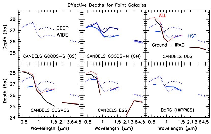
The present determinations of the LFs at -10 make use of all the ultra-deep, wide-area observations obtained as part of the HUDF09+HUDF12, ERS, and CANDELS programs, in conjunction with archival HST observations over these fields. The pure parallel observations from the BoRG/HIPPIES programs are also utilized. A summary of all the deep, wide-area data sets used in the present study is provided in Table 1, along with the redshift ranges of the sources we can select in these data sets. The 5 depths reported in Table 1 are based on the median uncertainties in the total fluxes, as found for the faintest 20% of sources identified as part of a data set (total fluxes are derived using the procedures described in §3.1).
Except for the reduced HST data made publicly available by the BoRG team through the Mikulski archive for Space Telscopes,222http://archive.stsci.edu/prepds/borg/ we rereduced all of these data using the ACS GTO pipeline apsis (Blakeslee et al. 2003) and our WFC3/IR pipeline wfc3red.py (Magee et al. 2011). All fields were reduced and analyzed at a -pixel scale, except the CANDELS UDS/COSMOS/EGS fields (where the pixel scale was ) or BoRG/HIPPIES pure-parallel data sets (where the pixel scale was for the reductions we utilized from Bradley et al. 2012 or where we carried out our own reductions).
XDF: Our deepest search field (reaching to 30 mag at ) is located over the particularly deep 4.7 arcmin2 WFC3/IR pointing defined by the HUDF09 and HUDF12 programs within the HUDF (Beckwith et al. 2006) and takes full advantage of the entire XDF data set (Illingworth et al. 2012) incorporating all ACS and WFC3/IR observations ever taken over the HUDF (reaching 0.2 mag deeper than the original optical HUDF: Beckwith et al. 2006).
HUDF09-Ps Fields: Our second and third deepest search fields are the two deep 4.7 arcmin2 WFC3/IR pointings HUDF09-1 and HUDF09-2 defined by the HUDF09 program (Bouwens et al. 2011). Ultra-deep ACS observations in the bands are available over these fields from the HUDF05, HUDF09, HUDF12, and other programs (Oesch et al. 2007; Bouwens et al. 2011; Ellis et al. 2013). Deep observations are available over the HUDF09-2 field.
CANDELS GOODS-North (GN) + CANDELS GOODS-South (GS) Fields: We also make use of both the deep and intermediate depth observations that exist over the GN and GS fields from the CANDELS program (Grogin et al. 2011). These observations probe 1.5-2.5 mag shallower than our deepest field, the XDF, but cover 30 more area. Deep ACS observations are available over the entire CANDELS-GN, with the deep regions are covered with especially sensitive HST ACS observations (0.5 mag deeper than in the band). Our reductions of these observations include the full set of SNe search and follow-up observations associated with the Riess et al. (2007) programs. Shallow observations in the band (0.3 orbits) are available over most of this area as part of the 3D-HST (Brammer et al. 2012) and AGHAST (Weiner et al. 2014) programs.
ERS Field: Additional constraints on the prevalence of intermediate luminosity -10 galaxies is provided by the ACS and WFC3/IR observations available as part of the 40 arcmin2 Early Release Science observations over GOODS South (Windhorst et al. 2011).
CANDELS-UDS, CANDELS-COSMOS, and CANDELS-EGS Fields: Our strongest constraint on the volume density of the brightest, most luminous galaxies is provided by the 450 arcmin2 search area available over the CANDELS-UDS, CANDELS-EGS, and CANDELS-COSMOS data sets (Grogin et al. 2011). Essentially this entire area is covered by moderately deep WFC3/IR and ACS observations. Deep ground-based observations in both the optical and near-IR from Subaru, CFHT, VLT, and VISTA largely fill out the wavelength coverage available from HST so that it extends from 3500 to 23000, making it possible to select galaxies at , , , , and and also ensure that our selected samples are largely free of contamination by lower redshift interlopers.
BoRG/HIPPIES Fields: The 450 arcmin2 wide-area BoRG/HIPPIES data set (Trenti et al. 2011; Yan et al. 2011; Bradley et al. 2012; Schmidt et al. 2014) effectively doubles the search volume we have available to constrain the prevalence of the rarest, brightest galaxies. The data set features deep observations in and bands (from 25.5 mag to 28.4 mag, 5), as well as observations in two bands blueward of the break, / and /. The BoRG/HIPPIES observations were obtained with HST in parallel with observations from other science programs, providing for excellent controls on large-scale structure uncertainties, due to the many independent areas of the sky probed. Here we make use of the highest-quality search fields (220 arcmin2) taken as part of both the BoRG program and similar data sets. 37 arcmin2 of this search area derives from the HIPPIES program.
With the exception of the BoRG/HIPPIES fields, all of our search fields have deep Spitzer/IRAC observations available that can be used to improve our search for -10 galaxies and better distinguish galaxies from galaxies. Here we make use of the Spitzer/IRAC observations from the GOODS (Dickinson et al. 2004), SEDS (Ashby et al. 2013), IUDF (Labbé et al. 2013), and S-CANDELS (PI Fazio: Oesch et al. 2014) data set over the CANDELS-GN and GS, the IUDF data set over the HUDF/XDF and HUDF09-Ps fields, and the SEDS data set over the CANDELS UDS/COSMOS/EGS fields.
The zeropoints for the ACS and WFC3/IR observations were set according to the STScI zeropoint calculator 333http://www.stsci.edu/hst/acs/analysis/zeropoints/zpt.py and the WFC3/IR data handbook (Dressel et al. 2012). These zeropoints were corrected for foreground galaxy extinction based the Schlafly & Finkbeiner (2011) maps.
Additional details on the data sets or search fields utilized in this study can be found in Appenidx A.
3. Sample Selection
3.1. Photometry
3.1.1 HST Photometry
As in our other recent work, we make use of the SExtractor (Bertin & Arnouts 1996) software in dual-image mode to construct the source catalogs from which we will later select our high-redshift samples. For the detection images, we utilize the square root of image (Szalay et al. 1999: similar to a coadded image) constructed from all available WFC3/IR observations for our , , , and samples, the and -band observations for our samples, and the -band observations for our samples. For the and samples from the XDF data set, we also include the deep -band observations in generating the image.
Color measurements are then made from the observations PSF-matched to the -band in small-scalable apertures derived adopting a Kron (1980) parameter of 1.6. The PSF matching is performed using a kernel derived that when convolved with the tighter PSF matches the -band encircled energy distribution (§2.2 of Bouwens et al. 2014a). We can obtain even higher S/N color measurements at optical wavelengths for sources in our search fields by taking advantage of the narrower PSF of the HST ACS observations. Our procedure is simply (1) to PSF match the ACS observations to the -band and (2) to do the photometry in an aperture that was just 70% the size of that used on the WFC3/IR data. We arrived at the 70% scale factor by comparing the sizes of the scalable Kron-style apertures derived for individual -6 galaxies found in HUDF+GOODS, if PSF-matching is done to the ACS -band data and to the WFC3/IR -band data. Higher S/N optical colors are useful for measuring the amplitude of the Lyman Break in candidate , , and galaxies.
The fluxes measured in the small-scalable apertures were then corrected to total magnitudes in two steps. In the first step, we multiply the small aperture fluxes by the excess light found in a larger scalable aperture (Kron factor of 2.5) relative to smaller scalable aperture. This estimate is made using the square root of image. Second, we correct for the light outside the large scalable aperture and on the wings of the PSF using the standard encircled energy distributions for point sources tabulated in Dressel (2013) or Sirianni et al. (2005). Figure 28 from Appendix H illustrates the typical size of the apertures we use relative to the size of a source. While the source included in Figure 28 is the one of the largest galaxies known (i.e., the largest in the HUDF: Oesch et al. 2010; Ono et al. 2013), this figure illustrates the usefulness of scalable apertures.
3.1.2 Photometry on Ground-Based Imaging Data
In selecting our samples over the wide-area CANDELS-UDS, CANDELS-COSMOS, and CANDELS-EGS fields, we also made use of the deep optical and near-infrared ground-based data available over these same areas of the sky from Subaru, CFHT, VLT, and VISTA (see Appendix A.1). The optical observations reach as deep or deeper than the HST observations and are important for excluding lower redshift contaminants from the -10 samples we construct from these fields. Moderately deep near-IR observations are available in the band and are valuable for discriminating between and candidates in the CANDELS-UDS and CANDELS-COSMOS fields (Appendix A.1).
A significant challenge in extracting photometry for sources from the ground-based data was the broad PSF and therefore the occasional blending of sources with nearby neighbors in the ground-based imaging data. To obtain accurate photometry of sources in the presence of this blending, we made use of Mophongo (Labbé et al. 2006, 2010a, 2010b, 2013) to do photometry on sources in our fields. Since this software has been presented more extensively in other places, we only include a brief description here.
The most important step for doing photometry on faint sources contaminated by light from neighboring sources is the removal of the contaminating flux. This is accomplished by using the deep WFC3/IR -band observations as a template to model the positions and isolated flux profiles of the foreground sources. These flux profiles are then convolved to match the ground-based PSFs and then simultaneously fit to the ground-based imaging data leaving only the fluxes of the sources as unknowns. The best-fit model is then used to subtract the flux from neighboring sources and normal aperture photometry is performed on sources in 1.2′′-diameter apertures. The measured fluxes are then corrected to account for the light on the wings of the ground-based PSFs. Our correction of the measured flux in 1.2′′-diameter apertures to total makes use of the HST template we have for each source (after convolution to match the ground-based PSF). The typical residuals we find in our registration of the ground-based images to the HST observations were 0.04′′. The CANDELS team use a similar approach in deriving photometry for the CANDELS-UDS and CANDELS-GS fields (Galametz et al. 2013; Guo et al. 2013).
3.1.3 IRAC Photometry
Deep Spitzer/IRAC imaging observations available over our search fields provide essential constraints on the shape of source SEDs redward of m for the searches we perform, allowing us to distinguish star-forming galaxies from lower redshift interlopers. See Appendix A of Oesch et al. (2012a) for a discussion of these contaminants.
Our procedure for performing photometry on the deep IRAC observations (Labbé et al. 2006, 2010a, 2010b, 2013) is almost identical to the approach we adopt for the deep ground-based observations (§3.1.2). The positions and morphology of sources in the deep HST observations are used to model and subtract contamination from neighboring sources on candidate galaxies in our search fields. Photometry is then performed on the sources in -diameter apertures, and the measured flux is corrected to total based on the HST template we have for each source convolved to match the Spitzer/IRAC PSF.
To ensure that the photometry we derive is robust, we compared the fluxes we measure for individual sources with results using -diameter apertures and find almost exactly the same measured flux in the mean at both and m ().
| Data Set | |||
|---|---|---|---|
| Sample | XDF, HUDF09-Ps | CANDELS-UDS | |
| CANDELS-GS+GN | ERS, BoRG/HIPPIES$\dagger$$\dagger$The BoRG/HIPPIES data set is only used in searches for galaxies. | COSMOS,EGS | |
| 4 | 1)(1) | 1)(1) | |
| 1.6()+1) | 1.6()+1) | ||
| [not in selection] | [not in selection] | ||
| 5 | 1.2)1.3) | 1.2)1.3) | 1.3)1.25) |
| 0.8(1.2) | 0.8(1.2) | ||
| [ non-detection criterion]aaThe optical non-detection criteria are as follows: [], [], [], [], and []. For our -10 selections, we also require that the optical be less than 4 and 3 in fixed -diameter and 0.2′′-diameter apertures, respectively. We also impose a stricter optical non-detection criterion for the faintest sources in each of our selections (i.e., where the total detection significance as defined by ). These criteria are (), (), (), and (). | [ non-detection criterion]aaThe optical non-detection criteria are as follows: [], [], [], [], and []. For our -10 selections, we also require that the optical be less than 4 and 3 in fixed -diameter and 0.2′′-diameter apertures, respectively. We also impose a stricter optical non-detection criterion for the faintest sources in each of our selections (i.e., where the total detection significance as defined by ). These criteria are (), (), (), and (). | ||
| [not in selection] | [not in selection] | (5.5)())ccWhile we select sources to 26.7 mag, we only include sources brightward of 26.5 mag in our LF determinations. | |
| [other LBGs with 5.5]bbWe also include sources in our , , , and selections, respectively, if they satisfy any of our , , and -8 LBG criteria and the photometric redshifts we estimate for the sources are , , , and , respectively, with a total measured magnitude of , , , and . See §3.2.3. | |||
| 6 | 1.0)(1.0) | 1.0)(1.0) | (0.8)0.4) |
| 0.78()1.0) | 0.6()1.0) | (2()0.8) | |
| [ non-detection criterion]aaThe optical non-detection criteria are as follows: [], [], [], [], and []. For our -10 selections, we also require that the optical be less than 4 and 3 in fixed -diameter and 0.2′′-diameter apertures, respectively. We also impose a stricter optical non-detection criterion for the faintest sources in each of our selections (i.e., where the total detection significance as defined by ). These criteria are (), (), (), and (). | [ non-detection criterion]aaThe optical non-detection criteria are as follows: [], [], [], [], and []. For our -10 selections, we also require that the optical be less than 4 and 3 in fixed -diameter and 0.2′′-diameter apertures, respectively. We also impose a stricter optical non-detection criterion for the faintest sources in each of our selections (i.e., where the total detection significance as defined by ). These criteria are (), (), (), and (). | 2.5) | |
| [not in selection] | [not in selection] | (6.3)())ccWhile we select sources to 26.7 mag, we only include sources brightward of 26.5 mag in our LF determinations. | |
| [other LBGs with 6.3]bbWe also include sources in our , , , and selections, respectively, if they satisfy any of our , , and -8 LBG criteria and the photometric redshifts we estimate for the sources are , , , and , respectively, with a total measured magnitude of , , , and . See §3.2.3. | |||
| 7 | 0.7)0.45) | 1.3) 0.5) | 2.2)0.4) |
| 0.8()+0.7) | 0.8()0.7) | 2()2.2) | |
| 1.0)1.5)) | 1.0)1.5)) | 2.5) | |
| [ non-detection criterion]aaThe optical non-detection criteria are as follows: [], [], [], [], and []. For our -10 selections, we also require that the optical be less than 4 and 3 in fixed -diameter and 0.2′′-diameter apertures, respectively. We also impose a stricter optical non-detection criterion for the faintest sources in each of our selections (i.e., where the total detection significance as defined by ). These criteria are (), (), (), and (). | [ non-detection criterion]aaThe optical non-detection criteria are as follows: [], [], [], [], and []. For our -10 selections, we also require that the optical be less than 4 and 3 in fixed -diameter and 0.2′′-diameter apertures, respectively. We also impose a stricter optical non-detection criterion for the faintest sources in each of our selections (i.e., where the total detection significance as defined by ). These criteria are (), (), (), and (). | ||
| [not in selection] | [not in selection] | (26.7)ccWhile we select sources to 26.7 mag, we only include sources brightward of 26.5 mag in our LF determinations. | |
| [other LBGs with 7.3]bbWe also include sources in our , , , and selections, respectively, if they satisfy any of our , , and -8 LBG criteria and the photometric redshifts we estimate for the sources are , , , and , respectively, with a total measured magnitude of , , , and . See §3.2.3. | |||
| 8 | (0.45)0.5) | 1.3)0.5) | 2.2)0.4) |
| 0.75()0.525) | 0.75()1.3) | 2()2.2) | |
| [ non-detection criterion]aaThe optical non-detection criteria are as follows: [], [], [], [], and []. For our -10 selections, we also require that the optical be less than 4 and 3 in fixed -diameter and 0.2′′-diameter apertures, respectively. We also impose a stricter optical non-detection criterion for the faintest sources in each of our selections (i.e., where the total detection significance as defined by ). These criteria are (), (), (), and (). | [ non-detection criterion]a,da,dfootnotemark: | 2.5) | |
| (7.39.0)26.7)ccWhile we select sources to 26.7 mag, we only include sources brightward of 26.5 mag in our LF determinations. | |||
| [other LBGs with 9.0]bbWe also include sources in our , , , and selections, respectively, if they satisfy any of our , , and -8 LBG criteria and the photometric redshifts we estimate for the sources are , , , and , respectively, with a total measured magnitude of , , , and . See §3.2.3. | |||
| 10 | 1.2) | (1.2) | (1.2) |
| [3.6]1.4) | ((1.4) | (([3.6]1.4) | |
| 2)) | 2)) | 2)) | |
| [ non-detection criterion]aaThe optical non-detection criteria are as follows: [], [], [], [], and []. For our -10 selections, we also require that the optical be less than 4 and 3 in fixed -diameter and 0.2′′-diameter apertures, respectively. We also impose a stricter optical non-detection criterion for the faintest sources in each of our selections (i.e., where the total detection significance as defined by ). These criteria are (), (), (), and (). | [ non-detection criterion]aaThe optical non-detection criteria are as follows: [], [], [], [], and []. For our -10 selections, we also require that the optical be less than 4 and 3 in fixed -diameter and 0.2′′-diameter apertures, respectively. We also impose a stricter optical non-detection criterion for the faintest sources in each of our selections (i.e., where the total detection significance as defined by ). These criteria are (), (), (), and (). | 2.5) | |
| (2) | |||
| All | [Stellarity Criterion]eeWe require that the measured stellarity of sources (as measured in the detection image) be less than 0.9 to exclude stars from our samples (0 = extended source and 1 = point source). We also exclude particularly compact sources, with detection-image stellarities less than 0.9 if its HST + ground-based + Spitzer photometry is significantly better fit with a stellar SED than a galaxy () and the measured stellarity in either the or band is at least 0.8. The stellarity requirement is only imposed within 1 magnitude of the detection limit of the sample, i.e., 26.5 mag for the CANDELS/Wide data sets, 27.0 mag for the CANDELS/DEEP data sets, 28.0 mag for the HUDF09-1+HUDF09-2 data sets, and 28.5 mag for the XDF data set. | [Stellarity Criterion]eeWe require that the measured stellarity of sources (as measured in the detection image) be less than 0.9 to exclude stars from our samples (0 = extended source and 1 = point source). We also exclude particularly compact sources, with detection-image stellarities less than 0.9 if its HST + ground-based + Spitzer photometry is significantly better fit with a stellar SED than a galaxy () and the measured stellarity in either the or band is at least 0.8. The stellarity requirement is only imposed within 1 magnitude of the detection limit of the sample, i.e., 26.5 mag for the CANDELS/Wide data sets, 27.0 mag for the CANDELS/DEEP data sets, 28.0 mag for the HUDF09-1+HUDF09-2 data sets, and 28.5 mag for the XDF data set. | [Stellarity Criterion]eeWe require that the measured stellarity of sources (as measured in the detection image) be less than 0.9 to exclude stars from our samples (0 = extended source and 1 = point source). We also exclude particularly compact sources, with detection-image stellarities less than 0.9 if its HST + ground-based + Spitzer photometry is significantly better fit with a stellar SED than a galaxy () and the measured stellarity in either the or band is at least 0.8. The stellarity requirement is only imposed within 1 magnitude of the detection limit of the sample, i.e., 26.5 mag for the CANDELS/Wide data sets, 27.0 mag for the CANDELS/DEEP data sets, 28.0 mag for the HUDF09-1+HUDF09-2 data sets, and 28.5 mag for the XDF data set. |
| ffEven more stringent requirements are made on the detection significance of sources in data sets shallower than the XDF. Candidates are required to have a total signal-to-noise in the , , , and bands of 5.5 in the HUDF09-Ps and CANDELS data set, and 6.0 in the BoRG/HIPPIES data set. For and selections, only the and fluxes, respectively, are used in assessing the detection significance of candidate sources. candidates over the CANDELS-UDS/COSMOS/EGS fields are required to have a root-mean square S/N of 2.0 in the Spitzer/IRAC m and m imaging to ensure they are real. | ffEven more stringent requirements are made on the detection significance of sources in data sets shallower than the XDF. Candidates are required to have a total signal-to-noise in the , , , and bands of 5.5 in the HUDF09-Ps and CANDELS data set, and 6.0 in the BoRG/HIPPIES data set. For and selections, only the and fluxes, respectively, are used in assessing the detection significance of candidate sources. candidates over the CANDELS-UDS/COSMOS/EGS fields are required to have a root-mean square S/N of 2.0 in the Spitzer/IRAC m and m imaging to ensure they are real. | ffEven more stringent requirements are made on the detection significance of sources in data sets shallower than the XDF. Candidates are required to have a total signal-to-noise in the , , , and bands of 5.5 in the HUDF09-Ps and CANDELS data set, and 6.0 in the BoRG/HIPPIES data set. For and selections, only the and fluxes, respectively, are used in assessing the detection significance of candidate sources. candidates over the CANDELS-UDS/COSMOS/EGS fields are required to have a root-mean square S/N of 2.0 in the Spitzer/IRAC m and m imaging to ensure they are real. | |
3.2. Source Selection
3.2.1 Lyman-Break Selection Criteria
As in previous work, we construct the bulk of our high-redshift samples using two color Lyman-break-like criteria. Substantial spectroscopic follow-up work has shown that this approach is quite effective at identifying large samples of star-forming galaxies at (Steidel et al. 1999; Bunker et al. 2003; Dow-Hygelund et al. 2007; Popesso et al. 2009; Vanzella et al. 2009; Stark et al. 2010).
Lyman-break samples typically take advantage of three pieces of information in identifying probable sources at high redshift: (1) color information from two adjacent passbands necessary to locate the position and measure the amplitude of the Lyman break, (2) color information redward of the break needed to define the intrinsic color of the source (thereby distinguishing the selected high-redshift sources from intrinsically-red galaxies), and (3) evidence that sources show essentially no flux blueward of the spectral break.
Our selection is constructed to take advantage of all three pieces of information and to do so in a suitably optimal manner, within the context of simple color criteria. The most noteworthy gains can be achieved by taking advantage of the additional wavelength leverage provided by the deep near-IR and mid-IR observations for constraining the intrinsic colors of candidate sources. This allows us to go beyond what is possible from the Lyman-break-like selection utilized in Giavalisco et al. (2004b) and Bouwens et al. (2007). Obviously, the color which provides us with the most significant leverage in probing the intrinsic colors of the sources are those we would use to provide optimal measurements of the spectral slope (e.g., we use the same color below in constructing our color criterion for the selection as would be optimal for deriving for galaxies: Bouwens et al. 2012; Bouwens et al. 2014a).
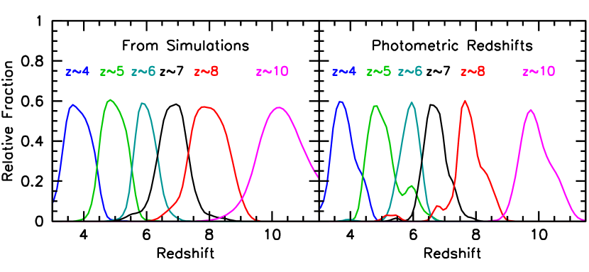
While one could consider selecting -10 samples based on the best-fit photometric redshift or redshift likelihood contours (e.g., McLure et al. 2010; Finkelstein et al. 2012; Bradley et al. 2014: see Figure 1 [right]), Lyman-break selection procedures can be simpler to apply and offer a slight advantage in terms of operational transparency. This makes our selection procedure easier to reproduce by both theorists and observers, as follow-up studies by Shimizu et al. (2013), Lorenzoni et al. (2013), and Schenker et al. (2013) utilizing our color criteria all illustrate.
Despite the present procedural choice, photometric redshift techniques also work quite well, particularly when used with a well-calibrated prior or as refinements to the redshift estimate, as direct comparisons between LF determinations conducted using Lyman-break-like selection criteria (e.g., Schenker et al. 2013) and photometric-redshift selection criteria (e.g., McLure et al. 2013) illustrate. Indeed, we will be utilizing photometric redshift techniques in §3.2 to redistribute sources across our CANDELS-UDS/COSMOS/EGS , , , and samples based on our best estimate redshifts from the HST + ground-based + Spitzer/IRAC observations.
3.2.2 XDF, HUDF09-1, HUDF09-2, CANDELS-GS, CANDELS-GN, ERS, BoRG/HIPPIES
In this section, we describe the selection criteria we employ for data sets with deep observations in the -band with HST, i.e., the XDF, HUDF09-1, HUDF09-2, CANDELS-GS, CANDELS-GN, ERS, and the BoRG/HIPPIES fields.
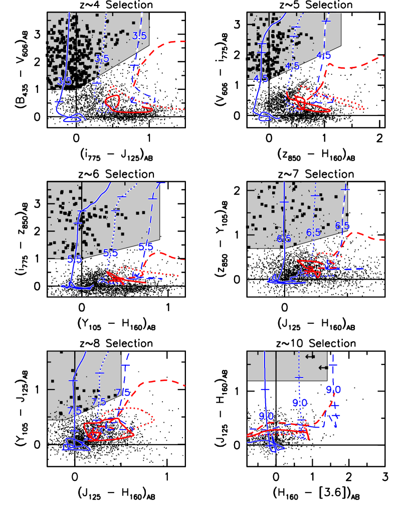
We have constructed two-colour selection criteria so that the lower-redshift boundary is approximately the same for sources independent of their spectral slope. For those areas where the -band observations are available in the -band filter, we use one set of criteria, while for those areas where the is available, we employ an alternate set of selection criteria. The specific color criteria we have developed are presented in Table 2.
The new color criteria we have developed are not directly comparable to those previously developed to work with optical/ACS observations (Giavalisco et al. 2004b; Bouwens et al. 2007), though we remark that the , , color criteria that we utilize (to identify the existence of a Lyman-break) are almost identical to previous criteria. Our color criteria are most similar in spirit to the criteria previously developed by Castellano et al. (2012), though Castellano et al. (2012) use a color to quantify the color of galaxies redward of the break rather than an color. The advantage of using the colors over the colors is the cleaner measurement it provides of the slope of the -continuum for candidate galaxies (though the wavelength leverage it provides is less).
The and color criteria we utilize here are very similar to the criteria we had previously applied in Bouwens et al. (2011b) to the HUDF and ERS data sets. See Figures 2 and 3 and Figures 6 and 7 from Bouwens et al. (2011b). The selection criteria we employ over the ERS+BoRG+HIPPIES fields utilizes a less stringent cut than the cut utilized in the standard BoRG search (e.g., Bradley et al. 2012), making our selection slightly more susceptible to contamination by low-mass stars. However, such sources should be largely excluded by stellarity criterion we discuss below (see also §3.5.5).
Finally, our selection criteria are identical to those previously presented by Bouwens et al. (2011), Oesch et al. (2012a), and Oesch et al. (2014).
In applying these criteria, we set the flux in the dropout band to be equal to the upper limit in cases of a non-detection.
In isolation, the color criteria we present in Table 2 would allow for the selection of sources at least one unit higher in redshift than our desired high-redshift boundaries for these selections (e.g., our selection criteria could allow us to select sources from to ). Fortunately, we can impose a high-redshift boundary for each of our selections by explicitly requiring that sources not satisfy the selection criteria for the sample just above it in redshift. This ensures that our selections are both essentially complete and disjoint from one another.
To keep contamination from lower redshift sources to a minimum, we require that sources in our and selections be undetected () in -band imaging data for our fields, if it is available. For our selections, we require the color to be redder than 2.6 or for sources to be undetected () in the -band imaging data (similar to Bouwens et al. 2006). For our -10 selections, we calculate an optical “” for each candidate source (Bouwens et al. 2011), as where is the flux in band in a consistent aperture, is the uncertainty in this flux, and SGN() is equal to 1 if and if . The flux measurements (where available) were used in calculating for our selections, while the and observations were used in computing for our and selections, respectively. is computed on the basis of the flux measurements in small-scalable apertures; any candidate with a measured in excess of 3 is excluded from our selections.
For our highest redshift selections, i.e., -10, we also computed a for sources in 0.35′′-diameter apertures and especially small -diameter apertures (before PSF smoothing to preserve S/N) and required sources to be less than 3 and 4 respectively. An even lower threshold of 2 for was used in selecting -8 sources over the HUDF09-1 field, due to the lack of -band observations over that field. Finally, for the faintest -8 candidates in each of our selections with a coadded significance of the detections in the , , , , and bands less than 8 (i.e., ), we used the even more stricter requirements on the flux in the optical bands listed in footnote a of Table 2.
For our deepest field the XDF, sources are required to be detected at in a stack of all the HST observations redward of the break (in a fixed 0.36′′-diameter aperture). This is to ensure source reality. For sources over the deep HUDF09-1 and HUDF09-2 fields and the wider-area CANDELS and ERS fields, we require sources be detected at . For sources over the BoRG/HIPPIES fields, we require sources to be detected at . Our use of more stringent criteria for our shallower fields is quite reasonable, given the much smaller number of exposures in these data and therefore noise that is less Gaussian in its characteristics (e.g., see Schmidt et al. 2014).444While we could increase the total number of sources in our selections somewhat by searching for sources at lower significance levels, these sources are not of substantial value for current LF determinations, given the considerable uncertainties in correcting for both the incompleteness and contamination expected for such samples.
| ID | R.A. | Dec | SampleaaThe mean redshift of the sample in which the source was included for the purposes of deriving LFs. | Data SetbbThe data set from which the source was selected: 1 = HUDF/XDF, 2 = HUDF09-1, 3 = HUDF09-2, 4 = ERS, 5 = CANDELS-GS, 6 = CANDELS-GN, 7 = CANDELS-UDS, 8 = CANDELS-COSMOS, 9 = CANDELS-EGS, and 10 = BoRG/HIPPIES or other pure-parallel programs. | c,dc,dfootnotemark: | |
|---|---|---|---|---|---|---|
| XDFB-2384848214 | 03:32:38.49 | 27:48:21.4 | 27.77 | 4 | 1 | 3.49 |
| XDFB-2384248186 | 03:32:38.42 | 27:48:18.7 | 29.18 | 4 | 1 | 3.82 |
| XDFB-2376648168 | 03:32:37.66 | 27:48:16.9 | 28.61 | 4 | 1 | 4.01 |
| XDFB-2385948162 | 03:32:38.60 | 27:48:16.2 | 28.04 | 4 | 1 | 4.16 |
| XDFB-2382548139 | 03:32:38.26 | 27:48:13.9 | 28.18 | 4 | 1 | 4.37 |
| XDFB-2394448134 | 03:32:39.45 | 27:48:13.4 | 26.40 | 4 | 1 | 3.58 |
| XDFB-2381448127 | 03:32:38.14 | 27:48:12.7 | 28.58 | 4 | 1 | 3.68 |
| XDFB-2390248129 | 03:32:39.03 | 27:48:13.0 | 27.99 | 4 | 1 | 3.91 |
| XDFB-2379348121 | 03:32:37.93 | 27:48:12.1 | 27.45 | 4 | 1 | 4.11 |
| XDFB-2378848108 | 03:32:37.88 | 27:48:10.9 | 30.13 | 4 | 1 | 3.72 |
For sources that are at least 1 magnitude brightward of the nominal detection limit for our samples (i.e., 26.5 mag for the CANDELS/Wide data sets, 27.0 mag for the CANDELS/DEEP data sets, 28.0 mag for the HUDF09-1+HUDF09-2 data sets, and 28.5 mag for the XDF data set), the SExtractor stellarity parameter for sources (from SExtractor detection image) is required to be less than 0.9 (where 0 corresponds to very extended sources and 1 corresponds to point sources). We also exclude particularly compact sources, with measured stellarities (from detection image) greater than 0.5 if its HST photometry was significantly better fit to a stellar SED than a galaxy () and if the measured stellarity in either the or image is greater than 0.8. The templates we use for our stellar SED fits are from the SpeX prism library of low-mass stars (Burgasser et al. 2004) extended to m using the derived spectral types and the known -[3.6] or -[4.5] colors of these spectral types (Patten et al. 2006; Kirkpatrick et al. 2011).
Finally, a careful visual inspection was performed on all of the candidate -10 galaxies that otherwise satisfy our selection criteria to exclude obvious artifacts (e.g., diffraction spikes, spurious “sources” on the wings of ellipticals) or any sources that seemed likely to be associated with bright foreground sources.555We note the exclusion of two bright () candidates identified over the BoRG/HIPPIES data set from our selection as a result of these concerns (at positions 22:02:50.00, 18:51:00.2 and 08:35:13.13, 24:55:38.1). We also verified that none of the sources in our selection were previously included in the catalogs of candidate low-mass stars from Holwerda et al. (2014a) or were associated with SNe identified during the CANDELS observations (Rodney et al. 2014).
3.2.3 CANDELS-UDS, CANDELS-COSMOS, CANDELS-EGS Fields
Because of the lack of deep HST imaging in , , or /-band over the CANDELS-UDS, CANDELS-COSMOS, and CANDELS-EGS fields (Table 1 and Figure 2), it is not possible to select -8 galaxies over those fields using the same color criteria as we utilized over our primary search fields (i.e., the XDF, CANDELS-GN, and CANDELS-GS).
Our procedure for selecting our samples of , , and galaxies over these is therefore more involved and makes significant use of the ground-based observations. We describe our procedure in the paragraphs that follow. The first step was to identify all those sources that plausibly corresponded to star-forming galaxies at -8 through the systematic selection of Lyman-break-like galaxies at , , and -8. The criteria we used to do this preselection is presented in Appendix B.
In the second step, we obtained photometry on each of these sources in deep ground-based Subaru+CFHT+VLT+VISTA + Spitzer/IRAC observations that are available over our search fields. We then used the EAZY photometric redshift code (Brammer et al. 2008) to estimate redshifts for all the sources. The photometry utilized in deriving the photometric redshifts included flux measurements from the HST + Subaru-SuprimeCam + CFHT/Megacam + UltraVISTA data sets for the CANDELS COSMOS field, HST + Subaru-SuprimeCam + CFHT/Megacam + UKIRT/WFCAM + VLT/HAWKI/HUGS data sets for the CANDELS UDS field, and the HST + CFHT/Megacam + CFHT/WIRCam + Spitzer/IRAC 3.6m+4.5m data sets for the CANDELS EGS field. No consideration of the Spitzer/IRAC photometry is made for sources over the CANDELS-UDS and CANDELS-COSMOS fields due to the availability of deep -band observations to distinguish sources from sources.666In addition, this exclusion of the Spitzer/IRAC data in this selection allowed us to avoid introducing any coupling between redshift and the Spitzer/IRAC properties of our sources for future analyses.
Sources with photometric redshifts in the range -5.5, -6.3, -7.3, and -9.0 were tentatively assigned to our , , , and selections, respectively. These redshift ranges were chosen to ensure a good match with the mean redshifts for the color selections defined in §3.2.2. Our photometric redshift fitting is conducted using the EAZY_v1.0 template set supplemented by SED templates from the Galaxy Evolutionary Synthesis Models (GALEV: Kotulla et al. 2009). Nebular continuum and emission lines were added to the later templates using the Anders & Fritze-v. Alvensleben (2003) prescription, a metallicity, and a rest-frame EW for H of 1300Å.777While the rest-frame EW we assume for for our adapted GALEV templates is larger than the 500-600 EW typical for many galaxies (e.g., Shim et al. 2011; Stark et al. 2013), such templates have been included to give the EAZY photometric code (which can consider arbitrary linear combinations of SED templates) the flexibility to accurately model the SEDs of galaxies with very strong line emission. These templates effectively counterbalance our use of the standard template set, where the impact of line emission is minimal.
We only included galaxies in our , , and samples brightward of mag (-7) and mag () in our samples as a whole. However, only sources brightward of 26.5 mag are used in our LF determinations (§4). This was to ensure good redshift separation, given the limited depth of the -band observations and ground-based and -band observations (Figure 2). As we demonstrate with the simulations in §4.1 (illustrated in Figure 4), we can effectively split sources into different redshift subsamples to 26.5 mag.
To ensure that each of these candidate -8 galaxies was robust, we required that each of these sources show 2.5 detection blueward of the break. To this end, inverse-variance-weighted fluxes were derived for each source blueward of the Lyman break. Included in the inverse-variance-weighted measurements for the samples in brackets below were the CFHT Megacam and Subaru Suprime-Cam [CANDELS-UDS ], CFHT and Subaru [CANDELS-UDS ], CFHT and Subaru [CANDELS-UDS ], CFHT and Subaru [CANDELS-UDS ], CFHT MegaCam [COSMOS ], Subaru and CFHT [COSMOS ], Subaru and CFHT [COSMOS ], Subaru and CFHT [COSMOS ], CFHT [EGS ], CFHT [EGS ], CFHT [EGS ], and CFHT [EGS ] flux measurements, respectively. We also excluded candidate , , and galaxies from our selection where flux in the HST , , and bands was greater than 1.5. Exclusion of sources with detections blueward of the break only had a modest effect on the size of the , , , and samples we derived from the wide-area CANDELS fields (removing 2%, 7%, 8%, and 21% of the sources from the , , , and samples, respectively).888We also note the exclusion of a candidate at 10:00:13.93, 2:22:14.9, due to its showing far too much flux in the ground-based and -band data (3- discrepancy in both cases) to be a robust candidate.
We used a similar strategy for excluding stars from our CANDELS-UDS, COSMOS, and EGS fields, as what we utilize for selections over the XDF, HUDF09-Ps, ERS, CANDELS-GN+GS, and the BoRG/HIPPIES fields (§3.2.2). The only procedural difference with the present fields is that we also make use of the ground-based + Spitzer/IRAC photometry we obtain for sources in ascertaining whether their SEDs are more consistent with that of a star or a -8 galaxy. Using simulations where we added point-like sources to the real data with input fluxes taken from random stars in the SpeX prism library of late-type stars (Burgasser et al. 2004), we found that our schema was successful at excluding 97%, 97%, and 94% of -26.5 stars from our selection over the CANDELS-UDS, CANDELS-COSMOS, and CANDELS-EGS fields, respectively (with late L and early T type stars being the most challenging to exclude).
As a check on the fidelity of our -8 samples, we also derived fluxes for sources in our samples in larger -diameter apertures than we used for our fiducial selection. Coadding the fluxes of sources blueward of the break while weighting by the inverse variance, we found that 94% of the sources in our samples remain undetected at even in larger -diameter aperture. To interpret these findings, we repeated this experiment on the mock images we created in §4.1 and found similar incompleteness levels, strongly arguing that the slight detection rate we found for our -8 samples in the larger apertures could be explained as resulting from noise and imperfectly subtracted nearby neighbors.999To check the robustness of our flux measurements in the -band to the size of the high-redshift sources, we derived -band fluxes for the brightest sources in -diameter apertures for comparison with our smaller-aperture measurements. Encouragingly enough, the -band fluxes we recovered were completely consistent (35% lower) using the wider apertures as using our fiducial -diameter apertures. This is not surprising, since mophongo accounts for the expected profile of the source in the ground-based observations in correcting the aperture measurements to total.
We further stacked the optical -band observations (blueward of the break for galaxies) for all 107 and candidates from the wide-area fields and found no detection (). Similar stack results in the band for our CANDELS-UDS/COSMOS/EGS samples yielded no detection.
Our selection of galaxies over these fields is very similar to our selection of galaxies from HST fields with -band imaging (§3.2.2). Again, we require that sources satisfy a color cut, show a detection in the -band, be undetected in a stack of the optical/ACS data (), and also be detected at in the band. However, we also require sources remain undetected () in whatever -band observations were available over our search fields (i.e., from HAWK-I and VISTA over the CANDELS-UDS and CANDELS-COSMOS fields, respectively), that sources also remain undetected () in a stack of the optical ground-based Subaru+CFHT observations available over each field, and that sources be detected at in the available m+m IRAC imaging over the CANDELS fields from the SEDS program (Ashby et al. 2013) to ensure source reality.
| Area | |||||||
|---|---|---|---|---|---|---|---|
| Field | (arcmin2) | # | # | # | # | # | # |
| HUDF/XDF | 4.7 | 357 | 153 | 97 | 57 | 30 | 2 |
| HUDF09-1 | 4.7 | — | 91 | 38 | 22 | 18 | 0 |
| HUDF09-2 | 4.7 | 147 | 77 | 32 | 23 | 17 | 0 |
| CANDELS-GS-DEEP | 64.5 | 1590 | 471 | 198 | 77 | 27 | 1 |
| CANDELS-GS-WIDE | 34.2 | 451 | 117 | 43 | 5 | 3 | 0 |
| ERS | 40.5 | 815 | 205 | 61 | 47 | 6 | 0 |
| CANDELS-GN-DEEP | 68.3 | 1628 | 634 | 188 | 134 | 51 | 2 |
| CANDELS-GN-WIDE | 65.4 | 871 | 282 | 69 | 39 | 18 | 1 |
| CANDELS-UDS | 151.2 | — | 270 | 33 | 18 | 6 | 0 |
| CANDELS-COSMOS | 151.9 | — | 320 | 48 | 15 | 9 | 0 |
| CANDELS-EGS | 150.7 | — | 381 | 50 | 44 | 9 | 0 |
| BORG/HIPPIES | 218.3 | — | — | — | — | 23 | 0 |
| Total | 959.1 | 5859 | 3001 | 857 | 481 | 217 | 6 |
3.3. Selection Results
Applying the selection criteria from §3.2 to XDF, HUDF09-Ps, ERS, BoRG/HIPPIES, and CANDELS data sets results in 5859, 3001, 857, 481, 217, and 6 sources in our , , , , , and samples. Our total -10 sample includes 10400 sources. The individual number of high-redshift candidates in each field is provided in Table 4.
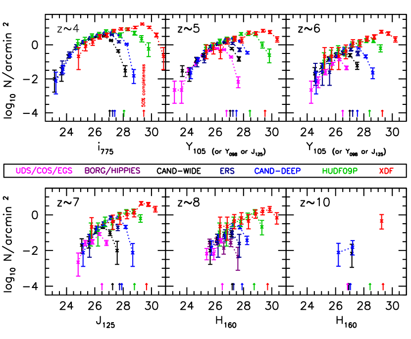
The surface density of galaxies we find in our different redshift samples is presented in Figure 5 as a function of magnitude. While it is clear that some field-to-field variations exist in the surface density of galaxies in our different samples (e.g., galaxies in the HUDF seem to be underdense relative to our other search fields), overall the surface density of galaxies as a function of magnitude is fairly similar for each of our search fields, over magnitude ranges where our search is largely complete. We discuss field-to-field variations in detail in §4.5. In Table 8 from Appendix C, we tabulate the average surface density of galaxies in our different samples as a function of magnitude.
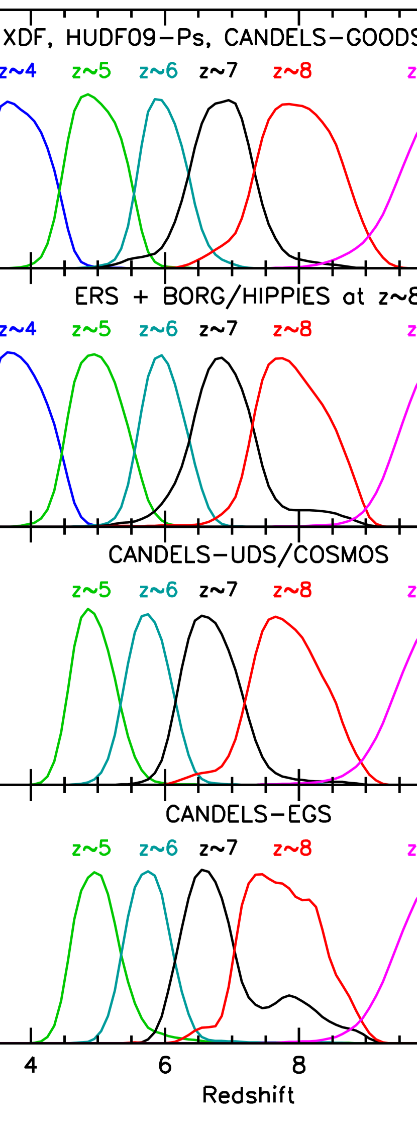
Our best estimate of the approximate redshift distribution for our different high-redshift samples is shown in the left panel of Figure 1 and is based on the simulations we describe in §4.1 for the XDF, HUDF09-1, and HUDF09-2 fields. The mean redshift for galaxies in our , , , , and samples is 3.8, 4.9, 5.9, 6.8, and 7.9. From these simulations, it is clear that our selection criteria are quite effective in dividing high-redshift galaxies into discrete redshift slices. In the right panel of Figure 1, we also present the redshift distributions we derive for our XDF, HUDF09-1, and HUDF09-2 samples using the photometric redshift code EAZY (Brammer et al. 2008). Photometric redshifts are estimated based on the HST photometry (for our -8 samples) and HST+Spitzer photometry (for our sample). As is clear from the figure, our simple color-color selections result in essentially the same subdivision of sources by redshift, as one would find if one relied on a photometric redshift code to do the selection.
We include our complete , , , , , and catalogs in Table 3, with coordinates and rest-frame luminosities. We have also provided our best estimate redshifts for each of the -8 candidates we identified over the CANDELS-UDS/COSMOS/EGS fields. Photometric redshift estimates are also provided for -10 candidates over XDF, HUDF09-Ps, ERS, CANDELS-GS/GN, and BoRG/HIPPIES by applying the photometric redshift software EAZY (Brammer et al. 2008) and the template set from §3.3.2 to the HST photometry we have available for these candidates. To improve the accuracy of the photometric redshift estimates for our CANDELS-GN+GS+ERS samples (where the lack of photometric constraints blueward of the band can impact the results), we have also incorporated the -band photometry of these candidates from KPNO (Capak et al 2004) and VLT/VIMOS (Nonino et al. 2009) using mophongo in fixed 1.2′′-diameter apertures.
3.4. Comparisons with Previous -10 Samples
The present compilation of -10 galaxy candidates from the XDF, HUDF09-1, HUDF09-2, the ERS, and the five CANDELS fields contains 10400 -10 candidates and is the largest such compilation obtained to the present based on HST observations. Previously, the largest such samples of galaxies found in HST observations were reported in Bouwens et al. (2007: 6714 sources over the range -6) and Bouwens et al. (2014a: 4004 sources over the range -8).
A substantial fraction (30-70%) of the sources from the current catalogs appeared in previous wide-area selections. 2331, 586, and 206 of the , , and candidates (44%, 34%, and 37% of this sample, respectively) from our wide-area CANDELS+ERS selections were previously reported by Bouwens et al. (2007). For -8 selections over the CANDELS-GS, 59 and 28 of the and candidates (19% and 27% of this sample, respectively), were previously reported by Bouwens et al. (2011), Oesch et al. (2012), Grazian et al. (2012), Yan et al. (2012), Lorenzoni et al. (2013), Schenker et al. (2013), and McLure et al. (2013). 22 of the present candidates over the CANDELS-UDS and CANDELS-EGS fields (35% of our sample) previously appeared in the Grazian et al. (2012) or McLure et al. (2013). The brightest candidate we find in the CANDELS-UDS field is the well-known “Himiko” Ly-emitting galaxy previously reported by Ouchi et al. (2009a). The brightest 3 and brightest 2 galaxies from our CANDELS-COSMOS catalog were previously identified by Willott et al. (2013) and Bowler et al. (2014), respectively.
11 of the 23 candidates we identified over the BoRG/HIPPIES fields and similar data sets (i.e., 48%) were previously identified as candidates by Bradley et al. (2012), McLure et al. (2013), and Schmidt et al. (2014). The reason our catalogs include many candidates not included in the Bradley et al. (2012) and Schmidt et al. (2014) compilation is our use of one additional data set not previously considered (i.e., a parallel field outside of Abell 1689) and our selecting sources with slightly weaker breaks and slightly redder colors (consistent with our selection from the ERS data set). While excluding these sources may allow Bradley et al. (2012) and Schmidt et al. (2014) to identify a marginally cleaner selection of galaxies, Bradley et al. (2012) and Schmidt et al. (2014) potentially miss a modest fraction of the luminous galaxies over the BoRG/HIPPIES search fields (i.e., those having significantly redder colors than would be selected by their criteria).101010A good fraction of the brightest -8 sources would have ’s of (Bouwens et al. 2012; Finkelstein et al. 2012; Willott et al. 2013; Bouwens et al. 2014a), which is redder than would be selected by the Bradley et al. (2012) and Schmidt et al. (2014) criteria. Our selection criteria are effective in identifying galaxies with ’s as blue as 0 (corresponding to colors of 0.5).
For fainter -8 samples from the XDF, HUDF09-1, and HUDF09-2 data sets, our samples again show very good overlap. 209, 139, 92, 75, and 45 of the present sample of , , , , and candidates (41%, 43%, 55%, 72%, and 71% of this sample, respectively) were previously reported by Bouwens et al. (2007), Wilkins et al. (2010), Bouwens et al. (2011), Schenker et al. (2013), and McLure et al. (2013). The reason the current selection contains many sources that were not previously found by Bouwens et al. (2007) is due to our ability to probe to greater depths with WFC3/IR than was possible using the HST/ACS optical camera alone and deeper optical observations now available over the XDF/HUDF and HUDF09-2 fields.
The present sample is thus far the most comprehensive in the literature, including some 698 -8 high-quality candidates based on all search fields.
The present sample contains 6 candidates in total and is almost identical to the Oesch et al. (2014) sample, with 1 candidate over the CANDELS-GS field, 3 candidates over the CANDELS-GN field, and 2 candidates over the XDF data set. One of the 6 candidates from the present sample (XDFyj-40248004) was classified as a candidate in Oesch et al. (2013b). The earlier analyses of Ellis et al. (2013) and Oesch et al. (2013b) had only identified one plausible candidate each,111111Oesch et al. (2013b) demonstrated that one of the two candidates reported by Ellis et al. (2013), i.e., HUDF12-4106-7304, is significantly boosted by a diffraction spike and therefore cannot be considered a reliable candidate. while McLure et al. (2013) did not identify any candidates over our search fields.121212While we would have expected McLure et al. (2013) to have identified both of the plausible -10 candidates Oesch et al. (2014) identified over the CANDELS-GS field, the apertures McLure et al. (2013) used on these sources could have easily included optical flux from neighboring sources (as occurred for Oesch et al. 2012a: see Appendix A of Oesch et al. 2014), resulting in McLure et al. (2013) excluding them from their “robust” candidate list.
3.5. Contamination
We carefully considered many possible sources of contamination for our -10 samples. Potential contaminants include stellar sources, time-variable events like supernovae, spurious sources, extreme emission-line galaxies, and photometric scatter. We discuss possible contamination by each of these sources in the subsections that follow.
3.5.1 Stars
One potential contaminant for our samples is from stars in our own galaxy, particularly very low-mass stars. It is now well established that low-mass stars have very similar colors to those of -7 galaxies and hence could be a meaningful contaminant, if one does not have information on the spatial profile of galaxies (Stanway et al. 2003; Bouwens et al. 2006; Ouchi et al. 2009b; Tilvi et al. 2013). Since we explicitly exclude points sources from our selection, i.e., sources with a SExtractor stellarity index greater than 0.9 (where 0 and 1 correspond to an extended and point source, respectively) and an apparent magnitude at least one magnitude brighter than the limit, we would expect contamination from stellar sources to be somewhat limited. Bouwens et al. 2006 found the SExtractor stellarity parameter to be very effective in distinguishing point sources from extended sources, for sources with sufficiently high signal-to-noise (i.e., 10).
Near the detection limit of our samples, a small level of contamination is expected, given that we no longer attempt to remove point sources at such low S/Ns. We estimated this contamination by deriving the number counts for all point-like sources in the CANDELS fields (stellarity 0.9) which would satisfy our selection criteria if placed near the selection limit of surveys. We identified 25 stars over the magnitude range per CANDELS field which could contaminate our -10 selections, with no especially significant increase in the surface density of such sources from to (similar to that found by Pirzkal et al. 2009). This is equivalent to a surface density of 0.04 arcmin-2 mag-1, which is within a factor of two of the surface density of low-mass stars (M4 and later) found by Pirzkal et al. (2009) and Holwerda et al. (2014a), i.e., 0.09 arcmin-2 mag-1 and 0.11 arcmin-2 mag-1, respectively. Extrapolating the observed counts to beyond the limit where we explicitly reject point-like sources (e.g., 27 mag for CANDELS DEEP), we estimate a contamination rate of 2, 5, and 2 sources per field for our , , and samples from the GN+GS fields, 1 contaminant for our XDF and HUDF09-Ps samples, and 1 contaminant over the BoRG/HIPPIES program. This works out to surface densities of potential stellar contaminants of 0.02, 0.05, and 0.02 arcmin-2, respectively, for our , , and samples.
Finally, it is also possible that our samples include a small number of contaminant stars even at brighter magnitudes where we exclude pointlike sources or compact sources that significantly prefer a stellar SED. Using simulations similar to those described in §4.1 (but for point-like sources with SEDs randomly drawn from the SpeX library), we estimate that our samples would contain at most 2 such contaminant stars per CANDELS field to 27 mag. Overall, this works out to a contamination rate of 1% for our selections and 2% for our -8 samples.
3.5.2 Transient Sources or Supernovae
Another potential source of contamination for our high-redshift samples are time-variable events like supernovae. Such events could contaminate our samples if observations of sources at bluer and redder wavelengths did not take place over the same time frame and such sources only became bright during observations in the redder bands. Circumstances could then conspire to make such a SNe look like a high-redshift star-forming galaxies with a prominent Lyman break, if the SNe was sufficiently separated from its host galaxy that it could be identified as a distinct source.
Fortunately, we can easily see from simple arguments that such contaminants will be of negligible importance for our probes. Our explicit exclusion of pointlike sources at bright magnitudes and known SNe events (e.g., Rodney et al. 2014) should guarantee that all but the faintest SNe’s make it in our sample, i.e., 27 mag (where we no longer exclude point sources). Furthermore, for the CANDELS WIDE fields where the various epochs of optical and near-IR observations were acquired almost simultaneously (i.e., CANDELS UDS, CANDELS COSMOS, and 50% of CANDELS EGS), the contamination rate will be negligible, as the two epochs are taken with a 50-day time scale which is short relative to 100-day decay time for most SNe events. Contamination from SNe over the CANDELS DEEP regions should be similarly low. Due to the long 16-month observational baseline, most of the pixels associated with a SNe brighter than 27 mag would be rejected during the reduction of the WFC3/IR data itself (or if temporarily brighter than 25 mag identified as a SNe by the CANDELS SNe search team: Rodney et al. 2014).
The only scenario where SNe would likely contaminate our selection is if the SNe were likely fading at the time of the first WFC3/IR observations over the ERS, CANDELS-GN+GS WIDE, or deep field observations and hence beyond our 26.5-mag limit for rejecting point-like sources over those fields. If we use the approximate SNe rate of 0.03 SNe arcmin-2 derived by Riess et al. (2007) per 40-day period from the GOODS SNe program, use the fact that only 40% of SNe would be sufficiently separated from their host galaxy to be identified as a SNe (Strolger et al. 2004; Bouwens et al. 2008), we estimate that at most 2 galaxies from our program could correspond to SNe. In addition, the lack of any overlap between published SNe events (e.g., Rodney et al. 2014) and current -10 catalogs (§3.3) provides us with further evidence that the contamination is small.
3.5.3 Lower-Redshift Galaxies
Are there significant numbers of lower redshift galaxies in our high-redshift samples? For such galaxies to exist in our samples in large numbers, they would need to have similar colors to -10 galaxies, showing a deep spectral break, blue colors redward of the break, and relatively small sizes. It is not clear what such objects would be, but low-mass, moderate-age, Balmer-break galaxies in the -3 universe are one possibility (e.g., Wilkins et al. 2010), as would intermediate redshift galaxies with extreme-emission lines (see §3.5.4). Dust-reddened intermediate-redshift sources would have far too red colors redward of the break to be included in our high-redshift samples.
Whatever the nature of intermediate-redshift contaminants, they are unlikely to be present in our high-redshift samples, except in very small numbers. Perhaps, the most compelling argument for this can be obtained by stacking the flux information in our high-redshift samples. If our samples were significantly contaminated by lower-redshift galaxies, one would expect the stacks of the optical data to show significant detections in the bluest bands. However, deep stacks of our , , and samples show absolutely no flux in the , , and bands, respectively, consistent with our high-redshift samples being almost exclusively composed of high-redshift galaxies. In addition, the spectroscopic follow-up done on high-redshift samples reveal very small numbers of lower redshift contaminants (e.g., Vanzella et al. 2009; Stark et al. 2010).
3.5.4 Extreme Emission-Line Galaxies
Another potential contaminant of our high-redshift samples are from so-called extreme emission-line galaxies, where a significant fraction of the flux from a galaxy is concentrated into a small number of very high-equivalent-width emission lines (van der Wel et al. 2011; Atek et al. 2011). These emission lines can cause intermediate-redshift sources to show apparent spectral breaks between adjacent bands, mimicking the appearance of high-redshift Lyman-break galaxies (Atek et al. 2011). Fortunately, this is not expected to be a huge concern for our selections except perhaps near the detection limit of our samples due to the fact that extreme emission-line galaxies typically show spectral slopes of (van der Wel et al. 2011) over a wide wavelength range. Such sources would therefore be easily excluded in most cases from our high-redshift selections based on the deep optical data that exist over our search fields. The only possible exception to this is if these sources also show substantial amounts of dust reddening as may be present in the extreme [OIII] emission-line galaxy identified by Brammer et al. (2013: see also Brammer et al. 2012) at and also the / candidate UDFj-39546284 (Bouwens et al. 2011; Ellis et al. 2013; Brammer et al. 2013; Bouwens et al. 2013; Capak et al. 2013).
We can approximately quantify the contamination from these sources to -8 samples by creating a mock catalog of EELGs with the observed surface densities on the sky (1 arcmin-2: Atek et al. 2011), colors (0.4 mag), -band magnitudes (-27), and spectral slopes (where ranges from to : Atek et al. 2011; van der Wel et al. 2011), and then adding noise. Given the red colors of the known population of EELGs (and blue colors), they would predominantly act as contaminants for our selections. Of the 959 EELGs expected to be present over our 959-arcmin2 search area, our simulations suggest just 1 of these EELGs would make it into our overall sample. However, we will not include that in our contamination corrections since EELGs naturally contribute to the input sample of galaxies used in the “photometric scattering” simulations described below (§3.5.5) and are therefore already implicitly corrected for.
3.5.5 Establishing the contamination from low-redshift galaxies by adding noise to real data
In general, the most important source of contamination for high-redshift selections is from lower-redshift galaxies scattering into our color selection windows due to the impact of noise. As in some earlier work (Bouwens et al. 2006; Bouwens et al. 2007), we estimate the impact of such contamination by repeatedly adding noise to the imaging data from the deepest fields, creating catalogs, and then attempting to reselect sources from these fields in exactly the same manner as the real observations. Sources which are found with the same selection criteria as our real searches in the degraded data but which show detections blueward of the break in the original observations are classified as contaminants.
The availability of deep imaging data with similar filter coverage as the wider area observations makes it possible to use this procedure on our wide-area CANDELS-GN, CANDELS-GS, and HUDF09-Ps samples. Estimating the contamination rate by adding noise to real observations is superior to making these estimates based on photometric catalogs, since it allows one to inspect the results and exclude sources that are obvious artifacts or consist of obviously overlapping galaxies.. This approach also provides a more direct and robust estimate of the contamination rate than relying on the redshift likelihood distributions from the photometric redshift approach (e.g., McLure et al. 2013) due to the dependence on an uncertain redshift prior. We refer the interested reader to Appendix A from Bouwens et al. 2007 and Bouwens et al. (2006) for an earlier extensive application of such simulations.
For the selection of sources from the XDF, it is not possible to make use of such a procedure given the lack of an imaging data set with deeper observations. Nevertheless, we can estimate the likely contamination by using brighter, higher S/N sources in the XDF to model contamination in fainter sources. In detail, we shift all sources in the XDF 1 mag fainter in all passbands, add noise to match that seen in the XDF, and then attempt to reselect these sources using the same selection criteria as we use with the XDF (similar to the procedure used in Bouwens et al. 2008; Ouchi et al. 2009b; Wilkins et al. 2011).
In total, we consider degradation experiments for all six of our Lyman-break selections, involving eight different combinations of field depths, i.e., from XDF to HUDF09-1, XDF to HUDF09-2, XDF to CANDELS-DEEP, XDF to CANDELS-WIDE, from HUDF09-1 to CANDELS-DEEP, from HUDF09-1 to CANDELS-WIDE, from HUDF09-2 to CANDELS-DEEP, and from HUDF09-2 to CANDELS-WIDE. For each depth combination, ten different realizations of the noise were considered to minimize the dependence of the results upon a particular noise realization.
Using this procedure and ignoring sources brightward of the faintest 0.5 mag of each sample, we estimate a contamination rate of 21%, 31%, 62%, 103%, and 82% for our , , , , and selections, respectively. At the faint end of each of our selections (within 0.5 mag of the -6 selection limit), the contamination rates we estimate are approximately higher than this, but we do not make use of such sources in the determinations of our LFs due to the larger uncertainties in their completeness and contamination rates. The contamination rates in the HUDF09-2 and CANDELS-WIDE fields tend to be lower, due to the greater sensitivities of the optical observations relative to the near-IR observations. The uncertainties on these contamination rate estimates are typically 30%, due to the rather limited number of input objects (i.e., from the XDF and HUDF09-Ps fields) used in these simulations and which contribute meaningfully to the contamination rate.
For our CANDELS-UDS, CANDELS-COSMOS, CANDELS-EGS, and ERS wide-area samples, we estimate the contamination rate using the complete photometric catalog from the XDF. We first derive model SEDs for each source from our XDF catalogs using EAZY. All those sources without clear 3 detections in the -band are excluded (since such sources could be potentially at high redshift). We then add noise to the photometry of individual sources to match the noise seen in the real data and then run the EAZY photometric redshift software, while excluding those sources detected at blueward of the break. The contamination rates we find over the wide fields from photometric scatter is just for candidates and for -8 candidates.
For our selection over the BoRG/HIPPIES program, we estimate the contamination rate by using the same selection criteria on the observations over the ERS data set and then comparing the selected sources with our actual sample from the ERS data set. Applying the BoRG criteria to the HST observations over the ERS field, we identify 8 candidate galaxies. 6 of these 8 candidates are likely to correspond to galaxies, as they were previously selected using the full HST observations (§3.2.3). The other 2 candidates show modest flux in the other optical bands and therefore are unlikely galaxies. These tests suggest a 25% contamination rate for our BoRG/HIPPIES selection, similar to what Bradley et al. (2012) adopt for the contamination rate of their BoRG selection. As a check on this estimate, we also estimated the number of contaminants in the wide-area BoRG/HIPPIES fields using almost identical simulations to that perfomed above on the CANDELS-UDS/COSMOS/EGS fields. The contamination rate we recovered (%) was quite similar to that derived from the ERS data set above; we will therefore assume a contamination rate of 25% for our BoRG/HIPPIES selection in deriving our LF results.
3.5.6 Spurious Sources
Spurious sources also represent a potentially important contaminant for high-redshift selections if there are significant non-Gaussian artifacts in the data one is using to identify sources or one selects sources of low enough significance. To guard against contamination by spurious sources, we require sources be detected at significance in our deepest data set the XDF, at significance in our HUDF09-1, HUDF09-2, CANDELS, and ERS search fields, and significance in BoRG/HIPPIES. Since almost all of our sources (99.7%) are detected at in at least two passbands, it is extraordinarily unlikely that a meaningful fraction (i.e., 0.3%) of our high-redshift samples is composed of spurious sources. Based on the number of single-band detections, we estimate the likely spurious fraction to be 0.3%.
3.5.7 Summary
We estimate a total contamination level of just 2%, 3%, 6%, 7%, and 10% for all but the faintest sources in our , , , , and samples, respectively. The most significant source of contamination for our high-redshift samples is due to the effect of noise in perturbing the photometry of lower-redshift galaxies so that they satisfy our high-redshift selection criteria, but stars also contribute at a low level (2%). Similar results are found in other recent selections of sources in the high redshift universe (e.g., Giavalisco et al. 2004b; Bouwens et al. 2006, 2007, 2011; Wilkins et al. 2011; Schenker et al. 2013).
| aaDerived at a rest-frame wavelength of 1600Å. | (Mpc-3 mag-1) | aaDerived at a rest-frame wavelength of 1600Å. | (Mpc-3 mag-1) | aaDerived at a rest-frame wavelength of 1600Å. | (Mpc-3 mag-1) |
|---|---|---|---|---|---|
| galaxies | galaxies | galaxies | |||
| 22.69 | 0.0000030.000004 | 22.52 | 0.0000020.000002 | 22.87 | 0.000002bbUpper limits are . |
| 22.19 | 0.0000150.000009 | 22.02 | 0.0000150.000006 | 22.37 | 0.000002bbUpper limits are . |
| 21.69 | 0.0001340.000023 | 21.52 | 0.0000530.000012 | 21.87 | 0.0000050.000003 |
| 21.19 | 0.0003930.000040 | 21.02 | 0.0001760.000025 | 21.37 | 0.0000130.000005 |
| 20.69 | 0.0006780.000063 | 20.52 | 0.0003200.000041 | 20.87 | 0.0000580.000015 |
| 20.19 | 0.0016960.000113 | 20.02 | 0.0006980.000083 | 20.37 | 0.0000600.000026 |
| 19.69 | 0.0024750.000185 | 19.52 | 0.0012460.000137 | 19.87 | 0.0003310.000104 |
| 19.19 | 0.0029840.000255 | 18.77 | 0.0019000.000320 | 19.37 | 0.0005330.000226 |
| 18.69 | 0.0053520.000446 | 17.77 | 0.0066800.001380 | 18.62 | 0.0010600.000340 |
| 18.19 | 0.0068650.001043 | 16.77 | 0.0136400.004200 | 17.62 | 0.0027400.001040 |
| 17.69 | 0.0104730.002229 | galaxiesccMost likely redshift in the range -11 as derived using the EAZY photometric redshift code (Brammer et al. 2008) using the same templates as discussed in §3.2.3. | galaxies | ||
| 16.94 | 0.0245800.003500 | 22.66 | 0.000002bbUpper limits are . | 22.23 | 0.000001bbUpper limits are . |
| 15.94 | 0.0250800.007860 | 22.16 | 0.0000010.000002 | 21.23 | 0.0000010.000001 |
| galaxies | 21.66 | 0.0000330.000009 | 20.23 | 0.0000100.000005 | |
| 23.11 | 0.0000020.000002 | 21.16 | 0.0000480.000015 | 19.23 | 0.000049bbUpper limits are . |
| 22.61 | 0.0000060.000003 | 20.66 | 0.0001930.000034 | 18.23 | 0.0002660.000171 |
| 22.11 | 0.0000340.000008 | 20.16 | 0.0003090.000061 | ||
| 21.61 | 0.0001010.000014 | 19.66 | 0.0006540.000100 | ||
| 21.11 | 0.0002650.000025 | 19.16 | 0.0009070.000177 | ||
| 20.61 | 0.0006760.000046 | 18.66 | 0.0017170.000478 | ||
| 20.11 | 0.0010290.000067 | 17.91 | 0.0058400.001460 | ||
| 19.61 | 0.0013290.000094 | 16.91 | 0.0085000.002940 | ||
| 19.11 | 0.0020850.000171 | ||||
| 18.36 | 0.0044600.000540 | ||||
| 17.36 | 0.0086000.001760 | ||||
| 16.36 | 0.0244000.007160 | ||||
4. Luminosity Function Results
In this section, we make use of our large, comprehensive samples of -10 galaxies we selected from the XDF+ERS+CANDELS+BoRG/HIPPIES data sets to obtain the best available determinations of the UV LFs at these redshifts. In constructing the present LFs, we make use of essentially the same procedures as we previously utilized in Bouwens et al. (2007) and Bouwens et al. (2011).
We first derive the LFs in the usual non-parametric stepwise way (§4.1), and then in terms of the Schechter parameters (§4.2). In §4.3, we compare our LF results with previous results from our team. In §4.4, we use our large samples of galaxies at both higher and lower luminosities to derive the shape of the LF and attempt to ascertain whether it is well represented by a Schechter function. In §4.5, we quantify variations in the volume density of -8 galaxies themselves across the five CANDELS fields. Finally, in §4.6, we use our search results across the full CANDELS, ERS, XDF, HUDF09-Ps data set to set constraints on the LF at .
4.1. SWML Determinations
We first consider a simple stepwise (binned) determination of the LFs at -8. The baseline approach in the literature for these type of determinations is to use the stepwise maximum-likelihood (SWML) approach of Efstathiou et al. (1988). With this approach, the goal is to find the maximum likelihood LF shape which best reproduces the available constraints. Since the focus with this approach is in reproducing the shape of the LF, this approach is largely robust against field-to-field variations in the normalization of the luminosity function and hence large-scale structure effects.
| Dropout | ||||
|---|---|---|---|---|
| Sample | aaDerived at a rest-frame wavelength of 1600Å. | Mpc-3) | ||
| Reddy & Steidel 2009 | ||||
| 3.0 | ||||
| XDF+HUDF09-Ps+CANDELS-GN+GS+ERS | ||||
| 3.8 | ||||
| 4.9 | ||||
| 5.9 | ||||
| 6.8 | ||||
| 7.9 | ||||
| 10.4 | (fixed) | (fixed) | ||
| All Fields (excluding CANDELS-EGS)bbWhile our simulation results (Figure 4) suggest that it is possible to identify and galaxies using the available observations over the CANDELS EGS field (albeit with some intercontamination between and samples), the lack of deep -band observations over this search field make the results slightly less robust than over the other CANDELS fields. Our quantification of the stepwise LFs at and from all fields (but excluding the CANDELS-EGS data set) is presented in Table 10 from Appendix E. | ||||
| 6.8 | ||||
| 7.9 | ||||
| All Fields | ||||
| 3.8 | ||||
| 4.9 | ||||
| 5.9 | ||||
| 6.8 | ||||
| 7.9 | ||||
| 10.4 | (fixed) | (fixed) | ||
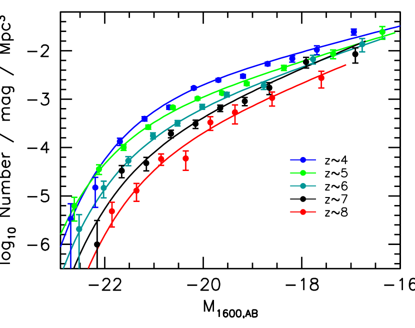
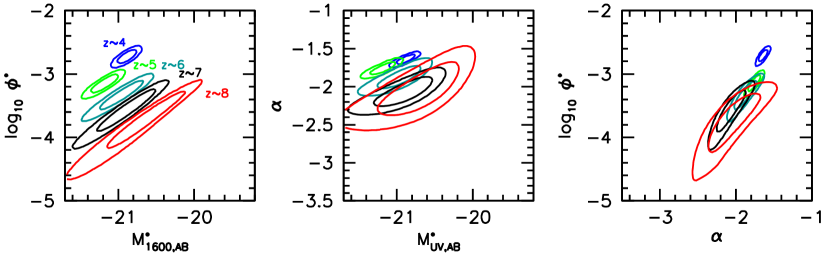
As in Bouwens et al. (2007) and Bouwens et al. (2011), we can write the stepwise LF as where is an index running over the magnitude bins, where corresponds to the absolute magnitude at the center of each bin, where
| (1) |
and where gives the position within a magnitude bin (for a 0.5-mag binning scheme). The goal then is to find the LF which maximizes the likelihood of reproducing the observed source counts over our various search fields. The likelihood can be expressed analytically as
| (2) |
where
| (3) |
where the above products runs over the different search fields and magnitude interval used in the LF determinations, is the expected number of sources in magnitude interval for a given LF, and is the observed number of sources in magnitude interval . The quantity is derived using the apparent magnitude of the source closest to 1600Å, which occurs in the band for sources in our samples, in the band for our and samples,131313Even though the -band magnitude of sources in our sample is nominally closer to 1600Å rest frame, we elected to use the band flux due to the greater overall depth of these data in many of our data sets (particularly the XDF) in the band for our samples, and in the band for our samples. For the ERS and CANDELS UDS/COSMOS/EGS wide-area samples where no coverage is available, we make use of the -band and magnitudes, respectively, instead for our and samples. We apply a small correction to the apparent magnitude of individual sources (typically 0.1 mag) so that it corresponds to an effective rest-frame wavelength 1600Å. The correction we apply is based on the biweight mean Bouwens et al. (2014a) derive for galaxies with a given absolute magnitude and redshift. The quantity is also corrected for contamination using the simulations we describe in §3.5.5.
Similar to our previous work, we compute the number of sources expected in a given magnitude interval assuming a model LF as
| (4) |
where is the effective volume over which one could expect to find a source of absolute magnitude in the observed magnitude interval . We estimate for a given search field using an extensive suite of Monte-Carlo simulations where we add sources with an absolute magnitude to the different search fields and then see if we select a source with apparent magnitude . The factors implicitly correct for flux-boosting type effects that are important near the detection limits of our samples, whereby faint sources scatter to brighter apparent fluxes and thus into our samples.
Computing the relevant ’s for all of our samples and search fields required our running an extensive suite of Monte-Carlo simulations. In these simulations, large numbers of artificial sources were inserted into the input data (typically 50 arcmin-2 in each simulation). Catalogs were then constructed from the data and sources selected. To ensure that the candidate galaxies in these simulations had realistic sizes and morphologies, we randomly selected similar-luminosity galaxies from the Hubble Ultra-Deep Field to use as a template to model the two-dimensional spatial profile for individual sources. We assigned each galaxy in our simulations a color using the vs. determinations of Bouwens et al. (2014a), with an intrinsic scatter in varying from 0.35 brightward of mag to 0.20 faintward of mag. This matches the intrinsic scatter in measured for brightest -5 sources by Bouwens et al. (2009, 2012) and Castellano et al. (2012), as well as the decreased scatter in for the faintest sources (Rogers et al. 2014). Finally, the templates were artificially redshifted to the redshift in the catalog using our well-tested “cloning” software (Bouwens et al. 1998; Bouwens et al. 2003a) and inserted these sources into the real observations. In projecting galaxies to higher redshift, we scaled source size approximately as to match that seen in the observations (Oesch et al. 2010a; Grazian et al. 2012; Ono et al. 2013; Holwerda et al. 2014b; Kawamata et al. 2014). We verified through a series of careful comparisons that the source sizes we utilized were similar to those in the real observations, both as a function of redshift and luminosity (Appendix D).
In calculating the effective selection volumes over the CANDELS-UDS, COSMOS, and EGS search areas, we also constructed fully simulated images of our mock sources in the ground-based and Spitzer/IRAC observations, adding these sources to the real observations, and extracting their fluxes using the same photometric procedure as we applied to the real observations. Finally, we made use of the full set of flux information we were able to derive for the mock sources (HST+ground-based+Spitzer/IRAC) to estimate photometric redshifts for these sources and hence determine whether sources fell within our redshift selection windows. As with the real observations, mock sources were excluded from the selection, if they were detected at 2.5 significance in passbands blueward of the break. We note that in producing simulated IRAC images for the mock sources, we assume a rest-frame EW of 300Å for H+[NII] emission and 500Å for [OIII]+H emission over the entire range -9, a flat rest-frame optical color, and a -optical continuum color of 0.2-0.3 mag, to match the observational results of Shim et al. (2011), Stark et al. (2013), González et al. (2012, 2014), Labbé et al. (2013), Smit et al. (2014a,b), and Oesch et al. (2013a).
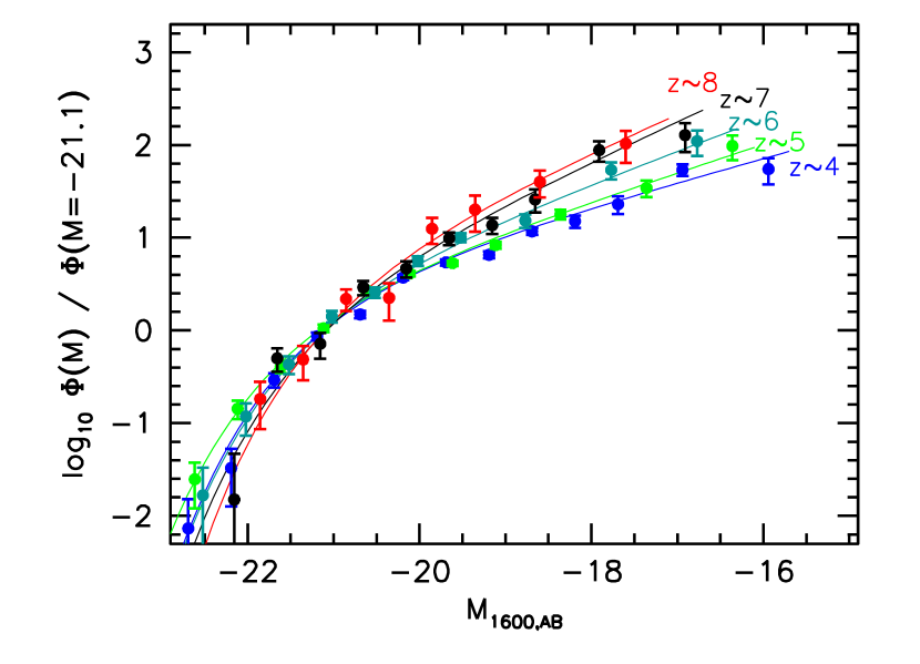
After deriving the shape of the LF at each redshift using this procedure, we set the normalization by requiring that the total number of sources predicted on the basis of our LF be equal to the total number of sources observed over our search fields. Applying the above SWML procedure to the observed surface densities of sources in our different search fields, we determined the maximum-likelihood LFs.
We elected to use a 0.5-mag binning scheme for the LFs at -8, consistent with past practice. To cope with the noise in our SWML LF determinations that result from deconvolving the transfer function (implicit in the term in Eq. 4) from the number counts , we have adopted a wider binning scheme at the faint-end of the LF. This issue also causes the uncertainties we derive on the bright end of the LF to remain somewhat large at all redshifts (as uncertainties in the measured flux for individual sources allow for the possibility that the observed source counts could arise from “picket fence”-type LF with the bulk of sources concentrated in just the odd or even stepwise LF intervals.)
In deriving the LF from such a diverse data set, it is essential to ensure that our LF determinations across this data set are generally self consistent. We therefore derived the LFs at , , , and separately from the wide-area UDS+COSMOS+EGS CANDELS observations, from the CANDELS-DEEP region within the CANDELS-GN and GS, from the CANDELS-WIDE region within the CANDELS-GN and GS, and from the BoRG/HIPPIES observations. As we demonstrate in Figure 23 from Appendix E, we find broad agreement between our LF determinations from all four data sets, suggesting that the impact of systematics on our LF results is quite limited in general.
After considering the LF results from each of our fields separately, we combine our search results from all fields under consideration to arrive at stepwise LFs at -8 for our overall sample. The results are presented in Figure 6 and in Table 5. Broadly speaking, the LF determinations over the range -8 show clear evidence for a steady build-up in the volume density and luminosity of galaxies with cosmic time.
4.2. Schechter Function-Fit Results
We next attempt to represent the LFs at , , , , , and using a Schechter-like parameterization ( ). Schechter functions exhibit a power-law-like slope at the faint end, with an exponential cut-off brightward of some characteristic magnitude . The Schechter parameterization has proven to be remarkably effective in fitting the luminosity function of galaxies at both low and high redshifts (e.g., Blanton et al. 2003; Reddy & Steidel 2009).
The procedure we use to determine the best-fit Schechter parameters is that of Sandage, Tammann, & Yahil (1979) and has long been the method of choice in the literature. Like the SWML procedure of Efstathiou et al. (1988), this approach determines the LF shape that would most likely reproduces the observed surface density of galaxies in our many search fields. The approach is therefore highly robust against large-scale structure variations across the survey fields. As with the SWML approach, one must normalize the LF derived using this method in some way, and for this we require that the total number of sources observed across our search fields match the expected numbers.
We can make use of essentially the same procedure to derive the maximum likelihood Schechter parameters as we used for the stepwise LF in the previous section, after we convert model Schechter parameters to the equivalent stepwise LF. For this calculation, we adopt a 0.1-mag binning scheme in comparing the stepwise LF to the surface density of sources in our search fields. A 0.1-mag binning scheme is sufficiently high resolution that it will yield essentially the same results as estimates made without binning the observations at all (e.g., Su et al. 2011).
Our maximum likelihood results for the Schechter fits at , , , , and are presented in Figure 7. Meanwhile, our best-fit Schechter parameters are presented in Table 6 using the XDF+HUDF09-Ps+ERS+CANDELS-GN+CANDELS-GS data set alone and using the full data set considered here. These Schechter parameters are also provided for the and LFs based on the full data set but excluding the CANDELS-EGS field, to indicate what the results would be excluding the large number of bright ( mag) galaxies found in that CANDELS field. Finally, in Table 9 from Appendix E, we also present determinations of the Schechter parameters from the CANDELS-GN+XDF+HUDF09-Ps fields and CANDELS-GS+ERS+XDF+HUDF09-Ps fields separately.
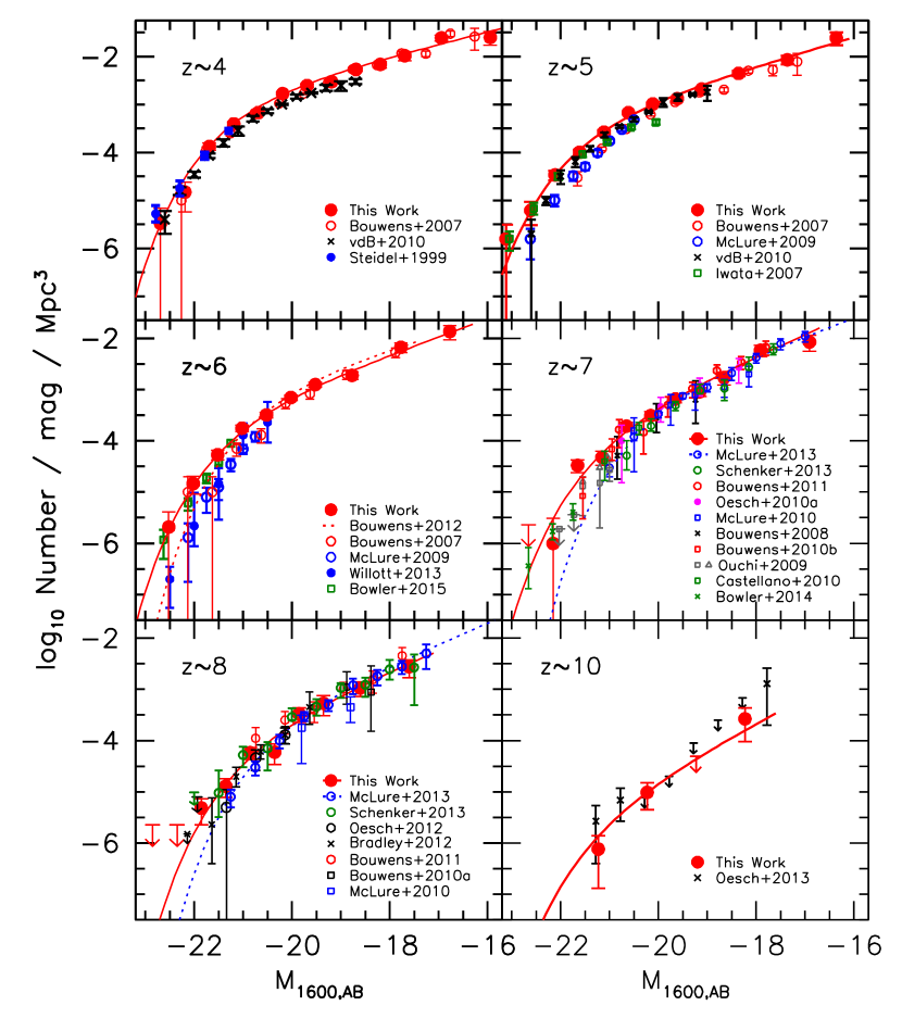
These results suggest that a good fraction of the evolution in the LF at may involve an evolution in both the normalization of the LF and the faint-end slope . Evolution in would be expected, if galaxies in arbitrarily massive halos in the early universe were capable of reaching the same maximum luminosity at essentially all epochs, independent of redshift. Evolution in the faint-end slope is also expected due to the steepening of the halo mass function towards early times (e.g., Trenti et al. 2010: see §5.5).
These general conclusions are not significantly impacted by possible systematic errors in our analysis technique. Even if we make factor-of-2 changes in the contamination rate across all of our search fields, we only find changes in the characteristic magnitude at -7 and changes in the normalization . While the impact on our faint-end slope estimates are larger, i.e., changes of 0.01, 0.03, 0.02, 0.10 at , , , and , respectively, these uncertainties are small relative to the overall evolution apparent from to . Larger changes in the characteristic magnitude are potentially possible (i.e., ), but for this to occur, contaminating sources must be systematically undercorrected so as to leave a excess in the number of bright galaxies. Small (10%) systematic errors in the selection volumes (per 0.5-mag interval) also likely have a small impact on the best-fit Schechter parameters.
Some earlier studies have argued that a simple evolutionary model may allow for a better representation of the evolution of the LF than an evolution in (Beckwith et al. 2006; van der Burg et al. 2010). At slightly higher redshifts (), McLure et al. (2010), Bouwens et al. (2011), McLure et al. (2013), and Oesch et al. (2014) all indicated that evolution may provide a slightly better description of the evolution of the LF. Of course, even distinguishing evolution in from over the range to can be challenging (as McLure et al. 2013 note explicitly).
While a pure evolutionary model seems quite effective at fitting the evolution at the bright end of the LF to high redshift, such a model does not capture the considerable steepening the LF experiences over a wide-luminosity baseline. Fitting this steepening requires either evolution in or evolution in as had been preferred by Bouwens et al. (2007). Yan & Windhorst (2004) effectively captured both aspects of the approximate evolution with their best-fit LF at (though they offer no clear justification in their analysis for their decision to fix to the value and to exclusively use the faint-end slope to model possible shape changes in the LF).
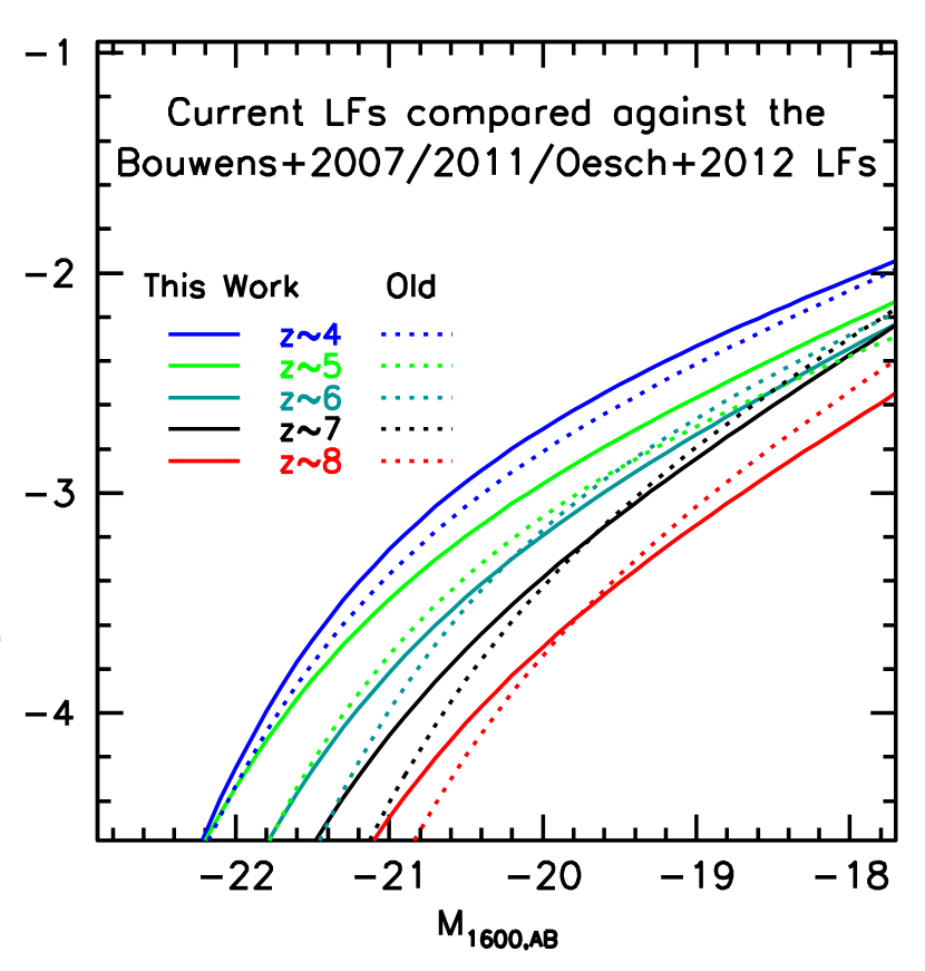
The present evolutionary scenario in and would appear to be quite different in form from the evolutionary scenario proposed by Bouwens et al. (2007), McLure et al. (2009), and Bouwens et al. (2011), which preferred evolution in the characteristic luminosity (particularly over the redshift range -6), with some evolution in and at (Bouwens et al. 2011; McLure et al. 2013). However, in detail, an + evolutionary scenario is not as different from evolution as one might think given their different parameterizations. Changes in the characteristic magnitude produce a similar steepening of the LF, as one can accomplish through changes in the faint-end slope .
Moreover, as we show in §5.3, the evolution in the luminosity we find for a galaxy (at a fixed cumulative number density) under the present + evolutionary scenario is essentially identical to what Bouwens et al. (2008) and Bouwens et al. (2011) found previously invoking an evolution in the characteristic magnitude (Figure 17). Unless one has very wide-area data to obtain tight constraints on the bright end of the LF at high redshift (such as one has with the wide-area CANDELS data set), one can trade off changes in the characteristic magnitude for changes in both and (without appreciably affecting the goodness of fit). We discuss these issues in more detail in Appendix F.2, F.3, F.6, and Figure 25.
An alternate way of looking at the evolution in the LF is by rescaling the volume densities of our derived LFs so that they have the same normalization at mag. We chose to rescale the LFs so they have the same normalization at this luminosity, which approximately corresponds to the value of at -7. This allows us to look for systematic changes in the shape of the LF without relying on a specific parameterization of the LF. The results are presented in Figure 8, and it is clear that the LF adopts an increasingly steep form at higher redshift. It is also clear that the volume density of galaxies at -7 does not fall off precipitously until brightward of mag.
4.3. Comparison against Previous Results
Before moving onto a discussion of possible non-Schechter-like features in the luminosity function, field-to-field variations, or our LF constraints at , it is useful to compare the present LF results with previous results from our own team (e.g., Bouwens et al. 2007; Bouwens et al. 2011; Oesch et al. 2012b; Oesch et al. 2014) as well as those from other groups. We include a comprehensive set of comparisons to previous results in Figure 9.
Overall, we find broad agreement with previous LF results over the full redshift range -10. However, there are also some noteworthy differences, particularly with regard to the volume densities of the most luminous -8 galaxies. In our current results, we find a higher volume density for luminous () -8 galaxies than reported earlier.
This significant update to our measurement of the volume density of high luminosity galaxies is the direct result of our lacking sufficiently deep () near-IR observations over very wide areas prior to the CANDELS program. With the new searches, we can now probe 15 more volume than was possible in our earlier -8 study (Bouwens et al. 2011) and 3 more volume than in our earlier Bouwens et al. (2007) -6 LF analysis. Our new LF results agree quite well with our earlier results, if we only consider the LF constraints over a range which were well constrainted by previous observations (Figure 10).
Differences with our previous constraints (Bouwens et al. 2007) can be attributed to the large increases in search volume, the availability of near-IR coverage to do a proper two-color selection of galaxies, and consistent coverage with HST to minimize the impact of systematics on our results, as one can verify by using the new WFC3/IR information to -correct previous results (Appendix F.2). The explanation for the observed differences with previous ground-based results (McLure et al. 2009; Willott et al. 2013) is less clear, but can at least partially be explained by uncertainties in deriving total luminosities from the -band fluxes (both from the IGM correction and -correcting the results to 1600Å: another 0.13-mag correction) and also possibly large field-to-field variance (Bowler et al. 2015). In any case, it is encouraging that our catalog and the Willott et al. (2013) catalogs agree quite well over the search fields where there is overlap (the brightest galaxies we find over the CANDELS COSMOS and EGS fields are exactly the same candidates as found by Willott et al. 2013 and we only miss one of the Willott et al. 2013 candidates over that field). It is also encouraging that new wide-area search results from Bowler et al. (2015) utilizing both the UltraVISTA and UDS fields are consistent with our determinations.
At , our LF results also indicate a much higher volume density of bright sources than indicated previously in Bouwens et al. (2011). However, this was largely due to our reliance on LF constraints available from the ground (e.g., from Ouchi et al. 2009; Castellano et al. 2010). If there was an overcorrection for contamination in those studies or the total magnitudes derived for sources were systematically fainter (0.1-0.2 mag) than those found here, it could explain the observed differences. We remark that our present constraints on and are in excellent agreement with the Bouwens et al. (2011b) constraints on those quantities if only the HST search results from that study are considered (Figure 8 from Bouwens et al. 2011 and Figure 26 from Appendix F.3).
Our new LF constraints also show a higher volume density of sources at mag than was previously found in either McLure et al. (2013), Schenker et al. (2013), or Bowler et al. (2014) studies. Differences with the McLure et al. (2013) and Schenker et al. (2013) results appear to occur due to -mag bias in the total magnitudes measured by McLure et al. (2013) and Schenker et al. (2013) for the brightest sources (see Figure 28 from Appendix H). Differences relative to Bowler et al. (2014) determinations over the UltraVISTA and UDS fields can potentially be explained, if Bowler et al. (2014) overestimated their completeness at the faint end of their probe, but we note that our constraint at mag is consistent with the Bowler et al. (2014) determinations. Moreover, it is encouraging that we identify exactly the same two galaxies over the CANDELS COSMOS area we probe as Bowler et al. (2014) find as part of their wide-area search ( candidates 268576 and 270128 from Bowler et al. 2014 lie over that region of the CANDELS COSMOS field that lacks deep optical ACS data and hence is not included in our search).
At , our new LF results are generally in excellent agreement with all previous HST studies. However, we do note a slight excess at the bright end of the LF relative to previous studies. This excess derives from three particularly bright ( mag) candidate galaxies found over the CANDELS EGS program. Each of these candidates appears very likely to be at , as they each have colors of 0.8 mag, very similar to that found by Ono et al. (2012), Finkelstein et al. (2013), and Laporte et al. (2014).
For a more extensive set of comparisons with previous work, we refer the reader to Appendix F.
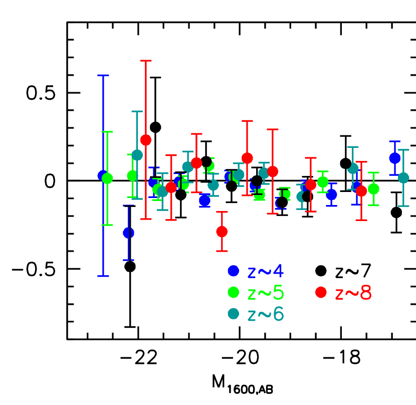
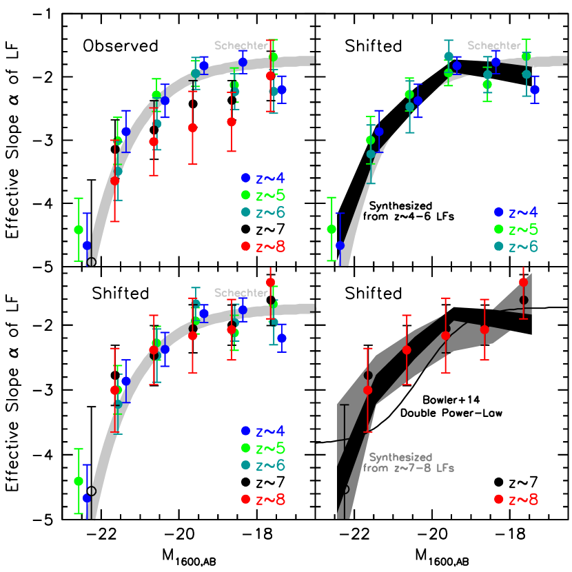
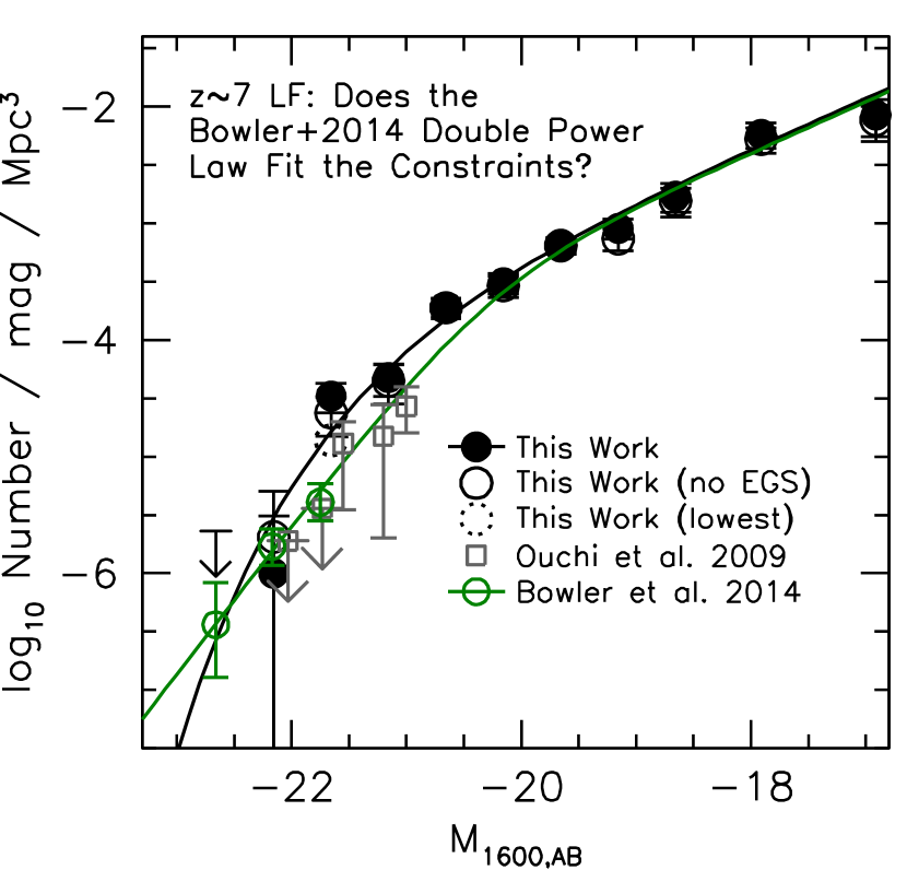
4.4. Non-Schechter-like Shape of the LF at ?
Several previous studies (Bowler et al. 2012; Bowler et al. 2014) have presented evidence that the LF at is not well represented by a Schechter function, but is rather better represented by a double power law:
Bowler et al. (2014) derive their constraints on the bright end of the LF from the UltraVISTA+UDS fields. If true, the Bowler et al. (2014) claim would be interesting, as it would imply that the LF at does not cut-off abruptly at a specific luminosity (as it would if the luminosity function were exponential), perhaps indicating that mass quenching or dust extinction were not as important early in the history of the universe as they were at later times.
The depth, area, and redshift range provided by our present samples put us in an unprecedented position to examine the general shape of the -8 LF and to see whether the LF is better represented by a Schechter-like function, a power law, a double power-law, or some other functional form.141414This is particularly true, given that we also partially make use of search constraints available from the deg2 LF analysis from Bowler et al. (2014). More precise constraints will eventually be possible, of course, integrating current HST constraints with even wider-area probes of the LF.151515Of course, to successfully make use of the very wide-area observations for such purposes, one must ensure that the total magnitude measurements and volume density measurements are made much more consistently than has generally been the case in the literature (with 0.1 mag systematic differences in the measured magnitudes being quite common: see Appendix F.2 and Skelton et al. 2014). Even 0.05 mag differences can result in 0.08 dex (20%) systematics in the LF assuming an effective slope of the LF of , which is typical at the bright end mag (see Figure 12).
There are at least two different facets to this endeavor. The first regards the shape of the LF at the bright end. Does the LF show an exponential-like cut-off at the bright end or is the bright end of the LF better represented by a steep power law? This was the question Bowler et al. (2014) attempted to answer. The second regards the shape of the LF at the faint end. Does the effective slope of the LF asymptote to a constant power-law slope (after modulation by an exponential), or does the effective slope of the LF show some dependence on luminosity even at very faint magnitudes? This second question was considered by Muñoz & Loeb (2011), as Figure 3 from their paper illustrates quite well.
Perhaps the easiest way to look for deviations from a Schechter-like form of the LF is by comparing the stepwise maximum-likelihood LF to the Schechter LF determined using the STY technique and computing the residuals as a function of luminosity. The result is shown in Figure 11. The lack of a significant trend relative to the best-fit Schechter functions suggest that the LFs at -8 can be described reasonably well with a Schechter function.
We can look at the overall functional form of the LF more directly by computing the effective slope of the LFs as a function of luminosity. This will allow us to assess whether other functional forms, i.e., a double power law, a rolling power law, or simple power law, also provide a reasonable representation of the LF. As with determinations of the LF itself, the effective slope of the LF can be derived over limited range in luminosity using the same maximum-likelihood technique as we used on the LF itself (i.e., by Sandage et al. 1979). For simplicity, we only attempt to derive these slopes at six distinct luminosities along the LF, i.e., , , , , , and .
In deriving the effective slope of the LF at these luminosities, we only consider sources 0.75 mag brighter and fainter than these luminosities, providing us with a total luminosity baseline for these slope measurements of 1.5 mag. Since this luminosity baseline is slightly longer than the separation between our slope measurements, we caution that the slope measurements we derive will not be entirely independent of each other. The longer luminosity baseline for each slope determination is quite useful, though, given the reductions in uncertainty on each slope measurement.
The result is shown in the panel of Figure 12 for the , , , , and LFs. Also shown on this figure (open black circle) is the effective slope of the LF at 22 mag by comparing our mag LF constraint with the volume density of mag galaxies obtained by Bowler et al. (2014). It is clear from these results that the effective slope of the LF at , , and is generally steeper than it is at -5. We already saw this in the fit results from the previous section.
To obtain a more precise constraint on the general shape of the LFs at -8, we can try to combine the constraints from the LFs at , , , , and considered individually. Motivated by the results from §4.2, perhaps the best way of accomplishing is to assume that the effective slope results at -8 LFs are all the same, modulo a change in the zero point (e.g., , , , ). If we do so and find the offsets that minimize the overall differences in the inverse-variance-weighted mean corrected offset at each redshift (specifically minimizing where indicates the effective slope measurements at a given absolute magnitude and redshift ), we find the following offsets in slope for the , , , and LFs relative to the LF: 0.01, 0.27, 0.37, and 0.64.
We then apply these offsets to the slopes of the , , , , and LFs shown in the top panel and show the result in the lower left panel of Figure 12. For context, we also show in Figure 12 the luminosity dependence we would expect adopting the typical Schechter function results derived in the previous section (shaded curve), with and . Overall, the constraints we have on the slope of the LF as a function of luminosity all appear to be remarkably similar to each other (after one removes the general offset in slope).
It is interesting to try to combine the constraints we have available on the -8 LFs to examine the overall form of the LF at . We examine the -6 case and the -8 cases separately, given possible evolution in both the shape and functional form of the LF. In the two cases, we compute the inverse-variance-weighted mean effective slope and variance as a function of luminosity (after removing the zero-point offset in effective slope).
The estimated 68% confidence intervals on the effective slope of the -6 and -8 LFs are indicated in the upper right and lower right panels of Figure 12 with the dark gray and light gray regions, respectively. In general, we find that our luminosity-dependent slope results are in broad agreement with the expectations of a Schechter function. At the low-luminosity end, we see no evidence for the effective slope of the LF being especially steeper at mag than at mag. This argues against the effective slope of the LF being strongly luminosity dependent, as one might expect if there is curvature in the halo mass function or if galaxy formation were less efficient at lower masses (e.g., Muñoz & Loeb 2011).
At high luminosities, the -6 LF show evidence for a similar exponential-like cut-off at bright magnitudes as that present in a Schechter function (compare the dark grey region in the upper left panel of Figure 12 with the light grey region). Not surprisingly, at -8, our overall constraints on the shape of the LF at high luminosities are much weaker and clearly not sufficient to constrain the functional form of the LF. However, our results do seem consistent with that observed at -6 and also adopting a Schechter function (compare the light grey region in the lower left panel with the dark grey region). For context, we also show the effective slope results implied from the Bowler et al. (2014) double power-law fit (shown in the lower right panel of Figure 12 as the solid black line), i.e., with , , , and Mpc-3 mag-1. While it is reasonable to imagine that the LF may exhibit a slightly non-Schechter shape at early enough times, we find no strong evidence for such a behavior here.
It is interesting to ask why our conclusions appear to differ from those of Bowler et al. (2014). For the purpose of this discussion, we compare our LF constraints with the double-power-law fit they find for their LF in Figure 13. While we find good agreement between the Bowler et al. (2014) power-law fit and our results at both the bright and faint ends, our LF is in excess of their double power-law fit at moderately high luminosities ( mag), suggesting this is the origin of our different conclusions.
How reliable are our LF constraints at mag? In the luminosity interval mag to mag, we find 16 galaxy candidates in total (3, 1, 1, 4, and 7 from the CANDELS-GS, GN, UDS, COSMOS, and EGS fields, respectively), so the uncertainties from shot noise (0.12 dex) are relatively limited. In addition, all 16 appear to be relatively robust -7.3 galaxy candidates, as inferred from the tests we run in Appendix G and §3.2.2-§3.2.3 (for distinguishing stars and galaxies). Nevertheless, there are other issues which could have an impact. If the large number of bright sources in the CANDELS-EGS field represent a rare overdensity and we exclude that field, if our total magnitude estimates are too bright by 0.1 mag, or if the completeness is underestimated (and it is instead 100%), then our -mag point in the LF would be lower by 0.15 dex, 0.09 dex, and 0.14 dex, respectively. Even if we assume all 3 issues to be the case (as a worst-case scenario), our LF estimates (open dotted circle in Figure 13) would only be lower by 0.38 dex and still be in tension with the Bowler et al. (2014) -mag point by 0.4 dex. Such a constraint, however, would be in excellent agreement with a Schechter fit to the LF at (but we note that fits to other functional forms would also be possible given the uncertainties).
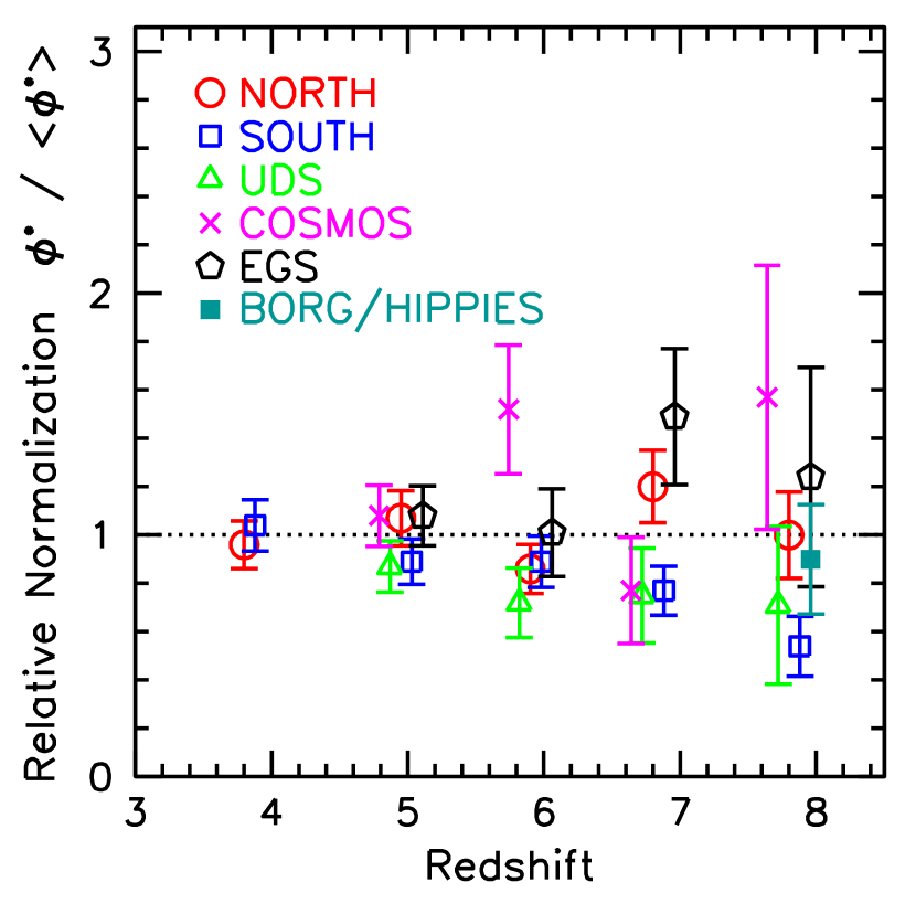
4.5. Field-to-Field Variations
One generic concern for the determination of any luminosity function is the presence of large-scale structure. As a result of such structure, the volume density of sources seen in one’s survey fields can lie significantly above or below that of the cosmic average – resulting in sizeable field-to-field variations. While normally these field-to-field variations introduce considerable uncertainties in our LF determinations, the availability of deep HST + ground-based observations over five independent survey fields allows us to largely overcome this issue. We estimate that the overall uncertainty on our LF results to be just 10%, by using the Trenti & Stiavelli (2008) cosmic variance calculator and accounting for the fact that we have observational constraints over 5 independent 150 arcmin2 search fields.
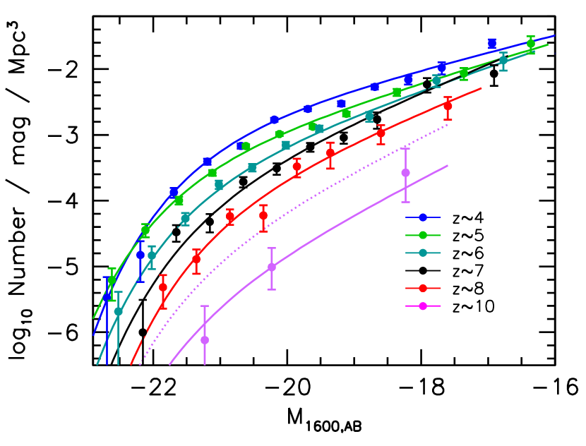
Due to the large number of independent search fields, we can perform a different test. Instead of our results on the LF being significantly limited by the impact of cosmic variance, we can use the current samples to set interesting constraints on the amplitude of the field-to-field variations themselves. For simplicity, we assume that we can capture all variations in the LF through a change in its normalization , keeping the characteristic magnitude and faint-end slope for galaxies at a given redshift fixed. The best-fit values for we derive for sources in each field relative to that found for all fields is shown in Figure 14 for sources in all five samples considered here. Bouwens et al. (2007) previously attempted to quantify the differences in surface densities of , , and sources over GOODS North and GOODS South (see also Bouwens et al. 2006 and Oesch et al. 2007). Uncertainties on the value of in a field relative to the average of all search fields is calculated based on the number of sources in each field assuming Poissonian uncertainties, allowing for small (10%) systematic errors in the calculated selection volumes field-to-field.
While the volume density of high-redshift candidates in most wide-area fields does not differ greatly (typically varying 20% field-to-field), there are still sizeable differences present for select samples field-to-field. One of the largest deviations from the cosmic average occurs for galaxies over the EGS field where the volume density appears to be almost double what it is over the CANDELS-GS, COSMOS, or UDS fields, for example. The CANDELS-GN also shows a similar excess at relative to these other fields (see also Finkelstein et al. 2013). The relative surface density of , , and candidates over the CANDELS-GN and GS fields are similar to what Bouwens et al. (2007) found previously (see Table B1 from that work), with the GS field showing a slight excess in and candidates relative to GN and the GN field showing an excess of candidates.
Generally however, the observed field-to-field variations are well within the expected 20% variations in volume densities for the large volumes probed in the present high-redshift samples.
4.6. LF Results
We also took advantage of our large search areas to set constraints on the LF at . Only a small number of candidates were found, but they still provide, along with the upper limits, a valuable addition to the -8. In doing so, we slightly update the recent LF results of Oesch et al. (2014) to consider the additional search area provided by the CANDELS-UDS, CANDELS-COSMOS, and CANDELS-EGS fields.
Due to the fact that the majority of our search fields contain zero candidates, we cannot use the bulk of the present fields to constrain the shape of the LF, making the SWML and STY fitting techniques less appropriate. In such cases, it can be useful to simply derive the LF assuming that the source counts are Poissonian-distributed (given that field-to-field variations will be smaller than the very large Poissonian uncertainties). One then maximizes the likelihood of both the stepwise and model LFs by comparing the observed surface density of candidates with the expected surface density of galaxies in the same way as we have done before (e.g., Bouwens et al. 2008).
Figure 15 shows the constraints we derive on the stepwise LF at based on the present searches (the results are also provided in Table 5). A 1-mag binning scheme is used, given the very small number of candidates in the present search. Also included on Figure 15 is our best-fit Schechter function at . For the latter fit, we fix the characteristic magnitude equal to and the faint-end slope to , consistent with the approximate characteristic magnitude and faint-end slope we estimate based on the LF fitting formula we present in §5.1.
The best-fit we estimate using our search over all of our search fields is Mpc-3. We tabulate this value of in Table 6. As we will discuss in Appendix F.5, the best-fit parameters we derive here are consistent with what Oesch et al. (2014) derived previously from a search over the CANDELS-GN+GS+XDF+HUDF09-Ps fields. These parameters are also consistent with the evolution in volume density that Oesch et al. (2013b, 2014) find from to .
5. Discussion
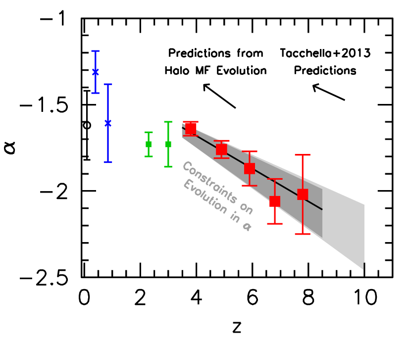
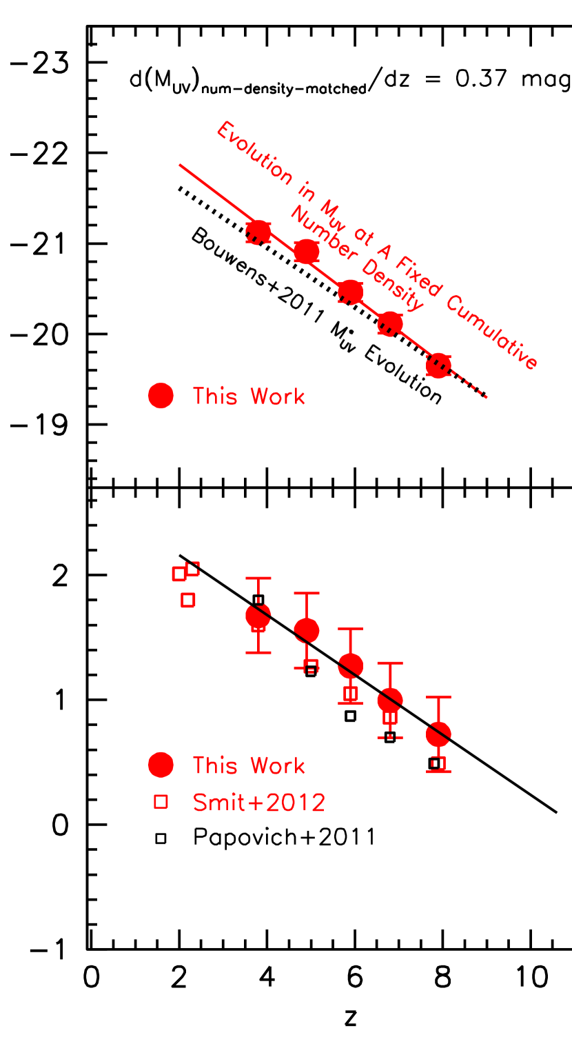
5.1. Empirical Fitting Formula for Interpolating and Extrapolating our LF Results to
As in previous work (e.g., Bouwens et al. 2008), it is useful to take the present constraints on the LF and condense them into a fitting formula for describing the evolution of the LF with cosmic time. This enterprise has utility not only for extrapolating the present results to , but also for interpolating between the present LF determinations at , , , , and when making use of a semi-empirical model. We will assume that each of the three Schechter parameter (, , ) depends linearly on redshift when deriving this formula. The resultant fitting formula is as follows:
Constraints from Reddy & Steidel (2009) on the faint-end slope of the LF at were included in deriving the above best-fit relations. As is evident from these relations, the evolution in the faint-end slope is significant at . The evolution in the normalization of the LF is significant at . We find no significant evolution in the value of .
Given the considerable degeneracies that exist between the Schechter parameters, it is also useful to derive the best-fit model if we fix the characteristic magnitude to some constant value and assume that all of the evolution in the effective shape of the LF is due to evolution in the faint-end slope . For these assumptions, the resultant fitting formula is as follows:
From this fitting formula, we can see that the steepening in the effective shape of the LF (as seen in Figure 8) appears to be significant at 5.7.
The apparent evolution in the faint-end slope is quite significant. Even if we allow for large factor-of-2 errors in the contamination rate or sizeable (%) uncertainties in the selection volume (as we consider in §4.2), the formal evolution is still significant at , while the apparent steepening of the LF presented in Figure 8 remains significant at (instead of ).
5.2. Faint-End Slope Evolution
The best-fit faint-end slopes we find in the present analysis are presented in Figure 16. The faint-end slope we determine is equal to , , and at , , and , respectively. Faint-end slopes of are very steep, and the integral flux from low luminosity sources can be very large since the luminosity density in this case is formally divergent. While clearly the LF must cut off at some luminosity, the light from galaxies fainter than 16 should dominate the overall luminosity density (Bouwens et al. 2012a).
In combination with the results at somewhat lower redshifts, the present results strongly argue for increasingly steep faint-end slopes at higher redshifts. Results from §5.1 suggest that this evolution is significant at if we consider just the formal evolution in the faint-end slope itself. The evolution is significant at if we consider the evolution in the shape of the LF (Figure 8).
| SFR density | ||||
|---|---|---|---|---|
| Dropout | (ergs s-1 | ( Mpc-3 yr-1) | ||
| Sample | Hz-1 Mpc-3) | Dust Uncorrected | Dust Corrected | |
| 3.8 | 26.520.06 | 0.06 | ||
| 4.9 | 26.300.06 | 0.06 | ||
| 5.9 | 26.100.06 | 0.06 | ||
| 6.8 | 25.980.06 | 0.06 | ||
| 7.9 | 25.670.06 | 0.07 | ||
| 10.4 | 24.62 | |||
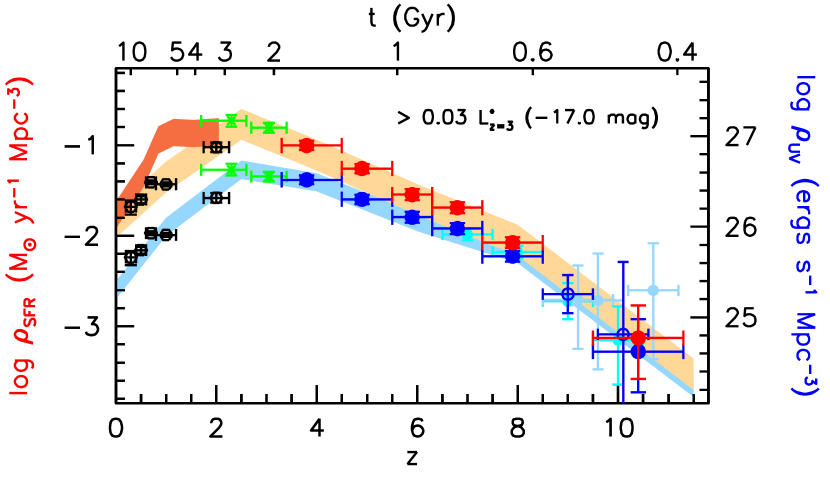
While consistent with previous results, the present results suggest slightly steeper faint-end slopes than reported in Bouwens et al. (2011), McLure et al. (2013), and Schenker et al. (2013) at . These steeper faint-end slope are a direct consequence of the somewhat brighter values for that we find in the current study and the trade-off between fainter values for and steeper faint-end slopes . These results only serve to strengthen earlier findings suggesting that the faint-end slope is steeper at (and likely ) than it is at . Similar conclusions have been drawn from follow-up work on gamma-ray hosts (Robertson et al. 2012; Trenti et al. 2012b; Tanvir et al. 2012; Trenti et al. 2013).
5.3. SFR Evolution in Individual Galaxies
Given the apparent evolution of the LF, one might ask how rapidly the luminosity or SFR of an individual galaxy likely increases with cosmic time. Fortunately, we can make progress on this question using a number density-matching procedure,161616Cumulative number-density matching can be a powerful way for following the evolution of individual galaxies with cosmic time. This is due to the fact that galaxies within a given volume of the universe largely grow in a self-similar fashion, so that th brightest or most massive galaxy at some point in cosmic time generally maintains its ranking in terms of brightness or mass at some later point in cosmic time (van Dokkum et al. 2010; Papovich et al. 2011; Lundgren et al. 2014). by ordering galaxies in terms of their observed luminosities and following the evolution of those sources with a fixed cumulative number density.
For convenience, we adopt the same integrated number density Mpc-3 (the approximate cumulative number density for galaxies) for this question as Papovich et al. (2011: see also Lundgren et al. 2014) had previously considered in quantifying the growth in the SFR of an individual galaxy with cosmic time. Dust corrections are performed using the measured ’s for galaxies at -8 (Bouwens et al. 2014a) and the well-known IRX- relationship from Meurer et al. (1999).
The results are presented in Figure 17. The luminosity at a fixed cumulative number density evolves as . Interestingly enough, the evolution in the luminosity we infer for galaxies at some fixed cumulative number density is almost identical to what Bouwens et al. (2011) had previously inferred for the evolution in the characteristic magnitude with redshift (i.e., : dotted black line).
Upon reflection, it is clear why this must be so. For pure luminosity evolution, one would expect both the characteristic magnitude of the LF and the luminosity of individual galaxies to evolve in exactly the same manner. Even though we now see that such a scenario does not work for the brightest, rarest galaxies, one can nevertheless roughly parameterize the evolution of fainter galaxies assuming pure luminosity evolution. For these galaxies, the Bouwens et al. (2008, 2011) fitting formula for evolution works remarkably well in describing their steadily-increasing luminosities. In this way, the modeling of the evolution of the LF using evolution by Bouwens et al. (2008, 2011) – a treatment built on by Stark et al. (2009) – effectively foreshadowed later work using a sophisticated cumulative number density-matching formalism to trace the star-formation history of individual systems at (Papovich et al. 2011; Lundgren et al. 2014).
The SFR for a galaxy in this number density-matched scenario evolves as . The evolution in the SFR is remarkably similar to the relations found by Papovich et al. (2011) and Smit et al. (2012). Not surprisingly, the best-fit trends for galaxies with -like volume densities (i.e., at Mpc-3) show little dependence on the parameterization of the Schechter function and whether one fits the evolution through a change in or a change in and .
5.4. Luminosity and Star Formation Rate Densities
We will take advantage of our new LF determinations at -10 to provide updated measurements of the luminosity density at -10. As in previous work (Bouwens et al. 2007, 2008, 2011; Oesch et al. 2012), we only derive the luminosity density to the limiting luminosity probed by the current study at , i.e., mag (0.03 ), to keep these determinations as empirical as possible. Since this is slightly fainter than what one can probe in searches for galaxies at , we make a slight correction to our and results. The best-fit faint-end slope we find at is assumed in this correction. The use of even steeper faint-end slopes (i.e., ) as implied by our LF fitting formula in §5.1 would yield similar results, only increasing the luminosity density by 0.015 dex.
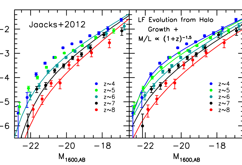
In combination with our estimates of the luminosity density, we also take this opportunity to provide updated measurements of the star formation rate density at -10. In making these estimates of the SFR density at -10, we correct for dust extinction using the well-known IRX- relationship (Meurer et al. 1999) combined with the latest measurements of from Bouwens et al. (2014a). As before, we assume that the extinction at rest-frame wavelengths is , with an intrinsic scatter of 0.35 in the distribution. This is consistent with what has been found for bright galaxies at -5 (Bouwens et al. 2012b; Castellano et al. 2012). The new determinations from Bouwens et al. (2014a) utilize large 4000-source samples constructed from the XDF, HUDF09-1, HUDF09-2, ERS, CANDELS-GN, and CANDELS-GS data sets and were constructed to provide much more accurate and robust measurements of the distribution than has been provided in the past. The mean dust extinction we estimate based on the Meurer et al. (1999) law for the observed distribution is 2.4, 2.2, 1.8, 1.66, 1.4, and 1.4 (in units of where and are the bolometric and UV luminosities of a galaxy, respectively) for the observed galaxies at , , , , , and , respectively.
The dust-corrected luminosity densities are then converted into SFR densities using the canonical Madau et al. (1998) and Kennicutt et al. (1998) relation:
| (5) |
where a - Salpeter IMF and a constant star formation rate for ages of Myr are assumed. In light of the very high EWs of the and [OIII] emission lines in -8 galaxies (Schaerer & de Barros 2009; Shim et al. 2011; Stark et al. 2013; Schenker et al. 2013; González et al. 2012; Labbé et al. 2013; Smit et al. 2014; González et al. 2014), it is probable that the adopted conversion factors underestimate the actual SFRs (perhaps by as much as a factor of 2: Castellano et al. 2014).
Our updated results on both the luminosity density and star-formation rate density are presented in Table 7 and Figure 18. As before, we have included select results from the literature (Schiminovich et al. 2005; Reddy & Steidel 2009) to show the trends at , as well as presenting recent determinations of the star formation rate density at -2.0 from IR bright sources (Daddi et al. 2009; Magnelli et al. 2009, 2011). We also include select results from the literature for comparison with previous results (Zheng et al. 2012; Coe et al. 2013; McLure et al. 2013; Ellis et al. 2013; Bouwens et al. 2014b).
We observe very good agreement with previous results over the full range in redshift -10. The most noteworthy changes occur at where the volume density we find is higher than estimated previously (Bouwens et al. 2007) and better matches the evolutionary trend connecting the and results. The improved robustness of the present results is likely a direct consequence of the significantly broader wavelength baseline available to select galaxies over the -5.5 volume than was available in the earlier purely optical/ACS data set (e.g., see discussion in Duncan et al. 2014).
5.5. Comparison with Theoretical Models
It is interesting to compare the current observational results with what is found from large hydrodynamical simulations and also from simple theoretical models. Such comparisons are useful for interpreting the present results and also for ascertaining whether any of our observational results are unexpected or challenge the current paradigm in any way. We first describe the models and then in the following subsections we discuss comparisons with our new LF results.
The first set of cosmological hydrodynamical simulations we consider are those from Jaacks et al. (2012). These results provide a very detailed investigation as to how the shape of the LF might evolve with cosmic time. Jaacks et al. (2012) make use of some large simulations done on a modified version of the GADGET-3 code (Springel et al. 2005) that includes cooling by H+He+metal line cooling, heating by a modified Haardt & Madau (1996) spectrum (Katz et al. 1996), an Eisenstein & Hu (1999) initial power spectrum, “Pressure model” star formation (Schaye & Dalla Vecchia 2008), supernovae feedback, and multiple-component variable velocity wind model (Choi & Nagamine 2011). Simulations are done with a range of box sizes from 10 Mpc to 100 Mpc ( or particles).
As an alternative to the results from large hydrodynamical simulations, we make use of a much more simple-minded theoretical model using a conditional luminosity function (CLF: Yang et al. 2003; Cooray & Milosavljević 2005) formalism where one derives the LF from the halo mass function using some mass-to-light kernel. We adopt the same CLF model as Bouwens et al. (2008) had previously used in their analysis of the LF, but have modified the model to include a faster evolution in the M/L of halos, i.e., . This evolution better reproduces changes in the observed LF from to . The factor also matches the expected evolution of the dynamical time scale. A detailed description of this model is provided in Appendix I. The advantage of this approach is that it can give us insight into the extent to which the evolution in the LF is driven by the growth of dark matter halos themselves and to what extent the evolution arises from changes in the mass-to-light ratio of those halos and hence gas dynamical processes (e.g., gas cooling or SFR time scales).
Finally, we consider the predictions by Tacchella et al. (2013), which are based on a minimal model that also links the evolution of the UV galaxy luminosity function to that of the dark-matter halo mass function. The model is constructed by assuming that a halo of mass at redshift has a stellar mass , of which a small fraction (10%) is formed at the halo assembly time , while the remaining is formed at a constant rate from to . Since halos have shorter assembly times as redshift increases, the UV light to halo mass ratio increases with redshift. describes the efficiency of the accretion in forming stars; Tacchella et al. (2013) calibrate it at via abundance matching.
Before conducting detailed comparisons of the observational results with the above theoretical models, we first present a comparison of the binned LF results with the first two theoretical models to illustrate the broad overall agreeement between the two sets of results (Figure 19).
5.5.1 Expected Evolution of the Faint-End Slope
The present observational results provide compelling evidence for significant evolution in the effective slope of the LF (Figure 8). While some of the evolution in the effective slope of the LF may be due to a change in the characteristic magnitude , most of the evolution appears to result from an evolving faint-end slope .
In comparing the present observational results with theory, let us assume that we can effectively parameterize the entire shape evolution of the LF using the faint-end slope (and because we do not finding convincing evidence for evolution in ). This assumption is useful, since it distills the shape information present in the moderately-degenerate + combination into a single parameter, resulting in a smaller formal error on the evolution. As shown in §5.1, we derive from the observations, if we force to be constant in our fits.
Remarkably enough, our simple-minded conditional LF model (Appendix I) is in remarkable agreement with our observational results, predicting that the faint-end slope of the LF evolves as . This compares with predicted from the Jaacks et al. (2012) simulation results. Finally, the Tacchella et al. (2013) model predict an evolutionary trend of . Each of these predictions is very similar to the observed evolution (see Figure 16) of .
5.5.2 Expected Evolution in the Characteristic Luminosity?
Our discovery of modest numbers of highly luminous galaxies in each of our high redshift samples, even at , provides strong evidence against a rapid evolution in the luminosity where the LF cuts off. Over the redshift range to , we find no significant evolution in (see Table 6). Over the slightly wider redshift range to , our best-fit estimate for the evolution in the characteristic magnitude is just (see the fitting formula in §5.1) or just from to . Given the observed luminosity of the brightest candidates found over the CANDELS fields (Oesch et al. 2014), i.e., mag, it seems unlikely that the bright-end cut-off is especially fainter than (limiting the evolution in to 1 mag over the redshift range -10).
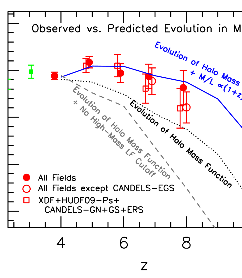
This implies that whatever physical mechanism imposes a cut-off at the bright end of LFs, this cut-off luminosity does not vary dramatically with redshift, at least out to . Indeed, for the three mechanisms discussed by Bouwens et al. (2008) to impose a cut-off at the bright end of the LF, i.e., heating from an AGN (Croton et al. 2005), the inefficiency of gas cooling for high-mass halos (e.g., Binney 1977; Rees & Ostriker 1977; Silk 1977), and the increasing importance of dust attenuation for the most luminous and likely most massive galaxies (Bouwens et al. 2009; Pannella et al. 2009; Reddy et al. 2010; Bouwens et al. 2012; Finkelstein et al. 2012; Bouwens et al. 2014a), there is no obvious reason any of these mechanisms should depend significantly on redshift or cosmic time.
Indeed, the results of the simulations or theoretical models bear out these expectations. The best-fit characteristic magnitudes derived from the Jaacks et al. (2012) simulations show very little evolution with cosmic time. Jaacks et al. (2012) derive , , and for their , , and LFs, respectively.
Simple fits to our CLF results also show only limited evolution in the characteristic magnitude with redshift, even out to . The characteristic magnitudes we derive from fitting the model LFs at -10 (minimizing the square of the logarithmic residuals) are presented in Figure 20 for comparison with our observational determinations of this same quantity (Table 6). Both a model assuming fixed mass-to-light ratios for the halos (black line) and a model with mass-to-light ratios evolving as the dynamical time (: blue line) are considered.
It is useful to contrast these results with a CLF model where no cut-off is imposed at the bright-end of the LF and where there is no evolution in the mass-to-light ratio of halos. For the model described in Appendix I, this could be achieved by replacing the term in Eq. I2 by unity and renormalizing the mass-to-light ratio so that for the model LF is equal to at . The evolution in the characteristic magnitude we would predict for this model is shown with the dashed gray line in Figure 20.
At sufficiently high redshift, it seems clear from the gray line that we would expect the characteristic magnitude to be fainter due to evolution in the halo mass function. In practice, however, the evolution in the characteristic magnitude may be more limited if the bright-end cut-off to the LF is instead set by a physical process that becomes dominant at some mass threshold (e.g., dust obscuration or quenching), as the dotted black line in Figure 20 illustrates. Even less evolution would be expected in the characteristic magnitude with cosmic time if halos at higher redshifts had systematically lower mass-to-light ratios, as illustrated by the blue line in this same figure.
In reality, of course, we should emphasize that almost all LFs predicted by simulations or CLF models can only be approximately modelled using a Schechter-function-like parameterization, and therefore there can be considerable ambiguity in actually extracting the Schechter parameters from the model results and hence representing their evolution with cosmic time.
6. Summary
The HUDF/XDF, HUDF09-1, HUDF09-2, ERS, and the five CANDELS fields contain a great wealth of deep, wide-area multiwavelength observations from the Hubble Space Telescopes and other facilities like Spitzer. Observations over these fields reach as deep as 30 mag (), cover a total area of 750 arcmin2, and include deep coverage in at least six passbands from HST and Spitzer, from 0.6-4.5m. 1000 arcmin2 area is leveraged in total including the BoRG/HIPPIES program. These exceptional depths, area, and quality make these fields a great resource for identifying galaxies over a wide range in both luminosity and redshift, from to .
Making use of this significant data set and a more efficient selection methodology we have developed, we have identified 10400 star-forming galaxies over the redshift range -10, including more than 698 probable galaxies at -8, and 6 candidate galaxies at . This is the largest such sample of galaxies assembled to date. The color criteria we introduce here for the selection of galaxies in the redshift range -10 now makes full use of the wavelength leverage available from the near-IR observations and has been optimized to be essentially complete, with no gaps in redshift between adjacent samples (Figure 1). This methodology produces comparably-sized samples and redshift segregation to what one can achieve segregating samples by their best-fit photometric redshifts, but retains the essential simplicity, reproducibility, and robustness against contamination that color criteria can particularly provide (§3.2).
We make use of these unprecedented samples to derive the LF in six distinct redshift intervals, at , , , , , and . We utilize essentially the same procedures as we previously utilized in Bouwens et al. (2007) and Bouwens et al. (2011). The selection volumes and selection efficiency for these samples are calculated by pixel-by-pixel redshifting actual galaxies from the HUDF to higher redshift according to the observed size-redshift relationship (Oesch et al. 2010; Ono et al. 2013), inserting these sources into the actual observations, and then attempting to reselect these sources and measure their properties using the same procedure that we use on the real observations. We explicitly verified that the size of the average sources in our simulations was well matched to the size of sources in the observations, as a function of both redshift and luminosity (Figure 22: Appendix D).
Five different types of contamination are considered for our samples, i.e., contamination from photometric scatter, contamination from stars, contamination from extreme emission line galaxies, contamination from supernovae, and contamination from spurious sources. We estimate a contamination level of 2%, 3%, 6%, 7%, and 10% for all but the faintest sources in our , , , , and samples, respectively. As in most of our previous studies, the only significant source of contamination is from the impact of noise on the photometry of individual sources (“photometric scatter”).
The low contamination rate is the result of great care being taken throughout the selection process to minimize the impact of potential contamination on our high-redshift samples. We validated our selection volume estimates in our wide-area fields, with a sophisticated set of degradation experiments, through the repeated addition of noise to our deepest data sets to match that found in our shallower data (§3.5.5). Similar use of these degradation experiments was made to determine the impact of higher noise levels on the total magnitudes measured for sources in our fields.
Extensive comparisons were made between the present LF results and some of the more noteworthy LF determinations from the literature (§4.3 and Appendix F). This is to provide us with the most comprehensive possible perspective from which to identify systematics in current and previous studies of the LF. In cases of differences, substantial effort was made to understand those differences, so as to make our final LF results as accurate as possible.
Our use of all five CANDELS fields to derive our high-redshift luminosity functions makes our results quite robust against the impact of cosmic variance, given that each CANDELS field provides us with an entirely independent sightline on the high redshift universe. The availability of different sightlines puts us in position to quantify the variation in the LF from field to field and therefore set accurate empirical constraints on the large-scale structure uncertainties (§4.5, Figure 14, and Appendix G).
Our conclusions are as follows:
-
•
Taking advantage of the widest-area systematic search for galaxies in the redshift range -10, we show that galaxies remain moderately prevalent (510-6 Mpc-3) to luminosities of mag over the entire redshift range to (§4.1). The volume density of galaxies only begins to fall off rapidly brightward of this magnitude. Sharp cut-offs in the LF were previously only found brightward of by van der Burg et al. (2010) for -5 samples and brightward of mag for samples by Willott et al. (2013) using the CFHT deep legacy survey fields.
-
•
While our -7 LFs are still in excellent agreement with our previous results over the range in luminosity and volume density well probed by our previous studies (Bouwens et al. 2007, 2008, 2011: Figure 10), the relatively robust constraints we have on the volume density of bright () galaxies at -8 from the wide-area CANDELS program allow for at most modest evolution in the characteristic magnitude with cosmic time (assuming a Schechter form for th LF). This suggests that whatever physical mechanism is responsible for imposing a cut-off in the LF at high luminosities (i.e., AGN feedback, inefficient gas cooling, high dust extinction) does not evolve dramatically with cosmic time (§5.5.2). The limited evolution in we observe is also consistent with the observational results of van der Burg et al. (2010) and simulation results of Jaacks et al. (2012).
-
•
We find significant evidence () for a steepening of the faint-end slope from at to at and at . Previously, some evidence for a steepening of the LF was presented by Bouwens et al. (2011), Su et al. (2011), Bradley et al. (2012), Schenker et al. (2013), McLure et al. (2013), and Calvi et al. (2013). The present study considerably strengthens the conclusions from these earlier studies, given the much tighter constraints we now have on the faint-end slope of the LF at -6 and self-consistent approach we have used to treat the LFs over the range to . The observed evolution appears to be in excellent agreement with that predicted from the steepening of the halo mass function (see §5.5.2), e.g., as seen in the results of Jaacks et al. (2012) and Tacchella et al. (2013).
-
•
Due to the strong limits we can set on the evolution in the characteristic magnitude from the current samples and the significant evolution in the LF itself with cosmic time, some evolution in the normalization of the LF appears to be required. From to , increases by nearly from 0.000008 Mpc-3 to 0.00197 Mpc-3 (see Figure 7 and Table 6: §4.2). While such a scenario might seem similar to that preferred by van der Burg et al. (2010) and Beckwith et al. (2006), a good fit to the overall evolution of the LF also requires considerable evolution in the steepness of the LF with cosmic time, as one can accomplish through a change in the faint-end slope (or also somewhat through changes in the characteristic magnitude ).
-
•
The best-fit characteristic magnitude we find for the LF at and is brighter than has been found in many previous studies (Bouwens et al. 2006; Bouwens et al. 2007; McLure et al. 2009; Su et al. 2011; Bouwens et al. 2011; Lorenzoni et al. 2011; Grazian et al. 2012; Willott et al. 2012; Schenker et al. 2013; McLure et al. 2013). The improved constraints at the bright end and larger numbers of sources show that the evolution in that has been widely accepted as the dominant change in the LF with time should be revised. Evolution in appears to be dominating the change in the LF with time. Interestingly, the evolution seen in , when combined with that found in , can be mimicked by an evolution in in noisier data, helping to clarify why the earlier, more limited datasets may have led to the the conclusion that was evolving (Appendix F.6).
-
•
Despite changes in the form of the evolution at the bright end of the LF, the best-fit evolution in preferred by Bouwens et al. (2008) and Bouwens et al. (2011) is in remarkably good agreement with the evolution in luminosity for the typical -bright galaxy (at a fixed cumulative number density: see §5.3 and Figure 17). The luminosity for such a number density-matched galaxy increases by 0.37 mag per unit redshift, which is almost identical to what Bouwens et al. (2008) and Bouwens et al. (2011) had inferred for the evolution in the characteristic magnitude of the LF over a similar redshift range to what we consider here. In this way, the schematic -evolutionary model of Bouwens et al. (2008) effectively foreshadowed later work using a cumulative number density-matched formalism to trace the steadily-increasing luminosities and star formation rates of individual galaxies (Papovich et al. 2011; Smit et al. 2012; Lundgren et al. 2014).
-
•
Our LF results appear to be perfectly consistent with the LF having a Schechter-like form over the entire redshift range -8 (§4.4). The consistency of our results with the Schechter form can be seen in Figure 11 where we present the differences between stepwise and Schechter representations of the LFs. We draw a similar conclusion looking at the effective slope of the -8 LFs, as a function of luminosity (Figure 12). We observe this both at high and low luminosities. At high luminosities, the LF exhibits a very similar exponential-like cut-off to that present in a Schechter function. At lower luminosities, the effective slope of the LF shows no significant change from to , consistent with this slope asymptoting to some fixed value. While our LF results are completely consistent with having a Schechter form (at both and -8), we cannot exclude the LF having an alternate functional form at (such as a double power-law shape: despite the clear tension between our LF results and those from Bowler et al. 2014). Although it is reasonable to imagine that the LF would exhibit a slightly non-Schechter shape at early enough times or at low enough luminosities (e.g., Muñoz & Loeb 2011), we find no strong evidence for such a behavior here.
-
•
The deep, wide-area search data over five independent sightlines in the high-redshift universe have made it possible for us to quantify the importance of field-to-field variations on the bright ends of the , , , , and LFs (§4.5). While most of our search fields show only modest differences (20%) in the volume density for sources at different redshifts, we find larger field-to-field variations in the volume density of galaxies in our samples at and , with the CANDELS-GN and EGS fields showing almost double the surface density of galaxies as the CANDELS-GS and UDS fields. The relative surface density of , , and galaxies we find over the CANDELS-GN and GS are in excellent agreement with the relative surface densities found previously by Bouwens et al. (2007).
-
•
We have taken advantage of our new LF constraints to derive a fitting formula to match the evolution seen in our sample over the redshift range to (§5.1). Our best fit relation is , , and . From this fitting formula, we find strong evidence for significant evolution in the volume density and . Evolution in the characteristic magnitude may be present, but it is less significant than found previously (Bouwens et al. 2008, 2011), as we noted above. Results from this fitting formula are in excellent agreement with our previous fitting formula (which preferred a more significant evolution) over the more limited range of luminosities and volume densities that was well probed by previous studies.
-
•
We find we can approximately match the evolution of the LF from to with a simple conditional luminosity function (CLF) model based on halo growth and a modest evolution in the mass-to-light ratio of the halos (§5.5). This CLF is successfully at reproducing the approximate evolution in all three Schechter parameters (see Figure 16, Figure 20, §5.5.1, and §5.5.2). The CLF model we present here is identical to the model we previously developed in Bouwens et al. (2008) except for the assumed evolution in the mass-to-light ratio of the halos.
The extraordinary depth, area, and wavelength baseline of the CANDELS, HUDF09, and HUDF12 data sets have provided us with substantial leverage to study the evolution of the LF with cosmic time. The most remarkable results of this study has been to demonstrate the progressive steepening of the LF to high redshift. As illustrated in Figure 8, the LF results at and are clearly much steeper than at and . Meanwhile, our use of 1000 arcmin2 search area along 5 independent sightlines (and numerous independent sightlines from the BoRG/HIPPIES pure parallel programs) has allowed us to demonstrate the existence of modest numbers of highly luminous ( mag) galaxies in the early universe at redshifts as high as (see also Oesch et al. 2014). The existence of such luminous galaxies at early times clearly demonstrates that the characteristic magnitude can only experience limited evolution with cosmic time.
In the future, we can expect stronger constraints on the evolution of the UV LF at -10 using data from the new Frontier Field Initiative, which will obtain 140 orbits of optical + near-IR observations over 4-6 cluster and parallel fields. These fields should be particularly effective in ensuring that current LF results are robust, since combining these new fields together with the 3 existing deep fields (XDF + two HUDF09-parallel) we will have 11-15 fields from which to map out the shape of the LF. The new Frontier Fields will also allow us to assess whether the results we have derived here based on the XDF and the HUDF09 parallel fields are representative and will add especially useful new constraints at -11.
References
- Adelberger & Steidel (2000) Adelberger, K. L., & Steidel, C. C. 2000, ApJ, 544, 218
- Alamo-Martínez et al. (2013) Alamo-Martínez, K. A., Blakeslee, J. P., Jee, M. J., et al. 2013, ApJ, 775, 20
- Anders & Fritze-v. Alvensleben (2003) Anders, P., & Fritze-v. Alvensleben, U. 2003, A&A, 401, 1063
- Arnouts et al. (2005) Arnouts, S., et al. 2005, ApJ, 619, L43
- Ashby et al. (2013) Ashby, M. L. N., Willner, S. P., Fazio, G. G., et al. 2013, ApJ, 769, 80
- Atek et al. (2011) Atek, H., Siana, B., Scarlata, C., et al. 2011, ApJ, 743, 121
- Beckwith et al. (2006) Beckwith, S. V. W., et al. 2006, AJ, 132, 1729
- Behroozi et al. (2013) Behroozi, P. S., Wechsler, R. H., & Conroy, C. 2013, ApJ, 770, 57
- Bertin and Arnouts (1996) Bertin, E. and Arnouts, S. 1996, A&AS, 117, 39
- Bielby et al. (2012) Bielby, R., Hudelot, P., McCracken, H. J., et al. 2012, A&A, 545, AA23
- Binney (1977) Binney, J. 1977, ApJ, 215, 483
- Birrer et al. (2014) Birrer, S., Lilly, S., Amara, A., Paranjape, A., & Refregier, A. 2014, ApJ, 793, 12
- Blakeslee et al. (2003) Blakeslee, J. P., Anderson, K. R., Meurer, G. R., Benítez, N., & Magee, D. 2003, Astronomical Data Analysis Software and Systems XII, 295, 257
- Blanton et al. (2003) Blanton, M. R., Hogg, D. W., Bahcall, N. A., et al. 2003, ApJ, 592, 819
- Bouwens, Broadhurst and Silk (1998) Bouwens, R., Broadhurst, T. and Silk, J. 1998, ApJ, 506, 557
- Bouwens et al. (2003) Bouwens, R., Broadhurst, T., & Illingworth, G. 2003a, ApJ, 593, 640
- Bouwens et al. (2003) Bouwens, R. J., Illingworth, G. D., Rosati, P., et al. 2003b, ApJ, 595, 589
- Bouwens et al. (2004) Bouwens, R. J., Illingworth, G. D., Thompson, R. I., et al. 2004a, ApJ, 606, L25
- Bouwens et al. (2004) Bouwens, R. J., Illingworth, G. D., Blakeslee, J. P., Broadhurst, T. J., & Franx, M. 2004b, ApJ, 611, L1
- Bouwens et al. (2006) Bouwens, R.J., Illingworth, G.D., Blakeslee, J.P., & Franx, M. 2006, ApJ, 653, 53
- Bouwens et al. (2007) Bouwens, R. J., Illingworth, G. D., Franx, M., & Ford, H. 2007, ApJ, 670, 928
- Bouwens et al. (2008) Bouwens, R. J., Illingworth, G. D., Franx, M., & Ford, H. 2008, ApJ, 686, 230
- Bouwens et al. (2009) Bouwens, R. J., et al. 2009, ApJ, 705, 936
- Bouwens et al. (2010) Bouwens, R. J., Illingworth, G. D., Oesch, P. A., et al. 2010a, ApJ, 709, L133
- Bouwens et al. (2010) Bouwens, R. J., et al. 2010b, ApJ, 725, 1587
- Bouwens et al. (2011) Bouwens, R. J., Illingworth, G. D., Labbe, I., et al. 2011a, Nature, 469, 504
- Bouwens et al. (2011) Bouwens, R. J., Illingworth, G. D., Oesch, P. A., et al. 2011b, ApJ, 737, 90
- Bouwens et al. (2012) Bouwens, R. J., Illingworth, G. D., Oesch, P. A., et al. 2012a, ApJ, 752, L5
- Bouwens et al. (2012) Bouwens, R. J., Illingworth, G. D., Oesch, P. A., et al. 2012b, ApJ, 754, 83
- Bouwens et al. (2013) Bouwens, R. J., Oesch, P. A., Illingworth, G. D., et al. 2013a, ApJ, 765, L16
- Bouwens et al. (2013) Bouwens, R. J., Illingworth, G. D., Oesch, P. A., et al. 2014a, ApJ, 793, 115
- Bouwens et al. (2012) Bouwens, R., Bradley, L., Zitrin, A., et al. 2014b, ApJ, 795, 126
- Bowler et al. (2012) Bowler, R. A. A., Dunlop, J. S., McLure, R. J., et al. 2012, MNRAS, 426, 2772
- Bowler et al. (2013) Bowler, R. A. A., Dunlop, J. S., McLure, R. J., et al. 2014, MNRAS, 440, 2810
- Bowler et al. (2014) Bowler, R. A. A., Dunlop, J. S., McLure, R. J., et al. 2015, MNRAS, arXiv:1411.2976, submitted
- Bradley et al. (2012) Bradley, L. D., Trenti, M., Oesch, P. A., et al. 2012, ApJ, 760, 108
- Bradley et al. (2014) Bradley, L. D., Zitrin, A., Coe, D., et al. 2014, ApJ, 792, 76
- Brammer et al. (2008) Brammer, G. B., van Dokkum, P. G., & Coppi, P. 2008, ApJ, 686, 1503
- Brammer et al. (2012) Brammer, G. B., van Dokkum, P. G., Franx, M., et al. 2012, ApJS, 200, 13
- Brammer et al. (2012) Brammer, G. B., Sánchez-Janssen, R., Labbé, I., et al. 2012a, ApJ, 758, L17
- Brammer et al. (2013) Brammer, G. B., van Dokkum, P. G., Illingworth, G. D., et al. 2013, ApJ, 765, L2
- Bruzual & Charlot (2003) Bruzual, G., & Charlot, S. 2003, MNRAS, 344, 1000
- Bunker et al. (2003) Bunker, A. J., Stanway, E. R., Ellis, R. S., McMahon, R. G., & McCarthy, P. J. 2003, MNRAS, 342, L47
- Bunker et al. (2004) Bunker, A. J., Stanway, E. R., Ellis, R. S., & McMahon, R. G. 2004, MNRAS, 355, 374
- Bunker et al. (2010) Bunker, A. J., Wilkins, S., Ellis, R. S., et al. 2010, MNRAS, 409, 855
- Burgasser et al. (2004) Burgasser, A. J., McElwain, M. W., Kirkpatrick, J. D., et al. 2004, AJ, 127, 2856
- Calvi et al. (2013) Calvi, V., Pizzella, A., Stiavelli, M., et al. 2013, MNRAS, 432, 3474
- Capak et al. (2004) Capak, P., Cowie, L. L., Hu, E. M., et al. 2004, AJ, 127, 180
- Capak et al. (2007) Capak, P., Aussel, H., Ajiki, M., et al. 2007, ApJS, 172, 99
- Capak (2008) Capak, P. L. 2008, Panoramic Views of Galaxy Formation and Evolution, 399, 54
- Capak et al. (2013) Capak, P., Faisst, A., Vieira, J. D., et al. 2013, ApJ, 773, L14
- Castellano et al. (2010) Castellano, M., et al. 2010, A&A, 524, A28
- Castellano et al. (2012) Castellano, M., Fontana, A., Grazian, A., et al. 2012, A&A, 540, A39
- Castellano et al. (2014) Castellano, M., Sommariva, V., Fontana, A., et al. 2014, A&A, 566, A19
- Chabrier (2003) Chabrier, G. 2003, PASP, 115, 763
- Choi & Nagamine (2011) Choi, J.-H., & Nagamine, K. 2011, MNRAS, 410, 2579
- Coe et al. (2013) Coe, D., Zitrin, A., Carrasco, M., et al. 2013, ApJ, 762, 32
- Coleman et al. (1980) Coleman, G. D., Wu, C.-C., & Weedman, D. W. 1980, ApJS, 43, 393
- Cooray & Milosavljević (2005) Cooray, A., & Milosavljević, M. 2005, ApJ, 627, L89
- Cooray & Ouchi (2006) Cooray, A., & Ouchi, M. 2006, MNRAS, 369, 1869
- Daddi et al. (2009) Daddi, E., et al. 2009, ApJ, 694, 1517
- Davis et al. (2007) Davis, M., Guhathakurta, P., Konidaris, N. P., et al. 2007, ApJ, 660, L1
- Dickinson (2000) Dickinson, M. 2000, Astronomy, physics and chemistry of H+3, 358, 2001
- Dickinson & GOODS Team (2004) Dickinson, M., & GOODS Team 2004, Bulletin of the American Astronomical Society, 36, #163.01
- Dickinson et al. (2004) Dickinson, M., Stern, D., Giavalisco, M., et al. 2004, ApJ, 600, L99
- Dijkstra et al. (2004) Dijkstra, M., Haiman, Z., Rees, M. J., & Weinberg, D. H. 2004, ApJ, 601, 666
- Dow-Hygelund et al. (2007) Dow-Hygelund, C. C., et al. 2007, ApJ, 660, 47
- Dressel et al. (2012) Dressel, L., et al. 2012. “Wide Field Camera 3 Instrument Handbook, Version 5.0” (Baltimore: STScI)
- Duncan et al. (2014) Duncan, K., Conselice, C. J., Mortlock, A., et al. 2014, MNRAS, 444, 2960
- Efstathiou et al. (1988) Efstathiou, G., Ellis, R. S., & Peterson, B. A. 1988, MNRAS, 232, 431
- Eisenstein & Hu (1999) Eisenstein, D. J., & Hu, W. 1999, ApJ, 511, 5
- Ellis et al. (2013) Ellis, R. S., McLure, R. J., Dunlop, J. S., et al. 2013, ApJ, 763, L7
- Ferguson et al. (2004) Ferguson, H. C. et al. 2004, ApJ, 600, L107
- Finkelstein et al. (2012) Finkelstein, S. L., Papovich, C., Salmon, B., et al. 2012, ApJ, 756, 164
- Finkelstein et al. (2013) Finkelstein, S. L., Papovich, C., Dickinson, M., et al. 2013, Nature, 502, 524
- Fontana et al. (2014) Fontana, A., Dunlop, J. S., Paris, D., et al. 2014, A&A, 570, AA11
- Ford et al. (2003) Ford, H. C., Clampin, M., Hartig, G. F., et al. 2003, Proc. SPIE, 4854, 81
- Furusawa et al. (2008) Furusawa, H., Kosugi, G., Akiyama, M., et al. 2008, ApJS, 176, 1
- Galametz et al. (2013) Galametz, A., Grazian, A., Fontana, A., et al. 2013, ApJS, 206, 10
- Giavalisco et al. (2004) Giavalisco, M., et al. 2004a, ApJ, 600, L93
- Giavalisco et al. (2004) Giavalisco, M., Dickinson, M., Ferguson, H. C., et al. 2004b, ApJ, 600, L103
- Giavalisco (2005) Giavalisco, M. 2005, New Astronomy Review, 49, 440
- González et al. (2012) González, V., Bouwens, R. J., Labbé, I., et al. 2012, ApJ, 755, 148
- González et al. (2014) González, V., Bouwens, R., Illingworth, G., et al. 2014, ApJ, 781, 34
- Grazian et al. (2011) Grazian, A., Castellano, M., Koekemoer, A. M., et al. 2011, A&A, 532, A33
- Grazian et al. (2012) Grazian, A., Castellano, M., Fontana, A., et al. 2012, A&A, 547, A51
- Grogin et al. (2011) Grogin, N. A., Kocevski, D. D., Faber, S. M., et al. 2011, ApJS, 197, 35
- Guo et al. (2013) Guo, Y., Ferguson, H. C., Giavalisco, M., et al. 2013, ApJS, 207, 24
- Haardt & Madau (1996) Haardt, F., & Madau, P. 1996, ApJ, 461, 20
- Holwerda et al. (2014) Holwerda, B. W., Trenti, M., Clarkson, W., et al. 2014a, ApJ, 788, 77
- Holwerda et al. (2014) Holwerda, B. W., Bouwens, R., Oesch, P., et al. 2014b, ApJ, submitted, arXiv:1406.1180
- Illingworth et al. (2013) Illingworth, G. D., Magee, D., Oesch, P. A., et al. 2013, ApJS, 209, 6
- Iwata et al. (2007) Iwata, I., Ohta, K., Tamura, N., et al. 2007, MNRAS, 376, 1557
- Jaacks et al. (2012) Jaacks, J., Choi, J.-H., Nagamine, K., Thompson, R., & Varghese, S. 2012, MNRAS, 420, 1606
- Kashikawa et al. (2004) Kashikawa, N., Shimasaku, K., Yasuda, N., et al. 2004, PASJ, 56, 1011
- Katz et al. (1996) Katz, N., Weinberg, D. H., Hernquist, L., & Miralda-Escude, J. 1996, ApJ, 457, L57
- Kawamata et al. (2014) Kawamata, R., Ishigaki, M., Shimasaku, K., Oguri, M., & Ouchi, M. 2014, ApJ, submitted, arXiv:1410.1535
- Kennicutt (1998) Kennicutt, R. C., Jr. 1998, ARA&A, 36, 189
- Kirkpatrick et al. (2011) Kirkpatrick, J. D., Cushing, M. C., Gelino, C. R., et al. 2011, ApJS, 197, 19
- Koekemoer et al. (2007) Koekemoer, A. M., Aussel, H., Calzetti, D., et al. 2007, ApJS, 172, 196
- Koekemoer et al. (2011) Koekemoer, A. M., Faber, S. M., Ferguson, H. C., et al. 2011, ApJS, 197, 36
- Koekemoer et al. (2013) Koekemoer, A. M., Ellis, R. S., McLure, R. J., et al. 2013, ApJS, 209, 3
- Kotulla et al. (2009) Kotulla, R., Fritze, U., Weilbacher, P., & Anders, P. 2009, MNRAS, 396, 462
- Kron (1980) Kron, R. G. 1980, ApJS, 43, 305
- Kuhlen & Faucher-Giguère (2012) Kuhlen, M., & Faucher-Giguère, C.-A. 2012, MNRAS, 423, 862
- Labbé et al. (2006) Labbé, I., Bouwens, R., Illingworth, G. D., & Franx, M. 2006, ApJ, 649, L67
- Labbé et al. (2010) Labbé, I., et al. 2010a, ApJ, 708, L26
- Labbé et al. (2010) Labbé, I., et al. 2010b, ApJ, 716, L103
- Labbé et al. (2013) Labbé, I., Oesch, P. A., Bouwens, R. J., et al. 2013, ApJ, 777, L19
- Laporte et al. (2014) Laporte, N., Streblyanska, A., Clement, B., et al. 2014, A&A, 562, L8
- Lawrence et al. (2007) Lawrence, A., Warren, S. J., Almaini, O., et al. 2007, MNRAS, 379, 1599
- Lehnert & Bremer (2003) Lehnert, M. D., & Bremer, M. 2003, ApJ, 593, 630
- Lorenzoni et al. (2011) Lorenzoni, S., Bunker, A. J., Wilkins, S. M., et al. 2011, MNRAS, 414, 1455
- Lorenzoni et al. (2013) Lorenzoni, S., Bunker, A. J., Wilkins, S. M., et al. 2013, MNRAS, 429, 150
- Lundgren et al. (2014) Lundgren, B. F., van Dokkum, P., Franx, M., et al. 2014, ApJ, 780, 34
- Madau et al. (1996) Madau, P., Ferguson, H. C., Dickinson, M. E., et al. 1996, MNRAS, 283, 1388
- Madau et al. (1998) Madau, P., Pozzetti, L. & Dickinson, M. 1998, ApJ, 498, 106
- Magee et al. (2011) Magee, D. K., Bouwens, R. J., & Illingworth, G. D. 2011, Astronomical Data Analysis Software and Systems XX, 442, 395
- Magnelli et al. (2009) Magnelli, B., Elbaz, D., Chary, R. R., Dickinson, M., Le Borgne, D., Frayer, D. T., & Willmer, C. N. A. 2009, A&A, 496, 57
- Magnelli et al. (2011) Magnelli, B., Elbaz, D., Chary, R. R., et al. 2011, A&A, 528, A35
- Martin et al. (2005) Martin, D. C., et al. 2005, ApJ, 619, L59
- McCracken et al. (2010) McCracken, H. J., Capak, P., Salvato, M., et al. 2010, ApJ, 708, 202
- McCracken et al. (2012) McCracken, H. J., Milvang-Jensen, B., Dunlop, J., et al. 2012, A&A, 544, A156
- McLure et al. (2009) McLure, R. J., Cirasuolo, M., Dunlop, J. S., Foucaud, S., & Almaini, O. 2009, MNRAS, 395, 2196
- McLure et al. (2010) McLure, R. J., Dunlop, J. S., Cirasuolo, M., et al. 2010, MNRAS, 403, 960
- McLure et al. (2013) McLure, R. J., Dunlop, J. S., Bowler, R. A. A., et al. 2013, MNRAS, 432, 2696
- Meurer et al. (1999) Meurer, G. R., Heckman, T. M., & Calzetti, D. 1999, ApJ, 521, 64
- Mosleh et al. (2012) Mosleh, M., Williams, R. J., Franx, M., et al. 2012, ApJ, 756, L12
- Moster et al. (2010) Moster, B. P., Somerville, R. S., Maulbetsch, C., et al. 2010, ApJ, 710, 903
- Muñoz & Loeb (2011) Muñoz, J. A., & Loeb, A. 2011, ApJ, 729, 99
- Nonino et al. (2009) Nonino, M., Dickinson, M., Rosati, P., et al. 2009, ApJS, 183, 244
- Oesch et al. (2007) Oesch, P. A., et al. 2007, ApJ, 671, 1212
- Oesch et al. (2009) Oesch, P. A., et al. 2009, ApJ, 690, 1350
- Oesch et al. (2010) Oesch, P.A., et al. 2010a, ApJ, 709, L16
- Oesch et al. (2010) Oesch, P. A., Bouwens, R. J., Carollo, C. M., et al. 2010b, ApJ, 709, L21
- Oesch et al. (2012) Oesch, P. A., Bouwens, R. J., Illingworth, G. D., et al. 2012a, ApJ, 745, 110
- Oesch et al. (2012) Oesch, P. A., Bouwens, R. J., Illingworth, G. D., et al. 2012b, ApJ, 759, 135
- Oesch et al. (2013) Oesch, P. A., Labbé, I., Bouwens, R. J., et al. 2013a, ApJ, 772, 136
- Oesch et al. (2013) Oesch, P. A., Bouwens, R. J., Illingworth, G. D., et al. 2013b, ApJ, 773, 75
- Oesch et al. (2014) Oesch, P. A., Bouwens, R. J., Illingworth, G. D., et al. 2014, ApJ, 786, 108
- Oke & Gunn (1983) Oke, J. B., & Gunn, J. E. 1983, ApJ, 266, 713
- Ono et al. (2012) Ono, Y., Ouchi, M., Mobasher, B., et al. 2012, ApJ, 744, 83
- Ono et al. (2013) Ono, Y., Ouchi, M., Curtis-Lake, E., et al. 2013, ApJ, 777, 155
- Ouchi et al. (2004) Ouchi, M., et al. 2004, ApJ, 611, 660
- Ouchi et al. (2009) Ouchi, M., Ono, Y., Egami, E., et al. 2009a, ApJ, 696, 1164
- Ouchi et al. (2009) Ouchi, M., et al. 2009b, ApJ, 706, 1136
- Pannella et al. (2009) Pannella, M., Carilli, C. L., Daddi, E., et al. 2009, ApJ, 698, L116
- Patten et al. (2006) Patten, B. M., Stauffer, J. R., Burrows, A., et al. 2006, ApJ, 651, 502
- Peng et al. (2002) Peng, C. Y., Ho, L. C., Impey, C. D., & Rix, H.-W. 2002, AJ, 124, 266
- Pirzkal et al. (2009) Pirzkal, N., Burgasser, A. J., Malhotra, S., et al. 2009, ApJ, 695, 1591
- Popesso et al. (2009) Popesso, P., et al. 2009, A&A, 494, 443
- Read et al. (2006) Read, J. I., Pontzen, A. P., & Viel, M. 2006, MNRAS, 371, 885
- Reddy et al. (2008) Reddy, N. A., Steidel, C. C., Pettini, M., et al. 2008, ApJS, 175, 48
- Reddy & Steidel (2009) Reddy, N. A., & Steidel, C. C. 2009, ApJ, 692, 778
- Reddy et al. (2010) Reddy, N. A., Erb, D. K., Pettini, M., Steidel, C. C., & Shapley, A. E. 2010, ApJ, 712, 1070
- Rees & Ostriker (1977) Rees, M. J., & Ostriker, J. P. 1977, MNRAS, 179, 541
- Riess et al. (2007) Riess, A. G., et al. 2007, ApJ, 659, 98
- Robertson & Ellis (2012) Robertson, B. E., & Ellis, R. S. 2012, ApJ, 744, 95
- Robertson et al. (2013) Robertson, B. E., Furlanetto, S. R., Schneider, E., et al. 2013, ApJ, 768, 71
- Rodney et al. (2014) Rodney, S. A., Riess, A. G., Strolger, L.-G., et al. 2014, AJ, 148, 13
- Rogers et al. (2014) Rogers, A. B., McLure, R. J., Dunlop, J. S., et al. 2014, MNRAS, 440, 3714
- Ryan et al. (2005) Ryan, R. E., Jr., Hathi, N. P., Cohen, S. H., & Windhorst, R. A. 2005, ApJ, 631, L159
- Sandage, Tammann, & Yahil (1979) Sandage, A., Tammann, G. A., & Yahil, A. 1979, ApJ, 232, 352
- Sawicki et al. (1997) Sawicki, M. J., Lin, H., & Yee, H. K. C. 1997, AJ, 113, 1
- Schlafly & Finkbeiner (2011) Schlafly, E. F., & Finkbeiner, D. P. 2011, ApJ, 737, 103
- Schaerer & de Barros (2009) Schaerer, D., & de Barros, S. 2009, A&A, 502, 423
- Schaye & Dalla Vecchia (2008) Schaye, J., & Dalla Vecchia, C. 2008, MNRAS, 383, 1210
- Schenker et al. (2013) Schenker, M. A., Robertson, B. E., Ellis, R. S., et al. 2013, ApJ, 768, 196
- Schiminovich et al. (2005) Schiminovich, D., et al. 2005, ApJ, 619, L47
- Schmidt et al. (2014) Schmidt, K. B., Treu, T., Trenti, M., et al. 2014, ApJ, 786, 57
- Scoville et al. (2007) Scoville, N., Abraham, R. G., Aussel, H., et al. 2007, ApJS, 172, 38
- Sheth & Tormen (1999) Sheth, R. K. & Tormen, G. 1999, MNRAS, 308, 119
- Shim et al. (2011) Shim, H., Chary, R.-R., Dickinson, M., et al. 2011, ApJ, 738, 69
- Shimizu et al. (2014) Shimizu, I., Inoue, A. K., Okamoto, T., & Yoshida, N. 2014, MNRAS, 440, 731
- Silk (1977) Silk, J. 1977, ApJ, 211, 638
- Skelton et al. (2014) Skelton, R. E., Whitaker, K. E., Momcheva, I. G., et al. 2014, ApJS, 214, 24
- Smit et al. (2012) Smit, R., Bouwens, R. J., Franx, M., et al. 2012, ApJ, 756, 14
- Smit et al. (2014) Smit, R., Bouwens, R. J., Labbé, I., et al. 2014a, ApJ, 784, 58
- Smit et al. (2014) Smit, R., Bouwens, R. J., Franx, M., et al. 2014b, ApJ, in press, arXiv:1412.0663
- Sobral et al. (2013) Sobral, D., Smail, I., Best, P. N., et al. 2013, MNRAS, 428, 1128
- Somerville et al. (2004) Somerville, R. S., Lee, K., Ferguson, H. C., et al. 2004, ApJ, 600, L171
- Springel (2005) Springel, V. 2005, MNRAS, 364, 1105
- Stanway, Bunker, & McMahon (2003) Stanway, E. R., Bunker, A. J., & McMahon, R. G. 2003, MNRAS, 342, 439
- Stanway et al. (2004) Stanway, E. R., Bunker, A. J., McMahon, R. G., et al. 2004, ApJ, 607, 704
- Stanway et al. (2005) Stanway, E. R., McMahon, R. G., & Bunker, A. J. 2005, MNRAS, 359, 1184
- Stark et al. (2009) Stark, D. P., Ellis, R. S., Bunker, A., Bundy, K., Targett, T., Benson, A., & Lacy, M. 2009, ApJ, 697, 1493
- Stark et al. (2010) Stark, D. P., Ellis, R. S., Chiu, K., Ouchi, M., & Bunker, A. 2010, MNRAS, 408, 1628
- Stark et al. (2013) Stark, D. P., Schenker, M. A., Ellis, R., et al. 2013, ApJ, 763, 129
- Steidel et al. (1996) Steidel, C. C., Giavalisco, M., Pettini, M., Dickinson, M., & Adelberger, K. L. 1996, ApJ, 462, L17
- Steidel et al. (1999) Steidel, C. C., Adelberger, K. L., Giavalisco, M., Dickinson, M. and Pettini, M. 1999, ApJ, 519, 1
- Steinhardt et al. (2014) Steinhardt, C. L., Speagle, J. S., Capak, P., et al. 2014, ApJ, 791, LL25
- Strolger et al. (2004) Strolger, L.-G., et al. 2004, ApJ, 613, 200
- Su et al. (2011) Su, J., Stiavelli, M., Oesch, P., et al. 2011, ApJ, 738, 123
- Szalay et al. (1999) Szalay, A. S., Connolly, A. J., & Szokoly, G. P. 1999, AJ, 117, 68
- Tacchella et al. (2013) Tacchella, S., Trenti, M., & Carollo, C. M. 2013, ApJ, 768, L37
- Tanvir et al. (2012) Tanvir, N. R., Levan, A. J., Fruchter, A. S., et al. 2012, ApJ, 754, 46
- Teplitz et al. (2013) Teplitz, H. I., Rafelski, M., Kurczynski, P., et al. 2013, AJ, 146, 159
- Tilvi et al. (2013) Tilvi, V., Papovich, C., Tran, K.-V. H., et al. 2013, ApJ, 768, 56
- Trenti & Stiavelli (2008) Trenti, M., & Stiavelli, M. 2008, ApJ, 676, 767
- Trenti et al. (2010) Trenti, M., Stiavelli, M., Bouwens, R. J., et al. 2010, ApJ, 714, L202
- Trenti et al. (2011) Trenti, M., Bradley, L. D., Stiavelli, M., et al. 2011, ApJ, 727, L39
- Trenti et al. (2012) Trenti, M., Bradley, L. D., Stiavelli, M., et al. 2012a, ApJ, 746, 55
- Trenti et al. (2012) Trenti, M., Perna, R., Levesque, E. M., Shull, J. M., & Stocke, J. T. 2012b, ApJ, 749, L38
- Trenti et al. (2013) Trenti, M., Perna, R., & Tacchella, S. 2013, ApJ, 773, L22
- Treyer et al. (1998) Treyer, M. A., Ellis, R. S., Milliard, B., Donas, J., & Bridges, T. J. 1998, MNRAS, 300, 303
- Vale & Ostriker (2004) Vale, A., & Ostriker, J. P. 2004, MNRAS, 353, 189
- van den Bosch et al. (2003) van den Bosch, F. C., Yang, X., & Mo, H. J. 2003, MNRAS, 340, 77
- van der Burg et al. (2010) van der Burg, R. F. J., Hildebrandt, H., & Erben, T. 2010, A&A, 523, A74
- van der Wel et al. (2011) van der Wel, A., Straughn, A. N., Rix, H.-W., et al. 2011, ApJ, 742, 111
- van Dokkum et al. (2010) van Dokkum, P. G., Whitaker, K. E., Brammer, G., et al. 2010, ApJ, 709, 1018
- Vanzella et al. (2009) Vanzella, E., et al. 2009, ApJ, 695, 1163
- Wang & Heckman (1996) Wang, B., & Heckman, T. M. 1996, ApJ, 457, 645
- Weiner & AGHAST Team (2014) Weiner, B. J., & AGHAST Team 2014, American Astronomical Society Meeting Abstracts #223, 223, #227.07
- Wilkins et al. (2010) Wilkins, S. M., Bunker, A. J., Ellis, R. S., et al. 2010, MNRAS, 403, 938
- Wilkins et al. (2011) Wilkins, S. M., Bunker, A. J., Stanway, E., Lorenzoni, S., & Caruana, J. 2011, MNRAS, 417, 717
- Willott et al. (2013) Willott, C. J., McLure, R. J., Hibon, P., et al. 2013, AJ, 145, 4
- Windhorst et al. (2011) Windhorst, R. A., Cohen, S. H., Hathi, N. P., et al. 2011, ApJS, 193, 27
- Yan & Windhorst (2004) Yan, H., & Windhorst, R. A. 2004, ApJ, 612, L93
- Yan et al. (2010) Yan, H.-J., Windhorst, R. A., Hathi, N. P., et al. 2010, Research in Astronomy and Astrophysics, 10, 867
- Yan et al. (2012) Yan, H., Finkelstein, S. L., Huang, K.-H., et al. 2012, ApJ, 761, 177
- Yang et al. (2003) Yang, X., Mo, H. J., & van den Bosch, F. C. 2003, MNRAS, 339, 1057
- Zheng et al. (2012) Zheng, W., Postman, M., Zitrin, A., et al. 2012, Nature, 489, 406 (Z12)
Appendix A A. Other Detailed Information on the Observational Data Sets that we utilize
A.1. A.1 Important Ground-Based Observations over the CANDELS UDS, COSMOS, and EGS Fields
The 450 arcmin2 region provided by the CANDELS UDS, EGS, and COSMOS fields provides valuable constraints on the volume density of the brightest, rarest sources at high redshift and as an additional control on the impact of field-to-field variations (“cosmic variance”) on the high-redshift luminosity functions.
To ensure that sources in our high-redshift selections were as free of lower redshift contamination as possible, we also made use of the very deep, optical ground-based data available over the three wide-area CANDELS fields. Deep observations at optical wavelengths are important for ensuring that high-redshift candidates exhibit a robust Lyman break and therefore are not likely at lower redshifts. For each of our fields, the ground-based imaging data reach as deep or deeper than the HST observations, particularly for extended sources (as most lower redshift contaminants typically are). Over both the CANDELS COSMOS and CANDELS EGS fields, we made use of the CFHT legacy survey deep observations in the , , , (“”), (“”), and bands.171717http://www.cfht.hawaii.edu/Science/CFHTLS Over the COSMOS field, we also made use of the very deep Subaru observations made available by Capak et al. (2007) in the , , , , , and bands. Finally, over the CANDELS UDS field, we made use of the very deep ( 28 mag depths at : -diameter apertures) Subaru observations taken as part of the Subaru XMM-Newton Deep Field (SXDF) program in the , , , , and bands (Furusawa et al. 2008).
Moderately deep -band and observations are available over the CANDELS-UDS and CANDELS-COSMOS fields with HAWK-I and VISTA, respectively, from the HUGS (Fontana et al. 2014) and UltraVISTA (McCracken et al. 2012) programs. The -band observations are of value for determining which -8 candidates from the CANDELS-UDS/COSMOS fields are more likely at and which are more likely at . The observations also provide us with useful information on the overall magnitude and spectral slope of candidates redward of the putative Lyman breaks. Our reduction of the HUGS observations is described in L. Spitler et al. (2014, in prep). Meanwhile, for a reduction of the three-year UltraVISTA observations, we use the official ESO release (http://www.eso.org/sci/observing/phase3/data_releases/uvista_dr2.pdf).
Intermediate-depth -band observations are available over the CANDELS EGS field from the WIRCam Deep Survey (McCracken et al. 2010; Bielby et al. 2012). While these observations only reach to 24.1 mag (1.2′′-diameter apertures) for the typical source over the CANDELS EGS field (Skelton et al. 2014), they do provide a probe of the spectral slope of galaxies redward of the CANDELS near-IR observations and therefore have some value in ascertaining the nature of the brightest sources over the CANDELS EGS field. We use these observations in deriving the best-fit redshifts for individual sources with EAZY.
A.2. A.2 BoRG/HIPPIES Fields
To obtain the most accurate constraints on the volume density of the rarest, brightest galaxies at , we also made use of the wide-area BoRG/HIPPIES pure-parallel programs (Trenti et al. 2011; Yan et al. 2011) and similar parallel data from the COS GTO team (Trenti et al. 2011). The BoRG/HIPPIES program features moderately deep observations (0.5 orbit to 3 orbit) in at least four different bands, i.e., /, /, , and bands, over a wide variety of different positions in the sky outside the galactic plane.
To ensure that the candidates we select from the BoRG/HIPPIES data set are robust, we only made use of the highest quality BoRG/HIPPIES fields, excluding those search fields with average exposure times in the bands of less than 1200 seconds or search fields where the exposure time in the optical or bands is less than the average exposure time in and observations.
The total search area in BoRG+HIPPIES and similar programs that satisfy both of these requirements was 218 arcmin2.
Where reductions are of the BoRG/HIPPIES search fields were already publicly available from Bradley et al. (2012: 0.08′′-pixel scale), we made use of those reductions. For the remaining search fields, the reductions were made using our wfc3red.py pipeline (Magee et al. 2011). We did not include the cycle-18 HIPPIES program (GO 12286: PI Yan) in our analysis due to the lack of the data and the challenge in selecting contamination-free galaxies over a similar redshift range as our other samples using the -band data from that program.
Though not formally part of the BoRG/HIPPIES program, we also incorporated the 28 orbits of parallel WFC3/IR observations over Abell 1689 (GO 11710: Alamo-Martínez et al. 2013) and the 18-orbit GO-12905 program (PI: Trenti) over the purported BoRG protocluster of galaxies (Trenti et al. 2012a; Schmidt et al. 2014) into the BoRG/HIPPIES data set, due to the similar filter choices available over these fields. The Abell 1689 parallel field has thus far not been used in searches for galaxies.
Appendix B B. Initial Photometric Set of -8 Candidates from the CANDELS-UDS, CANDELS-COSMOS, and CANDELS-EGS Fields
To derive our final of -8 candidates over the CANDELS UDS, COSMOS, and EGS fields, we first considered a selection of all those sources which satisfied Lyman-break-like selection criteria at , , and -8.
We selected these sources using the following color criteria
for our initial selection,
for our initial selection, and
for our initial -8 selection (similar to the color criteria adopted by Grazian et al. 2012). These color criteria were constructed in an analogous manner to the criteria we describe in §3.2.2 of this paper, such that sources entered the two color selection window at approximately the same redshift independent of the -continuum slope of the source. The color criteria for our initial , , and -8 selections are illustrated in Figure 21.
These criteria are used to identify the initial set of candidate -8 galaxies, to which we add deep ground-based optical+near-IR and Spitzer/IRAC photometry and measure photometric redshifts to derive our final , , , and samples (§3.2.3).

| Surface DensitybbThe surface densities of galaxies in a given magnitude interval are only estimated from fields that are largely complete in that magnitude interval. | Surface DensitybbThe surface densities of galaxies in a given magnitude interval are only estimated from fields that are largely complete in that magnitude interval. | Surface DensitybbThe surface densities of galaxies in a given magnitude interval are only estimated from fields that are largely complete in that magnitude interval. | |||
|---|---|---|---|---|---|
| Magnitude | (arcmin-2) | Magnitude | (arcmin-2) | Magnitude | (arcmin-2) |
| 0.0039aa upper limits | 0.0015aa upper limits | 0.0015aa upper limits | |||
| 0.0106 0.0061 | 0.0015aa upper limits | 0.0015aa upper limits | |||
| 0.0354 0.0112 | 0.0015aa upper limits | 0.0015aa upper limits | |||
| 0.2376 0.0290 | 0.0014 0.0014 | 0.0015aa upper limits | |||
| 0.6494 0.0480 | 0.0081 0.0033 | 0.0015aa upper limits | |||
| 1.4575 0.0718 | 0.0350 0.0069 | 0.0041 0.0023 | |||
| 2.4695 0.0935 | 0.0981 0.0115 | 0.0081 0.0033 | |||
| 3.7300 0.1627 | 0.2584 0.0419 | 0.0527 0.0190 | |||
| 4.7275 0.7609 | 0.3806 0.1638 | 0.1441 0.1019 | |||
| 6.6043 0.8993 | 1.0717 0.2749 | 0.4270 0.1754 | |||
| 6.5582 0.8962 | 1.2049 0.2915 | 0.4992 0.1897 | |||
| 8.3582 1.0117 | 1.8070 0.3570 | 0.6403 0.2148 | |||
| 10.4910 1.4912 | 2.9412 0.7896 | 1.0643 0.4908 | |||
| 16.8280 1.8886 | 5.8268 1.1113 | 1.3466 0.5520 | |||
| 10.7412 1.5089 | 4.5725 0.9845 | 1.6986 0.6200 | |||
| 2.0457 0.6585 | |||||
| 0.0015aa upper limits | 0.0014aa upper limits | ||||
| 0.0014 0.0014 | 0.0015aa upper limits | 0.0014aa upper limits | |||
| 0.0041 0.0023 | 0.0015aa upper limits | 0.0014aa upper limits | |||
| 0.0231 0.0055 | 0.0015aa upper limits | 0.0014aa upper limits | |||
| 0.0893 0.0110 | 0.0014 0.0014 | 0.0070 0.0070 | |||
| 0.2771 0.0194 | 0.0215 0.0054 | 0.0792aa upper limits | |||
| 0.5549 0.0274 | 0.0333 0.0067 | 0.2488aa upper limits | |||
| 1.1366 0.0884 | 0.1569 0.0327 | 0.4523 0.3198 | |||
| 1.9991 0.3950 | 0.2821 0.1411 | ||||
| 2.2056 0.4149 | 0.3527 0.1577 | ||||
| 3.1493 0.4958 | 0.8306 0.2420 | ||||
| 4.3133 0.5802 | 1.2726 0.2996 | ||||
| 4.6413 0.9919 | 1.2638 0.5176 | ||||
| 6.3116 1.1566 | 4.2857 0.9531 | ||||
| 5.2184 1.0517 | 3.4843 0.8594 | ||||
Appendix C C. Surface Density of -10 Galaxies
For convenience, we have calculated the surface density of -10 galaxy candidates found across all of our search fields and tabulated these surface densities in Table 8. In calculating the average surface density of sources over a given magnitude range, we have only included those regions from our multi-field probe where our simulations (§4.1) indicated we should be at least 80% complete relative to our completeness level at brighter magnitudes (i.e.,25 mag). This included our search results to 26 mag from all fields, results from our CANDELS-DEEP search fields to 27.0 mag, results from the HUDF09-1 and HUDF09-2 fields to 28.0 mag, and results from the XDF to 30.0 mag. While we would not expect the XDF results to be complete at 30 mag (it is expected to be similarly complete to 29), we quote the recovered surface density of sources in this field, since it represents our only probe of the surface density of galaxies to this magnitude level.
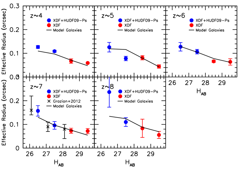
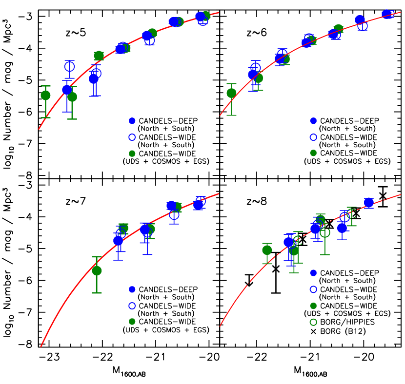
| XDF+HUDF09-Ps+CANDELS-GS+ERS | XDF+HUDF09-Ps+CANDELS-GN | ||||||
|---|---|---|---|---|---|---|---|
| Dropout | |||||||
| Sample | aaThe results in this table are derived in exactly the same way as the results in Table 5, but exclude the + search results over the CANDELS EGS field. While our simulation results (Figure 4) suggest that it is possible to identify and galaxies using the available observations over the CANDELS EGS field (albeit with some intercontamination between and samples), the lack of deep -band observations over this search field make the results less robust than over the other CANDELS fields. | Mpc-3) | aaThe results in this table are derived in exactly the same way as the results in Table 5, but exclude the + search results over the CANDELS EGS field. While our simulation results (Figure 4) suggest that it is possible to identify and galaxies using the available observations over the CANDELS EGS field (albeit with some intercontamination between and samples), the lack of deep -band observations over this search field make the results less robust than over the other CANDELS fields. | Mpc-3) | |||
| 3.8 | |||||||
| 4.9 | |||||||
| 5.9 | |||||||
| 6.8 | |||||||
| 7.9 | |||||||
Appendix D D. Ensuring the Model Size Distribution of Galaxies Matches the Observed Size Distribution
It is essential that we have an accurate measurement of the selection volume to obtain reliable estimates of the luminosity function at high redshift. The most important input for determining the selection volume for a high-redshift sample is the size or surface brightness distribution of the high-redshift star-forming galaxies from which the luminosity function is derived. Adopting sizes that are too large for model galaxies in the simulations will result in an underestimate of the selection volume, while adopting sizes that are too small for the model galaxies will result in an overestimate of the selection volume.
While this issue had already been considered in many studies of the LF (e.g., Bouwens et al. 2006; Oesch et al. 2007), Grazian et al. (2011) demonstrated the sizeable impact this issue could have determinations of the faint-end slope at -8, if not treated properly. Fortunately, care was taken in Bouwens et al. (2011), Schenker et al. (2013), and McLure et al. (2013) to ensure that the model galaxies in the simulations had a similar size distribution to what was used in the real observations (though the use of point-source profiles in deriving selection volumes by McLure et al. 2013 may result in a slight overestimate of the selection volume for bright galaxies).
To ensure an accurate match between the size distribution of galaxies in our simulations and that found in the observations, we subdivided galaxies in our -8 samples from the XDF+HUDF09-1+HUDF09-2 fields by their apparent -band magnitude and stacked the sources (after re-pixelating them to the same centroid position). We then measured their sizes using galfit (Peng et al. 2002). This process was then repeated using sources that we selected from the selection volume simulations described in §4.1. The two results are compared in Figure 22 as a function of the -band magnitude, for all of our high-redshift samples except our samples (where the small sample size precludes detailed comparisons). We experimented with the size scale of the HUDF galaxy we were using in the simulations until good agreement was obtained. The initial agreement was quite good, with the best match being obtained for sizes slightly (10%) smaller than expected from a scaling for fixed-luminosity sources.
| aaThe results in this table are derived in exactly the same way as the results in Table 5, but exclude the + search results over the CANDELS EGS field. While our simulation results (Figure 4) suggest that it is possible to identify and galaxies using the available observations over the CANDELS EGS field (albeit with some intercontamination between and samples), the lack of deep -band observations over this search field make the results less robust than over the other CANDELS fields. | (Mpc-3 mag-1) | bbDerived at a rest-frame wavelength of 1600Å. | (Mpc-3 mag-1) |
|---|---|---|---|
| galaxies | galaxies | ||
| 22.66 | 0.000003ccThe CANDELS-EGS field contains a much larger number of luminous () galaxy candidates than the other CANDELS fields (7 vs. 1, 2, 3, and 4) and may represent an extreme overdensity. Therefore, as an alternative to the present determination, we also provide a stepwise determination of the LF in Table 10 from Appendix E, which excludes the CANDELS-EGS data set. | 22.85 | 0.000003ccUpper limits are . |
| 22.16 | 0.0000020.000003 | 22.35 | 0.000003ccUpper limits are . |
| 21.66 | 0.0000240.000009 | 21.85 | 0.000003ccUpper limits are . |
| 21.16 | 0.0000450.000017 | 21.35 | 0.0000190.000007 |
| 20.66 | 0.0001890.000037 | 20.85 | 0.0000540.000016 |
| 20.16 | 0.0002930.000060 | 20.35 | 0.0000600.000026 |
| 19.66 | 0.0006450.000099 | 19.85 | 0.0003200.000100 |
| 19.16 | 0.0007400.000158 | 19.35 | 0.0004970.000212 |
| 18.66 | 0.0015660.000431 | 18.60 | 0.0010200.000340 |
| 17.91 | 0.0053000.001320 | 17.60 | 0.0026200.001000 |
| 16.91 | 0.0077200.002680 | ||
Appendix E E. Testing our -8 LF results for Internal Consistency
Given the large numbers of -8 galaxies that have been identified at , the entire enterprise of quantifying the LF at high redshift has increasingly become about minimizing the impact of systematic errors on one’s determination of the LF at high redshift.
To ensure that systematic errors in our high-redshift LFs are as small as possible, we have performed a considerable number of tests to ensure that our results are accurate and robust.
E.1. E.1 LF Results for Data Sets with Different Depths or Wavelength Coverage
One of the most important tests we performed was to divide our data set according to the depth, filter sets, and quality of data, to derive the LF on each data set independently, and then to compare the results to test for an overall consistency of the results.
We provide such a comparison in Figure 23 for our wide-area data sets, considering separately the 130 arcmin2 CANDELS-DEEP region over GOODS North and GOODS South, the 100 arcmin2 CANDELS-WIDE region over GOODS North and GOODS South, and the 450 arcmin2 CANDELS-WIDE region over the CANDELS-UDS, CANDELS-COSMOS, and CANDELS-EGS fields. Overall, our LF results show excellent consistency overall, particularly at the faint end and at , which is encouraging given significant differences in the depths and nature of the data sets used to derive the LFs.
However, at the bright end (), our stepwise determinations show larger differences. The most significant differences between our determinations appear to be at and . At , these differences appear to be partially the result of shot noise and large field-to-field variations in the volume densities of the brightest galaxies. In particular, we find 2 the surface density of bright () galaxies over the CANDELS-UDS, EGS, and COSMOS fields, as we find over the CANDELS-GN+GS+ERS fields. Slight differences in the -corrections we apply in deriving the absolute magnitude of galaxies at may contribute at a low level as well to the observed differences. For galaxies from the CANDELS-GS+GN+ERS fields, these magnitudes are derived based on the -band fluxes; however, for galaxies from the CANDELS-UDS+COSMOS+EGS fields, these magnitudes are derived from the -band fluxes.
At , we also observe noteworthy differences between our different determinations plotted in Figure 23. As was the situation at , these differences appear to arise from substantial differences in the surface density of bright galaxies, from field to field. The surface density of particularly bright galaxies is higher over the CANDELS-UDS/COSMOS/EGS fields as what it is over CANDELS-GN+GS+ERS fields.
In summary, our LF determinations generally show excellent consistency across the data sets considered in this analysis particularly at the faint end. While we do observe modest differences between our derived LFs at the bright end, these differences appear consistent with arising from large-scale structure variations.
E.2. E.2 Dependence of the LF Results on the GOODS Field Used for the Bright Constraints
A second test we performed was to compare the best-fit Schechter parameters for the LFs at , , , , and we derived for a variety of different search field combinations. The results are presented in Table 9. One of the comparisons we consider is to contrast the results from the XDF+HUDF09-Ps+CANDELS-GS+ERS data set with the XDF+HUDF09-Ps+CANDELS-GN data set. The best-fit Schechter parameters we derive from the two data sets are generally consistent with each other at .
However, the parameters do differ at 2 for the and LF determinations. The differences appear to be the result of the CANDELS-GN field showing a higher surface density of bright () galaxies as the CANDELS-GS+ERS field shows. Meanwhile, differences at appear to be explainable due to the higher surface densities of bright () galaxies in the CANDELS-GS+ERS field relative to the CANDELS-GN field.
E.3. E.3 LF Results for Our Entire Data Set Excluding the CANDELS-EGS field
Of all of our -8 samples over CANDELS, we find the most prominent excess of luminous galaxies at over the CANDELS-EGS field. It is possible that such an excess could act to skew our overall LF results and cause them to be less representative. A second concern is the lack of deep -band observations over the CANDELS-EGS field. While one can compensate for this by utilizing the Spitzer/IRAC [3.6][4.5] colors to distinguish galaxies from galaxies, this schema will not work for all galaxies (see Figure 4), and therefore we might expected some intercontamination between the bright samples over the CANDELS-EGS field and bright samples.
For these reasons, it is reasonable to quantify the LFs at and without including the CANDELS-EGS field. The stepwise results are provided in Table 10. Meanwhile, the best-fit Schechter LF results are placed in Table 6. While we find slight differences between these determinations and our primary determinations (Tables 10 and 6), the two results are fully consistent within the uncertainties. This is not surprising, as the two determinations are not independent.
Appendix F F. Comparisons against Previous -10 LF Determinations
Here we compare the present results with a few of the most noteworthy LF results at these redshifts from the literature in an attempt to understand the differences. For a comprehensive comparison with older LF results at -6 and -8, we refer the reader to Bouwens et al. (2007) and Bouwens et al. (2011).
Not only are the comparisons provided in this section useful for improving our confidence in the latest results, but they are also helpful for identifying biases that have existed in past work (most of which have occurred due to limitations in various data sets) to improve future determinations of the LF. Our new LFs differ from our previous LFs primarily because of the much larger number of bright objects from the wide-area CANDELS dataset which provide substantially more robust constraints at the bright end.
F.1. F.1 -5 Results
We compare the present LF determinations at -5 to select previous determinations in Figure 9. Included in the comparisons are the -5 LF results of Bouwens et al. (2007) using the GOODS+HUDF+HUDF-Parallel fields (Bouwens et al. 2004a), the LF results of Steidel et al. (1999) who make use of searches over 0.23 square degree, and the -5 LF results from van der Burg et al. (2010), who analyze the deep, wide-area (4 square degree) CFHT legacy survey deep field observations.
Our LF results at are in excellent agreement with the previous results from Bouwens et al. (2007) and also the results in Steidel et al. (1999) and van der Burg et al. (2010: though our best-fit Schechter function would appear to be 0.1 mag brightward of the van der Burg et al. 2010 stepwise constraints). Similar results were also obtained by Ouchi et al. (2004), Giavalisco (2005), and Yoshida et al. (2006) in the past, with the LFs of Ouchi et al. (2004) and Yoshida et al. (2006) only showing a modest excess in their faintest (and most uncertain) bin. Overall the results from these surveys are consistent in implying a value for around mag.
The present LF shows excellent agreement overall with the wide-area determination by van der Burg et al. (2010), except at mag where our LF determination is dex high (but consistent within the quoted errors), and with the determination by Iwata et al. (2007), except at the faint end of their search (where completeness and contamination are the most difficult to accurately model). At the faint end, our LF is generally 0.1 dex higher than the LF from Bouwens et al. (2007), but otherwise in reasonable agreement. The 0.1 dex difference likely resulted from Bouwens et al. (2007) underestimating the fraction of galaxies which would scatter outside their two color selection windows (see Duncan et al. 2014 for a discussion of the challenges) and hence overestimating the selection volume. The selection of galaxies using the full ACS+WFC3/IR photometry is much cleaner overall, making estimates of the selection volume more robust.
Our new LF is also in excess of the Bouwens et al. (2007) LF determination at the bright end. Such differences might again be attributed to Bouwens et al. (2007) overestimating their selection volumes. It is also possible that large-scale structure effects contributed (while here we efficiently probe the full redshift interval -5.5, most of Bouwens et al. 2007 selection volume derives from the redshift interval -5.0).
Our new LF results are also in excess of the McLure et al. (2009) determination at . We remark that differences with McLure et al. (2009) could be resolved if the magnitudes in the McLure et al. (2009) determination were systematically too faint (by 0.2 mag) or if the UDS field were substantially () underdense in bright galaxies. While such an underdensity over such a wide-area might seem implausible for standard models of large-scale structure or bias (e.g., Somerville et al. 2004; Trenti & Stiavelli 2008), Bowler et al. (2015) report evidence for 1.8 variations in the surface density of bright galaxies on square-degree scales, with the UDS being underdense relative to the UltraVISTA field. Interestingly enough, of all the CANDELS fields we consider, the CANDELS-UDS field appears to be among the poorest in bright ) galaxies, containing fewer bright galaxies than the CANDELS-COSMOS field.
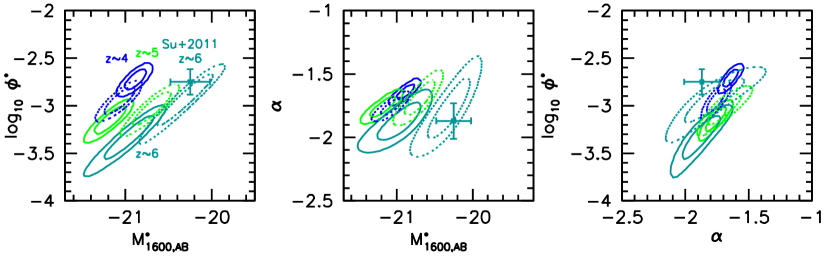
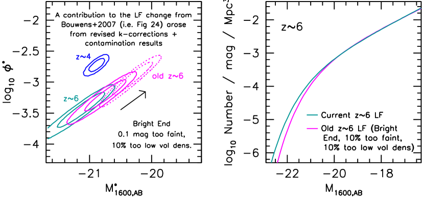
F.2. F.2 Results
The present LF results are in good agreement with the LF results of Bouwens et al. (2007) at the faint end (see Figure 9). At the bright end, however, the LF results of Bouwens et al. (2007) appear to be slightly lower than what we find here (albeit of only modest significance for most LF bins).
It is also useful to compare the present constraints on the Schechter parameters for the LF with the previous constraints on these parameters from Bouwens et al. (2007). Figure 24 presents both the 68% and 95% confidence intervals on these parameters, as derived by our two studies. Also included on this figure are the constraints that Su et al. (2011) using a similar ACS/optical data set, as Bouwens et al. (2011) utilize. There is a clear disagreement between the current constraints on the LF and previous constraints from Bouwens et al. (2007) and Su et al. (2011).
Given that we now have much better datasets at with deep near-IR coverage and also much larger bright samples, we can assess how the LFs at from the previous samples came to differ. This is an opportunity to assess and learn about what issues can arise with more limited datasets and does not indicate that the approach used then was inadequate, or that the current results are subject to significant systematic uncertainties.
After some investigation, we have concluded the differences largely arose due to Bouwens et al. (2007)’s only having ACS/optical data available to derive the rest-frame LF at (see also Su et al. 2011). This necessitated that (1) Bouwens et al. (2007) -correct the measured fluxes of their sources to 1600 to compare with LF results at -5, (2) Bouwens et al. (2007) correct their measured fluxes for IGM absorption (which is heavily dependent on the uncertain redshift distribution of candidates), and (3) Bouwens et al. (2007) correct for contamination of their selections made on the basis of the optical data alone. Each of these steps was uncertain and could have resulted in minor systematics in the derived Schechter parameters.
Indeed, one contributing factor appears to be the -correction that Bouwens et al. (2007) utilize in calculating the equivalent luminosity of sources at a rest-frame wavelength of 1600Å when the passband in which the sources were observed in the optical -band data had an equivalent rest-frame wavelength of 1350Å. Bouwens et al. (2007) derived the equivalent luminosity at 1600Å assuming a -continuum slope of based on the measurements available at that time (Stanway et al. 2005; Bouwens et al. 2006). However, as subsequent research has shown (Wilkins et al. 2011; Bouwens et al. 2012, 2014a; Finkelstein et al. 2012; Willott et al. 2013; Rogers et al. 2014), the most luminous galaxies have moderately red -continuum slopes . Use of the appropriate -continuum slopes by Bouwens et al. (2007) would have resulted in 0.1-mag higher estimates of the luminosity for bright sources than what Bouwens et al. (2007) used.
Another likely contributing factor is the correction that Bouwens et al. (2007) applied to account for contamination of their selection by -3 galaxies that were intrinsically red. Such corrections were necessary due to the lack of deep near-IR observations over the entire GOODS North and GOODS South areas, but could only be estimated from the deep ISAAC -band observations that were available over the GOODS South field. Bouwens et al. (2006) found that % of the sources brighter than 26 mag were likely contaminants using these near-IR observations and less than 2% faintward of 26 mag (see also Stanway et al. 2003 who estimated a 25% contamination rate for such a selection using sources from the GOODS South). Bouwens et al. (2007) made use of an almost identical correction. The availability of the deep WFC3/IR observations over the GOODS North and South allow us to directly test the accuracy of this correction. Using the new WFC3/IR imaging data to determine the nature of candidates in the Bouwens et al. (2007) catalogs, we find that 10.5% of the candidates brightward of mag have particularly red colors and appear likely to be lower redshifts contaminants.
To determine the effect of these systematics on the derived Schechter parameters at , we introduced similar systematics into the surface densities of candidates over CANDELS-GN and GS and rederived the Schechter parameters. The characteristic luminosity and we recovered is and Mpc-3 (0.4 mag fainter and higher than for our primary determinations). Interestingly, these Schechter parameters are consistent within with what we derived earlier in Bouwens et al. (2007: dotted magenta contours in Figure 25) for , i.e., , indicating it is possible to fully reconcile our present and previous results if we consider the above issues. See Figure 25 for details.
Bouwens et al. (2006) derived an even fainter characteristic luminosity and higher than Bouwens et al. (2007) derived, i.e., and Mpc-3. However, that determination of the Schechter parameters was biased by the procedure that Bouwens et al. (2006) used to correct for field-to-field variations. Small systematics in the degradation experiments resulted in the surface density of sources in the deeper fields being overcorrected upwards (by 10-15%) relative to the shallower fields. Even in the case of perfect corrections, Trenti & Stiavelli (2008) showed through extensive simulations that the procedure Bouwens et al. (2006) used to cope with large-scale structure result in minor biases in the measured , , and parameters (with too faint and too steep).
The present LF results at also imply a higher (2-3) volume density of luminous (-21.5 mag) galaxies than the recent results from McLure et al. (2009) and Willott et al. (2013). The McLure et al. (2009) probe utilizes the deep Subaru observations over the Subaru XMM-Newton Deep Field together the deep near-IR observations from the UKIDSS Ultra-Deep Survey, while the Willott et al. (2012) probe uses the full 4 square degree probed by the CFHT Legacy Survey deep fields. Given the very wide areas probed, it is unlikely that differences between our LF and previous determinations result from large-scale structure variations or shot noise (see Appendix G and Table 11).
At face value, this might suggest that previous ground-based probes of the LF were 90-99% incomplete (i.e., missing hundreds of bona-fide galaxies) or that the present probe contains large numbers of contaminants. However, explicit comparisons between the brightest candidates identified in the Willott et al. (2013) search over the CANDELS COSMOS and EGS regions and our own catalogs show very good agreement, as we describe in §3.4. Our catalog contains 3 of the 4 bright candidates identified by Willott et al. (2013) that fall within the CANDELS fields, i.e., WHM 14, WHM 15, and WHM 16. In addition, we find no sources which are brighter than the candidates common to both of our catalogs.
This suggests there must be some other explanation for the differences, as it is unlikely to arise from the composition of the bright samples (either from contamination or incompleteness in previous ground-based probes). One significant factor might be Willott et al. (2013) and McLure et al. (2009)’s use of deep -band observations to derive total luminosities for their sources, due to the impact of IGM absorption on the fluxes (significant in the -band at ) and -corrections required for comparisons with LFs derived at 1600Å. Both of these factors would tend to make the total luminosities of galaxies measured in Willott et al. (2013) and McLure et al. (2009) fainter than derived here, if not fully corrected. Use of the median colors of bright () -5.9 galaxies suggests a 0.13-mag correction from the -correction alone (i.e., from 1350Å to 1600Å). Absorption by the IGM would also lower the total luminosity inferred for individual sources (by 0.15 mag) if not fully corrected.
While one can speculate on the explanation for such differences in measurements of the total luminosity, clearly the new WFC3/IR data are much deeper than what was previously available and should allow for the best determinations of the total magnitudes. As a check on our total magnitude measurements, we have made a comparison with those from Skelton et al. (2014). For our brightest () candidate -8 galaxies over the CANDELS UDS/COSMOS/EGS fields, we find excellent overall agreement (with our magnitudes being just 0.04 mag brighter in the median).
Other possible explanations for differences include a slightly too aggressive removal of possible contaminating sources in previous studies (e.g., Figure 1 of Steinhardt et al. 2014 shows that photometric redshift techniques could err on the side of overcorrecting for contamination in -5 selections if not calibrated properly) or slight differences in the way total magnitudes were derived (with systematic differences catalog-to-catalog as large as 0.2 mag and more typically 0.1 mag: e.g., Figures 35-36 from Skelton et al. 2014). Of course, there is no reason to necessarily expect the total-magnitude measurements in ground-based probes to be too faint (as the blurring effect of the PSF makes flux measurements less sensitive to source size).
F.3. F.3 Results
The LF we derive at (Figure 9) is similar to previous determination of the LF at using the ERS and HUDF09 fields (Bouwens et al. 2011) given the uncertainties, but show a slightly larger volume density of bright sources. The larger volume density of bright galaxies is a direct result of the fact that the CANDELS-GN and EGS fields (Table 11) show a larger volume density of bright sources than were found within the 50 arcmin2 search area that we previously considered (from the ERS, HUDF/HUDF09, HUDF09-1, and HUDF09-2 search fields). The modest differences we observe at the bright end of the LF are not especially surprising as we are now probing 15 more volume at the bright end of the LF (and as many sightlines), as we did in the Bouwens et al. (2011) study.
The present LFs are in good agreement with the bright constraints set by the wide-area searches by Castellano et al. (2010) from HAWK-I (161 arcmin2: open green squares on Figure 9) and by Bouwens et al. (2010b) from NICMOS (88 arcmin2: open red squares on Figure 9). However, the present LF results show a -2 higher volume density for bright sources than was found by Ouchi et al. (2009b) in their wide-area (1568 arcmin2) search for galaxies over the Subaru Deep Field and GOODS North to 26 mag (grey open squares on Figure 9).
Given the seeming robustness of the present constraints on the bright end of the LF (due to the high quality of the present data set and large areas surveyed: see Appendix G), it would seem more likely that the issue lies with the Ouchi et al. (2009b) determination of the LF. One particular concern is the large (50%) contamination correction that Ouchi et al. (2009b) apply to their original sample of 22 sources in arriving at their final LF results. It is possible that the correction that Ouchi et al. (2009b) apply is too large. Even though Ouchi et al. (2009b) appear to have taken great care in accurately estimating the number of low-mass stars, lower-redshift interlopers, and spurious sources that would contaminate their probe, contamination correction are, by their very nature, highly uncertain, and Ouchi et al. (2009b) explicitly allow for the possibility that they have significantly overestimated the contamination rate by also presenting the LF without any contamination correction whatsoever (shown in Figure 9 as the grey open triangles). While this does not resolve the slight tension we observe with the brightest constraints from Ouchi et al. (2009b), where no contamination corrections were applied, such tensions could be resolved if there were slight differences (0.1-0.2 mag) between our measured magnitudes for the brightest sources and the magnitudes derived by Ouchi et al. (2009b: see Appendix F.2).181818In fact, Ono et al. (2012), themselves, concede that there is already some tension between the earlier LF results from Ouchi et al. (2009b) and the total magnitude [] they measure for a galaxy (GN-108036) found in the same search and for which they have spectroscopic confirmation.
The present LF also exhibits a higher volume density of bright sources than the recent LF determinations by Schenker et al. (2013) and McLure et al. (2013). There are two likely contributing factors that can account for this difference. One contributing factor is that the fact that the two wide-area fields used by these studies (CANDELS-GS and CANDELS-UDS fields) appear to be systematically underdense (by 1.5-2) in galaxies relative to two other search fields also included here, i.e., the CANDELS-EGS and CANDELS-GN fields (Figure 14). A second contributing factor is the HUDF12 team treating galaxy candidates as point sources in measuring their fluxes. The comparisons we present in Appendix H also suggest that the luminosities that Schenker et al. (2013) and McLure et al. (2013) derive for the brightest sources are 0.25 mag too faint in the median (see Figure 28). McLure et al. (2013)’s treating galaxies as point sources in deriving selection volumes for their LF could also contribute to differences between our two studies (perhaps 10% at the bright end). Together these issues could result in the HUDF12 team deriving a LF that shows a significantly fewer bright -7 sources.
Finally, the present LF results are in excellent agreement with the new LF determination at from Bowler et al. (2014), except for their faintest LF bin (see Figure 9). Bowler et al. (2014) derived their LF based on 34 candidates they identify over a 1.65 deg2 search area within the UltraVISTA and UKIDSS UDS search fields. It is unclear why the faintest LF bin from Bowler et al. (2014) is 0.8 dex lower than our own constraint at this luminosity. The three brightest candidates we find over the CANDELS regions of the COSMOS and UDS fields are exactly the same as Bowler et al. (2014) find, so differences in the derived LFs seem unlikely to arise from our finding especially bright sources that Bowler et al. (2014) miss. We do however find three fainter sources in the same magnitude interval that Bowler et al. (2014) do not find, suggesting that Bowler et al. (2014) may suffer from more incompleteness at the faint end than they estimate or the total magnitudes we measure for sources may be slightly brighter (0.1 mag) than what they recover. For the three sources our probes have in common, i.e., Bowler et al. (2014) candidates 211127 and 185070 and Himiko (Ouchi et al. 2009a), the total magnitudes we measure in the band are 0.10.3, 0.30.2 mags, and 0.10.1 mag brighter, respectively.
The best-fit value for the characteristic luminosity at () is brighter than what we presented in Bouwens et al. (2011: ). The lower value for presented by Bouwens et al. (2011: and similarly for Grazian et al. 2012) was largely driven by their use of the upper limits on the volume densities of bright sources from Ouchi et al. (2009b) based on their wide-area (1568 arcmin2) search for sources over the Subaru Deep Field and GOODS North. Excluding the wide-area constraints from Ouchi et al. (2009b) and the other wide-area searches (Castellano et al. 2010; Bouwens et al. 2010b), Bouwens et al. (2011) would have found a characteristic luminosity of (see Figure 26 and also Table 9).
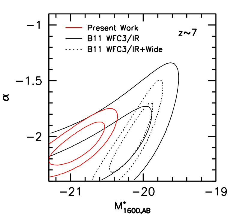
F.4. F.4 Results
The present results are in broad agreement with previous determinations of the LF at (Oesch et al. 2012; Yan et al. 2012; Bradley et al. 2012; Schenker et al. 2013; McLure et al. 2013; Schmidt et al. 2014), particularly at the faint end. However, we do find a slight excess at the bright end relative to other recent determinations, due to our discovery of three bright candidates over the CANDELS-EGS field. These bright candidates seem very likely to be at on the basis of their robustly red m-m colors.
In terms of the characteristic luminosity we derive, we find a much brighter value () than essentially all previous determinations: (Bouwens et al. 2011), (Oesch et al. 2012b), (Bradley et al. 2012), (McLure et al. 2013), (Schenker et al. 2013), (Schmidt et al. 2014), (Lorenzoni et al. 2011). However, we note that the value of we derive is consistent with what we would expect extrapolating from lower redshift, i.e., (§5.1). The bright value of we derive is a direct consequence of our discovery of three bright candidates identified over the CANDELS EGS field.
F.5. F.5 Results
While there are still considerable uncertainties in the determinations of the LF at , the present results are in excellent agreement with our earlier results as presented in Oesch et al. (2014), both in term of the binned points and the best-fit Schechter parameters (see Figure 9). This is particularly clear if we adopt the same shape for the LF as Oesch et al. (2014) use, i.e., and and if we restrict ourselves to the same samples and search fields. The best-fit value for that Oesch et al. (2014) find for these parameters is Mpc-3, while we find a best-fit value of Mpc-3.
F.6. F.6 How can we reconcile current findings with previous claims for a dominant evolution of the LF in at ?
Over the past few years, a wide variety of conclusions have been drawn regarding the evolution of the LF at high redshift. Some analyses have argued that the primary evolution in the LF is in (e.g., Bouwens et al. 2004a; Beckwith et al. 2006; Capak 2008), while other analyses have argued that the observations provide better support for a primary evolution in the characteristic luminosity (Bouwens et al. 2006; Bouwens et al. 2007; Bouwens et al. 2008; McLure et al. 2009; Lorenzoni et al. 2011) or the faint-end slope (Yan & Windhorst 2004).
One particularly influential analysis has been that of Bouwens et al. (2006) and Bouwens et al. (2007). In those analyses, it was found that the LF showed much stronger evolution at the bright end than it did at the faint end over the redshift interval to . The strong evolution Bouwens et al. (2006, 2007) found at the bright end was very similar to the evolution found earlier by Stanway et al. (2003) and Stanway et al. (2004), while the weaker evolution Bouwens et al. (2006, 2007) found at the faint end was in good agreement with the results of Giavalisco et al. (2004) and Bouwens et al. (2003b).
The luminosity-dependent evolution that Bouwens et al. (2006, 2007) observed could have been fit by an evolution in the faint-end slope of the LF or the characteristic luminosity . Of these two possibilities, Bouwens et al. (2006, 2007) found a better fit to the observed surface density of sources adopting an evolution in the characteristic luminosity. Subsequent analyses of both similar and even wider-area data sets (Su et al. 2011; McLure et al. 2009) recovered approximately the same set of Schechter parameters as what Bouwens et al. (2007) found.
The present LF determinations provide further evidence for such luminosity-dependent evolution. However, the large number of bright -7 galaxies and particularly galaxies found in the new wide-area WFC3/IR observations (Oesch et al. 2014) have made it clear that the general luminosity-dependent evolution can be better fit through an evolution in the faint-end slope and volume density , not exclusively with the characteristic magnitude as was originally found by Bouwens et al. (2006).191919Even though Beckwith et al. (2006) appear to have been generally correct in their use of to capture one aspect of the evolution of the LF, Beckwith et al. (2006) did not correctly capture the other aspect of the evolution of the LF, which is the very strong luminosity-dependent evolution (Figure 8). Beckwith et al. (2006) found no difference in the rate of evolution at the bright and faint ends of the LF.
Determining the exact form of the evolution of the LF at high redshift has been rather challenging for at least two reasons. First of all, the Schechter parameters become highly degenerate in cases of a steep faint-end slope , i.e., , due to the limited contrast between the faint-end slope of the LF and the effective slope of the LF at the bright end. This makes it more difficult to accurately measure the position of the knee of the LF (making the Schechter parameters highly degenerate). Second, accurate measurements of the position of the knee of the LF are further complicated by (1) field-to-field variations, (2) the large volumes one needs to probe to accurately determine the bright end of the LF, and (3) systematic errors. Systematic errors can affect determinations of the bright end of the LF differently than the faint end, due to the different data sets involved. Such errors can also have a different impact on determinations of the LF at -5 than at -8.
Of all of the above factors, perhaps the most challenging issue has been the substantial field-to-field variations in the surface densities of luminous sources. As Table 11 from Appendix G illustrates, the surface density of bright -8 galaxies appears to vary substantially depending upon where one happens to search. If one searches for bright -8 galaxies in fields which are underdense (as appears to have been the case over the CANDELS-GS), one would have inferred a faster evolution at the bright end of the LF (and hence ) than appears in fact to be present (using all five CANDELS fields). A comparison of the best-fit Schechter parameters based on the CANDELS-GN+GS (Table 6: upper rows) with the parameters derived from all of our search fields (Table 6: lower rows) suggests that this may have occurred.
Finally, if the LF at in fact has a non-Schechter shape, this could also have contributed to the past confusion regarding the overall evolution of the LF. Thus far, however, we find no evidence for such a non-Schechter form (§4.4).
The recent discovery of four bright (apparently robust) galaxies over the CANDELS-GN and GS by Oesch et al. (2014) leaves very little doubt as to how the LF at high redshift evolves. These bright galaxies simply cannot exist if the characteristic luminosity is the dominant variable explaining the evolution of the LF from to .
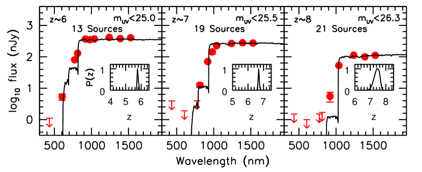
| Field | # | # | # | # |
|---|---|---|---|---|
| GOODS-S | 3 | 4 | 2 | 0 |
| GOODS-N | 1 | 2 | 5 | 1 |
| UDS | 0 | 2 | 3 | 0 |
| COSMOS | 3 | 4 | 4 | 0 |
| EGS | 4 | 7 | 5 | 0 |
| Total | 13ccThe other 2 bright candidates are found in the XDF and HUDF09-1 data sets. | 19 | 21ddWe required sources identified within the BoRG/HIPPIES data set to satisfy an even more stringent optical non-detection criteria () to effectively exclude all low-redshift interlopers from our selection.“*” indicates that for a flat redshift prior, the EAZY photometric redshift code (Brammer et al. 2008) estimates that this source shows at least a 68% probability for having a redshift significantly lower than the nominal low-redshift limit for a sample, i.e., , , , , , and for candidate , , , , , and galaxies, respectively. | 1 |
Appendix G G. Robustness of our Constraints on the Bright End of the -8 LFs
Particularly central to many conclusions in this paper regarding the shape of the LF at -8 concern the robustness of our constraints on the volume density of bright -8 galaxies. Such is an important question, given the tension between our results and several previous -7 results (though we note better agreement with the new Bowler et al. 2015 results).
To ensure that our results are well-determined, it is useful for us to look at the robustness of the redshift estimates we have on the brightest -8 sources and thus the contamination rate. We consider all candidates brighter than (13 sources), all candidates brighter than (19 sources), and all candidates brighter than (21 sources). We combined the flux measurements for all of the sources in these bright samples to produce a mean SED for each sample. The mean SED (presented in Figure 27) shows no evidence for flux blueward of the break (). Moreover, using the photometric redshift code EAZY to derive a redshift for the mean SED, we recovered , , and for the redshifts.
As a second check on the robustness of the redshifts for bright sources in our -8 samples, we used the photometric redshift code EAZY (Brammer et al. 2008) to compute their redshift likelihood distributions. Computing this distribution for all 57 individual sources in our bright samples and averaging the results, the average source showed just a 1.0% probability of corresponding to a galaxy. For the individual sources themselves, we found that all 53 bright candidates preferred a solution over a solution.
Second, we investigated how the measured volume density of the brightest -8 galaxy candidates varied from field to field. Since all five CANDELS fields have approximately the same selection volume for the brightest sources – given their similar areas and similar selectability of the brightest -8 candidates – the number of bright candidates per CANDELS field should provide us with an accurate estimate for the field-to-field variance in the volume density of bright -8 galaxies.
The total number of bright , , , and candidates in each of our search fields is given in Table 11. Interestingly enough, the number of bright candidates per field appears to show an approximate Poissonian distribution relative to the mean, with the most extreme upward deviation from the mean being the number of bright galaxies in the CANDELS-EGS field.202020Of course, we should emphasize that we would expect to find at least 7 bright galaxies in at least one of the 5 CANDELS fields 38% of the time – even assuming simple Poissonian statistics and the mean number of bright galaxies found across all 5 CANDELS fields.
Bootstrap resampling the number of bright candidates in each of the CANDELS fields, we find that the number of bright , , and candidates has a mean and uncertainty of 2.20.6 (0.12 dex), 3.81.0 (0.12 dex), and 3.80.6 (0.07 dex), respectively. Since the uncertainty here includes both the large-scale structure and Poissonian uncertainties, it provides our best estimate on the uncertainties in the volume density of the brightest -8 candidates.
In summary, all of our tests indicate that the volume density of bright -8 galaxies we derive is extremely robust.
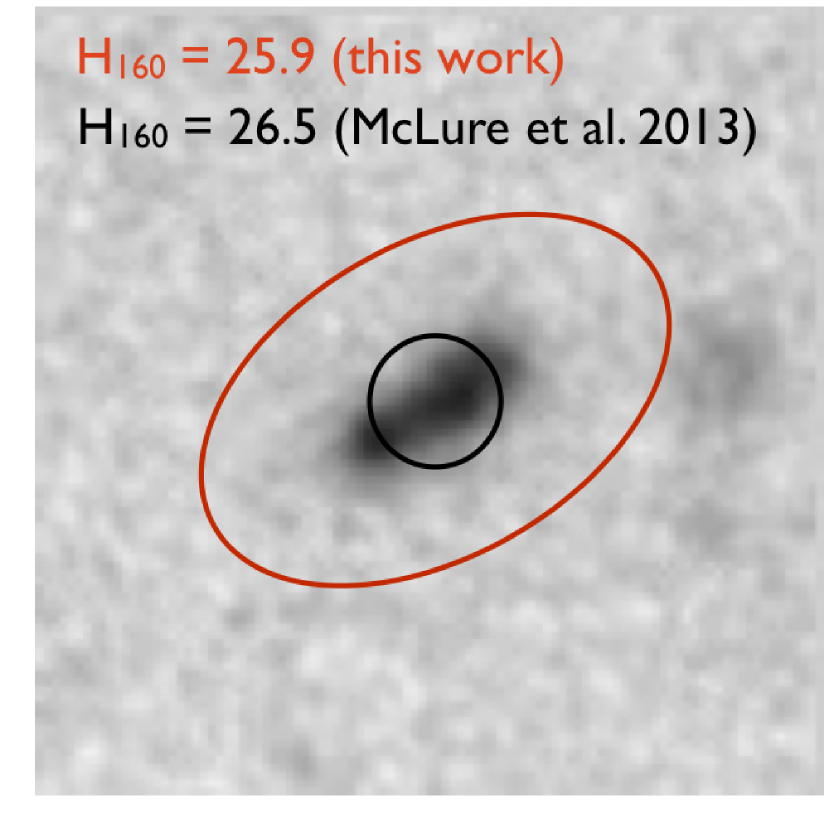
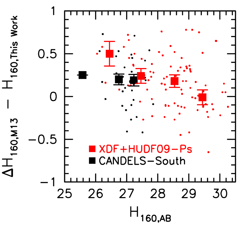
Appendix H H. Comparisons against the Total Magnitude Measurements from McLure et al. (2013)
One important difference between the methodology McLure et al. (2013) use to determine the LF at -8 and the procedure used here regard our procedures for measuring the total magnitudes of the sources. McLure et al. (2013) treat -8 galaxies as point sources, using fixed circular apertures enclosing 70% of the expected light for point sources and then applying a fixed 0.38-mag correction to total. We, however, derive total magnitudes for galaxies using the light inside 2.5 Kron radii (ranging from to in radius for 25 mag sources in CANDELS) and then applying an encircled energy correction appropriate for point sources.
To determine whether these differences in methodology may have resulted in any differences in measurements of the total magnitude, we matched up sources from the McLure et al. (2013) and the present catalogs and determined the difference in total -band magnitude. We present the differences in Figure 28 as a function of the average of the total magnitude measurements. Differences in the total magnitude measurements for sources from the deepest data sets XDF, HUDF09-1, HUDF09-2 are shown in separate colors from differences that occur for sources found in the CANDELS-GS and ERS data set, due to the slight dependence total magnitudes can show on the depth of a data set (when using variable apertures).
As is apparent from Figure 28, the total magnitude measurements from McLure et al. (2013) appear to agree quite well with our measurements for the faintest, lowest-luminosity -8 galaxies. However, for more luminous sources, the total magnitude measurements from McLure et al. (2013) are offset (in the median) by 0.25 mag faintward of our total magnitude measurements. While it might be surprising to see such large differences, biases would clearly be expected in the McLure et al. (2013) photometry for the largest, most extended sources (e.g., see the galaxy shown in the left panel of Figure 28). We verified that we could reproduce the quoted magnitudes in McLure et al. (2013) using similar -diameter aperture photometry and then aperture correcting the results.
We expect similar systematic biases in the Schenker et al. (2013) LF results due to their use of an identical photometric procedure.
Appendix I I. Bouwens et al. (2008) Conditional Luminosity Function Model
As an alternative to comparisons with the results from large hydrodynamical simulations (e.g., Jaacks et al. 2012), we make use of a much more simple-minded theoretical model using a conditional luminosity function (CLF: Yang et al. 2003; Cooray & Milosavljević 2005) formalism where one derives the LF from the halo mass function using some mass-to-light kernel:
| (I1) |
For the kernel, we adopt the same functional form as Cooray & Ouchi (2006):
where is the Sheth-Tormen (1999) halo mass function, where and where is the transfer function that expresses the distribution of galaxies in luminosity at a given halo mass. represents the luminosity of the central galaxy in some halo of mass , while the parameter expresses the dispersion in the relationship between the halo mass and the light of the central galaxy. For convenience, we ignore the contribution from satellite galaxies to the luminosity function in the above equation since they appear to constitute % of the galaxies over a wide-range in luminosity (see, e.g., Cooray & Ouchi 2006).
In Bouwens et al. (2008), we found that we could reproduce the observed LF at assuming that the luminosity of galaxies depended on halo mass in the following way:
| (I2) |
where and . is equivalent to AB mag. Bouwens et al. (2008) included the factor in the above expression to approximately match the apparent evolution in the mass-to-light ratio of dark matter halos found in that study. We make use of the same parameters in the modeling we do here, with one exception. We have modified the above expression so that the factor was taken to the 1.5 power to better fit the evolution of the LFs from to . The factor to the 1.5 power also nicely matches the expected evolution in the dynamical time scales of galaxies at early times.