Abstract

An improved Tsallis statistics is implemented in a multisource thermal model to describe systematically pseudorapidity spectra of charged particles produced in relativistic nucleon-nucleon ($pp$ or $p\overline{p}$) collisions at various collision energies and in relativistic nucleus-nucleus ($AA$) collisions at different energies with different centralities. The results with Tsallis statistics using the two-cylindrical multisource thermal model are in good agreement with the experimental data measured at RHIC and LHC energies. It is found that the rapidity shifts of longitudinal sources increase linearly with collision energies and centralities in the framework. According to the laws, we also give a prediction of the pseudorapidity distributions in $pp$($\overline{p}$) collisions at higher energies.

PACS number(s): 25.75.-q, 25.75.Dw, 24.10.Pa
Keywords: Particle production, Pseudorapidity spectra, High energy collisions, Tsallis statistics, multi-source thermal model

1 INTRODUCTION

Multiparticle production is an important experimental phenomenon at the Relativistic Heavy Ion Collider (RHIC) in Brookhaven National Laboratory. In Au+Au collisions, final-state particle yields per unity of rapidity integrated over transverse momentum $p_{T}$ ranges have provided the information of the temperature $T$ and chemical potential $\mu$ at the chemical freeze-out by using a statistical investigation [1]. It brings valuable insight into properties of quark-gluon plasma (QGP) created in the collisions. The LHC at the CERN has studied proton-proton collisions at a center-of-mass energy (per nucleon pair) of 7 TeV and heavy-ion collisions at 2.76 TeV, and will study proton-proton collisions at 14 TeV [2] and heavy-ion collisions at 5.5 TeV, which are much higher than the maximum collision energy at the RHIC. As the collision energy increases, a much broader and deeper study of QGP will be done at the LHC. It leads to a significant extension of the kinematic range in longitudinal rapidity and transverse momentum. A systematic study of charged hadron multiplicities $N_{ch}$ is very important in understanding the basic production mechanism of hadrons produced in nucleon-nucleon and nucleus-nucleus collision experiments. Moreover, the interpretation of heavy-ion results depends crucially on the comparison with results from smaller collision systems such as proton-proton ($pp$) and proton-nucleus ($p$A) [3].

In recent years, some phenomenological models of initial-coherent multiple interactions and particle transports [4, 5] were proposed and developed to explain the abundant experimental data. But it is difficult to describe consistently the global properties of final-state particles produced in high-energy reactions in a single model. The bulk matter created in high-energy collisions can be quantitatively described in terms of hydrodynamic and statistical models [6, 7], which are governed mainly by the chemical freeze-out temperature and the baryochemical potential. These models provide an accurate description of the data over a large range of center-of-mass energies [8]. With Tsallis statistics’ development and success in dealing with nonequilibrated complex systems in condensed matter research, it has been used to understand the particle production in high-energy physics. The Tsallis statistics has been widely applied in the experpimental measurements at RHIC [9, 10, 11] and LHC [12, 13, 14, 15]. And it also has been discussed in literature, e. g., Refs. [16, 17]. In our previous work [18], the temperature information of emission sources was understood indirectly by a excitation degree, which varies with location in a cylinder. We have obtained emission source location dependence of the exciting degree specifically. In this work, we obtain the temperature of emission sources directly by parametrizing experimentally measured $P_{T}$ spectra in Tsallis statistics. Then, we reproduce the pseudorapidity distributions of identified particles produced in nucleon-nucleon and nucleus-nucleus collision experiments.

This paper is organized as follows. In Sec. 2, we introduce the Tsallis statistics in the multisource thermal model. In Sec. 3, we present our numerical results, which are compared with the experimental data in detail. At the end, we give conclusions in Sec. 4.

2 MODEL

Firstly, we embed the framework of Tsallis statistics into the geometrical picture of the multisource thermal model. In Tsallis statistics, more than one version of the Tsallis distribution is used to study the transverse distribution of identified particles produced in high-energy collisions. Recently, an improved form of the Tsallis distribution was proposed and it can naturally meet the thermodynamic consistency [19]. The quantum form of the Tsallis distribution succeeded in describing the transverse distribution measured by the ALICE and CMS collaborations. According to the framework, the corresponding number of final-state particles is given by

$$N=gV\int\frac{d^{3}P}{(2\pi)^{3}}\left[1+(q-1)\frac{E-\mu}{T}\right]^{-q/(q-1)},$$ (1)

where $P$, $E$, $T$, $\mu$, $V$, and $g$ are the momentum, the energy, the temperature, the chemical potential, the volume and the degeneracy factor, respectively, and $q$ is a parameter characterizing the degree of nonequilibrium. The momentum distribution can be obtained as

$$E\frac{d^{3}N}{d^{3}P}=\frac{gVE}{(2\pi)^{3}}\left[1+(q-1)\frac{E-\mu}{T}\right]^{-q/(q-1)}.$$ (2)

When the parameter $q$ tends to 1, it is a standard Boltzmann distribution. For zero chemical potential, a transverse momentum spectrum in terms of $y^{\prime}$ (the particle rapidity in the rest frame of a considered source) and $m_{T}$ (the transverse momentum) is given by

$$\frac{d^{2}N}{dy^{\prime}P_{T}dP_{T}}=\frac{gVm_{T}\cosh{y^{\prime}}}{(2\pi)^{2}}\left[1+(q-1)\frac{m_{T}\cosh{y^{\prime}}}{T}\right]^{-q/(q-1)}.$$ (3)

Then, we obtain a distribution function of the rapidity $y^{\prime}$

$$f(y^{\prime})=\frac{dN}{dy^{\prime}}=gV\int\frac{dP_{T}}{(2\pi)^{2}}m_{T}P_{T}\cosh{y^{\prime}}\left[1+(q-1)\frac{m_{T}\cosh{y^{\prime}}}{T}\right]^{-q/(q-1)},$$ (4)

which is only the rapidity distribution of particles emitted in the emission source at a certain longitudinal location. In rapidity space ($y$ space), the longitudinal displacement of the considered source needs to be taken into account [20]. Therefore, in a fixed emission source with rapidity $y_{x}$ in the laboratory or center-of-mass reference frame, the rapidity distribution of produced particles is given by

$$f(y,y_{x})=gV\int\frac{dP_{T}}{(2\pi)^{2}}m_{T}P_{T}\cosh{(y-y_{x})}\left[1+(q-1)\frac{m_{T}\cosh{(y-y_{x})}}{T}\right]^{-q/(q-1)}.$$ (5)

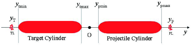
Figure 1: (Color online) Schematic sketch of the distribution of emission sources in rapidity space.

Secondly, we briefly describe the geometrical picture of high-energy collisions. In the multisource thermal model [18, 21] and nuclear geometry theory, a projectile cylinder and a target cylinder are produced at $y$ space when the projectile and target pass each other. In the laboratory reference system or center of mass, we assume that the projectile cylinder is in the positive rapidity direction and the target cylinder is in the negative one, with rapidity ranges [$y_{pmin}$, $y_{pmax}$] and [$y_{tmin}$, $y_{tmax}$], respectively. The projectile and target cylinder are composed of a series of isotropic emission sources with different rapidity shifts. On both sides of the two cylinders, there are leading particles appearing as two isotropic emission sources with rapidity shifts $y_{P}$ and $y_{T}$, respectively. A thick double-cylinder is formed in nucleus-nucleus collisions, and a thin double-cylinder is formed in nucleon-nucleon collisions. With the increasing direction of the rapidity coordinate scalar, we divide the collision system into four parts, the target leading particles (TL), target cylinder (TC), projectile cylinder (PC), and projectile leading particles (PL), respectively. To give a clear picture for understanding the definitions of the variables and parts, different rapidity shifts for different parts in rapidity space are roughly shown in Fig. 1. The two cylinders may overlap completely or overlap partly or may be separated. It is expected that the collision energy corresponding to the situation of separation is higher than that of overlap. The cylinder is not really a specific shape, but it may be understood to be a range of the rapidity of emission sources.

The normalized rapidity distribution can be written as

$$f(y) = k_{t}f(y,y_{T})+\frac{K_{t}}{y_{tmax}-y_{tmin}}\int^{y_{tmax}}_{y_{tmin}}f(y,y_{t})d{y_{t}}$$ (6)

$$+\frac{K_{p}}{y_{pmax}-y_{pmin}}\int^{y_{pmax}}_{y_{pmin}}f(y,y_{p})d{y_{p}}+k_{p}f(y,y_{P}).$$

where $k_{t}$, $K_{t}$, $K_{p}$ and $k_{p}$ are the contributions of TL, TC, PC, and PL, respectively. $y_{p}$ and $y_{t}$ denote the locations of the emission sources in the TC and PC at $y$ space, respectively. For symmetric collisions, $K_{t}=K_{p}=k$, $k_{t}=k_{p}=(1-2k)/2$, $y_{pmax}=-y_{tmin}$, and $y_{pmin}=-y_{tmax}$, the normalized rapidity distribution is rewritten as

$$f(y) = \frac{k}{y_{pmax}-y_{pmin}}\left[\int^{y_{pmax}}_{y_{pmin}}f(y,y_{p})d{y_{p}}+\int^{-y_{pmin}}_{-y_{pmax}}f(y,y_{t})d{y_{t}}\right]$$ (7)

$$+\frac{(1-2k)}{2}\left[f(y,y_{P})+f(y,-y_{P})\right].$$

In the present work, the Monte Carlo method is used to calculate the rapidity distribution. According to the different contribution ratios, the emission sources distribute randomly in the PC range [$y_{pmin}$, $y_{pmax}$], TC range [$y_{tmin}$, $y_{tmax}$], PL region, or TL region. In the final state, the rapidities of particles produced in the two cylinders are given by

$$y_{PC}=(y_{pmax}-y_{pmin})R_{1}+y_{pmin}+y^{\prime},$$

$$y_{TC}=(y_{pmax}-y_{pmin})R_{2}-y_{pmax}+y^{\prime},$$ (8)

where $R_{1}$ and $R_{2}$ are random variables in interval [0,1]. The rapidities of leading particles are

$$y_{PL}=y_{P}+y^{\prime},$$

$$y_{TL}=-y_{P}+y^{\prime}.$$ (9)

In the above expressions, $y^{\prime}$ is calculated by using the Monte Carlo calculation of Eq. (4). In the case of $P_{T}>>m_{0}$, the rapidity $y$ and pseudorapidity $\eta$ are approximately equal to each other. But, the condition of $P_{T}>>m_{0}$ is not always satisfied. A conversion between the pseudorapidity distribution $\frac{dN}{d\eta}$ and the rapidity distribution $\frac{dN}{dy}$ is

$$\frac{dN}{d\eta}=\frac{P}{E}\frac{dN}{dy}=J(\eta,\langle m\rangle/\langle p_{T}\rangle)\frac{dN}{dy}\,\,\,\,,$$ (10)

where a Jacobian of the transformation is

$$J(\eta,\langle m\rangle/\langle P_{T}\rangle)=\frac{\cosh{\eta}}{\sqrt{1+(\langle m\rangle/\langle P_{T}\rangle)^{2}+\sinh^{2}{\eta}}}\,\,\,\,.$$ (11)

3 COMPARISON WITH EXPERIMENTAL RESULTS

3.1 Proton-(anti)proton collisions

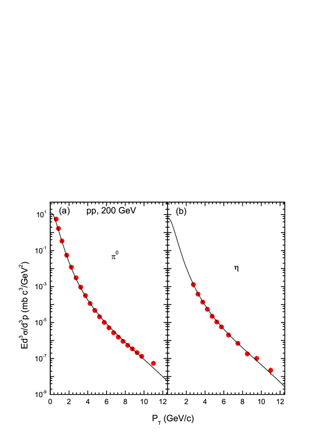
Figure 2: (Color online) Invariant $\pi^{0}$ and $\eta$ cross section as a function of transverse momentum in $pp$ collisions at $\sqrt{\mathrm{\it s_{NN}}}$ = 200 GeV. Experimental data from the PHENIX Collaboration [22, 23] are shown by the scattered symbols. Our calculated results are shown by the curves.

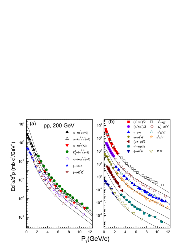
Figure 3: (Color online) Invariant differential cross section of different particles measured in $pp$ collisions at $\sqrt{\mathrm{\it s_{NN}}}$ = 200 GeV in various decay modes. Experimental data measured by the PHENIX Collaboration [10] are shown by the scattered symbols. The curves are our calculated results.

To identify the validity of the model and fix the temperature $T$ and the $q$, Figs. 2 and 3 show invariant yields of final-state particles produced in inelastic (INEL) $pp$ collisions at center-of-mass energy (per nucleon pair) $\sqrt{\mathrm{\it s_{NN}}}=200$ GeV. The symbols are the experimental data of the PHENIX Collaboration [22, 23, 10]. The solid lines are the results calculated by the improved Tsallis distribution. The maximum value of the observed $P_{T}$ reaches about 12.0 GeV/$c$. It can be seen that the results agree well with the experimental data in the region. The $\chi^{2}$ per degree of freedom ($\chi^{2}/{\rm dof}$) testing provides statistical indication of the most probable value of corresponding parameters. The maximum value is 1.210, and the minimum value is 0.324. The parameter values are given in Table I. The parameters $T$ and $q$ are likely stable to be constant values because of the scaling properties of the transverse momentum.

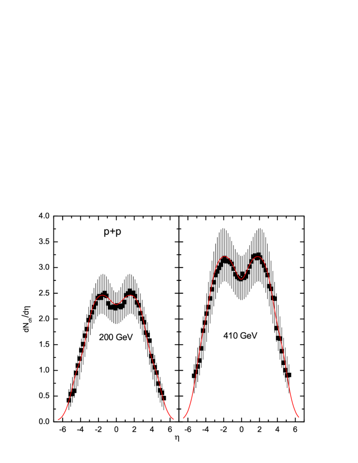
Figure 4: (Color online) The charged particle multiplicity $dN_{ch}/d\eta$ in $pp$ inelastic collisions at $\sqrt{\mathrm{\it s_{NN}}}$ = 200 GeV and 410 GeV. The symbols represent the experimental data of the PHOBOS Collaboration [24]. The curves are our calculated results.

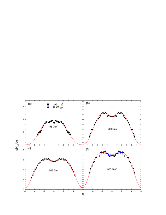
Figure 5: (Color online) The charged particle multiplicity $dN_{ch}/d\eta$ at $\sqrt{\mathrm{\it s_{NN}}}$ = 53, 200, 546 and 900 GeV. The symbols represent the measured data from the UA5 Collaboration [25] ($p\overline{p}$ collisions, with statistical errors only) and the ALICE Collaboration [26] ($pp$ collisions, with statistical errors only). The curves are our calculated results.

Figure 4 shows the pseudorapidity distributions of charged particles produced in INEL $pp$ collisions at $\sqrt{\mathrm{\it s_{NN}}}=200$ and $410$ GeV with $|\eta|$ ranging from 0.10 to 5.30. The solid circles with the error bars represent the experimental data measured by the PHOBOS Collaboration [24]. The solid lines are our results, which are in good agreement with the experimental data. Figure 5 shows the pseudorapidity distributions of charged particles produced in INEL $pp$ (or $p\overline{p}$) collisions at $\sqrt{\mathrm{\it s_{NN}}}=53$, 200, 546, and 900 GeV. The results are compared with measurements made by the UA5 and ALICE collaborations [25, 26]. The corresponding parameter values obtained by fitting the experimental data are given in Table II with $\chi^{2}/{\rm dof}$. From the values, it is found that the $y_{pmax}$ ($-y_{tmin}$), $y_{pmin}$ ($-y_{tmax}$) and $y_{P}$ ($-y_{T}$) increase with increasing the collision energy. So, the gap between the two cylinders and the length of each cylinder also increase with increasing the collision energy. The parameter $k$ does not change obviously, which means that the leading particle contribution is almost identical. From the comparisons, we can see that the multisource thermal model can describe the pseudorapidity distributions of charged particles produced in INEL $pp$ (or $p\overline{p}$) collisions over an energy range from 53 to 900 GeV by using three rapidity shifts $y_{pmin}$, $y_{pmax}$ and $y_{P}$ as free parameters.

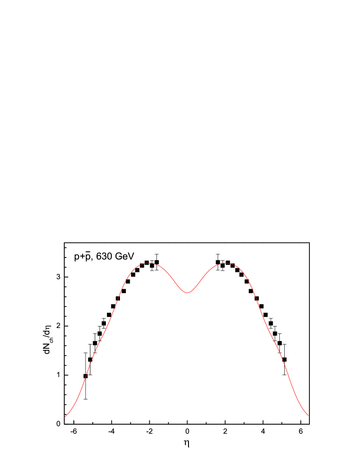
Figure 6: (Color online) The charged particle multiplicity $dN_{ch}/d\eta$ in $p\overline{p}$ inelastic collisions at $\sqrt{\mathrm{\it s_{NN}}}$ = 630 GeV. The symbols and curve represent the same meanings as those in Fig. 5, but the experimental data are taken from the P238 Collaboration [27].

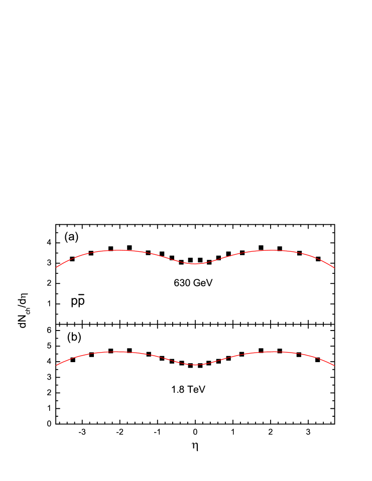
Figure 7: (Color online) The charged particle multiplicity $dN_{ch}/d\eta$ in $p\overline{p}$ inelastic collisions at $\sqrt{\mathrm{\it s_{NN}}}$ = 630 GeV and 1.8 TeV. The symbols and curves represent the same meanings as those in Fig. 5, but the experimental data are taken from the CDF Collaboration [28].

The pseudorapidity distribution of charged particles produced in INEL $p\overline{p}$ collisions at $\sqrt{\mathrm{\it s_{NN}}}=630$ GeV is presented in Fig. 6. The experimental data are measured by the P238 Collaboration [27]. The range of $|\eta|$ is $1.5-5.5$. The parameter values taken in the calculation are given in Table II with $\chi^{2}/{\rm dof}$. One can see that the multisource thermal model with the three free parameters describes the pseudorapidity distribution of charged particles produced in INEL $p\overline{p}$ collisions at $\sqrt{\mathrm{\it s_{NN}}}=630$ GeV, which is higher than RHIC energies and less than LHC energies. Figure 7 shows the pseudorapidity distributions of charged particles produced in INEL $p\overline{p}$ collisions at $\sqrt{\mathrm{\it s_{NN}}}$=630 and 1800 GeV with $|\eta|$ ranging from 0 to 3.5. The experimental data are measured by the CDF Collaboration [28]. By fitting the data, the obtained parameters are given in Table II with $\chi^{2}/{\rm dof}$. The multisource thermal model can also describe the pseudorapidity distribution of charged particles produced in INEL $p\overline{p}$ collisions at $\sqrt{\mathrm{\it s_{NN}}}=630$ and 1800 GeV.

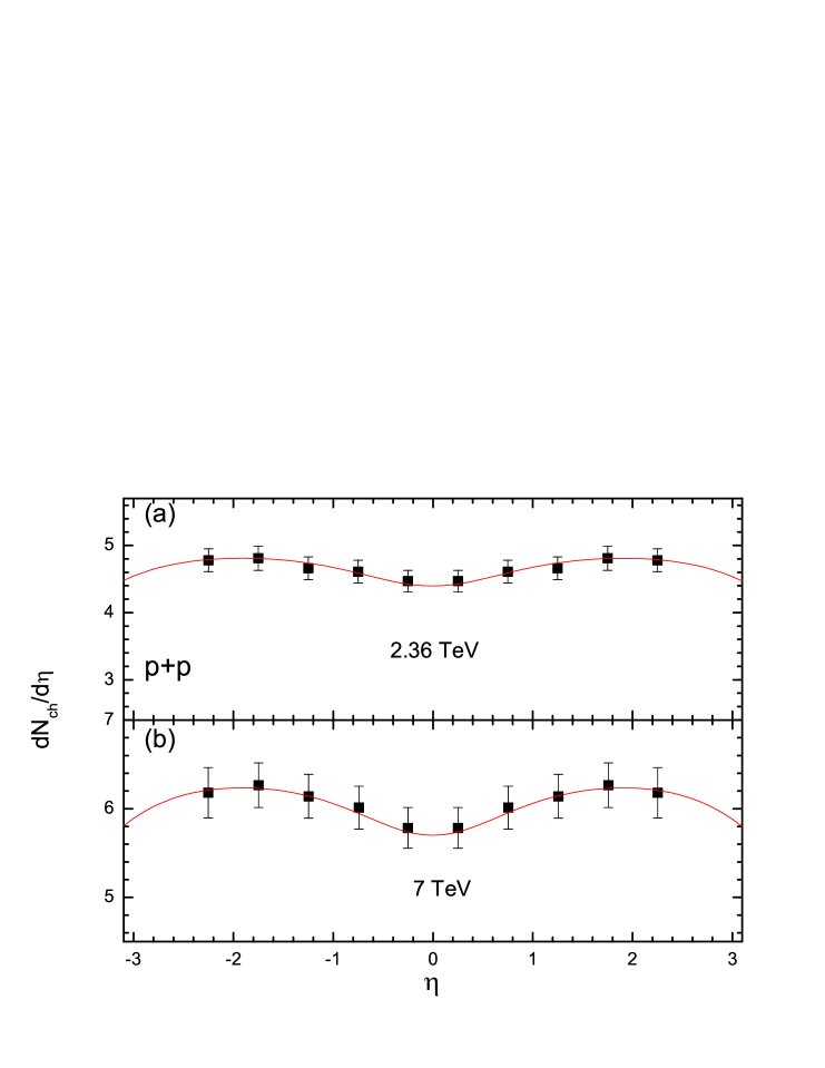
Figure 8: (Color online) The charged particle multiplicity $dN_{ch}/d\eta$ in $pp$ inelastic collisions at $\sqrt{\mathrm{\it s_{NN}}}=$2.36 TeV and 7 TeV. The symbols and curves represent the same meanings as those in Fig. 5, but the experimental data are taken from the CMS Collaboration [15].

For LHC energies, we present the pseudorapidity distributions of charged particles produced in INEL $pp$ collisions at $\sqrt{\mathrm{\it s_{NN}}}$=2.76 and 7 TeV with $|\eta|$ ranging from 0.25 to 2.25 in Fig. 8. The experimental data are measured by the CMS Collaboration [15]. The obtained parameters are given in Table II with $\chi^{2}/{\rm dof}$. Our results are also in good agreement with the data.

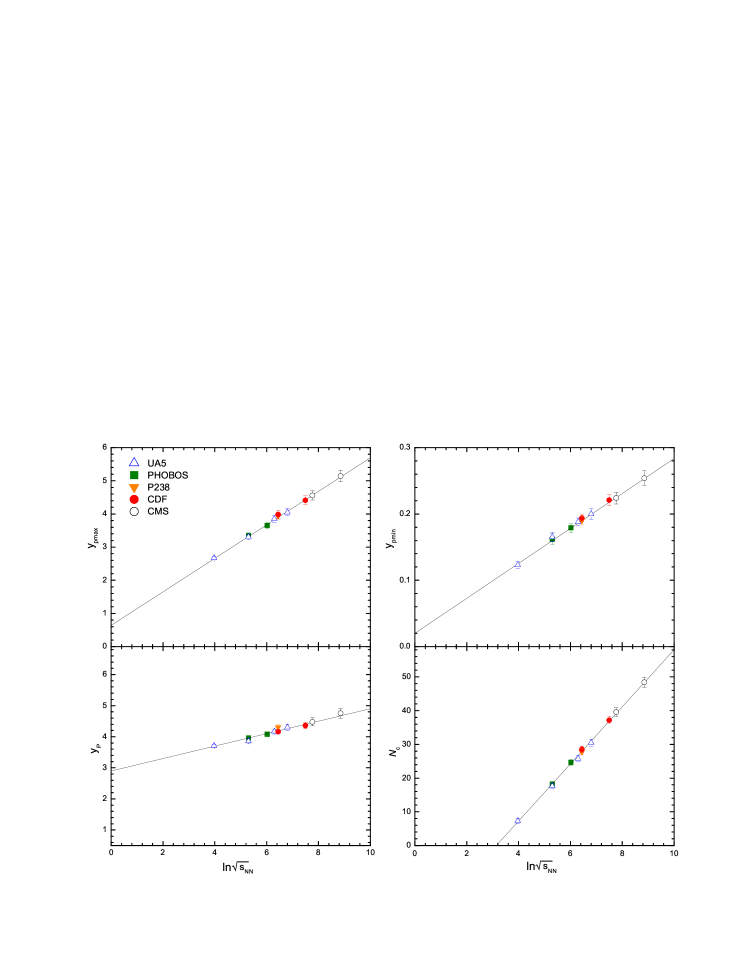
Figure 9: (Color online) The dependence of the different parameters on $\ln{\sqrt{\mathrm{\it s_{NN}}}}$. The symbols represent the parameter values used in the calculations for different experimental collaborations. The solid lines denote the fitted results.

From Table II, it is found that the three parameters obtained by the comparison exhibit the linear dependences on ln$\sqrt{\mathrm{\it s_{NN}}}$. They are given in Fig. 9. The symbols denote the parameters of different collaborations as marked in the figure. The solid lines denote the fitted results, i. e., $y_{pmin}=-y_{tmax}=(0.026\pm 0.004)$ln$\sqrt{\mathrm{\it s_{NN}}}$$+(0.020\pm 0.011)$, $y_{pmax}=-y_{tmin}=(0.506\pm 0.041)$ln$\sqrt{\mathrm{\it s_{NN}}}$$+(0.642\pm 0.061)$ and $y_{P}=-y_{T}=(0.211\pm 0.047)$ln$\sqrt{\mathrm{\it s_{NN}}}$$+(2.855\pm 0.645)$. There is also a linear relationship between the normalization coefficient $N_{c}$ and ln$\sqrt{\mathrm{\it s_{NN}}}$, $N_{c}=(8.469\pm 0.032)$ln$\sqrt{\mathrm{\it s_{NN}}}$$-(26.788\pm 1.570)$. The $\chi^{2}/{\rm dof}$ are 0.012, 0.040, 0.029 and 0.021, respectively. According to the linear laws, the values of the parameters used in the model for $pp$($p\overline{p}$) collisions at higher energies can be predicted. Then, we may predict the pseudorapidity distributions of charged particles produced at LHC energies. When $\sqrt{\mathrm{\it s_{NN}}}$ rises up to 10 and 14 TeV, the parameters are taken to be $y_{pmin}=$ 0.260 and 0.271, $y_{pmax}$=5.297 and 5.471, $y_{P}$=4.798 and 4.862, and $N_{c}$=51.280 and 54.204. The prediction of the pseudorapidity distribution are given in Fig. 10.

3.2 Nucleus-nucleus collisions

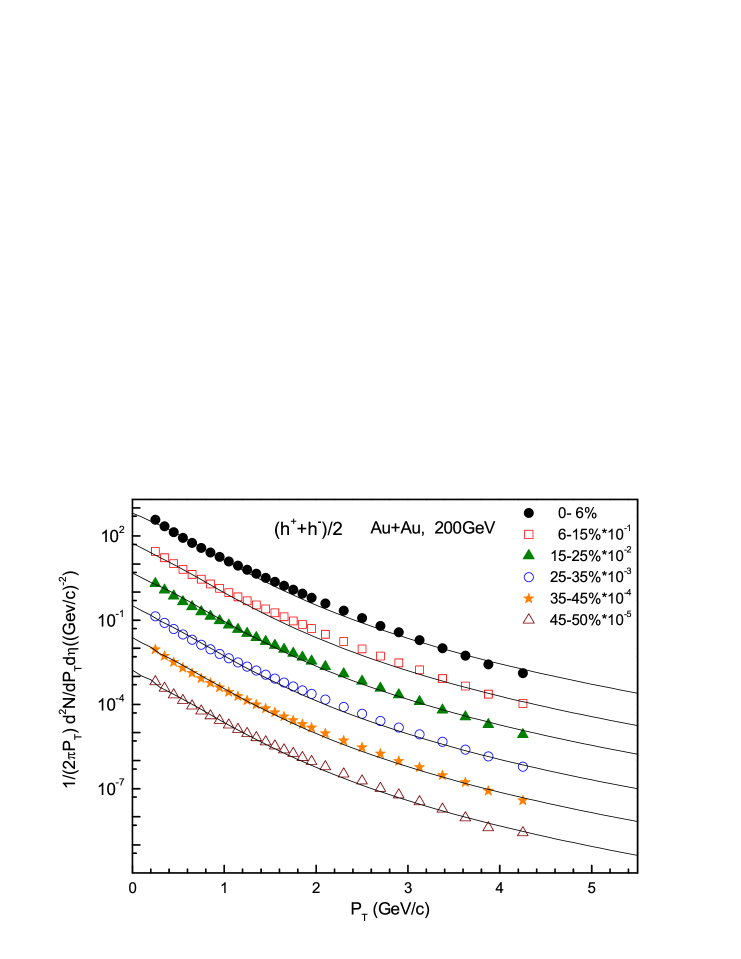
Figure 11: (Color online) Charged hadron transverse momentum distributions in Au+Au collisions at $\sqrt{\mathrm{\it s_{NN}}}$ =200 GeV. For clarity, consecutive bins are scaled by factors of 10. Experimental data of the PHOBOS Collaboration [29] are shown by the scattered symbols. Our calculated results are shown by the curves.

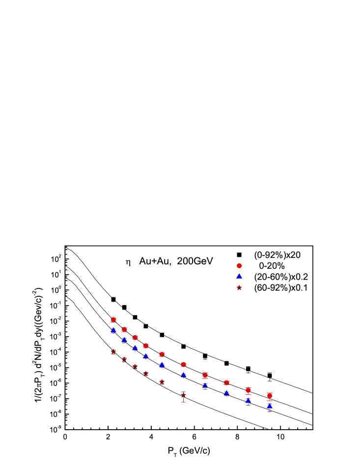
Figure 12: (Color online) $\eta$ transverse momentum distributions in Au+Au collisions at $\sqrt{\mathrm{\it s_{NN}}}$ = 200 GeV. The error bars are the quadratic sum of statistical and systematic uncertainties. Experimental data of the PHENIX Collaboration [30] are shown by the scattered symbols. Our calculated results are shown by the curves.

Figures 11 and 12 show the $P_{T}$ spectra of charged hadrons and $\eta$ particles for the different centralities in Au+Au collisions at $\sqrt{\mathrm{\it s_{NN}}}=200$ GeV with $|\eta|$ ranging from 0.1 to 5.3. The symbols are the experimental data from the PHOBOS Collaboration [29] and the PHENIX Collaboration [30]. The solid lines are the results fitted by the improved Tsallis distribution. The parameter values are given in Table III with $\chi^{2}/{\rm dof}$. Because the scaling properties of the transverse momentum, the values of $T$ and $q$ do not change significantly with the centralities. The maximum value of $\chi^{2}/{\rm dof}$ is 0.671, and the minimum value is 0.358.

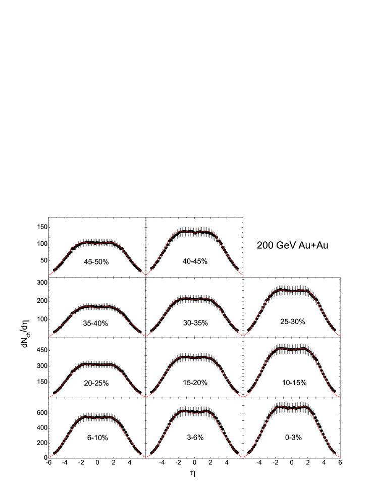
Figure 13: (Color online) The charged particle multiplicity $dN_{ch}/d\eta$ for different centrality bins in Au+Au collisions at $\sqrt{\mathrm{\it s_{NN}}}$ = 200 GeV. Experimental data of the PHOBOS Collaboration [24] are shown by the scattered symbols. Our calculated results are shown by the curves.

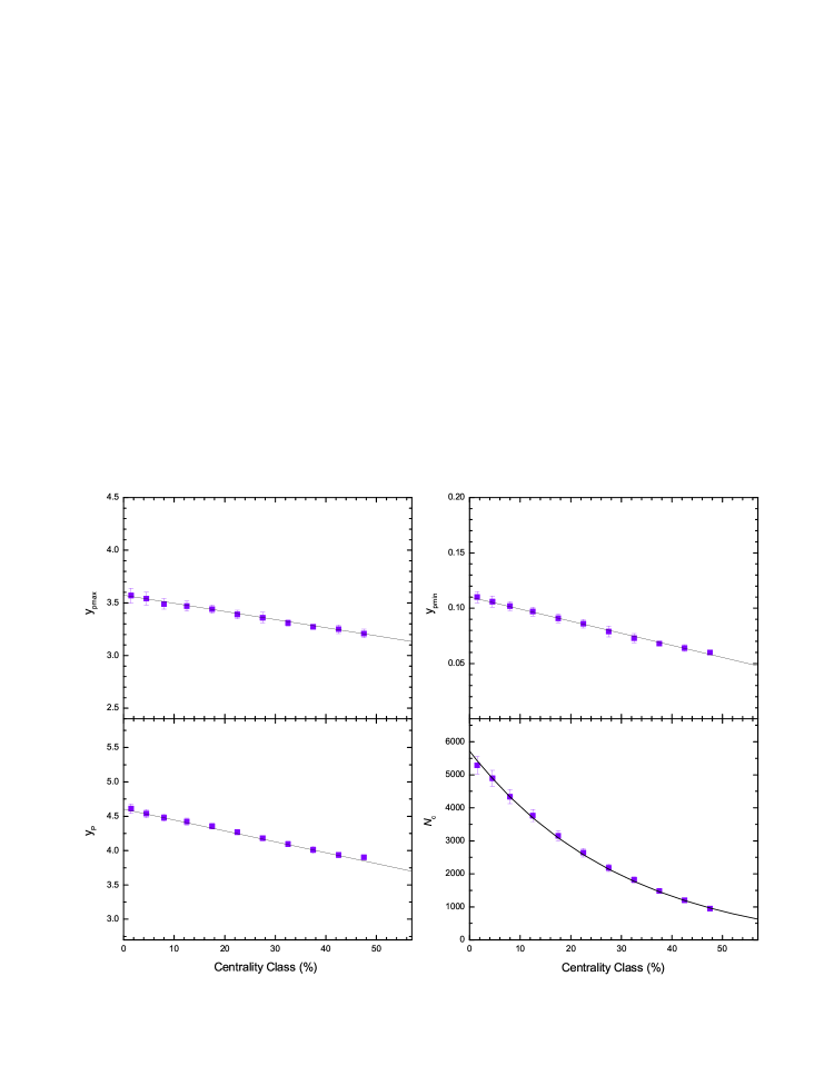
Figure 14: (Color online) The dependence of the parameters on the centrality class. The symbols represent the values used in the calculations of Fig. 13. The lines are fitted results.

The pseudorapidity distributions of charged particles for eleven centrality bins in Au+Au collisions at $\sqrt{\mathrm{\it s_{NN}}}=200$ GeV are presented in Fig. 13. The symbols with the error bars denote the experimental data of the PHOBOS Collaboration [24]. The solid lines denote our results. In the calculation, the parameters used in the calculation are given in Table IV with $\chi^{2}/{\rm dof}$. The $y_{pmax}$ ($-y_{tmin}$), $y_{pmin}$ ($-y_{tmax}$) and $y_{P}$ ($-y_{T}$) increase linearly with increasing the centrality or decrease linearly with increasing the centrality percentage $C$. They are plotted in Fig. 14, where the solid lines are the fitted results $y_{pmin}=-y_{tmax}=-0.001$$C$$+(0.110\pm 0.021)$, $y_{pmax}=-y_{tmin}=-(0.008\pm 0.001)$$C$$+(3.574\pm 0.042)$, and $y_{P}=-y_{T}=-(0.016\pm 0.002)$$C$$+(4.604\pm 0.049)$. The normalization coefficient is

$$N_{c}=(6020.5\pm 37.5)\exp{(-\frac{C}{0.305\pm 0.006})}-(300.5\pm 71.5).$$ (12)

According to the laws, the pseudorapidity distributions of charged particles for other centralities may be predicted.

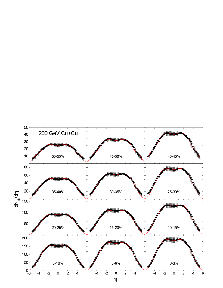
Figure 15: (Color online) Same as for Fig. 13, but for Cu+Cu collisions.

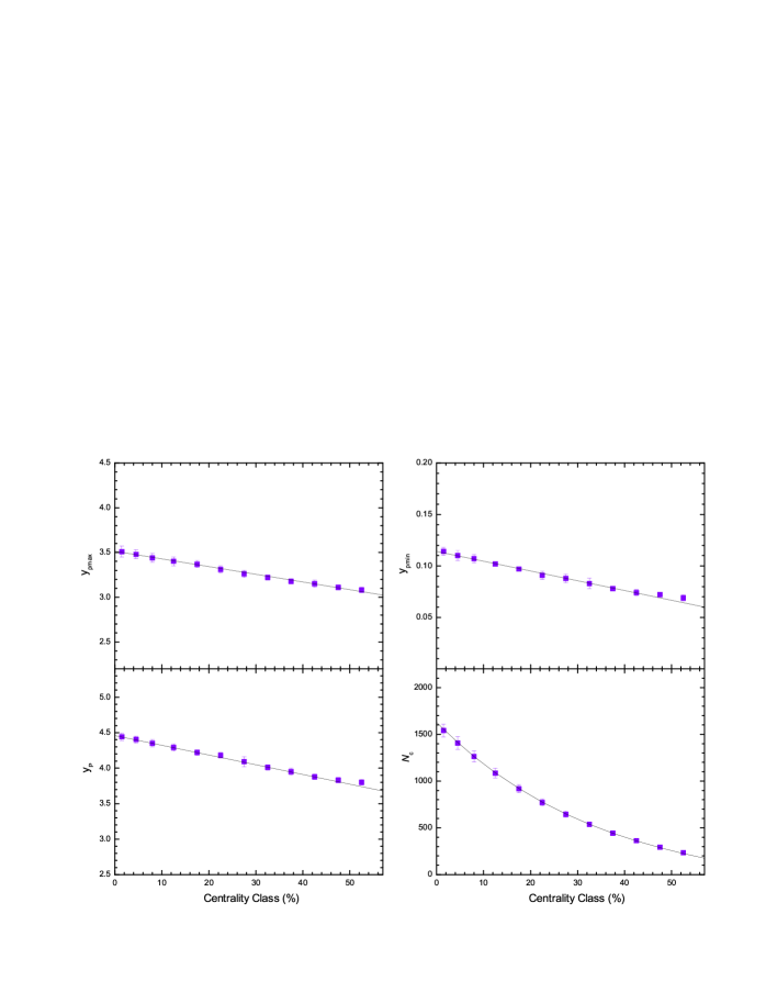
Figure 16: (Color online) Same as Fig. 14, but for the parameters used in Fig. 15.

Figure 15 shows the pseudorapidity distributions of charged particles for twelve centrality bins in Cu+Cu collisions at $\sqrt{\mathrm{\it s_{NN}}}=200$ GeV. The symbols and lines represent the same meanings as those in Fig. 13. Our results are also in good agreement with the experimental data. The parameters are given in Table IV with $\chi^{2}/{\rm dof}$. By fitting the parameters, the obtained relationships between the parameters and $C$ are $y_{pmin}=-y_{tmax}=-0.001$$C$$+(0.115\pm 0.006)$, $y_{pmax}=-y_{tmin}=-(0.009\pm 0.001)$$C$$+(3.514\pm 0.039)$, $y_{P}=-y_{T}=-(0.014\pm 0.002)$$C$$+(4.460\pm 0.055)$, and the normalization coefficient is $N_{c}=(1820.7\pm 11.5)\exp{(-\frac{C}{0.355\pm 0.005})}-(190.5\pm 39.5)$ as given in Fig. 16.

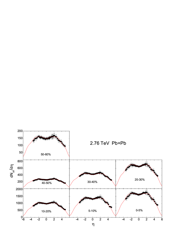
Figure 17: (Color online)The charged particle multiplicity $dN_{ch}/d\eta$ for different centrality bins in Pb+Pb collisions at $\sqrt{\mathrm{\it s_{NN}}}$ = 2.76 TeV. Experimental data of the ALICE Collaboration [31] are shown by the scattered symbols. Our calculated results are shown by the curves.

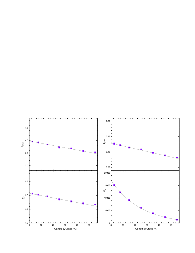
Figure 18: (Color online) Same as Fig. 14, but for the parameters used in Fig. 17.

Figure 17 shows the pseudorapidity distributions of charged particles for seven centrality bins in Pb+Pb collisions at $\sqrt{\mathrm{\it s_{NN}}}=2.76$ TeV. The symbols with the error bars are the experimental data measured at the LHC [31]. The solid lines are our results. From the figure, we know that the multisource thermal model with the three free parameters can also describe the pseudorapidity distributions of charged particles produced in Pb+Pb collisions at $\sqrt{\mathrm{\it s_{NN}}}=2.76$ TeV. The parameter values are given in Table IV with $\chi^{2}/{\rm dof}$. The parameters as the function of $C$ are $y_{pmin}=-y_{tmax}=-0.001$$C$$+(0.129\pm 0.007)$, $y_{pmax}=-y_{tmin}=-(0.009\pm 0.001)$$C$$+(3.982\pm 0.045)$, $y_{P}=-y_{T}=-(0.010\pm 0.002)$$C$$+(5.080\pm 0.057)$, and the normalization coefficient is $N_{c}=(17580.5\pm 104.4)\exp{(-\frac{C}{0.251\pm 0.004})}-(600.5\pm 112.5)$ as given in Fig. 18.

4 CONCLUSIONS

We embed consistently the improved form of the Tsallis distribution into the multisource thermal model for describing hadron productions in $pp$ (or $p\overline{p}$) and $AA$ collisions at RHIC and LHC energies. The pseudorapidity distributions have been systematically investigated and compared to the experimental data for $pp$($\overline{p}$) and Au+Au, Cu+Cu, and Pb+Pb collisions at the RHIC and LHC energies. The updated multisource thermal model can describe the experimental results. The three free parameters $y_{pmax}$ ($-y_{tmin}$), $y_{pmin}=-y_{tmax}$, and $y_{P}$ (-$y_{T}$) taken in the calculations exhibit certain regularities for the collision energy and the collision centrality. The linear dependences of the parameters on ln$\sqrt{\mathrm{\it s_{NN}}}$ are found. It may be used to predict the pseudorapidity distributions of produced particles in $pp$($\overline{p}$) at higher colliding energies such as LHC energies. And it is also used to predict the pseudorapidity distributions of produced particles in Au+Au, Cu+Cu, and Pb+Pb collisions with other centralities at high energies. As an example, we have given the predictions of the pseudorapidity distributions of charged particles produced in $pp$($\overline{p}$) collisions at higher energies.

The multisource thermal model was developed by us in the past years [18, 21]. This model assumes that many emission sources of produced particles and nuclear fragments are formed in high-energy collisions. The particles are emitted isotropically in the rest frame of the emission sources with the different excitation degree in collisions. Each emission source was treated as a thermal equilibrium system of classical ideal gas. So, the classical Maxwell s ideal gas distribution was adopted without considering the effects of the relativity and quantum. Recently, the improved Tsallis distribution [19] was suggested in the particular case of relativistic high-energy quantum distributions. Moreover, the thermodynamic consistency of the distribution was considered in detail. The temperature $T$ and the degree of nonequilibrium $q$ can be determined by a global fit of the $P_{T}$ spectra. In the present work, we combined the improved Tsallis distribution and the picture of the multisource thermal model. The pseudorapidity distributions are mainly related to the rapidity of the emission sources in the formalism.

In summary, the pseudorapidity distributions of charged particles produced in nucleus-nucleus and nucleon-nucleon collisions at RHIC and LHC energies have been studied in the improved multisource thermal model, where the improved Tsallis distribution is embedded. The results in each collision are compared with experimental data measured by different collaborations. Our investigations indicate the improved model is successful in the description of hadron productions. At the same time, it is found that the rapidity shifts of the two cylinders are linearly related to ln$\sqrt{\mathrm{\it s_{NN}}}$. According to the laws, the predictions of the results at higher-energy collisions are given.

Acknowledgments. This work is supported by the National Natural Science Foundation of China under Grants No. 11247250, No. 11005071, and No. 10975095; the National Fundamental Fund of Personnel Training under Grant No. J1103210, the Shanxi Provincial Natural Science Foundation under Grants No. 2013021006 and No. 2011011001; the Open Research Subject of the Chinese Academy of Sciences Large-Scale Scientific Facility under Grant No. 2060205, and the Shanxi Scholarship Council of China.

Table 1: Parameter values corresponding to the solid curves in Fig. 2 and Fig. 3.

Figure	Collision	Particle	$T$ (GeV)	$q$	$\chi^{2}$/dof
2(a)	$pp$	$\pi^{0}$	$0.047\pm 0.005$	$1.077\pm 0.015$	$0.324$
2(b)	$pp$	$\eta$	$0.047\pm 0.005$	$1.082\pm 0.010$	$0.390$
3(a)	$p\overline{p}$	$\omega$	$0.047\pm 0.005$	$1.082\pm 0.012$	$1.210$
	$p\overline{p}$	$K_{s}^{0}$	$0.047\pm 0.005$	$1.078\pm 0.015$	$0.675$
	$pp$	$\eta^{\prime}$	$0.047\pm 0.005$	$1.082\pm 0.010$	$0.624$
	$pp$	$\phi$	$0.047\pm 0.005$	$1.082\pm 0.009$	$0.647$
3(b)	$p\overline{p}$	$\pi$	$0.050\pm 0.005$	$1.079\pm 0.012$	$0.546$
	$p\overline{p}$	$K$	$0.050\pm 0.005$	$1.079\pm 0.010$	$0.575$
	$p\overline{p}$	$\eta$	$0.050\pm 0.005$	$1.079\pm 0.010$	$0.951$
	$p\overline{p}$	$\omega$	$0.050\pm 0.005$	$1.082\pm 0.015$	$0.744$
	$p\overline{p}$	$p(\overline{p})$	$0.050\pm 0.005$	$1.082\pm 0.015$	$0.524$
	$pp$	$\eta^{\prime}$	$0.050\pm 0.005$	$1.082\pm 0.012$	$0.803$
	$pp$	$\phi$	$0.050\pm 0.005$	$1.082\pm 0.012$	$1.112$

Table 2: Parameter values corresponding to the solid curves in Figs. 4-8.

Figure	Energy (GeV)	Collision	$y_{pmax}$	$y_{pmin}$	$y_{P}$	$k$	$N_{c}$	$\chi^{2}$/dof
4(a)	200	$pp$	$3.35\pm 0.08$	$0.162\pm 0.008$	$3.94\pm 0.08$	$0.432\pm 0.010$	$18.20\pm 0.85$	$0.915$
4(b)	410	$pp$	$3.65\pm 0.09$	$0.179\pm 0.007$	$4.08\pm 0.07$	$0.432\pm 0.010$	$24.65\pm 0.94$	$0.726$
5(a)	53	$p\overline{p}$	$2.67\pm 0.05$	$0.123\pm 0.005$	$3.71\pm 0.05$	$0.432\pm 0.010$	$7.24\pm 0.70$	$1.127$
5(b)	200	$p\overline{p}$	$3.31\pm 0.07$	$0.165\pm 0.007$	$3.88\pm 0.07$	$0.432\pm 0.010$	$17.60\pm 0.75$	$0.958$
5(c)	546	$p\overline{p}$	$3.85\pm 0.10$	$0.188\pm 0.006$	$4.17\pm 0.08$	$0.432\pm 0.010$	$25.80\pm 0.91$	$0.549$
5(d)	900	$pp$ and $p\overline{p}$	$4.05\pm 0.11$	$0.200\pm 0.008$	$4.30\pm 0.09$	$0.432\pm 0.010$	$30.50\pm 1.05$	$0.752$
6	630	$p\overline{p}$	$3.94\pm 0.10$	$0.192\pm 0.005$	$4.29\pm 0.08$	$0.432\pm 0.010$	$27.80\pm 0.95$	$1.265$
7(a)	630	$p\overline{p}$	$3.99\pm 0.12$	$0.194\pm 0.006$	$4.16\pm 0.06$	$0.432\pm 0.010$	$28.50\pm 1.00$	$0.650$
7(b)	900	$p\overline{p}$	$4.41\pm 0.13$	$0.221\pm 0.008$	$4.36\pm 0.10$	$0.432\pm 0.010$	$37.20\pm 1.15$	$0.461$
8(a)	2360	$pp$	$4.56\pm 0.14$	$0.225\pm 0.009$	$4.48\pm 0.12$	$0.432\pm 0.010$	$39.56\pm 1.24$	$0.650$
8(b)	7000	$pp$	$5.15\pm 0.15$	$0.254\pm 0.011$	$4.76\pm 0.14$	$0.432\pm 0.010$	$48.46\pm 1.47$	$0.461$

Table 3: Parameter values corresponding to the solid curves in Fig. 11 and Fig. 12.

Figure	Centrality	$T$ (GeV)	$q$	$\chi^{2}$/dof
11	$0-6\%$	$0.065\pm 0.005$	$1.069\pm 0.004$	$0.502$
	$6-15\%$	$0.065\pm 0.005$	$1.069\pm 0.004$	$0.655$
	$15-25\%$	$0.065\pm 0.005$	$1.069\pm 0.004$	$0.618$
	$25-35\%$	$0.065\pm 0.005$	$1.069\pm 0.004$	$0.560$
	$35-45\%$	$0.065\pm 0.005$	$1.069\pm 0.004$	$0.582$
	$45-50\%$	$0.065\pm 0.005$	$1.069\pm 0.004$	$0.671$
12	$0-20\%$	$0.060\pm 0.005$	$1.074\pm 0.005$	$0.358$
	$20-60\%$	$0.060\pm 0.005$	$1.074\pm 0.005$	$0.470$
	$60-92\%$	$0.060\pm 0.005$	$1.074\pm 0.005$	$0.502$
	$0-92\%$	$0.060\pm 0.005$	$1.074\pm 0.005$	$0.516$

Table 4: Parameter values corresponding to the solid curves in Fig. 13, Fig. 15 and Fig. 17.

Figure	Collision	Centrality	$y_{pmax}$	$y_{pmin}$	$y_{P}$	$k$	$Nc$	$\chi^{2}$/dof
13	Au+Au	$0-3\%$	$3.57\pm 0.07$	$0.110\pm 0.005$	$4.61\pm 0.07$	$0.430\pm 0.005$	$5290\pm 264$	$0.550$
		$3-6\%$	$3.54\pm 0.06$	$0.106\pm 0.005$	$4.54\pm 0.06$	$0.430\pm 0.005$	$4895\pm 245$	$0.652$
		$6-10\%$	$3.49\pm 0.05$	$0.102\pm 0.004$	$4.48\pm 0.05$	$0.430\pm 0.005$	$4341\pm 217$	$0.484$
		$10-15\%$	$3.47\pm 0.05$	$0.097\pm 0.004$	$4.42\pm 0.05$	$0.430\pm 0.005$	$3763\pm 188$	$0.426$
		$15-20\%$	$3.44\pm 0.04$	$0.091\pm 0.004$	$4.36\pm 0.04$	$0.430\pm 0.005$	$3153\pm 158$	$0.424$
		$20-25\%$	$3.39\pm 0.04$	$0.086\pm 0.004$	$4.27\pm 0.04$	$0.430\pm 0.005$	$2645\pm 132$	$0.427$
		$25-30\%$	$3.36\pm 0.05$	$0.079\pm 0.005$	$4.18\pm 0.04$	$0.430\pm 0.005$	$2184\pm 109$	$0.520$
		$30-35\%$	$3.31\pm 0.03$	$0.073\pm 0.004$	$4.10\pm 0.04$	$0.427\pm 0.005$	$1819\pm 91$	$0.576$
		$35-40\%$	$3.27\pm 0.02$	$0.068\pm 0.002$	$4.01\pm 0.05$	$0.427\pm 0.005$	$1486\pm 74$	$0.583$
		$40-45\%$	$3.25\pm 0.04$	$0.064\pm 0.003$	$3.94\pm 0.04$	$0.427\pm 0.005$	$1204\pm 60$	$0.658$
		$45-50\%$	$3.21\pm 0.04$	$0.060\pm 0.002$	$3.90\pm 0.02$	$0.427\pm 0.005$	$951\pm 48$	$0.642$
15	Cu+Cu	$0-3\%$	$3.51\pm 0.06$	$0.114\pm 0.004$	$4.45\pm 0.05$	$0.430\pm 0.005$	$1541\pm 70$	$0.572$
		$3-6\%$	$3.48\pm 0.05$	$0.110\pm 0.005$	$4.40\pm 0.05$	$0.430\pm 0.005$	$1407\pm 68$	$0.645$
		$6-10\%$	$3.44\pm 0.05$	$0.107\pm 0.004$	$4.35\pm 0.05$	$0.430\pm 0.005$	$1262\pm 59$	$0.506$
		$10-15\%$	$3.40\pm 0.05$	$0.102\pm 0.002$	$4.29\pm 0.05$	$0.430\pm 0.005$	$1084\pm 51$	$0.521$
		$15-20\%$	$3.37\pm 0.04$	$0.097\pm 0.002$	$4.22\pm 0.04$	$0.427\pm 0.005$	$917\pm 43$	$0.558$
		$20-25\%$	$3.31\pm 0.04$	$0.091\pm 0.004$	$4.18\pm 0.04$	$0.427\pm 0.005$	$771\pm 38$	$0.515$
		$25-30\%$	$3.26\pm 0.04$	$0.088\pm 0.004$	$4.09\pm 0.06$	$0.427\pm 0.005$	$645\pm 32$	$0.570$
		$30-35\%$	$3.22\pm 0.03$	$0.083\pm 0.005$	$4.01\pm 0.04$	$0.427\pm 0.005$	$538\pm 27$	$0.566$
		$35-40\%$	$3.19\pm 0.03$	$0.078\pm 0.002$	$3.95\pm 0.05$	$0.427\pm 0.005$	$445\pm 23$	$0.562$
		$40-45\%$	$3.15\pm 0.04$	$0.074\pm 0.003$	$3.88\pm 0.04$	$0.425\pm 0.005$	$364\pm 19$	$0.597$
		$45-50\%$	$3.11\pm 0.03$	$0.072\pm 0.002$	$3.83\pm 0.05$	$0.425\pm 0.005$	$293\pm 15$	$0.620$
		$50-55\%$	$3.08\pm 0.03$	$0.070\pm 0.003$	$3.80\pm 0.05$	$0.425\pm 0.005$	$234\pm 13$	$0.625$
17	Pb+Pb	$0-5\%$	$3.96\pm 0.05$	$0.126\pm 0.004$	$5.06\pm 0.04$	$0.422\pm 0.005$	$15200\pm 400$	$0.925$
		$5-10\%$	$3.91\pm 0.04$	$0.123\pm 0.002$	$5.02\pm 0.03$	$0.422\pm 0.005$	$12350\pm 240$	$0.805$
		$10-20\%$	$3.84\pm 0.03$	$0.114\pm 0.004$	$4.97\pm 0.03$	$0.422\pm 0.005$	$9200\pm 180$	$0.778$
		$20-30\%$	$3.75\pm 0.05$	$0.108\pm 0.004$	$4.88\pm 0.04$	$0.419\pm 0.005$	$6080\pm 140$	$1.156$
		$30-40\%$	$3.68\pm 0.04$	$0.096\pm 0.002$	$4.80\pm 0.05$	$0.419\pm 0.005$	$3950\pm 80$	$0.718$
		$40-50\%$	$3.59\pm 0.03$	$0.089\pm 0.003$	$4.72\pm 0.04$	$0.419\pm 0.005$	$2405\pm 68$	$0.627$
		$50-60\%$	$3.53\pm 0.02$	$0.083\pm 0.002$	$4.67\pm 0.02$	$0.419\pm 0.005$	$1340\pm 46$	$0.644$

Figure 10: (Color online) The charged particle multiplicity $dN_{ch}/d\eta$ in $pp$ (or $p\overline{p}$) collisions at $\sqrt{\mathrm{\it s_{NN}}}$ = 10 TeV and 14 TeV.

References

• [1] J.Β Adams et al. [STAR Collaboration], Phys.Β Rev.Β Lett.Β  92, 112301 (2004).
• [2] The CMS Collaboration, CMS-PAS-QCD-08-004.
• [3] B.Β B.Β Abelev et al. [ALICE Collaboration], arXiv:1307.6796 [nucl-ex].
• [4] P.Β Braun-Munzinger et al., Phys.Β Lett.Β B 518, 41 (2001).
• [5] J.Β Rafelski and J.Β Letessier, Nucl.Β Phys.Β A 715, 98 (2003).
• [6] A.Β Andronic, P.Β Braun-Munzinger and J.Β Stachel, Phys.Β Lett.Β B 673, 142 (2009) [Erratum-ibid.Β B 678, 516 (2009)].
• [7] J.Β Cleymans, I.Β Kraus, H.Β Oeschler, K.Β Redlich and S.Β Wheaton, Phys.Β Rev.Β C 74, 034903 (2006).
• [8] P.Β Braun-Munzinger, J.Β Stachel and C.Β Wetterich, Phys.Β Lett.Β B 596, 61 (2004).
• [9] A.Β Adare et al. [PHENIX Collaboration], Phys.Β Rev.Β C 83, 064903 (2011) [arXiv:1102.0753 [nucl-ex]].
• [10] A.Β Adare et al. [PHENIX Collaboration], Phys.Β Rev.Β D 83, 052004 (2011).
• [11] B.Β I.Β Abelev et al. [STAR Collaboration], Phys.Β Rev.Β C 75, 064901 (2007) [nucl-ex/0607033].
• [12] KAamodt et al. [ALICE Collaboration], Phys.Β Lett.Β B 693, 53 (2010) [arXiv:1007.0719 [hep-ex]].
• [13] G.Β Aad et al. [ATLAS Collaboration], New J.Β Phys.Β  13, 053033 (2011) [arXiv:1012.5104 [hep-ex]].
• [14] V.Β Khachatryan et al. [CMS Collaboration], JHEP 1002, 041 (2010) [arXiv:1002.0621 [hep-ex]].
• [15] V.Β Khachatryan et al. [CMS Collaboration], Phys.Β Rev.Β Lett.Β  105, 022002 (2010).
• [16] J.Β Cleymans, G.Β I.Β Lykasov, A.Β S.Β Parvan, A.Β S.Β Sorin, O.Β V.Β Teryaev and D.Β Worku, Phys.Β Lett.Β B 723, 351 (2013) [arXiv:1302.1970 [hep-ph]]; J.Β Cleymans, J.Β Phys.Β Conf.Β Ser.Β  455, 012049 (2013); M.Β D.Β Azmi and J.Β Cleymans, arXiv:1311.2909 [hep-ph]; M.Β D.Β Azmi and J.Β Cleymans, arXiv:1401.4835 [hep-ph].
• [17] C.Β -Y.Β Wong and G.Β Wilk, Phys.Β Rev.Β D 87, 114007 (2013) [arXiv:1305.2627 [hep-ph]]; C.Β -Y.Β Wong and G.Β Wilk, Acta Phys.Β Polon.Β B 43, 2047 (2012) [arXiv:1210.3661 [hep-ph]]; G.Β Wilk and Z.Β Wlodarczyk, Phys.Β Rev.Β Lett.Β  84, 2770 (2000) [hep-ph/9908459].
• [18] B.Β C.Β Li, Y.Β Y.Β Fu, L.Β L.Wang, E.Β Q.Β Wang and F.Β H.Β Liu, J.Β Phys.Β G 39, 025009 (2012).
• [19] J.Β Cleymans and D.Β Worku, Eur.Β Phys.Β J.Β A 48, 160 (2012).
• [20] S.Β -q.Β Feng, F.Β Liu and L.Β -s.Β Liu, Phys.Β Rev.Β C 63, 014901 (2001).
• [21] F.Β -H.Β Liu, N.Β N.Β Abd Allah and B.Β K.Β Singh, Phys.Β Rev.Β C 69, 057601 (2004).
• [22] A.Β Adare et al. [PHENIX Collaboration], Phys.Β Rev.Β Lett.Β  101, 162301 (2008).
• [23] S.Β S.Β Adler et al. [PHENIX Collaboration], Phys.Β Rev.Β Lett.Β  98, 172302 (2007).
• [24] B.Β Alver et al. [PHOBOS Collaboration], Phys.Β Rev.Β C 83, 024913 (2011).
• [25] G.Β J.Β Alner et al. [UA5 Collaboration], Phys.Β Rep.Β  154, 247 (1987).
• [26] K.Β Aamodt et al. [ALICE Collaboration], Eur.Β Phys.Β J.Β C 68, 89 (2010).
• [27] R.Β Harr, C.Β Liapis, P.Β Karchin, C.Β Biino, S.Β Erhan, W.Β Hofmann, P.Β Kreuzer and D.Β Lynn et al., Phys.Β Lett.Β B 401, 176 (1997).
• [28] F.Β Abe et al. [CDF Collaboration], Phys.Β Rev.Β D 41, 2330 (1990).
• [29] B.Β B.Β Back et al. [ PHOBOS Collaboration ], Phys.Β Lett.Β B 578, 297-303 (2004).
• [30] S.Β S.Β Adler et al. [PHENIX Collaboration], Phys.Β Rev.Β Lett.Β  96, 202301 (2006).
• [31] E.Β Abbas et al. [ALICE Collaboration], Phys.Β Lett.Β B 726, 610 (2013).