Measuring Global Similarity between Texts

Abstract

We propose a new similarity measure between texts which, contrary to the current state-of-the-art approaches, takes a global view of the texts to be compared. We have implemented a tool to compute our textual distance and conducted experiments on several corpuses of texts. The experiments show that our methods can reliably identify different global types of texts.

1 Introduction

Statistical approaches for comparing texts are used for example in machine translation for assessing the quality of machine translation tools [22, 18, 19], or in computational linguistics in order to establish authorship [30, 14, 24, 25, 17, 3] or to detect “fake”, i.e., automatically generated, scientific papers [16, 21].

Generally speaking, these approaches consist in computing distances, or similarity measures, between texts and then using statistical methods such as, for instance, hierarchical clustering [10] to organize the distance data and draw conclusions.

The distances between texts which appear to be the most popular, e.g., [14, 22], are all based on measuring differences in $1$-gram frequencies: For each $1$-gram (token, or word) $w$ in the union of $A$ and $B$, its absolute frequencies in both texts are calculated, i.e., $F_{A}(w)$ and $F_{B}(w)$ are the numbers of occurrences of $w$ in $A$ and $B$, respectively, and then the distance between $A$ and $B$ is defined to be the sum, over all words $w$ in the union of $A$ and $B$, of the absolute differences $|F_{A}(w)-F_{B}(w)|$, divided by the combined length of $A$ and $B$ for normalization. When the texts $A$ and $B$ have different length, some adjustments are needed; also, some algorithms [22, 18] take into account also $2$-, $3$- and $4$-grams.

These distances are thus based on a local model of the texts: they measure differences of the multisets of $n$-grams for $n$ between $1$ and maximally $4$. Borrowing techniques from economics and theoretical computer science, we will propose below a new distance which instead builds on the global structure of the texts. It simultaneously measures differences in occurrences of $n$-grams for all $n$ and uses a discounting parameter to balance the influence of long $n$-grams versus short $n$-grams.

Following the example of [16], we then use our distance to automatically identify “fake” scientific papers. These are “papers” which are automatically generated by some piece of software and are hence devoid of any meaning, but which, at first sight, have the appearance of a genuine scientific paper.

We can show that using our distance and hierarchical clustering, we are able to automatically identify such fake papers, also papers generated by other methods than the ones considered in [16], and that, importantly, some parts of the analysis become more reliable the higher the discounting factor. We conclude that measuring global differences between texts, as per our method, can be a more reliable way than the current state-of-the-art methods to automatically identify fake scientific papers. We believe that this also has applications in other areas such machine translation or computational linguistics.

2 Inter-textual Distances

For the purpose of this paper, a text $A$ is a sequence $A=(a_{1},a_{2},\dots,a_{N_{A}})$ of words. The number $N_{A}$ is called the length of $A$. As a vehicle for showing idealized properties, we may sometimes also speak of infinite texts, but most commonly, texts are finite and their length is a natural number. Note that we pay no attention to punctuation, structure such as headings or footnotes, or non-textual parts such as images.

2.1 1-gram distance

Before introducing our global distance, we quickly recall the definition of standard $1$-gram distance, which stands out as a rather popular distance in computational linguistics and other areas [16, 24, 25, 17, 3, 30, 14, 15].

For a text $A=(a_{1},a_{2},\dots,a_{N_{A}})$ and a word $w$, the natural number $F_{A}(w)=|\{i\mid a_{i}=w\}|$ is called the absolute frequency of $w$ in $A$: the number of times (which may be $0$) that $w$ appears in $A$. We say that $w$ is contained in $A$ and write $w\in A$ if $F_{A}(w)\geq 1$.

For texts $A=(a_{1},a_{2},\dots,a_{N_{A}})$, $B=(b_{1},b_{2},\dots,b_{N_{B}})$, we write $A\circ B=(a_{1},\dots,a_{N_{A}},b_{1},\dots,b_{N_{B}})$ for their concatenation. With this in place, the 1-gram distance between texts $A$ and $B$ of equal length is defined to be

$$d_{1}(A,B)=\frac{\sum_{w\in A\circ B}|F_{A}(w)-F_{B}(w)|}{N_{A}+N_{B}}\,,$$

where $|F_{A}(w)-F_{B}(w)|$ denotes the absolute difference between the absolute frequencies $F_{A}(w)$ and $F_{B}(w)$.

For texts $A$ and $B$ which are not of equal length, scaling is used: for $N_{A}<N_{B}$, one lets

$$d_{1}(A,B)=\frac{\sum_{w\in A\circ B}|F_{A}(w)-F_{B}(w)\frac{N_{A}}{N_{B}}|}{2N_{A}}\,.$$

By counting occurrences of $n$-grams instead of 1-grams, similar $n$-gram distances may be defined for all $n\geq 1$. The BLEU distance [22] for example, popular for evaluation of machine translation, computes $n$-gram distance for $n$ between $1$ and $4$.

2.2 Global distance

To compute our global inter-textual distance, we do not compare word frequencies as above, but match $n$-grams in the two texts approximately. Let $A=(a_{1},a_{2},\dots,a_{N_{A}})$ and $B=(b_{1},b_{2},\dots,b_{N_{B}})$ be two texts, where we make no assertion about whether $N_{A}<N_{B}$, $N_{A}=N_{B}$ or $N_{A}>N_{B}$. Define an indicator function $\delta_{i,j}$, for $i\in\{1,\dots,N_{A}\}$, $j\in\{1,\dots,N_{B}\}$, by

$$\delta_{i,j}=\begin{cases}0&\text{if }a_{i}=b_{j}\,,\\ 1&\text{otherwise}\end{cases}$$ (1)

(this is the Kronecker delta for the two sequences $A$ and $B$). The symbol $\delta_{i,j}$ indicates whether the $i$-th word $a_{i}$ in $A$ is the same as the $j$-th word $b_{j}$ in $B$. For ease of notation, we extend $\delta_{i,j}$ to indices above $i,j$, by declaring $\delta_{i,j}=1$ if $i>N_{A}$ or $j>N_{B}$.

Let $\lambda\in\mathbbm{R}$, with $0\leq\lambda<1$, be a discounting factor. Intuitively, $\lambda$ indicates how much weight we give to the length of $n$-grams when matching texts: for $\lambda=0$, we match $1$-grams only (see also Theorem 2.1 below), and the higher $\lambda$, the longer the $n$-grams we wish to match. Discounting is a technique commonly applied for example in economics, when gauging the long-term effects of economic decisions. Here we remove it from its time-based context and apply it to $n$-gram length instead: We define the position match from any position index pair $(i,j)$ in the texts by

$$d_{\textup{pm}}(i,j,\lambda) =\delta_{i,j}+\lambda\delta_{i+1,j+1}+\lambda^{2}\delta_{i+2,j+2}+\dotsb$$ (2)

$$=\sum_{k=0}^{\infty}\lambda^{k}\delta_{i+k,j+k}\,.$$

This measures how much the texts $A$ and $B$ “look alike” when starting with the tokens $a_{i}$ in $A$ and $b_{j}$ in $B$. Note that it takes values between $0$ (if $a_{i}$ and $b_{j}$ are the starting points for two equal infinite sequences of tokens) and $\frac{1}{1-\lambda}$. Intuitively, the more two token sequences are alike, and the later they become different, the smaller their distance. Table 1 shows a few examples of position match calculations.

Table 1: Position matches, starting from index pair $(1,1)$ and scaled by $1-\lambda$, of different example texts, for general discounting factor $\lambda$ and for $\lambda=.8$. Note that the last two example texts are infinite.

Text $A$	Text $B$	$(1-\lambda)d_{\textup{pm}}(1,1,\lambda)$	$\lambda=.8$
“man”	“dog”	$1$	$1$
“dog”	“dog”	$\lambda$	$.8$
“man bites dog”	“man bites dog”	$\lambda^{3}$	$.51$
“man bites dog”	“dog bites man”	$1-\lambda+\lambda^{2}$	$.84$
“the quick brown fox	“the quick white fox	$\lambda^{2}-\lambda^{3}+\lambda^{4}-\lambda^{6}$
jumps over the lazy dog”	crawls under the high dog”	$\mathop{+}\lambda^{7}-\lambda^{8}+\lambda^{9}$	$.45$
“me me me me…”	“me me me me…”	$0$	$0$

Table 2: Position match matrix example, with discounting factor $\lambda=.8$.

	the	quick	fox	jumps	over	the	lazy	dog
the	0.67	1.00	1.00	1.00	1.00	0.64	1.00	1.00
lazy	1.00	0.84	1.00	1.00	1.00	1.00	0.80	1.00
fox	1.00	1.00	0.80	1.00	1.00	1.00	1.00	1.00

This gives us an $N_{A}$-by-$N_{B}$ matrix $D_{\textup{pm}}(\lambda)$ of position matches; see Table 2 for an example. We now need to consolidate this matrix into one global distance value between $A$ and $B$. Intuitively, we do this by averaging over position matches: for each position $a_{i}$ in $A$, we find the position $b_{j}$ in $B$ which best matches $a_{i}$, i.e., for which $d_{\textup{pm}}(i,j,\lambda)$ is minimal, and then we average over these matchings.

Formally, this can be stated as an assignment problem: Assuming for now that $N_{A}=N_{B}$, we want to find a matching of indices $i$ to indices $j$ which minimizes the sum of the involved $d_{\textup{pm}}(i,j)$. Denoting by $S_{N_{A}}$ the set of all permutations of indices $\{1,\dotsc,N_{A}\}$ (the symmetric group on $N_{A}$ elements), we hence define

$$d_{2}(A,B,\lambda)=(1-\lambda)\frac{1}{N_{A}}\min_{\phi\in S_{N_{A}}}\sum_{i=1}^{N_{A}}d_{\textup{pm}}(i,\phi(i),\lambda)\,.$$

This is a conservative extension of $1$-gram distance, in the sense that for discounting factor $\lambda=0$ we end up computing $d_{1}$:

Theorem 2.1

For all texts $A$, $B$ with equal lengths, $d_{2}(A,B,0)=d_{1}(A,B)$.

Proof

For $\lambda=0$, the entries in the phrase distance matrix are $d_{\textup{pm}}(i,j,0)=\delta_{i,j}$. Hence a perfect match in $D_{\textup{pm}}$, with $\sum_{i=1}^{N_{A}}d_{\textup{pm}}(i,\phi(i),0)=0$, matches each word in $A$ with an equal word in $B$ and vice versa. This is possible if, and only if, $F_{A}(w)=F_{B}(w)$ for each word $w$. Hence $d_{2}(A,B,0)=0$ iff $d_{1}(A,B)=0$. The proof of the general case is in appendix. ∎

There are, however, some problems with the way we have defined $d_{2}$. For the first, the assignment problem is computationally rather expensive: the best know algorithm (the Hungarian algorithm [12]) runs in time cubic in the size of the matrix, which when comparing large texts may result in prohibitively long running times. Secondly, and more important, it is unclear how to extend this definition to texts which are not of equal length, i.e., for which $N_{A}\neq N_{B}$. (The scaling approach does not work here.)

Hence we propose a different definition which has shown to work well in practice, where we abandon the idea that we want to match phrases uniquely. In the definition below, we simply match every phrase in $A$ with its best equivalent in $B$, and we do not take care whether we match two different phrases in $A$ with the same phrase in $B$. Hence,

$$d_{3}(A,B,\lambda)=\frac{1}{N_{A}}\sum_{i=1}^{N_{A}}\min_{j=1,\dotsc,N_{B}}d_{\textup{pm}}(i,j,\lambda)\,.$$

Note that $d_{3}(A,B,\lambda)\leq d_{2}(A,B,\lambda)$, and that contrary to $d_{2}$, $d_{3}$ is not symmetric. We can fix this by taking as our final distance measure the symmetrization of $d_{3}$:

$$d_{4}(A,B,\lambda)=\max(d_{3}(A,B,\lambda),d_{3}(B,A,\lambda))\,.$$

3 Implementation

We have written a C program and some bash helper scripts which implement the computations above. All our software is available at http://textdist.gforge.inria.fr/.

The C program, textdist.c, takes as input a list of txt-files $A_{1},A_{2},\dotsc,A_{k}$ and a discounting factor $\lambda$ and outputs $d_{4}(A_{i},A_{j},\lambda)$ for all pairs $i,j=1,\dotsc,k$. With the current implementation, the txt-files can be up to 15,000 words long, which is more than enough for all texts we have encountered. On a standard 3-year-old business laptop (Intel® Core™ i5 at 2.53GHz$\times$4), computation of $d_{4}$ for takes less than one second for each pair of texts.

We preprocess texts to convert them to txt-format and remove non-word tokens. The bash-script preprocess-pdf.sh takes as input a pdf-file and converts it to a text file, using the poppler library’s pdftotext tool. Afterwards, sed and grep are used to convert whitespace to newlines and remove excessive whitespace; we also remove all “words” which contain non-letters and only keep words of at least two letters.

The bash-script compareall.sh is used to compute mutual distances for a corpus of texts. Using textdist.c and taking $\lambda$ as input, it computes $d_{4}(A,B,\lambda)$ for all texts (txt-files) $A$, $B$ in a given directory and outputs these as a matrix. We then use R and gnuplot for statistical analysis and visualization.

We would like to remark that all of the above-mentioned tools are free or open-source software and available without charge. One often forgets how much science has come to rely on this free-software infrastructure.

4 Experiments

We have conducted two experiments using our software. The data sets on which we have based these experiments are available on request.

4.1 Types of texts used

We have run our experiments on papers in computer science, both genuine papers and automatically generated “fake” papers. As to the genuine papers, for the first experiment, we have used 42 such papers from within theoretical computer science, 22 from the proceedings of the FORMATS 2011 conference [8] and 20 others which we happened to have around. For the second experiment, we collected 100 papers from arxiv.org, by searching their Computer Science repository for authors named “Smith” (arxiv.org strives to prevent bulk paper collection), of which we had to remove three due to excessive length (one “status report” of more than 40,000 words, one PhD thesis of more than 30,000 words, and one “road map” of more than 20,000 words).

We have employed three methods to collect automatically generated “papers”. For the first experiment, we downloaded four fake publications by “Ike Antkare”. These are out of a set of 100 papers by the same “author” which have been generated, using the SCIgen paper generator, for another experiment [13]. For the purpose of this other experiment, these papers all have the same bibliography, each of which references the other 99 papers; hence not to skew our results (and like was done in [16]), we have stripped their bibliography.

SCIgen is an automatic generator of computer science papers developed in 2005 for the purpose of exposing “fake” conferences and journals (by submitting generated papers to such venues and getting them accepted). It uses an elaborate grammar to generate random text which is devoid of any meaning, but which to the untrained (or inattentive) eye looks entirely legitimate, complete with abstract, introduction, figures and bibliography. For the first experiment, we have supplemented our corpus with four SCIgen papers which we generated on their website. For the second experiment, we modified SCIgen so that we could control the length of generated papers and then generated 50 papers.

For the second experiment, we have also employed another paper generator which works using a simple Markov chain model. This program, automogensen, was originally written to expose the lack of meaning of many of a certain Danish political commentator’s writings, the challenge being to distinguish genuine Mogensen texts from “fake” automogensen texts. For our purposes, we have modified automogensen to be able to control the length of its output and fed it with a 248,000-word corpus of structured computer science text (created by concatenating all 42 genuine papers from the first experiment), but otherwise, its functionality is rather simple: It randomly selects a 3-word starting phrase from the corpus and then, recursively, selects a new word from the corpus based on the last three words in its output and the distribution of successor words of this three-word phrase in the corpus.

4.2 First experiment

Figure 1: Dendrograms for Experiment 1, using average clustering, for discounting factors $0$ (left) and $.95$ (right), respectively. Fake papers are numbered 28-31 (Antkare) and 43-46 (SCIgen), the others are genuine.

The first experiment was conducted on 42 genuine papers of lengths between 3,000 and 11,000 words and 8 fake papers of lengths between 1500 and 2200 words. Figure 1 shows two dendrograms with average clustering created from the collected distances; more dendrograms are available in appendix. The left dendrogram was computed for discounting factor $\lambda=0$, i.e., word matching only. One clearly sees the fake papers grouped together in the top cluster and the genuine papers in cluster below. In the right dendrogram, with very high discounting ($\lambda=.95$), this distinction is much more clear; here, the fake cluster is created (at height $.85$) while all the genuine papers are still separate. The dendrograms in Fig. 2, created using Ward clustering, clearly show that one should distinguish the data into two clusters, one which turns out to be composed only of fake papers, the other only of genuine papers.

Figure 2: Dendrograms for Experiment 1, using Ward clustering, for discounting factors $0$ (left) and $.95$ (right), respectively. Fake papers are numbered 28-31 (Antkare) and 43-46 (SCIgen), the others are genuine.

We want to call attention to two other interesting observations which can be made from the dendrograms in Fig. 1. First, papers 2, 21 and 22 seem to stick out from the other genuine papers. While all other genuine papers are technical papers from within theoretical computer science, these three are not. Paper 2 [9] is a non-technical position paper, and papers 21 [23] and 22 [11] are about applications in medicine and communication. Note that the $\lambda=.95$ dendrogram more clearly distinguishes the position paper [9] from the others.

Another interesting observation concerns papers 8 [2] and 33 [1]. These papers share an author (E. Asarin) and are within the same specialized area (topological properties of timed automata), but published two years apart. When measuring only word distance, i.e., with $\lambda=0$, these papers have the absolutely lowest distance, $.23$, even below any of the fake papers’ mutual distances, but increasing the discounting factor increases their distance much faster than any of the fake papers’ mutual distances. At $\lambda=.95$, their distance is $.87$, above any of the fake papers’ mutual distances. A conclusion can be that these two papers may have word similarity, but they are distinct in their phrasing.

Table 3: Minimal and maximal distances between different types of papers depending on the discounting factor.

type	discounting	0	.1	.2	.3	.4	.5	.6	.7	.8	.9	.95
genuine / genuine	min	.23	.26	.30	.35	.40	.45	.52	.59	.68	.79	.86
	max	.55	.56	.57	.59	.61	.64	.67	.72	.78	.85	.90
fake / fake	min	.26	.28	.31	.35	.39	.43	.49	.55	.63	.73	.81
	max	.38	.40	.43	.46	.49	.53	.58	.64	.71	.80	.86
fake / genuine	min	.44	.46	.49	.52	.55	.59	.64	.70	.76	.84	.89
	max	.58	.60	.62	.64	.66	.68	.72	.76	.80	.87	.92

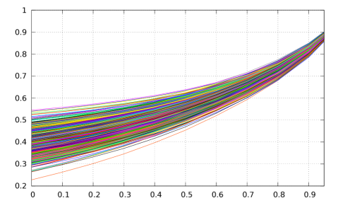
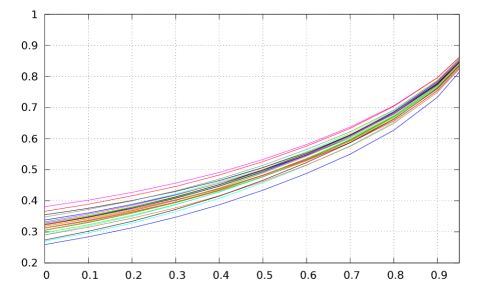
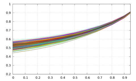
Figure 10: Distances between all pairs of genuine papers (top), all pairs of fake papers (middle), and between genuine and fake papers (bottom) in Experiment 1, depending on the discounting factor. Lines between points have been added for visualization.

Finally, we show in Table 3 (see also Fig. 10 in the appendix for a visualization) how the mutual distances between the 50 papers evolve depending on the discounting factor. One can see that at $\lambda=0$, the three types of mutual distances are overlapping, whereas at $\lambda=.95$, they are almost separated into three bands: .81-.86 for fake papers, .86-.90 for genuine papers, and .89-.92 for comparing genuine with fake papers.

Altogether, we conclude from the first experiment that our inter-textual distance can achieve a safe separation between genuine and fake papers in our corpus, and that the separation is stronger for higher discounting factors.

4.3 Second experiment

The second experiment was conducted on 97 papers from arxiv.org, 50 fake papers generated by a modified SCIgen program, and 50 fake papers generated by automogensen. The arxiv papers were between 1400 and 15,000 words long, the SCIgen papers between 2700 and 12,000 words, and the automogensen papers between 4,000 and 10,000 words. The distances were computed for discounting factors $0$, $.4$, $.8$ and $.95$; with our software, computations took about four hours for each discounting factor.

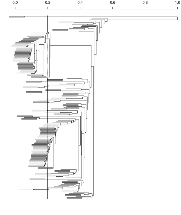
Figure 11: Dendrogram for Experiment 2, using average clustering, for discounting factor $0$. Black dots mark arxiv papers, green marks SCIgen papers, and automogensen papers are marked red.

We show the dendrograms using average clustering in Figs. 11 to 14 in the appendix; they appear somewhat inconclusive. One clearly notices the SCIgen and automogensen parts of the corpus, but the arxiv papers have wildly varying distances and disturb the dendrogram. One interesting observation is that with discounting factor $0$, the automogensen papers have small mutual distances compared to the arxiv corpus, comparable to the SCIgen papers’ mutual distances, whereas with high discounting ($.95$), the automogensen papers’ mutual distances look more like the arxiv papers’. Note that the difficulties in clustering appear also with discounting factor $0$, hence also when only matching words.

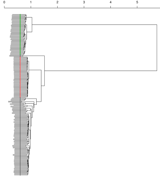
Figure 3: Dendrogram for Experiment 2, using Ward clustering, for discounting factor $.95$. Black dots mark arxiv papers, green marks SCIgen papers, and automogensen papers are marked red.

The dendrograms using Ward clustering, however, do show a clear distinction between the three types of papers. We can only show one of them here, for $\lambda=.95$ in Fig. 3; the rest are available in appendix. One clearly sees the SCIgen cluster (top) separated from all other papers, and then the automogensen cluster (middle) separated from the arxiv cluster.

There is, though, one anomaly: two arxiv papers have been “wrongly” grouped into their own cluster (between the SCIgen and the automogensen clusters). Looking at these papers, we noticed that here our pdf-to-text conversion had gone wrong: the papers’ text was all garbled, consisting only of “AOUOO OO AOO EU OO OU AO” etc. The dendrograms rightly identify these two papers in their own cluster; in the dendrograms using average clustering, this garbled cluster consistently has distance $1$ to the other clusters.

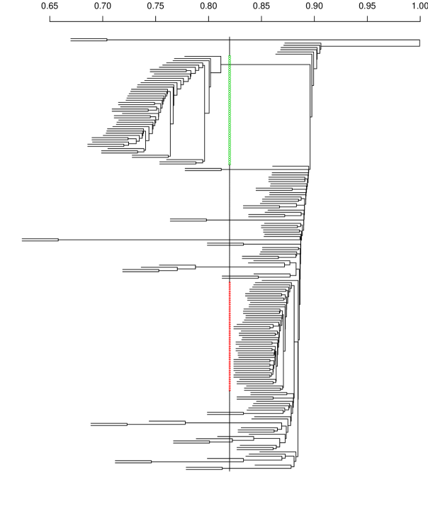
Figure 14: Dendrogram for Experiment 2, using average clustering, for discounting factor $.95$. Black dots mark arxiv papers, green marks SCIgen papers, and automogensen papers are marked red.

We also notice in the dendrogram with average clustering and discounting factor $.95$ (Fig. 14 in the appendix) that some of the arxiv papers with small mutual distances have the same authors and are within the same subject. This applies to [26] vs. [27] and to [31] vs. [32]. These similarities appear much more clearly in the $\lambda=.95$ dendrogram than in the ones with lower discounting factor.

As a conclusion from this experiment, we can say that whereas average clustering had some difficulties in distinguishing between fake and arxiv papers, Ward clustering did not have any problems. The only effect of the discounting factor we could see was in identifying similar arxiv papers. We believe that one reason for the inconclusiveness of the dendrograms with average clustering is the huge variety of the arxiv corpus. Whereas the genuine corpus of the first experiment included only papers from the verification sub-field of theoretical computer science, the arxiv corpus is comprised of papers from a diverse selection of research areas within computer science, including robotics, network detection, computational geometry, constraint programming, numerical simulation and many others. Hence, the intra-corpus variation in the arxiv corpus hides the inter-corpus variations.

5 Conclusion and Further Work

We believe we have collected enough evidence that our global inter-textual distance provides an interesting alternative, or supplement, to the standard 1-gram distance. In our experiments, we have seen that measuring inter-textual distance with high discounting factor enables us to better differentiate between similar and dissimilar texts. More experiments will be needed to identify areas where our global matching provides advantages over pure 1-gram matching.

With regard to identifying fake scientific papers, we remark that, according to [16], “[u]sing [the 1-gram distance] to detect SCIgen papers relies on the fact that […] the SCIgen vocabulary remains quite poor”. Springer has recently announced [29] that they will integrate “[a]n automatic SCIgen detection system […] in [their] submission check system”, but they also notice that the “intention [of fake papers’ authors] seems to have been to increase their publication numbers and […] their standing in their respective disciplines and at their institutions”; of course, auto-detecting SCIgen papers does not change these motivations. It is thus reasonable to expect that generators of fake papers will get better, so that also better tools will be needed to detect them. We propose that our phrase-based distance may be such a tool.

There is room for much improvement in our distance definition. For once, we perform no tagging of words which could identify different spellings or inflections of the same word. This could easily be achieved by, using for example the Wordnet database, replacing our binary distance between words in Eq. (1) with a quantitative measure of word similarity. For the second, we take no consideration of omitted words in a phrase; our position match calculation in Eq. (2) cannot see when two phrases become one-off like in “the quick brown fox jumps…” vs. “the brown fox jumps…”.

Our inter-textual distance is inspired by our work in [6, 5, 7] and other papers, where we define distances between arbitrary transition systems. Now a text is a very simple transition system, but so is a text with “one-off jumps” like the one above. Similarly, we can incorporate swapping of words into our distance, so that we would be computing a kind of discounted Damerau-Levenshtein distance [4] (related approaches, generally without discounting, are used for sequence alignment in bioinformatics [20, 28]). We have integrated this approach in an experimental version of our textdist tool.

Appendix

Proof of Theorem 2.1

Let $\phi$ be an optimal matching in $D_{\textup{pm}}$ and let $d_{\textup{pm}}(i,\phi(i),0)=1$ (if such $i$ does not exist, then $d_{2}(A,B,0)=0$ and we are done). Let $w=a_{i}$. Assume that there is $b_{j}=w$ for which $d_{\textup{pm}}(\phi^{-1}(j),j)=1$, then we can define a new permutation $\phi^{\prime}$ by $\phi^{\prime}(i)=j$ and $\phi^{\prime}(\phi^{-1}(j))=\phi(i)$ (and otherwise, values like $\phi$), and $\phi^{\prime}$ is a better matching than $\phi$, a contradiction.

Hence $d_{\textup{pm}}(\phi^{-1}(j),j)=0$ for all $j$ such that $b_{j}=w$. In other words, $d_{\textup{pm}}(i,\phi(i),0)=1$ marks the fact that the word $w=a_{i}$ occurs one time more in $A$ than in $B$. The same holds for all other indices $i$ for which $w=a_{i}$ and $d_{\textup{pm}}(i,\phi(i),0)=1$, so that

$$|F_{A}(w)-F_{B}(w)|=|\{i\mid a_{i}=w,d_{\textup{pm}}(i,\phi(i),0)=1\}|$$

in this case.

Similarly, if we let $v=b_{\phi(i)}$, then $d_{\textup{pm}}(i,\phi(i),0)=1$ marks the fact that the word $v$ occurs one time more in $B$ than in $A$. Collecting these two, we see that

$$|F_{A}(w)-F_{B}(w)|=|\{i\mid a_{i}=w,d_{\textup{pm}}(i,\phi(i),0)=1\}|\\ +|\{j\mid b_{j}=w,d_{\textup{pm}}(\phi^{-1}(j),j,0)=1\}|$$

for all words $w\in A\circ B$. Thus

$$\sum_{w\in A\circ B}|F_{A}(w)-F_{B}(w)| =\sum_{w\in A\circ B}|\{i\mid a_{i}=w,d_{\textup{pm}}(i,\phi(i),0)=1\}|$$

$$\qquad+\sum_{w\in A\circ B}|\{j\mid b_{j}=w,d_{\textup{pm}}(\phi^{-1}(j),j,0)=1\}|$$

$$=|\{i\mid d_{\textup{pm}}(i,\phi(i),0)=1\}|$$

$$\qquad+|\{j\mid d_{\textup{pm}}(\phi^{-1}(j),j,0)=1\}|$$

$$=\sum_{i}d_{\textup{pm}}(i,\phi(i),0)+\sum_{j}d_{\textup{pm}}(\phi^{-1}(j),j,0)$$

$$=2\sum_{i}d_{\textup{pm}}(i,\phi(i),0)\,,$$

so that

$$d_{1}(A,B) =\frac{\sum_{w\in A\circ B}|F_{A}(w)-F_{B}(w)|}{2N_{A}}$$

$$=\frac{\sum_{i}d_{\textup{pm}}(i,\phi(i),0)}{N_{A}}=d_{2}(A,B,0)\,,$$

because $\phi$ was assumed optimal.

Figure 4: Dendrograms for Experiment 1, using average clustering, for discounting factors $0$ (top left), $.1$ (top right), $.2$ (bottom left) and $.3$ (bottom right), respectively. Fake papers are numbered 28-31 (Antkare) and 43-46 (SCIgen), the others are genuine.

Figure 5: Dendrograms for Experiment 1, using average clustering, for discounting factors $.4$ (top left), $.5$ (top right), $.6$ (bottom left) and $.7$ (bottom right), respectively. Fake papers are numbered 28-31 (Antkare) and 43-46 (SCIgen), the others are genuine.

Figure 6: Dendrograms for Experiment 1, using average clustering, for discounting factors $.8$ (top left), $.9$ (top right) and $.95$ (bottom), respectively. Fake papers are numbered 28-31 (Antkare) and 43-46 (SCIgen), the others are genuine.

Figure 7: Dendrograms for Experiment 1, using Ward clustering, for discounting factors $0$ (top left), $.1$ (top right), $.2$ (bottom left) and $.3$ (bottom right), respectively. Fake papers are numbered 28-31 (Antkare) and 43-46 (SCIgen), the others are genuine.

Figure 8: Dendrograms for Experiment 1, using Ward clustering, for discounting factors $.4$ (top left), $.5$ (top right), $.6$ (bottom left) and $.7$ (bottom right), respectively. Fake papers are numbered 28-31 (Antkare) and 43-46 (SCIgen), the others are genuine.

Figure 9: Dendrograms for Experiment 1, using Ward clustering, for discounting factors $.8$ (top left), $.9$ (top right) and $.95$ (bottom), respectively. Fake papers are numbered 28-31 (Antkare) and 43-46 (SCIgen), the others are genuine.

Figure 12: Dendrogram for Experiment 2, using average clustering, for discounting factor $.4$. Black dots mark arxiv papers, green marks SCIgen papers, and automogensen papers are marked red.

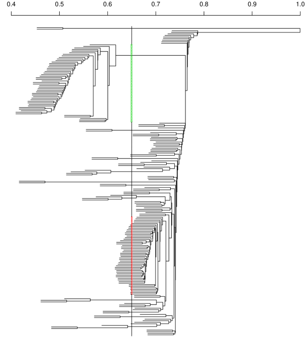
Figure 13: Dendrogram for Experiment 2, using average clustering, for discounting factor $.8$. Black dots mark arxiv papers, green marks SCIgen papers, and automogensen papers are marked red.

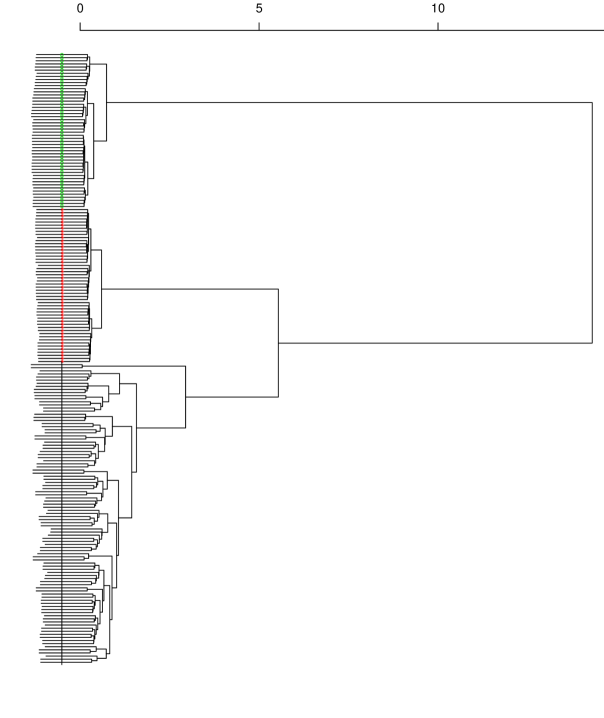
Figure 15: Dendrogram for Experiment 2, using Ward clustering, for discounting factor $0$. Black dots mark arxiv papers, green marks SCIgen papers, and automogensen papers are marked red.

Figure 16: Dendrogram for Experiment 2, using Ward clustering, for discounting factor $.4$. Black dots mark arxiv papers, green marks SCIgen papers, and automogensen papers are marked red.

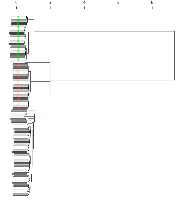
Figure 17: Dendrogram for Experiment 2, using Ward clustering, for discounting factor $.8$. Black dots mark arxiv papers, green marks SCIgen papers, and automogensen papers are marked red.

References

- [1] E. Asarin and A. Degorre. Volume and entropy of regular timed languages. hal, 2009. http://hal.archives-ouvertes.fr/hal-00369812.
- [2] N. Basset and E. Asarin. Thin and thick timed regular languages. In [8].
- [3] M. A. Cortelazzo, P. Nadalutti, and A. Tuzzi. Improving Labbé’s intertextual distance: Testing a revised version on a large corpus of italian literature. J. Quant. Linguistics, 20(2):125–152, 2013.
- [4] F. Damerau. A technique for computer detection and correction of spelling errors. Commun. ACM, 7(3):171–176, 1964.
- [5] U. Fahrenberg and A. Legay. Generalized quantitative analysis of metric transition systems. In APLAS, vol. 8301 of Lect. Notes Comput. Sci. Springer, 2013.
- [6] U. Fahrenberg and A. Legay. The quantitative linear-time–branching-time spectrum. Theor. Comput. Sci., 2013. Online first. http://dx.doi.org/10.1016/j.tcs.2013.07.030.
- [7] U. Fahrenberg, A. Legay, and C. R. Thrane. The quantitative linear-time–branching-time spectrum. In FSTTCS, vol. 13 of LIPIcs, 2011.
- [8] U. Fahrenberg and S. Tripakis, eds. Formal Modeling and Analysis of Timed Systems - 9th Int. Conf., vol. 6919 of Lect. Notes Comput. Sci. Springer, 2011.
- [9] B. R. Haverkort. Formal modeling and analysis of timed systems: Technology push or market pull? In [8].
- [10] L. Kaufman and P. J. Rousseeuw. Finding Groups in Data: An Introduction to Cluster Analysis. Wiley Interscience. Wiley, 1990.
- [11] S. A. Kharmeh, K. Eder, and D. May. A design-for-verification framework for a configurable performance-critical communication interface. In [8].
- [12] H. W. Kuhn. The Hungarian method for the assignment problem. Naval Research Logistics Quarterly, 2(1-2):83–97, 1955.
- [13] C. Labbé. Ike Antkare, one of the great stars in the scientific firmament. ISSI Newsletter, 6(2):48–52, 2010. http://hal.archives-ouvertes.fr/hal-00713564.
- [14] C. Labbé and D. Labbé. Inter-textual distance and authorship attribution. Corneille and Molière. J. Quant. Linguistics, 8(3):213–231, 2001.
- [15] C. Labbé and D. Labbé. A tool for literary studies: Intertextual distance and tree classification. Literary Linguistic Comp., 21(3):311–326, 2006.
- [16] C. Labbé and D. Labbé. Duplicate and fake publications in the scientific literature: how many SCIgen papers in computer science? Scientometrics, 94(1):379–396, 2013.
- [17] D. Labbé. Experiments on authorship attribution by intertextual distance in English. J. Quant. Linguistics, 14(1):33–80, 2007.
- [18] C.-Y. Lin and E. H. Hovy. Automatic evaluation of summaries using n-gram co-occurrence statistics. In HLT-NAACL, 2003.
- [19] C.-Y. Lin and F. J. Och. Automatic evaluation of machine translation quality using longest common subsequence and skip-bigram statistics. In ACL. ACL, 2004.
- [20] S. B. Needleman and C. D. Wunsch. A general method applicable to the search for similarities in the amino acid sequence of two proteins. J. Molecular Bio., 48(3):443–453, 1970.
- [21] R. V. Noorden. Publishers withdraw more than 120 gibberish papers. Nature News & Comment, Feb. 2014. http://dx.doi.org/10.1038/nature.2014.14763.
- [22] K. Papineni, S. Roukos, T. Ward, and W.-J. Zhu. BLEU: a method for automatic evaluation of machine translation. In ACL. ACL, 2002.
- [23] S. Sankaranarayanan, H. Homaei, and C. Lewis. Model-based dependability analysis of programmable drug infusion pumps. In [8].
- [24] J. Savoy. Authorship attribution: A comparative study of three text corpora and three languages. J. Quant. Linguistics, 19(2):132–161, 2012.
- [25] J. Savoy. Authorship attribution based on specific vocabulary. ACM Trans. Inf. Syst., 30(2):12, 2012.
- [26] S. T. Smith, E. K. Kao, K. D. Senne, G. Bernstein, and S. Philips. Bayesian discovery of threat networks. CoRR, abs/1311.5552v1, 2013.
- [27] S. T. Smith, K. D. Senne, S. Philips, E. K. Kao, and G. Bernstein. Network detection theory and performance. CoRR, abs/1303.5613v1, 2013.
- [28] T. Smith and M. Waterman. Identification of common molecular subsequences. J. Molecular Bio., 147(1):195–197, 1981.
- [29] Springer second update on SCIgen-generated papers in conference proceedings. Springer Statement, Apr. 2014. http://www.springer.com/about+springer/media/statements?SGWID=0-1760813-6-1460747-0.
- [30] F. Tomasi, I. Bartolini, F. Condello, M. Degli Esposti, V. Garulli, and M. Viale. Towards a taxonomy of suspected forgery in authorship attribution field. A case: Montale’s Diario Postumo. In DH-CASE. ACM, 2013.
- [31] A. Ulusoy, S. L. Smith, X. C. Ding, and C. Belta. Robust multi-robot optimal path planning with temporal logic constraints. CoRR, abs/1202.1307v2, 2012.
- [32] A. Ulusoy, S. L. Smith, X. C. Ding, C. Belta, and D. Rus. Optimal multi-robot path planning with temporal logic constraints. CoRR, abs/1107.0062v1, 2011.