A dictionary between $\mathrm{R}$-operators, on-shell graphs and Yangian algebras

1 Introduction and outline

$\mathcal{N}=4$ super-Yang–Mills (sYM) theory is the maximally supersymmetric four-dimensional gauge theory not including gravity [1, 2]. It is a gauge theory with gauge group $\mathrm{SU}(N_{c})$; the spectrum includes a single $\mathcal{N}=4$ massless multiplet, consisting of one gauge field, four Weyl fermions and six real scalars, all transforming in the adjoint representation of the gauge group. One of the most remarkable properties of this theory is that it is superconformally invariant even at the quantum level [3, 4, 5, 6] – its symmetry group effectively being $\mathrm{PSU}(2,2|4)$.

In recent years, the study of scattering amplitudes in $\mathcal{N}=4$ sYM theory unveiled a rich underlying structure. One of the most striking discoveries is the hidden dual superconformal symmetry of tree-level amplitudes [7]; the closure of the ordinary superconformal algebra and this dual superconformal symmetry is the Yangian algebra $\mathrm{Y}[\mathfrak{psu}(2,2|4)]$ [8]. Although the tree-level S-matrix enjoys this symmetry, Yangian invariance is broken at loop level due to IR divergences.

An important tool to investigate the rich structure arising from amplitudes in $\mathcal{N}=4$ sYM theory is the so-called Grassmannian formalism [9, 10, 11, 12, 13]. While the original formulation allowed to express leading singularities of amplitudes in terms of contour integrals over a suitable Grassmannian manifold, it was subsequently shown that it is possible to identify the correct contours leading to the Britto–Cachazo–Feng–Witten (BCFW) decomposition of tree- and loop-level amplitudes. The approach was later generalised to the study of on-shell graphs (or diagrams) [14], planar bicolored graphs that correspond to Yangian invariants. These diagrams were studied and generalised in refs. [15, 16] (see also [17]), where it was shown that it is possible to deform the external helicities to complex values while preserving Yangian invariance.

Recently, a new method for the study of Yangian invariants related to scattering amplitudes was proposed in refs. [18, 19]. The authors employ an algebraic approach to construct Yangian invariants by defining a set of operators acting on a suitable vacuum. Their construction is manifestly Yangian invariant at each step and is shown to yield the correct form of (deformed) tree-level MHV scattering amplitudes. The authors argue that the same approach can be used to construct all tree-level amplitudes in a manifestly Yangian-invariant way by building single channels via the inverse-soft-limit construction [20]. A similar construction arose in the context of the Bethe-ansatz approach in ref. [21].

The aim of this paper is to study the algebraic approach for the construction of Yangian invariants and tree-level scattering amplitudes and relate it to the known formulations of Yangian invariants in $\mathcal{N}=4$ sYM theory. In sec. 2 we review some of the properties of scattering amplitudes in $\mathcal{N}=4$ sYM theory, focusing mainly on the symmetries of the tree-level S-matrix. An important part of the review concerns the Grassmannian formalism for scattering amplitudes [9, 10, 11, 12, 13] in terms of on-shell diagrams [14]. One of the most important results for the current article is the correspondence between the Yangian-invariant leading singularities of amplitudes and decorated permutations. We will see that a similar combinatorial construction arises also in the language of refs. [18, 19].

In sec. 3 we discuss the algebraic framework underlying the construction of refs. [18, 19]. In these papers the authors show how to construct invariants under the Yangian of $\mathfrak{gl}(4|4)$ via some suitable operators. These operators (called $\mathrm{R}$-operators) act on generalised functions defined on on-shell superspace as

$$\mathrm{R}_{ab}(u)f(\lambda_{a},\tilde{\lambda}_{a},\tilde{\eta}_{a},\lambda_{b},\tilde{\lambda}_{b},\tilde{\eta}_{b}):=\int\frac{\mathrm{d}z}{z^{1+u}}f(\lambda_{a}-z\lambda_{b},\tilde{\lambda}_{a},\tilde{\eta}_{a},\lambda_{b},\tilde{\lambda}_{b}+z\tilde{\lambda}_{a},\tilde{\eta}_{b}+z\tilde{\eta}_{a})\ .$$ (1.1)

The “vacuum state” used as starting point of the construction is a combination of superconformally invariant delta functions. The operator $\mathrm{R}_{ab}$ is introduced as an intertwiner of representations of the Yangian algebra. It is evident that its action has a clear “physical” interpretation: it performs a BCFW shift. A function defined in this way on on-shell superspace is a Yangian invariant if it is an eigenfunction of the monodromy matrix naturally arising in this context.

We compute and analyse in detail the low-multiplicity Yangian invariants arising from this construction. We show that it is possible to construct the single channels of the BCFW decomposition of the six-point NMHV amplitude starting from a single invariant, which we will subsequently show to be equivalent to the top-cell on-shell diagram of ref. [14]. Analysing the symmetries of the Yangian invariants in detail allows us to associate a permutation to each of them in a natural way.

Section 4 relates the algebraic construction of Yangian invariants with the on-shell diagram formalism. We will show that the three ways of encoding a Yangian invariant discussed – $\mathrm{R}$-operator approach, associated permutation, on-shell diagrams – can be actually translated one into the other.

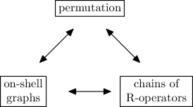
Figure 1: Three equivalent ways of describing Yangian invariants.

After showing how to associate an on-shell diagram to a Yangian-invariant chain of $\mathrm{R}$-operators, we demonstrate how to associate a Yangian-invariant $\mathrm{R}$-chain to a permutation and vice versa, thus completing the three-way correspondence. Parity and dihedral symmetries can be nicely interpreted in terms of permutations. The section is concluded with the discussion of the six- and seven-point NMHV Yangian invariants. Finally, we summarise the results and consider some possible future directions of inquiry in the concluding section.

Note: In the process of preparing this article for publication, we learnt about the paper [22], which shares some conclusions with our present project. We thank the authors for providing us with a draft of their paper.

2 Superamplitudes in $\mathcal{N}=4$ super-Yang–Mills theory

In this section we will review the main features of scattering amplitudes in $\mathcal{N}=4$ sYM theory and some of the tools available to compute them. We will focus on some more recent developments in the study of the underlying symmetries of the (planar) S-matrix.

For the study of scattering amplitudes in $\mathcal{N}=4$ sYM it is convenient to introduce the so-called on-shell superspace variables $(\lambda^{\alpha},\tilde{\lambda}_{\dot{\alpha}},\tilde{\eta}^{A})$ [23], which are the supersymmetric extension of the ordinary spinor-helicity variables. Here, Greek and upper case Latin indices are indices of the fundamental representation of $\mathrm{SL}(2)$ and $\mathrm{SU}(4)$, respectively.

Since the $\mathcal{N}=4$ multiplet is CPT self-conjugate, it can be expressed as a single superfield defined on the on-shell superspace

$$\Phi(\lambda,\tilde{\lambda},\tilde{\eta}):=g^{+}+\tilde{\eta}^{A}\psi_{A}+\,\frac{1}{2}\tilde{\eta}^{A}\tilde{\eta}^{B}\,\phi_{AB}+\frac{1}{3!}\epsilon_{ABCD}\,\tilde{\eta}^{A}\tilde{\eta}^{B}\tilde{\eta}^{C}\,\bar{\psi}^{D}+\frac{1}{4!}\epsilon_{ABCD}\,\tilde{\eta}^{A}\tilde{\eta}^{B}\tilde{\eta}^{C}\tilde{\eta}^{D}\,g^{-}\ .$$ (2.1)

The colour-ordered tree-level scattering amplitudes of the full supermultiplet can be expressed as functions on $n$ copies of the on-shell superspace as

$$\mathcal{A}(\Phi_{1},\dots,\Phi_{n}):=\mathcal{A}_{n;2}\,\mathcal{P}_{n}\ ,$$ (2.2)

where

$$\mathcal{A}_{n;2}=\frac{\delta^{4}\bigl{(}\sum_{i=1}^{n}\lambda_{i}\tilde{\lambda}_{i}\bigr{)}\delta^{0|8}\bigl{(}\sum_{i=1}^{n}\lambda_{i}\tilde{\eta}_{i}\bigr{)}}{\langle 12\rangle\langle 23\rangle\dots\langle n1\rangle}$$ (2.3)

is the supersymmetric version of the MHV gluon scattering amplitude [23], and our conventions for spinor brackets are

$$\langle ij\rangle =\lambda_{i}^{\alpha}\lambda_{j\alpha}\ , \qquad[ij] =\tilde{\lambda}_{i\dot{\alpha}}\tilde{\lambda}_{j}^{\dot{\alpha}}\ ,$$

$$\lambda_{\alpha}=\epsilon_{\alpha\beta}\lambda^{\beta}\ ,\qquad\lambda^{\beta} =\epsilon^{\beta\gamma}\lambda_{\gamma}\ , \qquad\tilde{\lambda}_{\dot{\alpha}} =\epsilon_{\dot{\alpha}\dot{\beta}}\tilde{\lambda}^{\dot{\beta}}\ ,\qquad\tilde{\lambda}^{\dot{\beta}}=\epsilon^{\dot{\beta}\dot{\gamma}}\tilde{\lambda}_{\dot{\gamma}}$$

with $\epsilon_{12}=\epsilon_{\dot{1}\dot{2}}=-1$.

The function $\mathcal{P}_{n}$ is the sum

$$\mathcal{P}_{n}=\mathcal{P}_{n;0}+\mathcal{P}_{n;1}+\dots+\mathcal{P}_{n;n-4}\ ,$$ (2.4)

where each ${\cal P}_{n;k-2}$ is a function of homogeneous Grassmann degree $4(k-2)$. The quantity $k-2$ determines the $\mathrm{MHV}$ level of the amplitude. The $n$-point $\mathrm{N}^{k-2}\mathrm{MHV}$ amplitude is the term $\mathcal{A}_{n;k}:=\mathcal{A}_{n;2}\mathcal{P}_{n;k-2}$; obviously, $\mathcal{P}_{n;0}=1$.

2.1 Symmetries of tree-level scattering amplitudes

Scattering amplitudes in $\mathcal{N}=4$ sYM are invariant under the action of the generators of $\mathfrak{psu}(2,2|4)$ (the representation of these generators on the space of functions on on-shell superspace was derived in ref. [24]). The additional requirement of physicality external legs amounts to imposing the invariance of the amplitude under the action of the central charge

$$C_{i}=\lambda_{i}^{\alpha}\frac{\partial}{\partial\lambda_{i}^{\alpha}}-\tilde{\lambda}_{i}^{\dot{\alpha}}\frac{\partial}{\partial\tilde{\lambda}_{i}^{\dot{\alpha}}}-\tilde{\eta}_{i}^{A}\frac{\partial}{\partial\tilde{\eta}_{i}^{A}}+2\ ,$$ (2.5)

where the index $i=1,\dots,n$ labels the external legs. We will henceforth consider invariance under the centrally extended algebra $\mathfrak{su}(2,2|4)$.

A striking property of tree-level amplitudes in $\mathcal{N}=4$ sYM is that, in addition to the ordinary invariance under $\mathrm{PSU}(2,2|4)$, they are covariant under a dual superconformal symmetry, acting on the coordinates of the dual space [7]. In ref. [8] it was shown that the closure of the realisations of these two copies of $\mathfrak{psu}(2,2|4)$ is the Yangian algebra $\mathrm{Y}[\mathfrak{psu}(2,2|4)]$.

An $n$-point tree-level scattering amplitude can be expressed as a sum of Yangian invariants. A suitable way to compute such a decomposition is provided by the supersymmetric version of the Britto–Cachazo–Feng–Witten (BCFW) recursion relations [25, 26, 10, 27]. These relations express a tree-level amplitude as a sum of terms constructed out of lower-multiplicity on-shell amplitudes. In these terms, the $n$-point $\mathrm{N}^{k-2}\mathrm{MHV}$ superamplitude reads

$$\mathcal{A}_{n;k}(1,\dots,n)=\sum_{\begin{subarray}{c}n_{L}+n_{R}=n+2\\ k_{L}+k_{R}=k+1\end{subarray}}\int\mathrm{d}^{4}P\,\mathrm{d}^{4}\tilde{\eta}\;\mathcal{A}_{L}\Bigl{(}\{p_{1},\hat{\tilde{\eta}}_{1}\},\dots,\{p_{n_{L}-1},\tilde{\eta}_{n_{L}-1}\},\{p,\tilde{\eta}\}\Bigr{)}\times$$ (2.6)

$$\times\frac{1}{P^{2}}\mathcal{A}_{R}\Bigl{(}\{-p,\tilde{\eta}\},\{p_{n_{R}+1},\tilde{\eta}_{n_{R}+1}\},\dots,\{p_{n},\hat{\tilde{\eta}}_{n}\}\Bigr{)}\ ,$$

where the superamplitudes $\mathcal{A}_{L,R}$ include the delta functions, $p=P+z_{P_{L}}\lambda_{1}\tilde{\lambda}_{n}$ and $z_{P_{L}}=P_{L}^{2}/\langle 1|P_{L}|n]$. In this sum each term is Yangian invariant.

$\;=\;$ $\;+\;$ $\;+\;$

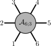
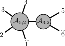
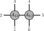
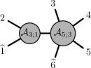
Figure 2: BCFW decomposition of the six-point NMHV amplitude.

2.2 On-shell graphs and permutations

In ref. [14] the authors introduced the formalism of so-called on-shell diagrams (or on-shell graphs) to analyse the properties of Yangian invariants and scattering amplitudes in $\mathcal{N}=4$ sYM . These diagrams are constructed by gluing two basic trivalent vertices – “black” and “white” vertices, which correspond to the three-point $\mathrm{MHV}$ and $\overline{\mathrm{MHV}}$ amplitudes, respectively.

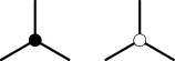
Figure 3: Trivalent building blocks for on-shell graphs.

The authors show that these diagrams correspond to Yangian invariants; this correspondence is encoded in the map from on-shell graphs to integrals over a suitable Grassmannian manifold $G(k,n)$. This formalism is an extension of the Grassmannian formulation for scattering amplitudes previously developed in refs. [9, 12, 11, 13]. The pair $(k,n)$ consists of the $\mathrm{MHV}$ level $k$ and the multiplicity $n$ of the amplitude the on-shell graph is related to; they are linked to $n_{\text{w}},\,n_{\text{b}},\,n_{\text{i}}$ (the number of white vertices, black vertices and internal lines of the graph, respectively) via

$$n=3(n_{\text{w}}+n_{\text{b}})-2n_{\text{i}}\ ,\qquad k=n_{\text{w}}+2n_{\text{b}}-n_{\text{i}}\ .$$ (2.7)

One of the most important results in [14] is the construction of a map between a subset of on-shell graphs (so-called reduced, related to tree-level amplitudes) and decorated permutations. A decorated permutation is an injective map

$$\sigma\;:\;\{1,\dots,n\}\;\;\to\;\;\{1,\dots,2n\}$$ (2.8)

such that $i\leq\sigma(i)\leq i+n$ and $\sigma\;\mathrm{mod}\,n$ is an ordinary permutation. The map is constructed starting from the on-shell graph as follows: starting from the $i$-th leg, one follows the internal lines turning right at each black vertex and left at each white vertex; the external leg $j$ this path ends on yields $\sigma(i)$, with the identification

$$\sigma(i)=j\quad\text{if}\;j>i,\qquad\sigma(i)=j+n\quad\text{if}\;j<i\ .$$ (2.9)

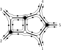
,          $\begin{pmatrix}1&2&3&4&5\\ \downarrow&\downarrow&\downarrow&\downarrow&\downarrow\\ 3&4&5&6&7\end{pmatrix}$

Figure 4: Double-line notation and decorated permutation for the five-point MHV on-shell diagram.

There are different on-shell graphs that correspond to the same decorated permutation; however, all the on-shell graphs that correspond to a given permutation can be mapped one into the other via two actions: merger and square move, depicted in fig. 5.

$\;\equiv\;$ ,                  $\;\equiv\;$ .

Figure 5: Square move and merger.

All diagrams that can be related via these two transformations are associated to the same Yangian invariant. The authors of [14] therefore conclude that there is a one-to-one map between Yangian invariants (appearing in the tree-level amplitudes of $\mathcal{N}=4$ sYM ) and decorated permutations or that, equivalently, the invariant information of a (reduced) on-shell graph is encoded in the associated permutation.

It is possible to derive the BCFW recursion relation in terms of on-shell graphs. For a $(k,n)$ tree-level amplitude $\mathcal{A}_{n;k}$ (or $\mathcal{A}_{n}^{(k)}$), all BCFW channels can be obtained starting from a single on-shell graph (the top-cell graph) corresponding to a permutation which is a cyclic shift by $k$.

This fact allows to construct a representative on-shell graph for the top-cell easily (as first shown in ref. [28] and reviewed in ref. [15]). It is done as follows: for the top-cell graph of a $(k,n)$ amplitude (corresponding to the top-cell of the positive Grassmannian $G_{+}(k,n)$) draw $k$ horizontal lines, $(n-k)$ vertical lines so that the leftmost and topmost are boundaries, then substitute the three-crossings and four-crossings as in fig. 6.

$$\begin{array}[]{ccc}\parbox[c]{13.0086pt}{\leavevmode\hbox{\includegraphics{Fig_plabicwv1.mps}}}&\;\Leftrightarrow&\parbox[c]{13.0086pt}{\leavevmode\hbox{\includegraphics{Fig_plabicwv2.mps}}}\\ &&\\ \parbox[c]{6.5043pt}{\leavevmode\hbox{\includegraphics{Fig_plabicbv1.mps}}}&\;\Leftrightarrow&\parbox[c]{7.9497pt}{\leavevmode\hbox{\includegraphics{Fig_plabicbv2.mps}}}\\ &&\\ \parbox[c]{13.0086pt}{\leavevmode\hbox{\includegraphics{Fig_plabicdv1.mps}}}&\;\Leftrightarrow&\parbox[c]{15.1767pt}{\leavevmode\hbox{\includegraphics{Fig_plabicdv2.mps}}}\end{array}$$

Figure 6: Construction of a representative on-shell graph for the top-cell of a $(k,n)$ amplitude.

The on-shell graphs corresponding to the BCFW channels are then obtained by removing $(k-2)(n-k-2)$ edges from the top-cell graph. Note that not all edges are removable, and the removable ones can be identified with a purely combinatorial procedure. The removal of an edge can be interpreted in terms of the Grassmannian integral as the residue around a singularity of the integrand.

The choice of which on-shell graphs obtained this way correspond to a BCFW decomposition of the amplitude relies on the imposition of the correct unitarity constraint and collinear limits; one of the recursive diagrammatic solution to the BFCW recursion relations in terms of on-shell graphs is depicted in fig. 7.

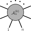
$\;=\;$ $\displaystyle\;+\;\sum_{\begin{subarray}{c}k_{L}+k_{R}=k+1\\ n_{L}+n_{R}=n+2\end{subarray}}$ $\;+\;$

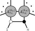
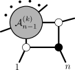
Figure 7: Diagrammatic solution to the BCFW recursion relations in terms of on-shell graphs.

From the above discussion, we can infer that for MHV amplitudes there is one single on-shell graph that corresponds to the amplitude – the top-cell graph – and the corresponding permutation is just a cyclic shift by two. The first nontrivial example of a BCFW decomposition is the six-point NMHV amplitude, which is obtained as a sum of three on-shell graphs corresponding to the permutations reported in fig. 8.

$$\begin{array}[]{cccc}\parbox[c]{52.7571pt}{\leavevmode\hbox{\includegraphics{Fig6pts_gen.mps}}}$\;=$&\parbox[c]{61.4295pt}{\leavevmode\hbox{\includegraphics{Fig_6pt2.mps}}}$\;+$&\parbox[c]{67.2111pt}{\leavevmode\hbox{\includegraphics{Fig_6pt1.mps}}}$\;+$&\parbox[c]{61.4295pt}{\leavevmode\hbox{\includegraphics{Fig_6pt3.mps}}}\\ &&&\\ &\Big{(}\begin{smallmatrix}1&2&3&4&5&6\\ \downarrow&\downarrow&\downarrow&\downarrow&\downarrow&\downarrow\\ 4&5&6&7&9&8\end{smallmatrix}\Big{)}&\Big{(}\begin{smallmatrix}1&2&3&4&5&6\\ \downarrow&\downarrow&\downarrow&\downarrow&\downarrow&\downarrow\\ 3&5&6&7&8&10\end{smallmatrix}\Big{)}&\Big{(}\begin{smallmatrix}1&2&3&4&5&6\\ \downarrow&\downarrow&\downarrow&\downarrow&\downarrow&\downarrow\\ 5&4&6&7&8&9\end{smallmatrix}\Big{)}\,.\end{array}$$

Figure 8: BCFW decomposition of the six-point NMHV amplitude, with the decorated permutations corresponding to the on-shell graphs.

2.3 Deformed on-shell graphs and Yangian invariants

In refs. [15, 16], the authors studied a generalisation of on-shell graphs (and related Yangian invariants). This generalisation relaxes the condition of physicality of the external legs of the on-shell graph. Stated explicitly, the deformed $n$-point Yangian invariant $\mathcal{Y}$ associated with a given on-shell graph will satisfy

$$\mathfrak{C}_{i}\cdot\mathcal{Y}(1,\dots,n)=c_{i}\,\mathcal{Y}(1,\dots,n)$$ (2.10)

with $c_{i}\neq 0$, in general. A deformed on-shell graph can be built by gluing together two trivalent building blocks, that correspond just to the deformation of the three-point $\mathrm{MHV}$ and $\overline{\mathrm{MHV}}$ amplitudes. As this deformation is switched on, one must pay attention to what happens to the Yangian generators: in fact the representation that annihilates this deformed objects is the evaluation representation with evaluation parameters $u_{i}$ different at each site. The level-one generators annihilating an $n$-point invariant will then read [29]

$$\mathrm{\Delta}^{n-1}(\widehat{\mathfrak{J}}^{a})={\textstyle\frac{1}{2}}f^{a}{}_{b\,c}\sum_{1\leq i<j\leq n}\,\mathfrak{J}^{b}_{i}\,\mathfrak{J}^{c}_{j}\,+\sum_{i=1}^{n}({\textstyle\frac{1}{2}}c_{i}-u_{i})\,\mathfrak{J}^{a}_{i}\ .$$ (2.11)

A deformed Yangian invariant would then naively depend on $2n$ additional variables $(c_{i},u_{i})$, but this is not true, as studied in ref.[17]. Particular attention must be paid for the gluing procedure to preserve Yangian invariance. In order for this to be true, one must match the parameters $u,c$ of the legs $a,b$ that are being glued as

$$c_{a}=-c_{b}\ ,\qquad u_{a}-{\textstyle\frac{1}{2}}c_{a}=u_{b}-{\textstyle\frac{1}{2}}c_{b}\ .$$ (2.12)

These gluing conditions impose a system of linear constraints on the parameters $(u_{i},c_{i})$ attached to the legs of the diagram, and these constraints imply that there are only $n$ independent ones. It is possible to choose the $n$ independent parameters to be the $u$’s. Yangian invariance then implies the simple identification

$$c_{i}=u_{i}-u_{\sigma(i)}\ ,$$ (2.13)

where $\sigma$ is the permutation associated with the graph. Note that in subsec. 3.7 we will find the same condition arising from the algebraic point of view. Therefore, a deformed on-shell graph can be associated with a deformed Yangian invariant depending on $n$ sets of external data $(\lambda_{i},\tilde{\lambda}_{i},\tilde{\eta}_{i},u_{i})$.

Notice that our present conventions differ from the ones used in ref. [17], where the iterated coproduct is defined as

$$\mathrm{\Delta}^{n-1}(\widehat{\mathfrak{J}}^{a})=f^{a}{}_{b\,c}\sum_{1\leq i<j\leq n}\,\mathfrak{J}^{b}_{i}\,\mathfrak{J}^{c}_{j}\,+\sum_{i=1}^{n}w_{i}\,\mathfrak{J}^{a}_{i}\ .$$ (2.14)

without the factor of ${\textstyle\frac{1}{2}}$. The evaluation parameters in the two different conventions ($w$’s in ref. [17], $u$’s in this article) are identified as

$$w_{i}=-2u_{i}+c_{i}\ .$$ (2.15)

If we solve for $u_{i}$ and substitute in (2.13), we find that

$$w_{\sigma(i)}-c_{\sigma(i)}=w_{i}+c_{i}\ ,$$ (2.16)

which is the condition for Yangian invariance found in ref. [17].

3 Algebraic approach

After we have introduced scattering amplitudes and on-shell diagrams we will take a different point of view on amplitudes. In this section we will discuss an algebraic approach to amplitudes along the lines of refs. [18] and [19] to describe Yangian invariants.

The symmetry algebra that underlies this construction will be the Yangian of $\mathfrak{gl}(4|4)$ even though the amplitudes in $\mathcal{N}=4$ sYM theory exhibit $\mathrm{Y}[\mathfrak{psu}(2,2|4)]$ symmetry. The reason for this is simple: we can extend $\mathfrak{psu}(2,2|4)$ to $\mathfrak{su}(2,2|4)$ by adding the central element $\mathfrak{C}$. Moreover, although not being a symmetry of the amplitudes, the hypercharge $\mathfrak{B}$ can also be used as a further extension. Actually, the hypercharge is a symmetry at the Yangian level [30]. At this point we are effectively considering the algebra $\mathfrak{u}(2,2|4)$, which is equal to $\mathfrak{gl}(4|4)$ for our purposes, since we ignore issues related to reality conditions. We will follow ref. [31] closely.

3.1 The Yangian algebra of $\mathfrak{gl}(M|N)$

Consider the $\mathbb{Z}_{2}$-graded vector space $\mathbb{C}^{M|N}$ spanned by $M$ even and $N$ odd basis vectors $E^{A}$ with indices $A,B,\ldots=1,\ldots,M+N$. We define their $\mathbb{Z}_{2}$-grading by

$$|E^{A}|=|A|:=\begin{cases}0&\text{for }A\leq M\ ,\\ 1&\text{for }A>M\ .\end{cases}$$ (3.1)

Correspondingly, we introduce a basis of canonical covectors $E_{A}$ of grading $|E_{A}|=|A|$ as follows

$$E_{A}E^{B}:=(-1)^{|A|}\delta^{B}{}_{A}\ .$$ (3.2)

A basis for the endomorphisms $\operatorname{End}(\mathbb{C}^{M|N})$ is given by the matrices $E^{A}{}_{B}$

$$E^{A}{}_{B}:=E^{A}E_{B}\ ,$$ (3.3)

whose elements are defined to be zero except for a $(-1)^{|B|}$ in row $A$ and column $B$. These matrices obey the algebra

$$E^{A}{}_{B}E^{C}{}_{D}=(-1)^{|B|}\delta^{C}{}_{B}\,E^{A}{}_{D}\ ,\qquad|E^{A}{}_{B}|=|A|+|B|\ .$$ (3.4)

For future reference, let us also introduce the supertransposition

$$(E^{A}{}_{B})^{t}:=(-1)^{|A|(|B|+1)}E^{B}{}_{A}\ ,$$ (3.5)

such that applying the supertranspose four times is the identity $(E^{A}{}_{B})^{t,t,t,t}=E^{A}{}_{B}$.

The Lie superalgebra $\mathfrak{gl}(M|N)$ is equivalent to $\operatorname{End}(\mathbb{C}^{M|N})$ as a vector space. It is generated by generators $\{\mathfrak{J}^{A}{}_{B}\}_{A,B=1,\ldots,M+N}$ that satisfy the following commutation relations

$$[\mathfrak{J}^{A}{}_{B},\mathfrak{J}^{C}{}_{D}\}=(-1)^{|B|}\delta^{A}_{D}\,\mathfrak{J}^{C}{}_{B}-(-1)^{|B||C|+|B||D|+|C||D|}\delta^{B}_{C}\,\mathfrak{J}^{A}{}_{D}\ ,$$ (3.6)

where $[A,B\}:=AB-(-1)^{|A||B|}BA$ is the usual graded commutator. Let us point out the central element $\mathfrak{C}$ and the hypercharge $\mathfrak{B}$ that extend $\mathfrak{psu}(2,2|4)$ to $\mathfrak{gl}(4|4)$ for $M=N=4$:

$$\mathfrak{C}=(-1)^{|A|}\mathfrak{J}^{A}{}_{A}\ , \mathfrak{B}=\mathfrak{J}^{A}{}_{A}\ .$$ (3.7)

In what follows, we will make use of two different representation of this algebra, namely the fundamental and a functional (or oscillator) representation.

Representations.

The fundamental representation $\rho^{\mathrm{F}}$ has dimension $M+N$ and the generators $\mathfrak{J}^{A}{}_{B}$ are simply represented by the matrices $E^{A}{}_{B}$ introduced above

$$\rho^{\mathrm{F}}(\mathfrak{J}^{A}{}_{B}):=E^{A}{}_{B}\ .$$ (3.8)

The fact that this forms a representation is a direct consequence of (3.4). In this paper we will use the convention that algebra generators are denoted by the fraktur font, while generators evaluated in an explicit representation are represented by Roman letters.

In order to introduce the functional representation, we consider a set of canonical conjugate (super)variables $\mathbf{x}:=x^{A}$ and $\mathbf{p}:=p_{A}$, where $A=1,\ldots,M+N$, such that

$$[x^{A},p_{B}\}=-\delta^{A}{}_{B}\ .$$ (3.9)

These variables generate another representation $\rho^{x}$ of the $\mathfrak{gl}(M|N)$ Lie superalgebra if we identify the generators as

$$\rho^{x}(\mathfrak{J}^{A}{}_{B})=x^{A}p_{B}\ .$$ (3.10)

The functional representation is infinite dimensional since $x$ and $p$ act on the space of functions in the corresponding variables. Finally, let us introduce the operators

$$C:=(-1)^{|A|}x^{A}p_{A}\ , B:=x^{A}p_{A}\ ,$$ (3.11)

corresponding to the central element and hypercharge (3.7).

Yangian.

The Yangian of a Lie (super)algebra is a Hopf algebra that is a deformation of the universal enveloping algebra of the loop algebra. We will discuss the Yangian of $\mathfrak{gl}(M|N)$ in the Drinfeld realisation [32, 33].

By definition, the Yangian is generated by two sets of generators $\mathfrak{J}^{A}{}_{B}$ and $\widehat{\mathfrak{J}}^{A}{}_{B}$ that satisfy the following commutation relations

$$[\mathfrak{J}^{A}{}_{B},\mathfrak{J}^{C}{}_{D}\}=(-1)^{|B|}\delta^{C}{}_{B}\,\mathfrak{J}^{A}{}_{D}-(-1)^{|B||C|+|B||D|+|C||D|}\delta^{A}{}_{D}\,\mathfrak{J}^{C}{}_{B}\ ,$$ (3.12)

$$[\mathfrak{J}^{A}{}_{B},\widehat{\mathfrak{J}}^{C}{}_{D}\}=(-1)^{|B|}\delta^{C}{}_{B}\,\widehat{\mathfrak{J}}^{A}{}_{D}-(-1)^{|B||C|+|B||D|+|C||D|}\delta^{A}{}_{D}\,\widehat{\mathfrak{J}}^{C}{}_{D}\ .$$ (3.13)

They must be supplemented by the Serre relations, which are the analogue of the Jacobi identity in the Yangian. The coalgebra structure is determined by the coproducts (cf. (2.11))

$$\mathrm{\Delta}(\mathfrak{J}^{A}{}_{B}) =\mathfrak{J}^{A}{}_{B}\otimes 1+1\otimes\mathfrak{J}^{A}{}_{B}\ ,$$ (3.14)

$$\mathrm{\Delta}(\widehat{\mathfrak{J}}^{A}{}_{B}) =\widehat{\mathfrak{J}}^{A}{}_{B}\otimes 1+1\otimes\widehat{\mathfrak{J}}^{A}{}_{B}+{\textstyle\frac{1}{2}}\bigl{(}\mathfrak{J}^{A}{}_{C}\otimes\mathfrak{J}^{C}{}_{B}-(-1)^{(|A|+|C|)(|B|+|C|)}\mathfrak{J}^{C}{}_{B}\otimes\mathfrak{J}^{A}{}_{C}\bigr{)}\ .$$

As usual, the Yangian can also be equipped with an opposite coproduct defined as $P\circ\mathrm{\Delta}$ where $P$ is the (graded) permutation operator.

There is a special class of representations of Yangian algebras that is related to representations of the underlying Lie algebra: the evaluation representations. The evaluation representation $\rho_{u}$ corresponding to a particular representation $\rho$ of the algebra $\mathfrak{gl}(M|N)$ is defined as

$$\rho_{u}(\mathfrak{J}^{A}{}_{B}):=\rho(\mathfrak{J}^{A}{}_{B})\ , \rho_{u}(\widehat{\mathfrak{J}}^{A}{}_{B}):=u\,\rho(\mathfrak{J}^{A}{}_{B})\ ,$$ (3.15)

where the complex parameter $u$ is called the spectral parameter. We will be particularly interested in the evaluation representations corresponding to the fundamental representation $\rho^{\mathrm{F}}_{u}$ and the functional representation $\rho^{x}_{u}$.

Quasi-triangular Hopf algebras.

On the level of representations, Yangian algebras behave like quasi-triangular Hopf algebras. Quasi-triangular Hopf algebras constitute a special class of Hopf algebras for which the coproduct and opposite coproduct are related by a similarity transformation. Let $\mathrm{H}$ be a quasi-triangular Hopf algebra, then there is an invertible element $\mathcal{S}\in\mathrm{H}\otimes\mathrm{H}$, which is called the universal R-matrix. It intertwines between the coproduct and the opposite coproduct in the following way

$$\Delta^{op}(X)\mathcal{S}=\mathcal{S}\Delta(X)\ .$$ (3.16)

In the remainder of this paper we shall use the term ‘R-matrix’ for some other object, and henceforth we will refer to the universal R-matrix $\mathcal{S}$ as the ‘S-matrix’. The S-matrix must obey the so-called fusion relations

$$\Delta_{1}(\mathcal{S})=\mathcal{S}_{13}\mathcal{S}_{23}\ ,\qquad\Delta_{2}(\mathcal{S})=\mathcal{S}_{13}\mathcal{S}_{12}\ .$$ (3.17)

The two axioms above directly imply the Yang–Baxter equation

$$\mathcal{S}_{12}\mathcal{S}_{13}\mathcal{S}_{23} =\mathcal{S}_{23}\mathcal{S}_{13}\mathcal{S}_{12}\ .$$ (3.18)

which is of central importance within integrable systems.

Furthermore, let us introduce the R-matrix as the S-matrix combined with the permutation operator

$$\mathcal{R}_{12}:=\mathcal{S}_{12}P_{12}\ .$$ (3.19)

The R-matrix is clearly equivalent to the S-matrix, but satisfies a permuted Yang–Baxter equation

$$\mathcal{R}_{12}\mathcal{R}_{23}\mathcal{R}_{12} =\mathcal{R}_{23}\mathcal{R}_{12}\mathcal{R}_{23}\ .$$ (3.20)

Even though our Yangian algebra is not quasi-triangular, on the level of representations it behaves as if it were, thus on that level there exists S-matrices satisfying the above properties (3.16) and (3.18).

RLL-realisation.

An alternative realisation of a Yangian algebra inspired by quasi-triangular algebras is given by the so-called RLL realisation [33, 35, 36, 37] . The starting point for this realisation is the Yang–Baxter equation (3.18) together with an explicit evaluation representation $\rho_{u}$ (usually corresponding to the fundamental representation).

The idea is to evaluate (3.18) partially in this distinguished representation. Defining

$$\mathcal{S}^{\rho}(u,v):=(\rho_{u}\otimes\rho_{v})(\mathcal{S})\ , \mathcal{L}^{\rho}(u):=(\rho_{u}\otimes 1)(\mathcal{L})\ ,$$ (3.21)

and evaluating (3.18) in the representation $\rho_{u}\otimes\rho_{v}\otimes 1$ yields

$$\mathcal{S}^{\rho}_{12}(u,v)\mathcal{L}^{\rho}_{1}(u)\mathcal{L}^{\rho}_{2}(v)=\mathcal{L}^{\rho}_{2}(v)\mathcal{L}^{\rho}_{1}(u)\mathcal{S}^{\rho}_{12}(u,v)\ .$$ (3.22)

Since one leg of $\mathcal{L}^{\rho}$ lives in the Yangian algebra, the above relation can be used as a defining relation for the algebra generated by the elements of $\mathcal{L}^{\rho}$. The Hopf algebra structure follows from eqn. (3.17)

$$\Delta_{2}\mathcal{L}^{\rho}_{12}(u)=\mathcal{L}^{\rho}_{13}(u)\mathcal{L}^{\rho}_{12}(u)\ .$$ (3.23)

The Yangian generators in the Drinfeld realisation are encoded in $\mathcal{L}^{\rho}(u)$ and can be extracted by expanding around $u=\infty$. For instance, for $\mathfrak{gl}(M|N)$ in the fundamental representation this relation looks like

$$\mathcal{L}^{\rho^{\mathrm{F}}}(u)=\exp\left[(-1)^{|B|}E^{B}{}_{A}\,\mathfrak{J}^{A}{}_{B}u^{-1}+(-1)^{|B|}E^{B}{}_{A}\,\widehat{\mathfrak{J}}^{A}{}_{B}u^{-2}+\ldots\right]\ .$$ (3.24)

This realisation offers a compact formulation of the Yangian algebra as the object $\mathcal{L}^{\rho^{\mathrm{F}}}(u)$ encompasses all the Yangian levels.

S-matrices and R-matrices

As mentioned above, Yangian algebras behave as quasi-triangular Hopf algebras on the level of representations. In other words, there should be S-matrices satisfying the Yang–Baxter eqn. (3.18) and the symmetry property (3.16) in the representations that we introduced in the beginning of this section. All the S- and R-matrices that we will introduce in this section are summarised in Table 1.

Representation	S-matrix
$\rho^{\mathrm{F}}_{u}\otimes\rho^{\mathrm{F}}_{v}$	$\mathrm{S}(u-v)$
$\rho^{x}_{u}\otimes\rho^{\mathrm{F}}_{v}$	$\mathrm{L}(u-v)$
$\rho^{\mathrm{F}}_{u}\otimes\rho^{x}_{v}$	$\mathrm{L}(v-u)$
$\rho^{x}_{u+c/2}\otimes\rho^{x}_{v+c/2}$	$\mathrm{R}(u-v)P$

Table 1: S-matrices intertwining the coproduct and the opposite coproduct in different representations. $P$ is the graded permutation operator and $c$ is the value of the central operator $C$. It turns out to be convenient to consider the spectral parameters shifted by the central element for $\mathrm{R}$. The explicit formulas are provided in eqns. (3.25,3.26) and (3.27).

First, let us consider the fundamental S-matrix $\mathrm{S}$ that corresponds to the intertwining operator in the tensor product of two fundamental representations $\rho^{\mathrm{F}}_{u}\otimes\rho^{\mathrm{F}}_{v}$. It is easy to show that the usual rational S-matrix

$$\mathrm{S}(u):=u\,(-1)^{|A|+|B|}E^{A}{}_{A}\otimes E^{B}{}_{B}+(-1)^{|A|}E^{A}{}_{B}\otimes E^{B}{}_{A}$$ (3.25)

satisfies all the required relations, that is, it obeys the Yang–Baxter equation and it intertwines the coproduct and opposite coproduct in the fundamental representation.

More interesting is the mixed representation $\rho^{x}_{v}\otimes\rho^{\mathrm{F}}_{u}\simeq\rho^{\mathrm{F}}_{u}\otimes\rho^{x}_{v}$. Consider the operator

$$\mathrm{L}(u):=(u+{\textstyle\frac{1}{2}}(1-C))\,(-1)^{|A|}E^{A}{}_{A}+(-1)^{|A|}x^{A}p_{B}\,E^{B}{}_{A}\ .$$ (3.26)

It can be shown that this operator intertwines the coproduct and the opposite coproduct generators in the $\rho^{x}_{v}\otimes\rho^{\mathrm{F}}_{u}\simeq\rho^{\mathrm{F}}_{u}\otimes\rho^{x}_{v}$ representation according to (3.16).

In order to finish the discussion we would need the S-matrix in the functional representation. However, for the remainder of this paper it turns out to be more convenient to work with the R-matrix. It will satisfy the required symmetry properties if we shift its arguments with the central charges of the representations involved. This is exactly the type of twist that appears when a Yangian is extended by a central element [38, 39]. We denote the R-matrix in this representation by $\mathrm{R}$ and since it is an operator rather than a matrix we will refer to it as the $\mathrm{R}$-operator.

The $\mathrm{R}$-operator reads

$$\mathrm{R}_{ab}(u):=\Gamma(-u)\,(\mathbf{p_{a}}\cdot\mathbf{x_{b}})^{u}=\int\frac{\mathrm{d}z}{z^{1+u}}e^{-z(\mathbf{p_{a}}\cdot\mathbf{x_{b}})}\ .$$ (3.27)

Since the symmetry properties of $\mathrm{R}$ are non-trivial, let us spell out the analogue of (3.16) which is of satisfied. It is straightforward to show that

$$\left[\left(\rho^{x}\otimes\rho^{x}\right)\Delta^{op}(\mathfrak{J}^{A}{}_{B})\right]\mathrm{R}_{12}(u_{12}) =\mathrm{R}_{12}(u_{12})\left[\left(\rho^{x}\otimes\rho^{x}\right)\Delta^{op}(\mathfrak{J}^{A}{}_{B})\right]\ ,$$ (3.28)

$$\left[\left(\rho^{x}_{u_{2}+{\textstyle\frac{c_{1}}{2}}}\otimes\rho^{x}_{u_{1}+{\textstyle\frac{c_{2}}{2}}}\right)\Delta^{op}(\widehat{\mathfrak{J}}^{A}{}_{B})\right]\mathrm{R}_{12}(u_{12}) =\mathrm{R}_{12}(u_{12})\left[\left(\rho^{x}_{u_{1}+{\textstyle\frac{c_{1}}{2}}}\otimes\rho^{x}_{u_{2}+{\textstyle\frac{c_{2}}{2}}}\right)\Delta^{op}(\widehat{\mathfrak{J}}^{A}{}_{B})\right]\ ,$$

where the coproducts are evaluated in the tensor product of two functional evaluation representations with the indicated parameters. Explicitly, from eqn. (3.14) we obtain

$$\left(\rho^{x}_{u_{1}+{\textstyle\frac{c_{1}}{2}}}\otimes\rho^{x}_{u_{2}+{\textstyle\frac{c_{2}}{2}}}\right)\Delta^{op}(\widehat{\mathfrak{J}}^{A}{}_{B})=(u_{1}+{\textstyle\frac{c_{1}}{2}})(x_{1})^{A}(p_{1})_{B}+(u_{2}+{\textstyle\frac{c_{2}}{2}})(x_{2})^{A}(p_{2})_{B}-$$

$$-{\textstyle\frac{1}{2}}\left[(x_{1})^{A}(p_{1})_{C}(x_{2})^{C}(p_{2})_{B}-(-1)^{(|A|+|C|)(|B|+|C|)}(x_{1})^{C}(p_{1})_{B}(x_{2})^{A}(p_{2})_{C}\right]\ .$$ (3.29)

The permutation in the $u$’s in the second line of eqn. (3.28) is due to the fact that we are working with R-operator rather than the S-matrix.

What remains to be shown are the different versions of the Yang–Baxter equation that all these objects should satisfy. They are obtained by evaluating (3.18) in different representations. For simplicity, let us introduce the short-hand notation $u_{ij}:=u_{i}-u_{j}$.

On the one hand, there are two Yang–Baxter equations that do not involve the R-operator. While the first one is purely in the fundamental representation, the second one has the third leg in the functional representation

$$\mathrm{S}_{12}(u_{12})\mathrm{S}_{13}(u_{13})\mathrm{S}_{23}(u_{23}) =\mathrm{S}_{23}(u_{23})\mathrm{S}_{13}(u_{13})\mathrm{S}_{12}(u_{12}),$$ (3.30)

$$\mathrm{S}_{12}(u_{12})\mathrm{L}_{1}(u_{13})\mathrm{L}_{2}(u_{23}) =\mathrm{L}_{2}(u_{23})\mathrm{L}_{1}(u_{13})\mathrm{S}_{12}(u_{12})\ .$$ (3.31)

On the other hand, there are two Yang–Baxter relations that involve the $\mathrm{R}$-operator. Consequently, those are permuted

$$\mathrm{R}_{21}(u_{1}-u_{2})\mathrm{L}_{1}(u_{1}+{\textstyle\frac{1}{2}}C_{1})\mathrm{L}_{2}(u_{2}+{\textstyle\frac{1}{2}}C_{2}) =\mathrm{L}_{1}(u_{2}+{\textstyle\frac{1}{2}}C_{1})\mathrm{L}_{2}(u_{1}+{\textstyle\frac{1}{2}}C_{2})\mathrm{R}_{21}(u_{1}-u_{2})\ ,$$ (3.32)

$$\mathrm{R}_{12}(u_{12})\mathrm{R}_{23}(u_{13})\mathrm{R}_{12}(u_{23}) =\mathrm{R}_{23}(u_{23})\mathrm{R}_{12}(u_{13})\mathrm{R}_{23}(u_{12})\ .$$ (3.33)

Remarkably, all these different instances of the Yang–Baxter equation can be shown to hold directly from the relevant commutation relations (3.4) and (3.10). The last equation (3.33) can be verified using the integral representation in (3.27).

Relations.

We finish this section by deriving a few useful relations between the operators $\mathrm{R}$, $\mathrm{L}$ and $\mathrm{S}$ introduced above.

To begin, let us look at some commutation relations. In particular, we can observe that the operators $\mathrm{R}$ and $\mathrm{L}$ clearly commute if their indices do not coincide. Similarly, it follows for the $\mathrm{R}$-operators that

$$\mathrm{R}_{ab}(u)\mathrm{R}_{cd}(v)=\mathrm{R}_{cd}(v)\mathrm{R}_{ab}(u)\ , ~{}\mathrm{if}~{}a\neq d~{}\mathrm{and}~{}b\neq c\ .$$ (3.34)

Furthermore, the central element (3.11) commutes with the Lax operator by definition

$$[\mathrm{L}_{a}(u),C_{a}]=0\ ,$$ (3.35)

but has a non-trivial commutation relation with the $\mathrm{R}$-operator

$$[C_{a},\mathrm{R}_{ab}(u)]=-u\,\mathrm{R}_{ab}(u), [C_{b},\mathrm{R}_{ab}(u)]=u\,\mathrm{R}_{ab}(u)\ .$$ (3.36)

Notice, however, that as required by symmetry, $\mathrm{R}_{ab}$ commutes with $C_{a}+C_{b}$.

In what follows, we will employ a representation of $\mathfrak{gl}(M|N)$ in which $\mathbf{x}$ and $\mathbf{p}$ are identified with the spinor-helicity variables introduced in sec. 2. In such a representation the element $C$ is central and its value $c$ characterises the representation. We can use $C$ to invert the Lax operator at the level of representations. Indeed (3.9) yields (if L-operators act in the same space we suppress the indices)

$$\mathrm{L}(u+{\textstyle\frac{\alpha}{2}}\,C)\mathrm{L}(-u-{\textstyle\frac{\alpha}{2}}\,C)=\mathrm{L}(-u-{\textstyle\frac{\alpha}{2}}\,C)\mathrm{L}(u+{\textstyle\frac{\alpha}{2}}\,C)=[{\textstyle\frac{1}{2}}+{\textstyle\frac{1+\alpha}{2}}C+u][{\textstyle\frac{1}{2}}+{\textstyle\frac{1-\alpha}{2}}C-u]\ ,$$ (3.37)

for any complex parameter $\alpha$. By using (3.37) on spaces $1$ and $2$ in (3.32) we derive

$$\mathrm{R}_{12}(u_{12})\mathrm{L}_{1}(u_{1}-{\textstyle\frac{1}{2}}C_{1})\mathrm{L}_{2}(u_{2}-{\textstyle\frac{1}{2}}C_{2})=\mathrm{L}_{1}(u_{2}-{\textstyle\frac{1}{2}}C_{1})\mathrm{L}_{2}(u_{1}-{\textstyle\frac{1}{2}}C_{2})\mathrm{R}_{12}(u_{12})\ ,$$ (3.38)

Moreover, we can define the transpose of $\mathrm{L}$ by acting with the supertranspose (3.5) in the fundamental representation

$$\mathrm{L}^{t}(u)=u(-1)^{|A|}E^{A}{}_{A}+(-1)^{|A||B|}x^{A}p_{B}E^{A}{}_{B}\ ,$$ (3.39)

It is easy to show that the inversion (3.37) and transposition almost commute. In particular, we find

$$\mathrm{L}^{t}(u+{\textstyle\frac{\alpha}{2}}\,C)\mathrm{L}^{t}(-u-{\textstyle\frac{\alpha}{2}}\,C)=[{\textstyle\frac{1+\alpha}{2}}C+u-{\textstyle\frac{1}{2}}][{\textstyle\frac{1-\alpha}{2}}C-u-{\textstyle\frac{1}{2}}]\ ,$$ (3.40)

such that (we identify $C$ with $c$ on the right-hand side)

$$\mathrm{L}^{t,-1}(u+{\textstyle\frac{\alpha}{2}}\,C)=\frac{[{\textstyle\frac{1+\alpha}{2}}c+u-{\textstyle\frac{1}{2}}][{\textstyle\frac{1-\alpha}{2}}c-u-{\textstyle\frac{1}{2}}]}{[{\textstyle\frac{1+\alpha}{2}}c+u+{\textstyle\frac{1}{2}}][{\textstyle\frac{1-\alpha}{2}}c-u+{\textstyle\frac{1}{2}}]}\mathrm{L}^{-1,t}(u+{\textstyle\frac{\alpha}{2}}\,C)\ .$$ (3.41)

Finally, let us consider how the Yangian symmetry is generated in the functional representation by the Lax-operator $\mathrm{L}$. Similar to the RLL realisation, we should be able to derive the Yangian symmetry generators in the functional representation from $\mathrm{L}$. Explicitly, the generators in the fundamental representation can be obtained by expanding $\mathrm{L}$ according to (3.24). We consider $\mathrm{L}$ in a fundamental evaluation representation with spectral parameter $u_{0}$ and in a the functional representation with spectral parameter $u$.

Consequently we need to expand around $u_{0}=\infty$. Notice that the normalisation of $\mathrm{L}$ clearly plays a role in the explicit expansion. If we pick a convenient normalisation $\mathrm{L}\rightarrow L_{0}\mathrm{L}$ and write

$$L_{0}=\frac{1}{u_{0}}+\frac{u-{\textstyle\frac{1}{2}}}{u_{0}^{2}}+\frac{{\textstyle\frac{c}{2}}+(u-{\textstyle\frac{1}{2}})^{2}}{u_{0}^{2}}+\ldots$$

$$\mathrm{L}(u_{0}-u+{\textstyle\frac{1}{2}}c)=\sum_{n=-1}^{\infty}(-1)^{|A|}\mathrm{L}^{A}_{(n)}{}_{B}\,E^{B}{}_{A}\,u_{0}^{-n-1}\ ,$$ (3.42)

we find the usual relations that follow from (3.24)

$$\delta^{A}{}_{B}=\mathrm{L}^{A}_{(-1)}{}_{B}, \rho^{x}(\mathfrak{J}^{A}{}_{B})=\mathrm{L}^{A}_{(0)}{}_{B}\ ,$$ (3.43)

and where the Yangian generator is shifted by the central element

$$(u-{\textstyle\frac{c}{2}})\rho^{x}(\mathfrak{J}^{A}{}_{B})=\mathrm{L}^{A}_{(1)}{}_{B}-{\textstyle\frac{1}{2}}(-1)^{(|A|+|C|)(|B|+|C|)}\mathrm{L}^{C}_{(0)}{}_{B}\mathrm{L}^{A}_{(0)}{}_{C}\ .$$ (3.44)

Applying the fusion relations (3.17) to the operator $\mathrm{L}$ gives rise to the correct Yangian coproduct. In other words, the coproduct directly follows by expanding (3.23) around $u_{0}=\infty$.

3.2 Yangian invariants

In this section we will explain how the $\mathrm{L}$- and $\mathrm{R}$-operators considered above can be used to define Yangian invariants and scattering amplitudes.

3.2.1 Representation

We work in a representation where we identify the spinor variables $\lambda,\tilde{\lambda}$ and Grassmann variables $\tilde{\eta}$ introduced in subsec. 2 with the canonical variables as

$$\mathbf{x}=(\lambda,\,\partial_{\tilde{\lambda}},\,\partial_{\tilde{\eta}}), \mathbf{p}=(\partial_{\lambda},\,-\tilde{\lambda},\,-\tilde{\eta})\ .$$ (3.45)

It is easy to check that they satisfy the fundamental commutation relations (3.9) and thus provide a functional representation of $\mathfrak{gl}(4|4)$. The variables $\mathbf{x}$ and $\mathbf{p}$ act on the infinite- dimensional vector space $V_{a}$ of (generalised) functions in the spinor-helicity variables $(\lambda^{\alpha},\,\tilde{\lambda}_{\dot{\alpha}},\,\tilde{\eta}^{A})$.

An $n$-point amplitude is a function in the $n$-fold tensor product

$$V=V_{1}\otimes\ldots\otimes V_{n}\ .$$ (3.46)

In this representation, the L-operator (3.26) is an eight-by-eight matrix whose entries are differential operators, while the $\mathrm{R}$-operator is a scalar operator.

From the form of the $\mathrm{R}$-operator (3.27), we see that it can be identified with a shift operator. Explicitly, the action of the $\mathrm{R}$-operator in spinor-helicity variables is given by

$$\mathrm{R}_{ab}(u)f(\lambda_{a},\tilde{\lambda}_{a},\tilde{\eta}_{a},\lambda_{b},\tilde{\lambda}_{b},\tilde{\eta}_{b}):=\int\frac{\mathrm{d}z}{z^{1+u}}f(\lambda_{a}-z\lambda_{b},\tilde{\lambda}_{a},\tilde{\eta}_{a},\lambda_{b},\tilde{\lambda}_{b}+z\tilde{\lambda}_{a},\tilde{\eta}_{b}+z\tilde{\eta}_{a})\ .$$ (3.47)

and precisely corresponds to the BCFW-shift eqn. (2.6).

Let us consider a specific subset of $V_{a}$ generated by the delta functions

$$\delta_{a}:=\delta^{2}(\lambda_{a}), \delta_{\text{-}a}:=\delta^{2|4}(\tilde{\lambda}_{a}):=\delta^{2}(\tilde{\lambda}_{a})\delta^{4}(\tilde{\eta}_{a})\ .$$ (3.48)

For those, the central operator $C$ is identified with the helicity operator $h=1-{\textstyle\frac{1}{2}}C$. The action of $C$ on the basis elements is trivial, while $B$ is only trivial on the negative $\delta$-functions

$$C_{a}\delta_{\pm a}=0\ , B_{a}\delta_{\pm a}=-(4\pm 4)\ .$$ (3.49)

On the other hand, the $\mathrm{L}$-operator acts non-trivially on all $\delta$-functions

$$\mathrm{L}_{a}(u)\delta_{\pm b}=(u\mp{\textstyle\frac{1}{2}})\,\delta_{ab}\,\delta_{\pm b}\ ,$$ (3.50)

where the right-hand side is proportional to the unit matrix. From the explicit form of the $\mathrm{R}$-operator it is readily seen that

$$\mathrm{R}_{ab}\,\delta_{c}=\delta_{c}\mathrm{R}_{ab}\quad\mathrm{for}\,\,c\neq a\ , \mathrm{R}_{ab}\,\delta_{\text{-}c}=\delta_{\text{-}c}\mathrm{R}_{ab}\quad\mathrm{for}\,\,c\neq b\ .$$ (3.51)

On the other $\delta$-functions the operator $\mathrm{R}$ has a non-trivial action according to (3.47).

3.2.2 Invariants

Let us now employ the above objects to define Yangian invariants. We saw in (3.44) that the operator $\mathrm{L}$ generates the Yangian symmetry in the functional representation (with a shifted spectral parameter). Using the fusion relations (3.17) and (3.23) we find that the Yangian representation corresponding to $n$ particles is generated by the so-called monodromy matrix

$$\mathrm{T}_{n}:=\mathrm{L}_{1}(u_{1}-{\textstyle\frac{C_{1}}{2}})\ldots\mathrm{L}_{n}(u_{n}-{\textstyle\frac{C_{n}}{2}})\ .$$ (3.52)

A function $\mathcal{Y}$ on $V$ is called a Yangian invariant if it is an eigenfunction of the monodromy matrix $\mathrm{T}_{n}$:

$$\mathrm{T}(\{u_{i}\})\,\mathcal{Y}=\Lambda(\{u_{i}\})\,\mathcal{Y}\ .$$ (3.53)

It is worthwhile to note that this immediately implies that all generators from $\mathfrak{gl}(4|4)$ apart from $\mathfrak{B}$ annihilate the Yangian invariant. In fact, the eigenvalue of $\mathfrak{B}$ is directly related to the large-$u$ expansion of $\Lambda$ as can be seen from (3.43).

The $\delta$-functions introduced in (3.48) provide a natural eigenfunction of the monodromy matrix. Indeed, it is easy to show that

$$\mathrm{T}_{n}\,\Omega_{s_{1},\ldots,s_{n}}:=\mathrm{T}_{n}\,\delta_{s_{1}1}\ldots\delta_{s_{n}n}=\prod_{i=1}^{n}(u_{i}-{\textstyle\frac{s_{i}}{2}})\Omega_{s_{1},\ldots,s_{n}}\ ,$$ (3.54)

where $s_{i}=\pm$. If there are $k$ negative $s$’s, then we can interpret this function as the trivial $\mathcal{A}_{n;k}$ superamplitude where all particles are soft and there is no interaction. This state has all central charges $c_{i}=0$ has total hypercharge $\sum_{i}B_{i}\Omega=-4(\sum_{i}1-s_{i})\Omega$.

We can use the reference state $\Omega$ as a starting point for constructing non-trivial Yangian-invariant functions. From the discussion on the Yangian symmetry-algebra we can identify a natural candidate for building Yangian invariants: the $\mathrm{R}$-operator. By construction it commutes with $\mathrm{T}$ up to a permutation of the spectral parameters. Furthermore, $\Omega$ contains $2n$ bosonic $\delta$-functions. The Yangian invariant should be proportional to $\delta^{4}(\sum_{i}p_{i})$ and each $\mathrm{R}$-operator will remove one $\delta$-function. Consequently, we postulate that the $n$-point amplitude $\mathcal{A}_{n;k}$ with degree $4k$ is a linear combination of functions of the form

$$\mathcal{Y}=\mathrm{R}_{a_{1}b_{1}}(v_{1})\ldots\mathrm{R}_{a_{2n-4}b_{2n-4}}(v_{2n-4})\Omega\ ,$$ (3.55)

where $\Omega$ is a product of $(n-k)$ $\delta_{a_{i}}$’s and $k$ $\delta_{\text{-}a_{i}}$’s such that it is an eigenfunction of the monodromy matrix.

We would like to point out that any function of the form (3.55) automatically has zero total central charge, as is required subsec. 2.3

$$\sum_{i}C_{i}\mathcal{Y}=0\ ,$$ (3.56)

by the commutation relations (3.36). However, the individual central charges $C_{i}\mathcal{Y}$ are clearly non-zero.

Finally let us remark that functions of the form (3.55) are simply integrals of delta functions according to (3.47). Clearly not all possible combinations of the form (3.55) will result in a well-defined integral and we will have to restrict to the ones that can be computed. There is a further subtlety regarding the overall sign. We will always compute the integral of $\delta$-functions by applying a coordinate transformation that trivialises them. However, we will not take the absolute values of the associated Jacobian and consequently we can only define the Yangian invariants up to a sign.

3.2.3 Symmetries of amplitudes

Apart from Yangian symmetry, scattering amplitudes have an additional ‘global’ symmetry: dihedral symmetry. Dihedral symmetry is generated by a reflection and a shift operation

$$\{1,2,\ldots,n\}\stackrel{{\scriptstyle r}}{{\longrightarrow}}\{n,n-1,\ldots,1\}\ , \{1,2,\ldots,n\}\stackrel{{\scriptstyle s}}{{\longrightarrow}}\{n,1,\ldots,n-1\}\ .$$ (3.57)

This simply corresponds to a relabelling of the scattered particles. Note that individual Yangian invariants do not necessarily exhibit this symmetry. Both the reflection and the shift operation have a natural action on the level of the monodromy matrix $\mathrm{T}$.

Reflection.

The reflection operation can be deduced from equation (3.37). Let $\mathcal{Y}$ be an eigenfunction of the monodromy matrix with eigenvalue $\Lambda$, then

$$\mathrm{L}_{1}(u_{1}-{\textstyle\frac{c_{1}}{2}})\ldots\mathrm{L}_{n}(u_{n}-{\textstyle\frac{c_{n}}{2}})\,\mathcal{Y}(u_{i})=\Lambda\,\mathcal{Y}(u_{i})\ ,$$ (3.58)

which implies that

$$\Lambda^{-1}\prod_{i}({\textstyle\frac{1}{2}}+u_{i})({\textstyle\frac{1}{2}}+c_{i}-u_{i})\,\mathcal{Y}=\mathrm{L}_{n}({\textstyle\frac{c_{n}}{2}}-u_{n})\ldots\mathrm{L}_{1}({\textstyle\frac{c_{1}}{2}}-u_{1})\,\mathcal{Y}\ .$$ (3.59)

We apply a relabelling using the reflection operation to obtain

$$\mathrm{L}_{1}(u_{1}-{\textstyle\frac{c_{1}}{2}})\ldots\mathrm{L}_{n}(u_{n}-{\textstyle\frac{c_{n}}{2}})\mathcal{Y}_{r}=\tilde{\Lambda}\,\mathcal{Y}_{r}\ ,$$ (3.60)

where $\mathcal{Y}_{r}$ corresponds to $\mathcal{Y}$ where all indices and spectral parameters have been reflected according to

$$\mathrm{R}_{ab}\rightarrow\mathrm{R}_{r(a)r(b)}, u_{i}\rightarrow-u_{r(i)}+c_{r(i)}\ .$$ (3.61)

The eigenvalue $\tilde{\Lambda}$ can be read off directly from (3.59). This shows that if $\mathcal{Y}$ is an eigenstate of the monodromy matrix, its reflected version is an eigenstate as well. Clearly, for generic Yangian invariants $\mathcal{Y}$ and $\mathcal{Y}_{r}$ need not coincide. However, full scattering amplitudes should have this property.

Shifts.

The effect of a shift operation follows from the transposition properties of $\mathrm{L}$ in eqn. (3.39). In particular we find that for an eigenstate $\mathcal{Y}$

$$\mathrm{L}_{1}(u_{1}-{\textstyle\frac{c_{1}}{2}})\ldots\mathrm{L}_{n}(u_{n}-{\textstyle\frac{c_{n}}{2}})\,\mathcal{Y}=\Lambda\,\mathcal{Y}\ ,$$ (3.62)

implies

$$\mathrm{L}_{2}(u_{2}-{\textstyle\frac{c_{2}}{2}})\ldots\mathrm{L}_{n}(u_{n}-{\textstyle\frac{c_{n}}{2}})\mathrm{L}^{-1,t,-1,t,t,t}_{1}(u_{1}-{\textstyle\frac{c_{1}}{2}})\,\mathcal{Y}=\Lambda\,\mathcal{Y}\ .$$ (3.63)

Then we can deduce from eqn. (3.41) that

$$\mathrm{L}_{2}(u_{2}-{\textstyle\frac{c_{2}}{2}})\ldots\mathrm{L}_{1}(u_{1}-{\textstyle\frac{c_{1}}{2}})\,A=\frac{[u_{1}-{\textstyle\frac{1}{2}}][c_{1}-u_{1}-{\textstyle\frac{1}{2}}]}{[u_{1}+{\textstyle\frac{1}{2}}][c_{1}-u_{1}+{\textstyle\frac{1}{2}}]}\Lambda\,\mathcal{Y}\ .$$ (3.64)

Hence, after relabelling the indices we find

$$\mathrm{L}_{1}(u_{1})\ldots\mathrm{L}_{n}(u_{n})\mathcal{Y}_{s}=\Lambda^{\prime}\,\mathcal{Y}_{s}\ ,$$ (3.65)

where $\mathcal{Y}_{s}$ is $\mathcal{Y}$ with all indices shifted according to the shift $s$ in eqn. (3.57). The eigenvalue $\Lambda^{\prime}$ is obtained by relabelling the right-hand side of eqn. (3.64).

Parity flip.

Finally there is the parity flip operation. Comparing eqns. (3.32) and (3.38) we see that $\mathrm{R}_{ab}$ and $\mathrm{R}_{ba}$ have similar commutation relations with respect to the monodromy matrix. In particular, for eigenstates of the form eqn. (3.55) the transformation

$$\mathrm{R}_{ab}\rightarrow\mathrm{R}_{ba}\ , \delta_{a}\leftrightarrow\delta_{\text{-}a}\ , u_{i}\rightarrow u_{i}-c_{i}\ ,$$ (3.66)

is a map between eigenstates. Notice that the central charges in the above transformation are the ones of the parity-flipped function. The central charges are not invariant under a parity flip. As described in subsec. 4.3 below, a parity flip corresponds to swapping white and black dots in an on-shell diagram.

In view of (3.61) it is very natural to combine a parity flip with a reflection. Indeed, the combined transformation takes the simple form

$$\mathrm{R}_{ab}\rightarrow\mathrm{R}_{r(b)r(a)}\ , \delta_{a}\leftrightarrow\delta_{\text{-}r(a)}\ , u_{i}\rightarrow-u_{r(i)}\ .$$ (3.67)

In terms of on-shell diagrams we will demonstrate that this transformation simply corresponds to interchanging black and white dots and a simultaneous flip in the orientation of the external legs (see subsec. 4.3).

3.3 Three-point amplitudes

We are now ready to compute Yangian invariants explicitly. Let us start by considering the three-point $\mathrm{MHV}$ and $\overline{\mathrm{MHV}}$ amplitudes $\mathcal{A}_{3;2}$ and $\mathcal{A}_{3;1}$, respectively. These scattering amplitudes are generated by two $\mathrm{R}$-operators acting on a product of three $\delta$-functions. By direct computation one can readily find all states of the form (3.55) that satisfy the criteria outlined above.

The amplitude $\mathcal{A}_{3;2}$

In this case, the vacuum is a product of two negative and one positive $\delta$-function. We fix it to be

$$\Omega_{+--}:=\delta_{1}\delta_{\text{-}2}\delta_{\text{-}3}\ .$$ (3.68)

From the fundamental commutation relations (3.32) and (3.50) it is easy to see that

$$\mathcal{A}_{3;2}:=\mathrm{R}_{23}(u_{32})\mathrm{R}_{12}(u_{31})\,\Omega_{++-}$$ (3.69)

is an eigenfunction of $\mathrm{T}_{3}$ with eigenvalue $(u_{1}+{\textstyle\frac{1}{2}})(u_{2}+{\textstyle\frac{1}{2}})(u_{3}-{\textstyle\frac{1}{2}})$. The expression (3.69) can be straightforwardly evaluated to

$$\mathcal{A}_{3;2}=\frac{\delta^{4}(\sum_{i}p_{i})\delta^{8}(\sum_{i}\lambda_{i}\eta_{i})}{\langle 12\rangle^{1+u_{32}}\langle 23\rangle^{1+u_{13}}\langle 13\rangle^{1+u_{21}}}\ .$$ (3.70)

Upon setting all evaluation parameters equal, i.e. $u_{ij}=0$, this reduces to the usual three-point $\mathrm{MHV}$ amplitude (2.3).

Notice furthermore that (3.70) is almost invariant under the dihedral symmetry group. Under shifts and reflections it picks up overall numerical factors of the form $(-1)^{u_{ij}}$. These factors vanish in the undeformed limit and do not generate a new eigenstate anyway. As such, we will actually identify states that differ by such factors and loosely refer to (3.70) as being invariant under dihedral symmetry.

However, apparently eqn. (3.69) is not the only eigenfunction of the monodromy matrix. Furthermore, starting with a different vacuum will also a priori lead to different solutions. We will discuss their relation at the end of this section.

The amplitude $\mathcal{A}_{3;1}$

The vacuum for this state is a product of two positive and one negative $\delta$-functions. We choose

$$\Omega_{++-}:=\delta_{1}\delta_{2}\delta_{\text{-}3}\ .$$ (3.71)

This time we find that

$$\mathcal{A}_{3;1}:=\mathrm{R}_{12}(u_{21})\mathrm{R}_{23}(u_{31})\,\Omega_{++-}$$ (3.72)

is an eigenfunction of the monodromy matrix with eigenvalue $(u_{1}+{\textstyle\frac{1}{2}})(u_{2}-{\textstyle\frac{1}{2}})(u_{3}-{\textstyle\frac{1}{2}})$. It yields a well-defined integral that can be evaluated to

$$\mathcal{A}_{3;1}=\frac{\delta^{4}(\sum_{i}p_{i})\delta([12]\eta_{3}+[23]\eta_{1}+[31]\eta_{2})}{[12]^{1+u_{13}}[23]^{1+u_{32}}[31]^{1+u_{21}}}\ ,$$ (3.73)

This expression reduces to the usual three-point $\overline{\mathrm{MHV}}$ amplitude when all evaluation parameters are equal.

Classifying all eigenstates.

Thus far we were able to derive eigenfunctions of the monodromy matrix that correspond to deformed versions of the $\mathrm{MHV}$ and $\overline{\mathrm{MHV}}$ amplitudes. However, the explicit expressions we found are not the only eigenfunctions of the monodromy matrix.

In order to completely classify all eigenstates, let us take a more general approach and consider all states of the form

$$\mathrm{R}_{ab}\mathrm{R}_{cd}\Omega_{s_{1}s_{2}s_{3}}$$ (3.74)

and investigate which ones are eigenstates of the monodromy matrix. Since $a,b,c,d$ can only take values between one and three, we quickly find that there are 24 possible non-trivial combinations. These are listed in Table 2.

All permutations of $\{1,2,3\}$ can be generated by cyclic shifts and reflections. From the discussion in subsec. 3.2, we know we can relate eigenstates via dihedral transformations. In other words, this implies that the 24 states split into four classes under dihedral symmetry.

Class 1	Class 2	Class 3	Class 4
$\mathrm{R}_{12}\mathrm{R}_{23}$	$\mathrm{R}_{23}\mathrm{R}_{12}$	$\mathrm{R}_{12}\mathrm{R}_{13}$	$\mathrm{R}_{23}\mathrm{R}_{13}$
$\mathrm{R}_{31}\mathrm{R}_{12}$	$\mathrm{R}_{12}\mathrm{R}_{31}$	$\mathrm{R}_{31}\mathrm{R}_{32}$	$\mathrm{R}_{12}\mathrm{R}_{32}$
$\mathrm{R}_{23}\mathrm{R}_{31}$	$\mathrm{R}_{31}\mathrm{R}_{23}$	$\mathrm{R}_{23}\mathrm{R}_{21}$	$\mathrm{R}_{31}\mathrm{R}_{21}$
$\mathrm{R}_{32}\mathrm{R}_{21}$	$\mathrm{R}_{21}\mathrm{R}_{32}$	$\mathrm{R}_{32}\mathrm{R}_{31}$	$\mathrm{R}_{21}\mathrm{R}_{31}$
$\mathrm{R}_{21}\mathrm{R}_{13}$	$\mathrm{R}_{13}\mathrm{R}_{21}$	$\mathrm{R}_{21}\mathrm{R}_{23}$	$\mathrm{R}_{13}\mathrm{R}_{23}$
$\mathrm{R}_{13}\mathrm{R}_{32}$	$\mathrm{R}_{32}\mathrm{R}_{13}$	$\mathrm{R}_{13}\mathrm{R}_{12}$	$\mathrm{R}_{32}\mathrm{R}_{12}$

Table 2: The equivalence classes of $\mathrm{R}$-operators generating three-point amplitudes with the arguments left unspecified. Notice that the first three states of classes $3$ and $4$ can be identified with the last three by using (3.34).

Since the products of $\mathrm{R}$-operators multiply a product of $\delta$-functions it can be readily seen that any of the products from Table 2 commutes with the monodromy matrix for appropriate arguments. For instance,

$$\mathrm{T}\,\mathrm{R}_{12}(u_{21})\mathrm{R}_{13}(u_{32})\Omega_{s_{1}s_{2}s_{3}} =\mathrm{R}_{12}(u_{21})\mathrm{T}(u_{2},u_{1},u_{3})\mathrm{R}_{13}(u_{32})\Omega_{s_{1}s_{2}s_{3}}$$

$$=(u_{1}-{\textstyle\frac{s_{2}}{2}})\mathrm{R}_{12}(u_{21})\mathrm{L}_{1}(u_{2})\mathrm{L}_{3}(u_{3})\mathrm{R}_{13}(u_{32})\Omega_{s_{1}s_{2}s_{3}}$$ (3.75)

$$=(u_{1}-{\textstyle\frac{s_{2}}{2}})(u_{2}-{\textstyle\frac{s_{3}}{2}})(u_{3}-{\textstyle\frac{s_{1}}{2}})\mathrm{R}_{12}(u_{21})\mathrm{R}_{13}(u_{32})\Omega_{s_{1}s_{2}s_{3}}\ ,$$

where in the second step we used that $\delta_{2}$ commutes with $\mathrm{R}_{13}$ and (3.50). In other words, this function is only an eigenstate in this explicit representation. Notice that the property of being an eigenstate of $\mathrm{T}$ does not depend on the explicit choice of the vacuum.

The next criterion is whether the eigenstate gives rise to a well-defined integral. It can be checked that this is the case for a unique vacuum state for each of the products from Table 2. This indicates that there is a map that determines the vacuum corresponding to a given sequence of $\mathrm{R}$-operators. We will come back to this shortly in subsec. 4.1.

The operators belonging to the classes 2 and 3 correspond to $\mathrm{MHV}$ amplitudes, while the operators from classes 1 and 4 yield $\overline{\mathrm{MHV}}$ amplitudes. It is not difficult to show that all states from classes 2 and 3 evaluate to (3.70) and states from classes 1 and 4 result in (3.73). In other words, the eigenfunctions (3.70) and (3.73) exhaust the space of eigenfunctions. Summarising, there is a unique Yangian-invariant deformation of the $\mathrm{MHV}$ and $\overline{\mathrm{MHV}}$ amplitude each of which can be written in the 12 different ways listed in Table 3.

Accordingly, Table 3 provides us with an additional set of relations that our R-matrices satisfy. We will refer to them as $\mathrm{R}\mathrm{R}\delta$-relations in order to indicate that they are representation-dependent – in particular, they depend on the vacuum. They are generated by shift-, reflection- and representation-dependent relations. Let us spell the generating relations out

$$\mathrm{R}_{ab}(u)\mathrm{R}_{bc}(v)\delta_{a}\delta_{b}\delta_{\text{-}c}=\mathrm{R}_{bc}(v-u)\mathrm{R}_{ca}(-u)\delta_{\text{-}a}\delta_{b}\delta_{c}$$ (3.76a)

$$\mathrm{R}_{ab}(u)\mathrm{R}_{bc}(v)\delta_{a}\delta_{b}\delta_{\text{-}c}=\mathrm{R}_{cb}(-v)\mathrm{R}_{ba}(-u)\delta_{\text{-}a}\delta_{b}\delta_{c}$$ (3.76b)

$$\mathrm{R}_{ab}(u)\mathrm{R}_{bc}(v)\delta_{a}\delta_{b}\delta_{\text{-}c}=\mathrm{R}_{bc}(v-u)\mathrm{R}_{ac}(u)\delta_{a}\delta_{b}\delta_{\text{-}c}\ ,$$ (3.76c)

together with the parity flipped versions.

In addition, we can relate the $\overline{\mathrm{MHV}}$ and $\mathrm{MHV}$ by the flip operation. Thus, these operations generate all eigenstates in Table 3 starting from any single choice of eigenstate.

$\mathrm{MHV}$	$\mathrm{\overline{MHV}}$
$\mathrm{R}_{12}(u_{21})\mathrm{R}_{23}(u_{31})\Omega_{++-}$	$\mathrm{R}_{23}(u_{32})\mathrm{R}_{12}(u_{31})\Omega_{+--}$
$\mathrm{R}_{13}(u_{21})\mathrm{R}_{23}(u_{32})\Omega_{++-}$	$\mathrm{R}_{12}(u_{21})\mathrm{R}_{13}(u_{32})\Omega_{+--}$
$\mathrm{R}_{21}(u_{32})\mathrm{R}_{13}(u_{31})\Omega_{++-}$	$\mathrm{R}_{13}(u_{32})\mathrm{R}_{12}(u_{21})\Omega_{+--}$
$\mathrm{R}_{23}(u_{32})\mathrm{R}_{12}(u_{21})\Omega_{++-}$	$\mathrm{R}_{32}(u_{21})\mathrm{R}_{13}(u_{31})\Omega_{+--}$
$\mathrm{R}_{21}(u_{32})\mathrm{R}_{31}(u_{13})\Omega_{-++}$	$\mathrm{R}_{21}(u_{13})\mathrm{R}_{32}(u_{23})\Omega_{--+}$
$\mathrm{R}_{23}(u_{32})\mathrm{R}_{31}(u_{12})\Omega_{-++}$	$\mathrm{R}_{32}(u_{21})\mathrm{R}_{31}(u_{13})\Omega_{--+}$
$\mathrm{R}_{31}(u_{13})\mathrm{R}_{21}(u_{32})\Omega_{-++}$	$\mathrm{R}_{31}(u_{13})\mathrm{R}_{32}(u_{21})\Omega_{--+}$
$\mathrm{R}_{32}(u_{13})\mathrm{R}_{21}(u_{12})\Omega_{-++}$	$\mathrm{R}_{12}(u_{21})\mathrm{R}_{31}(u_{23})\Omega_{--+}$
$\mathrm{R}_{12}(u_{21})\mathrm{R}_{32}(u_{13})\Omega_{+-+}$	$\mathrm{R}_{13}(u_{32})\mathrm{R}_{21}(u_{12})\Omega_{-+-}$
$\mathrm{R}_{13}(u_{21})\mathrm{R}_{32}(u_{23})\Omega_{+-+}$	$\mathrm{R}_{21}(u_{13})\mathrm{R}_{23}(u_{32})\Omega_{-+-}$
$\mathrm{R}_{31}(u_{13})\mathrm{R}_{12}(u_{23})\Omega_{+-+}$	$\mathrm{R}_{23}(u_{32})\mathrm{R}_{21}(u_{13})\Omega_{-+-}$
$\mathrm{R}_{32}(u_{13})\mathrm{R}_{12}(u_{21})\Omega_{+-+}$	$\mathrm{R}_{31}(u_{13})\mathrm{R}_{23}(u_{12})\Omega_{-+-}$

Table 3: All possible ways to write the three-point amplitudes. The amplitudes in the same column are related via the $\mathrm{R}\mathrm{R}\delta$-relations. The expressions between the two columns are related via the flip operation.

3.4 Four-point amplitude

Next we turn to the four-point $\mathrm{MHV}$ amplitude. Let us again provide a convenient ansatz that gives an eigenstate of the monodromy matrix

$$\mathrm{R}_{23}(u_{32})\mathrm{R}_{34}(u_{42})\mathrm{R}_{12}(u_{31})\mathrm{R}_{23}(u_{41})\Omega_{++--}\ .$$ (3.77)

It evaluates to

$$\mathcal{A}_{4;2}=\frac{\delta^{4}(\sum_{i}p_{i})\delta^{8}(\sum_{i}\lambda_{i}\eta_{i})}{\langle 12\rangle^{1+u_{32}}\langle 23\rangle^{1+u_{43}}\langle 34\rangle^{1+u_{14}}\langle 14\rangle^{1+u_{21}}}\ ,$$ (3.78)

which for $u_{ij}=0$ reduces to the $\mathrm{MHV}$ amplitude (2.3). This function again respects dihedral symmetry. Furthermore, we can as well apply the parity-flip operation, which leaves (3.78) invariant.

It is interesting to ask, whether eqn. (3.78) is the unique Yangian invariant for four points. In order to perform a complete search of Yangian invariants we assume that the only rules that we are allowed to apply in order to show that a state is an eigenstate are:

1. The commutation relations between $\mathrm{R}$ and $\mathrm{L}$ (3.32) and (3.38).

2. The Yang–Baxter equation (3.33) and the trivial permutation (3.34).

3. Dihedral symmetry of the invariant and of subinvariants. For example, the above expression for the four-point Yangian invariant contains the three-point invariant as a subinvariant. This subinvariant can then be rewritten using the symmetries of the three-point amplitude summarised in the $\mathrm{R}\mathrm{R}\delta$ rules (3.76).

4. The commutation relation of $\mathrm{R}$ with $\delta$ according to (3.51). This can be used similar to (3.3) to deal with R-operators with non-adjacent legs.

In what follows, we will assume that there are no additional relations and that eigenstates can be permuted with the monodromy matrix using these relations only.

Constructing all eigenfunctions of the monodromy matrix that satisfy these criteria, we find that there are about a thousand different of those states. However, the ones that are well-defined all evaluate to the four-point amplitude (3.78). In other words, there is a unique four-point deformed amplitude.

3.5 Six-point invariants

Since the five-point scattering amplitude will be used as an example in great detail in the next section, let us continue with the six-point Yangian invariants. For six points there are three possible situations depending on the number of negative $\delta$-functions. While there are Yangian invariants related to the $\mathrm{MHV}$ and $\overline{\mathrm{MHV}}$ amplitudes, which have two and four negative $\delta$-functions, there are several Yangian invariants belonging to the $\mathrm{NMHV}$ sector. Those are built starting from a product of three negative and three positive $\delta$-functions. We have again constructed eigenfunctions using the set of rules discussed in subsec. 3.4.

$\mathrm{MHV}$ and $\overline{\mathrm{MHV}}$

In parallel to the results in subsec. 3.4, we find that the $\mathrm{MHV}$ and $\overline{\mathrm{MHV}}$ amplitudes admit a unique deformation. A particular representation of the deformed MHV amplitude reads

$$\mathcal{A}_{6;2}=\mathrm{R}_{23}(u_{32})\mathrm{R}_{34}(u_{42})\mathrm{R}_{45}(u_{52})\mathrm{R}_{56}(u_{62})\mathrm{R}_{12}(u_{31})\mathrm{R}_{23}(u_{41})\mathrm{R}_{34}(u_{51})\mathrm{R}_{45}(u_{61})\delta_{1}\delta_{2}\delta_{3}\delta_{4}\delta_{\text{-}5}\delta_{\text{-}6}\ ,$$ (3.79)

while the $\overline{\mathrm{MHV}}$ is given by

$$\mathcal{A}_{6;4}=\mathrm{R}_{45}(u_{54})\mathrm{R}_{34}(u_{53})\mathrm{R}_{23}(u_{52})\mathrm{R}_{12}(u_{51})\mathrm{R}_{56}(u_{64})\mathrm{R}_{45}(u_{63})\mathrm{R}_{34}(u_{62})\mathrm{R}_{23}(u_{61})\delta_{1}\delta_{2}\delta_{\text{-}3}\delta_{\text{-}4}\delta_{\text{-}5}\delta_{\text{-}6}\ .$$ (3.80)

These eigenstates are related by a combination of parity-flip and reflection. It is again not difficult to show that both expressions reduce to the corresponding $\mathcal{N}=4$ sYM amplitudes when all spectral parameters are equal.

NMHV sector

For the six-point NMHV channels we find that all possible eigenstates reduce to exactly six different Yangian invariants. They can be represented by the following expressions

$$\mathcal{Y}^{(6)}_{1} =\mathrm{R}_{34}(u_{43})\mathrm{R}_{45}(u_{53})\mathrm{R}_{23}(u_{42})\mathrm{R}_{34}(u_{52})\mathrm{R}_{21}(u_{54})\mathrm{R}_{31}(u_{51})\mathrm{R}_{65}(u_{32})\mathrm{R}_{64}(u_{62})\delta_{\text{-}1}\delta_{2}\delta_{3}\delta_{\text{-}4}\delta_{\text{-}5}\delta_{6}\ ,$$

$$\mathcal{Y}^{(6)}_{2} =\mathrm{R}_{34}(u_{43})\mathrm{R}_{45}(u_{53})\mathrm{R}_{23}(u_{42})\mathrm{R}_{34}(u_{52})\mathrm{R}_{21}(u_{54})\mathrm{R}_{31}(u_{56})\mathrm{R}_{65}(u_{31})\mathrm{R}_{16}(u_{61})\delta_{1}\delta_{2}\delta_{3}\delta_{\text{-}4}\delta_{\text{-}5}\delta_{\text{-}6}\ ,$$

$$\mathcal{Y}^{(6)}_{3} =\mathrm{R}_{34}(u_{43})\mathrm{R}_{45}(u_{53})\mathrm{R}_{23}(u_{42})\mathrm{R}_{34}(u_{52})\mathrm{R}_{21}(u_{54})\mathrm{R}_{31}(u_{56})\mathrm{R}_{64}(u_{21})\mathrm{R}_{16}(u_{61})\delta_{1}\delta_{2}\delta_{3}\delta_{\text{-}4}\delta_{\text{-}5}\delta_{\text{-}6}\ ,$$

$$\mathcal{Y}^{(6)}_{4} =\mathrm{R}_{34}(u_{43})\mathrm{R}_{45}(u_{53})\mathrm{R}_{23}(u_{42})\mathrm{R}_{34}(u_{52})\mathrm{R}_{21}(u_{54})\mathrm{R}_{65}(u_{32})\mathrm{R}_{64}(u_{21})\mathrm{R}_{16}(u_{61})\delta_{1}\delta_{2}\delta_{3}\delta_{\text{-}4}\delta_{\text{-}5}\delta_{\text{-}6}\ ,$$

$$\mathcal{Y}^{(6)}_{5} =\mathrm{R}_{34}(u_{43})\mathrm{R}_{45}(u_{53})\mathrm{R}_{23}(u_{42})\mathrm{R}_{34}(u_{52})\mathrm{R}_{31}(u_{65})\mathrm{R}_{65}(u_{32})\mathrm{R}_{64}(u_{21})\mathrm{R}_{16}(u_{61})\delta_{1}\delta_{2}\delta_{3}\delta_{\text{-}4}\delta_{\text{-}5}\delta_{\text{-}6}\ ,$$

$$\mathcal{Y}^{(6)}_{6} =\mathrm{R}_{45}(u_{54})\mathrm{R}_{23}(u_{32})\mathrm{R}_{34}(u_{52})\mathrm{R}_{21}(u_{53})\mathrm{R}_{31}(u_{65})\mathrm{R}_{65}(u_{42})\mathrm{R}_{64}(u_{21})\mathrm{R}_{16}(u_{61})\delta_{1}\delta_{2}\delta_{3}\delta_{\text{-}4}\delta_{\text{-}5}\delta_{\text{-}6}\ .$$ (3.81)

All these invariants $\mathcal{Y}^{(6)}_{i}$ can be related by the shift operation from the dihedral group. Contrary to the situation for MHV amplitudes that we encountered so far, we see that the dihedral symmetry does not leave the individual Yangian invariants unaltered, but rather relates them.

This is also the first occurrence where we do not have a unique Yangian invariant corresponding to a scattering amplitude. Thus the question arises, whether the invariants from (3.5) belong to the same eigenspace. The first thing to check are the eigenvalues with respect to the monodromy matrix. A direct computation shows that

$$\mathrm{T}\,\mathcal{Y}^{(6)}_{1,2,3,4,5} =(u_{1}+{\textstyle\frac{1}{2}})(u_{2}+{\textstyle\frac{1}{2}})(u_{3}+{\textstyle\frac{1}{2}})(u_{4}-{\textstyle\frac{1}{2}})(u_{5}-{\textstyle\frac{1}{2}})(u_{6}-{\textstyle\frac{1}{2}})\mathcal{Y}^{(6)}_{1,2,3,4,5}\ ,$$ (3.82a)

$$\mathrm{T}\,\mathcal{Y}^{(6)}_{6} =(u_{1}+{\textstyle\frac{1}{2}})(u_{2}+{\textstyle\frac{1}{2}})(u_{3}-{\textstyle\frac{1}{2}})(u_{4}+{\textstyle\frac{1}{2}})(u_{5}-{\textstyle\frac{1}{2}})(u_{6}-{\textstyle\frac{1}{2}})\mathcal{Y}^{(6)}_{6}\ .$$ (3.82b)

Obviously, $\mathcal{Y}^{(6)}_{6}$ has a different eigenvalue. From the discussion on dihedral symmetry in subsec. 3.2 we know that each of the eigenstates should as well be an eigenstate of the monodromy matrices with cyclically shifted L-operators. For instance, it can be shown that

$$\mathrm{L}_{2}\mathrm{L}_{3}\mathrm{L}_{4}\mathrm{L}_{5}\mathrm{L}_{6}\mathrm{L}_{1}\,\mathcal{Y}^{(6)}_{6} =(u_{1}-{\textstyle\frac{1}{2}})(u_{2}+{\textstyle\frac{1}{2}})(u_{3}+{\textstyle\frac{1}{2}})(u_{4}+{\textstyle\frac{1}{2}})(u_{5}-{\textstyle\frac{1}{2}})(u_{6}-{\textstyle\frac{1}{2}})\mathcal{Y}^{(6)}_{6}\ ,$$ (3.83)

$$\mathrm{L}_{3}\mathrm{L}_{4}\mathrm{L}_{5}\mathrm{L}_{6}\mathrm{L}_{1}\mathrm{L}_{2}\,\mathcal{Y}^{(6)}_{6} =(u_{1}-{\textstyle\frac{1}{2}})(u_{2}-{\textstyle\frac{1}{2}})(u_{3}+{\textstyle\frac{1}{2}})(u_{4}+{\textstyle\frac{1}{2}})(u_{5}+{\textstyle\frac{1}{2}})(u_{6}-{\textstyle\frac{1}{2}})\mathcal{Y}^{(6)}_{6}\ ,$$

$$\mathrm{L}_{4}\mathrm{L}_{5}\mathrm{L}_{6}\mathrm{L}_{1}\mathrm{L}_{2}\mathrm{L}_{3}\,\mathcal{Y}^{(6)}_{6} =(u_{1}-{\textstyle\frac{1}{2}})(u_{2}+{\textstyle\frac{1}{2}})(u_{3}-{\textstyle\frac{1}{2}})(u_{4}+{\textstyle\frac{1}{2}})(u_{5}+{\textstyle\frac{1}{2}})(u_{6}+{\textstyle\frac{1}{2}})\mathcal{Y}^{(6)}_{6}\ ,$$

$$\mathrm{L}_{5}\mathrm{L}_{6}\mathrm{L}_{1}\mathrm{L}_{2}\mathrm{L}_{3}\mathrm{L}_{4}\,\mathcal{Y}^{(6)}_{6} =(u_{1}+{\textstyle\frac{1}{2}})(u_{2}-{\textstyle\frac{1}{2}})(u_{3}-{\textstyle\frac{1}{2}})(u_{4}-{\textstyle\frac{1}{2}})(u_{5}+{\textstyle\frac{1}{2}})(u_{6}+{\textstyle\frac{1}{2}})\mathcal{Y}^{(6)}_{6}\ ,$$

$$\mathrm{L}_{6}\mathrm{L}_{1}\mathrm{L}_{2}\mathrm{L}_{3}\mathrm{L}_{4}\mathrm{L}_{5}\,\mathcal{Y}^{(6)}_{6} =(u_{1}+{\textstyle\frac{1}{2}})(u_{2}+{\textstyle\frac{1}{2}})(u_{3}-{\textstyle\frac{1}{2}})(u_{4}-{\textstyle\frac{1}{2}})(u_{5}-{\textstyle\frac{1}{2}})(u_{6}+{\textstyle\frac{1}{2}})\mathcal{Y}^{(6)}_{6}\ .$$

We see that all eigenvalues, apart from one distinct instance, are simply related by shifts. For $\mathcal{Y}^{(6)}_{6}$ the unusual eigenvalue is the eigenvalue of the canonical monodromy matrix eqn. (3.82b). A similar computation for the other Yangian invariants reveals that they do not belong to the same eigenspace of the rotated monodromy matrices. For each pair there is always a monodromy matrix for which they have different eigenvalues.

From our explicit construction of the shift operation of Yangian invariants (3.64), we see that the eigenvalues can be expressed in terms of the central charges. Thus, we can also simply compute the central charges and compare those. The vector of central charges $\{c_{i}\}$ for the six Yangian invariants reads

$$C_{i}\mathcal{Y}^{(6)}_{1}=\{u_{14},u_{25},u_{31},u_{46},u_{52},u_{63}\}\ , C_{i}\mathcal{Y}^{(6)}_{2}=\{u_{14},u_{25},u_{36},u_{42},u_{51},u_{63}\}\ ,$$ (3.84)

$$C_{i}\mathcal{Y}^{(6)}_{3}=\{u_{14},u_{25},u_{36},u_{41},u_{53},u_{62}\}\ , C_{i}\mathcal{Y}^{(6)}_{4}=\{u_{14},u_{26},u_{35},u_{41},u_{52},u_{63}\}\ ,$$

$$C_{i}\mathcal{Y}^{(6)}_{5}=\{u_{15},u_{24},u_{36},u_{41},u_{52},u_{63}\}\ , C_{i}\mathcal{Y}^{(6)}_{6}=\{u_{13},u_{25},u_{36},u_{41},u_{52},u_{64}\}\ .$$

Thus, all Yangian invariants have different central charges and, consequently, belong to different eigenspaces. The six-point NMHV amplitude in $\mathcal{N}=4$ sYM is obtained by combining three Yangian invariants. Since our Yangian invariants belong to different eigenspaces, we can add them only after identifying spectral parameters in a way such that the eigenvalues coincide. In particular, the linear combination

$$\mathcal{A}_{6;3}=\mathcal{Y}^{(6)}_{1}+\mathcal{Y}^{(6)}_{3}+\mathcal{Y}^{(6)}_{5}\ ,$$ (3.85)

reduces to the correct undeformed amplitude. This linear combination is a Yangian invariant only if we set

$$u_{1}=u_{6}\ , u_{2}=u_{3}\ , u_{4}=u_{5}\ .$$ (3.86)

Similarly, one can combine $\mathcal{Y}^{(6)}_{2,4,6}$ and find a different deformation which only is well-defined if

$$u_{1}=u_{2}\ , u_{3}=u_{4}\ , u_{5}=u_{6}\ .$$ (3.87)

This is in complete agreement with [17]. If we want all six channels to belong to the same eigenspace we would have to set all spectral parameters equal, which corresponds to the undeformed situation. We would furthermore like to point out that $\mathcal{A}_{6;3}$ (3.85) is invariant under dihedral symmetry as well as the parity-flip operation.

3.6 The top-cell

Apart from the Yangian invariants computed so far, there are other eigenfunctions of the monodromy matrix. For instance it is natural to consider Yangian invariants for which the number of R-operators is not equal to $2n-4$, for example

$$\mathrm{R}_{34}(u_{43})\mathrm{R}_{45}(u_{53})\mathrm{R}_{23}(u_{42})\mathrm{R}_{34}(u_{52})\mathrm{R}_{21}(u_{54})\mathrm{R}_{31}(u_{65})\mathrm{R}_{65}(u_{32})\mathrm{R}_{64}(u_{21})\mathrm{R}_{16}(u_{61})\Omega_{+++---}\ .$$ (3.88)

This function corresponds to the so-called top-cell. For now, we remark that the six different invariants from the six-point NMHV amplitude are elegantly packaged in (3.88). Indeed, it can be seen that by removing the R-operators at positions $\{1,5,6,7,8,9\}$ (from the left) we exactly reproduce the channels (3.5) discussed in the previous subsection.

On the other hand, eqn. (3.88) can be evaluated in a more direct way. Performing all the integrals apart from one yields a rational function (with the standard momentum conserving $\delta$-functions) which has six poles in the complex plane. Unsurprisingly, the residues at each of those poles again produce the Yangian invariants $\mathcal{Y}^{(6)}_{i}$.

While of course the same function can be expressed in multiple ways by using the symmetries and relations derived earlier, there is one particular representation that we would like to mention (see also subsec. 4.3)

$$\mathrm{R}_{34}(u_{43})\mathrm{R}_{45}(u_{53})\mathrm{R}_{56}(u_{63})\mathrm{R}_{23}(u_{42})\mathrm{R}_{34}(u_{52})\mathrm{R}_{45}(u_{62})\mathrm{R}_{12}(u_{41})\mathrm{R}_{23}(u_{51})\mathrm{R}_{34}(u_{61})\Omega_{+++---}\ .$$ (3.89)

Performing the integrations again yields a rational function whose poles give rise to NMHV channels. However in contradistinction to (3.88), the channels can not be obtained by simply removing R-operators from eqn. (3.89).

3.7 Symmetries and central charges

Let us summarise the results from this section: so far we found that each undeformed Yangian invariant arising in $\mathcal{N}=4$ sYM theory is associated to a unique deformed Yangian invariant. These Yangian invariants can be expressed in different ways in terms of R-operators. For instance, the Yang–Baxter equation (3.33), the permutation (3.34) and dihedral symmetries of (sub)invariants can be used to find equivalent ways of expressing the same Yangian invariant.

In order to get a well-defined deformed scattering amplitude beyond the MHV sector, however, one needs to combine several Yangian invariants. Due to the fact that they belong to different eigenspaces, we find that we can only combine them if we identify spectral parameters in accordance with [17].

In all the examples that we considered so far, the central elements turn out to be a difference of $u$’s. This is actually a general feature. To be more precise, there is a permutation $\sigma$ such that

$$c_{i}=u_{i}-u_{\sigma(i)}\ .$$ (3.90)

This can be readily seen by commuting the monodromy matrix through the sequence of R-operators using (3.32) and (3.38). The effect of such a single commutation is a swap of spectral parameters. The permutation $\sigma$ can be extracted from the distribution of spectral parameters in the monodromy matrix after commuting it through the R-operators in the eigenstate. From this result we see that to each eigenstate we can assign a unique permutation $\sigma$ via the central charges.

Using the relation between central charges and permutations, we can consider the transformation of the central charges under dihedral symmetry. Acting with the shift operation on (3.90) results in

$$c_{i}\rightarrow u_{i}-u_{\sigma(i+1)-1}\ ,$$ (3.91)

while reflection yields

$$c_{i}\rightarrow u_{i}-u_{r(\sigma(r(i))}\ .$$ (3.92)

In particular if the permutation $\sigma$ corresponds to a translation, the central charges remain invariant.

The map between central charges of Yangian invariants and permutations is clearly injective. However, we can actually prove that this map is surjective as well. Recall that every permutation can be written as a sequence of minimal length of swaps of neighbouring sites. However such swaps can be trivially realised in terms of R-operators, which manifestly commute with the monodromy matrix. This means that there is a bijection between eigenstates of the monodromy matrix and permutations. Moreover, via (3.90) this also means that Yangian invariants are in one-to-one correspondence with a choice of central charges.

4 Relations to on-shell graphs and amplitudes

Let us now relate the representation of Yangian invariants in terms of $\mathrm{R}$-operators to the previously known ways to describe them: the on-shell graphs and permutations discussed in subsec. 2.2. All of those descriptions are valid ways of representing Yangian invariants in $\mathcal{N}=4$ sYM theory, each of which with its advantages and disadvantages.

Naturally, one can translate between those three descriptions. While the permutation associated to an on-shell graph can be readily deduced by using the double-line formalism described in subsec. 2.2, relating the other formulations depicted in fig. 1 requires more care.

In the discussion to follow, we will usually not note the argument of the $\mathrm{R}$-operator as those are uniquely fixed by demanding Yangian invariance: in the same way the as the linear system eqn. (2.13) determines the parameters $c_{i}$ in terms of the evaluation parameters $u_{i}$, requiring an $\mathrm{R}$-chain to be an eigenstate of the monodromy matrix (cf. eqn. (3.55)) will identify the arguments of the $\mathrm{R}$-operators yielding a Yangian invariant.

All translational rules described below, preserve Yangian invariance: starting from an on-shell diagram with parameters $c_{i}$ and $u_{i}$ satisfying the linear system of equations ensuring Yangian invariance (see subsec. 2.3) one will obtain an eigenstate of the monodromy matrix and vice versa. Nicely, the third way of describing a Yangian invariant, the permutation, already incorporates these conditions naturally: only Yangian-invariant $\mathrm{R}$-chains and on-shell graphs can be translated into permutations.

4.1 Which vacuum for which $\mathrm{R}$-chain?

As already mentioned in subsec. 3.3, there is a unique vacuum associated to any chain of $\mathrm{R}$-operators. This can be understood easily as follows. As spelled out in eqn. (3.47), $\mathrm{R}_{ab}$ acts as

$$\mathrm{R}_{ab}(u)\,\mathcal{F}(\lambda_{a},\tilde{\lambda}_{a},\tilde{\eta}_{a};\lambda_{b},\tilde{\lambda}_{b},\tilde{\eta}_{b})\,=\,\int\frac{\mathrm{d}z}{z^{1+u}}\,\mathcal{F}(\lambda_{a}-z\lambda_{b},\tilde{\lambda}_{a},\tilde{\eta}_{a};\lambda_{b},\tilde{\lambda}_{b}+z\tilde{\lambda}_{a},\tilde{\eta}_{b}+z\tilde{\eta}_{a})\ ,$$

that is, it performs a BCFW shift on the spinor-helicity variables. The single-particle vacuum states are the superconformal invariant delta functions $\delta_{a},\delta_{\text{-}a}$ defined in eqn. (3.48). The operator $\mathrm{R}_{ab}$ acts nontrivially only on $\delta_{a}$ and $\delta_{\text{-}b}$. The sequence of $\delta_{a}$’s and $\delta_{\text{-}a}$’s associated with a R-chain is such that the rightmost $\mathrm{R}$’s act nontrivially on the vacuum. In practice, reading the $\mathrm{R}$-chain from the right-hand side, one has to note whether the first occurrence of an index is at position $a$ or $b$ in $\mathrm{R}_{ab}$. For an index appearing in position $a$ first, the vacuum has to be $\delta_{a}$ while an index appearing first at position $b$ requires a vacuum state $\delta_{\text{-}b}$.

Notice that a given $\mathrm{R}$-chain acting on the correct vacuum can give rise to an invariant with constrained kinematics, for example if the number of $\mathrm{R}$’s does not match $(2n-4)$. This is not surprising, an easy example being the invariant given by

$$\mathrm{R}_{12}\,\mathrm{R}_{13}\,\mathrm{R}_{34}\cdot\delta_{1}\,\delta_{\text{-}2}\,\delta_{3}\,\delta_{\text{-}4}\ .$$ (4.1)

It is easily checked that this is indeed an eigenfunction of the monodromy matrix.

The $\mathrm{R}$-operators in eqn. (4.1) give rise to three integrals, whereas the total number of bosonic delta functions is eight. If we take into account the momentum-conserving delta functions, we should be left with an additional bosonic delta constraining the kinematics. A straightforward computation shows that

$$\mathrm{R}_{12}\,\mathrm{R}_{13}\,\mathrm{R}_{34}\cdot\delta_{1}\,\delta_{\text{-}2}\,\delta_{3}\,\delta_{\text{-}4}\,\propto\,\delta^{4}(p)\,\delta(\langle 34\rangle)\ ,$$ (4.2)

where the proportionality factor involves eight fermionic delta functions and a ratio of spinor brackets. This actually will not come as a surprise as soon as the correspondence with on-shell graphs is spelled out, since the above invariant corresponds to the following on-shell graph

(4.3)

which is easily seen to be proportional to $\delta(\langle 34\rangle)$, thus a factorisation channel where the internal propagator is on-shell.

As an aside note, notice that it is possible to obtain invariants with constrained kinematics also by acting with a given chain of $\mathrm{R}$’s on the wrong vacuum.

4.2 Translating between $\mathrm{R}$-operators on-shell graphs

In order to create a representative for the class of on-shell diagrams corresponding to an $\mathrm{R}$-chain, there is a nice graphical method which – in a different language – was already described in [14]. Let us start from a chain of $\mathrm{R}$-operators acting on a vacuum which allows for a general kinematical situation as described in subsec. 4.1.

• $\mathrm{R}$-operators need to be applied in the succession of their appearance in the $\mathrm{R}$-chain, starting from the rightmost $\mathrm{R}$-operator.

• if none of the indices $a$ and $b$ of an operator $\mathrm{R}_{ab}$ has appeared as an index in an operator to the right, these particles are still in their vacuum state and are not yet connected. In this case, the $\mathrm{R}$-operator will connect them by a propagator. Simultaneously, this requires the vacuum state to be $\delta_{a}$ for the first index and $\delta_{\text{-}b}$ for the second index as discussed in subsec. 4.1

  $$\mathrm{R}_{ab}\delta_{a}\delta_{\text{-}b}\qquad\to\qquad\parbox[c]{26.0172pt}{\leavevmode\hbox{\includegraphics{prop.mps}}}.$$ (4.4)

• if only the first (second) index has appeared before, that is, there is already an external line with that label, connect the other (vacuum)-index to this line by a black (white) dot. In doing so, lines need to be attached as to yield the correct clockwise cyclical ordering of the external legs of the on-shell graph:

  $$\mathrm{R}_{cb}\mathrm{R}_{ab}\delta_{a}\delta_{\text{-}b}\delta_{c}=\mathrm{R}_{ca}\mathrm{R}_{ab}\delta_{a}\delta_{\text{-}b}\delta_{c}\qquad\to\qquad\parbox[c]{39.7485pt}{\leavevmode\hbox{\includegraphics{vac1.mps}}}\ .$$ (4.5)

  The clockwise ordering is a choice which agrees with the convention in [14]. It will become essential in interpreting the $\mathrm{R}$-operators in terms of permutations in subsec. 4.3 below.

• if both indices are already connected, acting with an operator $\mathrm{R}_{ab}$ amounts to connecting the two external lines $a$ and $b$ by an BCFW-bridge [18]:

  $$\mathrm{R}_{ab}\,\parbox[c]{45.5301pt}{\leavevmode\hbox{\includegraphics{bridge1.mps}}}\quad\to\quad\parbox[c]{45.5301pt}{\leavevmode\hbox{\includegraphics{bridge2.mps}}}\,.$$ (4.6)

  Here, the line labelled by the first index, $a$, will be equipped with a black dot and the line of the second index, $b$, will gain a white dot. The assignment of black and white dots to the indices does not depend on whether they appear in ascending or descending order.

Let us test this for the example of the five-point MHV amplitude:

$$\mathrm{R}_{54}\mathrm{R}_{43}\mathrm{R}_{51}\mathrm{R}_{41}\mathrm{R}_{23}\mathrm{R}_{21}\,\delta_{\text{-}1}\delta_{2}\delta_{\text{-}3}\delta_{4}\delta_{5}\ .$$ (4.7)

While $\mathrm{R}_{21}$ acting on the vacuum leads to a line connecting particles $2$ and $1$

$$\mathrm{R}_{21}\delta_{\text{-}1}\delta_{2}\qquad\to\qquad\parbox[c]{26.7399pt}{\leavevmode\hbox{\includegraphics{prop2.mps}}}\ ,$$ (4.8)

the following three operators attach all other external particles to this line:

$$\mathrm{R}_{51}\mathrm{R}_{41}\mathrm{R}_{23}\big{(}\parbox[c]{26.7399pt}{\leavevmode\hbox{\includegraphics{prop2.mps}}}\big{)}\delta_{\text{-}3}\delta_{4}\delta_{5}\quad\to\quad\parbox[c]{69.3792pt}{\leavevmode\hbox{\includegraphics{prop3.mps}}}\ .$$ (4.9)

The next two operators, $\mathrm{R}_{43}$ and $\mathrm{R}_{54}$ connect the external lines $3$, $4$ and $5$ by BCFW-bridges:

$$\mathrm{R}_{54}\mathrm{R}_{43}\parbox[c]{69.3792pt}{\leavevmode\hbox{\includegraphics{prop3.mps}}}\quad\to\quad\mathrm{R}_{54}\parbox[c]{51.3117pt}{\leavevmode\hbox{\includegraphics{prop4.mps}}}\quad\to\quad\parbox[c]{65.7657pt}{\leavevmode\hbox{\includegraphics{Fig_5pt.mps}}}$$ (4.10)

yielding the expected diagram.

While the method described above assigns a particular on-shell diagram to a chain of $\mathrm{R}$-operators unambiguously, the reverse operation can not be formulated as straightforwardly. Nevertheless, here are some guidelines for finding a chain of $\mathrm{R}$’s corresponding to an on-shell graph:

• find a tree-level subgraph of the on-shell graph, which connects all particles. For the five-point example above, the graph is the result of eqn. (4.9). In order to represent this graph in terms of $\mathrm{R}$’s, select a baseline to start with ($\mathrm{R}_{21}$ in the above example) and attach the other particles in the correct clockwise cyclical ordering using (4.5).

• successively add BCFW-bridges to the tree-level subgraph as in eqn. (4.6) leading to the complete on-shell graph as depicted in eqn. (4.10).

The $\mathrm{R}$-chains thus obtained are by no means unique: choosing a different tree-level subgraph will lead to another $\mathrm{R}$-chain. Nevertheless, all representations are related by the relations between $\mathrm{R}$-operators, like eqn. (3.76) and their higher-point analogues.

Although the method above allows to translate an on-shell diagram into a chain of $\mathrm{R}$’s, it is usually easier to first deduce the permutation and then follow the directions for converting a permutation into a chain of $\mathrm{R}$-operators above as described in the next subsection.

4.2.1 Inverse soft limit construction of tree amplitudes

Finally, let us note the on-shell diagrams corresponding to the inverse soft limits used in ref. [18]. Adding a particle with vacuum $\delta_{b}$ via inverse soft limits is represented by

$$\mathrm{R}_{ba}\mathrm{R}_{bc}\,\parbox[c]{45.5301pt}{\leavevmode\hbox{\includegraphics{addPlusParticle1.mps}}}\delta_{b}\quad\to\quad\parbox[c]{45.5301pt}{\leavevmode\hbox{\includegraphics{addPlusParticle2.mps}}}$$ (4.11)

while adding a particle with vacuum $\delta_{\text{-}b}$ with an inverse soft limit is pictured by

$$\mathrm{R}_{ab}\mathrm{R}_{cb}\,\parbox[c]{45.5301pt}{\leavevmode\hbox{\includegraphics{addMinusParticle1.mps}}}\delta_{\text{-}b}\quad\to\quad\parbox[c]{45.5301pt}{\leavevmode\hbox{\includegraphics{addMinusParticle2.mps}}}\,.$$ (4.12)

One can infer from eqn. (2.7) that in both cases the number of particles is raised by one, while the MHV level $k$ remains constant in the first case and is increased by one for adding a particle with vacuum $\delta_{\text{-}b}$. However, restricting the formalism just to $\mathrm{R}$-chains constructible using inverse soft limits would exclude many classes of $\mathrm{R}$-chains and thus Yangian invariants.

4.3 Permutations

4.3.1 From $\mathrm{R}$-chains to permutations

In subsec. 2.2 we described how to translate an on-shell graph into a permutation by following the double lines (see fig. 4 for a five-point example). Let us now discuss how to relate $\mathrm{R}$-chains to permutations.

Finding the permutation encoded by a chain of $\mathrm{R}$-operators starts with recognising the vacuum as the trivial permutation. In the vacuum state, particles are not connected by BCFW bridges: they do not interact and thus their evaluation parameters and central charges are mapped onto themselves.

The action of an operator $\mathrm{R}_{ab}$ on a permutation becomes obvious after equipping eqn. (4.6) with double-lines:

$$\centering\mathrm{R}_{ab}\,\parbox[c]{57.0933pt}{\leavevmode\hbox{\includegraphics{RBridge1.mps}}}\qquad\to\qquad\parbox[c]{57.0933pt}{\leavevmode\hbox{\includegraphics{RBridge2.mps}}}\ .\@add@centering$$ (4.13)

Following the double-lines, one can immediately see that the operator $\mathrm{R}_{ab}$ in eqn. (4.13) modifies the flow of the parameters $u$ defined in subsec. 2.3 by swapping the lines ending at particles $a$ and $b$. On the contrary, the lines originating in the external points $a$ and $b$ remain untouched. Applying the operator $\mathrm{R}_{ba}$ as in eqn. (4.14), however, will build another BCFW-bridge:

$$\centering\mathrm{R}_{ba}\,\parbox[c]{57.0933pt}{\leavevmode\hbox{\includegraphics{RBridge1.mps}}}\qquad\to\qquad\parbox[c]{57.0933pt}{\leavevmode\hbox{\includegraphics{RBridge3.mps}}}\ .\@add@centering$$ (4.14)

this times the lines originating at external legs $a$ and $b$ are swapped, while those ending there are unaltered.

Both of the above identifications eqns. (4.13) and (4.14), however, are true only if the system of equations ensuring Yangian invariance for the complete on-shell graph is satisfied (see subsec. 2.3). This condition is equivalent to ensuring that the RLL-relation eqn. (3.32) can be applied.

In order to translate the swaps of lines into a modification of the permutation, one has to distinguish, which type of $\mathrm{R}$-operator is considered:

• for the operator $\mathrm{R}_{ab}$ in eqn. (4.13) the image of the permutation is changed. This is the case if the indices of the operator are in the same succession as the clockwise ordered external legs:

  $$\mathrm{R}_{34}\Big{(}\begin{smallmatrix}1&2&3&4\\ \downarrow&\downarrow&\downarrow&\downarrow\\ 4&3&1&2\end{smallmatrix}\Big{)}\quad\to\quad\Big{(}\begin{smallmatrix}1&2&3&4\\ \downarrow&\downarrow&\downarrow&\downarrow\\ 3&4&1&2\end{smallmatrix}\Big{)}\ .$$ (4.15)

  Conveniently, one can write this as the left action of a cycle $(ab)$ on a permutation:

  $$(34)\triangleright\Big{(}\begin{smallmatrix}1&2&3&4\\ \downarrow&\downarrow&\downarrow&\downarrow\\ 4&3&1&2\end{smallmatrix}\Big{)}=\Big{(}\begin{smallmatrix}1&2&3&4\\ \downarrow&\downarrow&\downarrow&\downarrow\\ 3&4&1&2\end{smallmatrix}\Big{)}\ .$$ (4.16)

• in the situation in eqn. (4.14) the indices of the operator $\mathrm{R}_{ba}$ are not ordered clockwise. Thus the swap has to be applied to the preimage of the permutation. However, swapping numbers $a$ and $b$ in the preimage is equivalent to swapping the entries at positions $a$ and $b$ in the image, which we will note by $(\!(ab)\!)$. The example below is the last step in eqn. (4.10):

  $$\mathrm{R}_{54}\Big{(}\begin{smallmatrix}1&2&3&4&5\\ \downarrow&\downarrow&\downarrow&\downarrow&\downarrow\\ 3&4&5&2&1\end{smallmatrix}\Big{)}\quad\to\quad\Big{(}\begin{smallmatrix}1&2&3&5&4\\ \downarrow&\downarrow&\downarrow&\downarrow&\downarrow\\ 3&4&5&2&1\end{smallmatrix}\Big{)}=\Big{(}\begin{smallmatrix}1&2&3&4&5\\ \downarrow&\downarrow&\downarrow&\downarrow&\downarrow\\ 3&4&5&1&2\end{smallmatrix}\Big{)}\ .$$ (4.17)

  However, the left action of $(\!(ab)\!)$ is equivalent to the right action of $(ab)$ on the permutation:

  $$(\!(ab)\!)\triangleright\Big{(}\begin{smallmatrix}1&2&3&4&5\\ \downarrow&\downarrow&\downarrow&\downarrow&\downarrow\\ 3&4&5&2&1\end{smallmatrix}\Big{)}=\Big{(}\begin{smallmatrix}1&2&3&4&5\\ \downarrow&\downarrow&\downarrow&\downarrow&\downarrow\\ 3&4&5&2&1\end{smallmatrix}\Big{)}\triangleleft(45)=\Big{(}\begin{smallmatrix}1&2&3&4&5\\ \downarrow&\downarrow&\downarrow&\downarrow&\downarrow\\ 3&4&5&1&2\end{smallmatrix}\Big{)}\ .$$ (4.18)

  Thus, a swap in terms of positions applied from the left is equivalent to a swap in terms of actual numbers applied from the right.

Let us illustrate the step-by-step construction by translating the five-point tree-level amplitude (the representation is related to eqn. (4.7) by square moves and mergers) into a permutation.

$$\mathrm{R}_{45}\mathrm{R}_{43}\mathrm{R}_{15}\mathrm{R}_{12}\mathrm{R}_{52}\mathrm{R}_{35}\,\delta_{1}\delta_{\text{-}2}\delta_{3}\delta_{4}\delta_{\text{-}5}\ .$$ (4.19)

The indices of the first operator, $\mathrm{R}_{35}$, are canonically ordered. Therefore this swap is of the kind depicted in eqn. (4.13), and translates into

$$(35)\triangleright\Big{(}\begin{smallmatrix}1&2&3&4&5\\ \downarrow&\downarrow&\downarrow&\downarrow&\downarrow\\ 1&2&3&4&5\end{smallmatrix}\Big{)}=\Big{(}\begin{smallmatrix}1&2&3&4&5\\ \downarrow&\downarrow&\downarrow&\downarrow&\downarrow\\ 1&2&5&4&3\end{smallmatrix}\Big{)}\ .$$ (4.20)

The next operator, $\mathrm{R}_{52}$, is in canonical ordering as well: although it does not seem so initially, one has to take into account that the legs $2$ and $4$ are not yet connected. Thus the corresponding permutation is acting from the left:

$$(52)\triangleright\Big{(}\begin{smallmatrix}1&2&3&4&5\\ \downarrow&\downarrow&\downarrow&\downarrow&\downarrow\\ 1&2&5&4&3\end{smallmatrix}\Big{)}=\Big{(}\begin{smallmatrix}1&2&3&4&5\\ \downarrow&\downarrow&\downarrow&\downarrow&\downarrow\\ 1&5&2&4&3\end{smallmatrix}\Big{)}\ .$$ (4.21)

While $\mathrm{R}_{12}$ is clearly in canonical order, $\mathrm{R}_{51}$ is clearly not. Note that the succession of these two operators is not significant: this will be discussed in subsec. 4.3.3 below:

$$(12)\triangleright\Big{(}\begin{smallmatrix}1&2&3&4&5\\ \downarrow&\downarrow&\downarrow&\downarrow&\downarrow\\ 1&5&2&4&3\end{smallmatrix}\Big{)}\triangleleft(15)=\Big{(}\begin{smallmatrix}1&2&3&4&5\\ \downarrow&\downarrow&\downarrow&\downarrow&\downarrow\\ 3&5&1&4&2\end{smallmatrix}\Big{)}\ .$$ (4.22)

The last two operators act again from the left and the right

$$(45)\triangleright\Big{(}\begin{smallmatrix}1&2&3&4&5\\ \downarrow&\downarrow&\downarrow&\downarrow&\downarrow\\ 3&5&1&4&2\end{smallmatrix}\Big{)}\triangleleft(34)=\Big{(}\begin{smallmatrix}1&2&3&4&5\\ \downarrow&\downarrow&\downarrow&\downarrow&\downarrow\\ 3&4&5&1&2\end{smallmatrix}\Big{)}\ .$$ (4.23)

and finally yield the expected permutation.

The construction here relates the double-line formalism from sec. 2.2 to the algebraic considerations in sec. 3. A line originating at the external leg $i$ depicts the flow of the evaluation parameter $u_{i}$ in the on-shell diagram. The endpoint of the line is $u_{\sigma(i)}$, where $\sigma(i)$ is the image of $i$ under the permutation encoded in the on-shell diagram. This nicely connects to eqn. (3.90): given a set of $u$’s and a permutation allows to infer the set of central charges $c_{i}$ or vice versa. Starting from a set of central charges, one can determine the permutation.

There are a couple of strings attached to the above method. The first one is the fact that it works for planar on-shell graphs only. In other words, BCFW-bridges can be built only between neighbouring external legs. In practice this is actually no restriction as long as we deal with tree amplitudes exclusively. The second fact to consider is that the definition of “neighbouring” involves omitting states which are not yet connected, that is, those whose indices have not been appearing and which therefore are still in their vacuum configuration. Keeping these constraints in mind, starting from the vacuum and applying the operators in reverse order as compared to their appearance in the $\mathrm{R}$-chain will yield the encoded permutation in general.

4.3.2 From permutations to $\mathrm{R}$-chains

In order to translate a given permutation into a chain of $\mathrm{R}$-operators, one will have to decompose the permutation into successive pairwise swaps. As pointed out above, swaps can be applied either to the image or the preimage of a permutation, which corresponds to a different ordering of indices in the $\mathrm{R}$-operator.

In the same way as a whole class of on-shell graphs related by square moves and mergers in fig. 5 represent the same permutation and thus the same Yangian invariant, the description of a permutation in terms of successive swaps is not unique. It is this freedom, which will be used to explain the different rules eqns. (3.34) and (3.76) for rewriting $\mathrm{R}$-chains in subsec. 4.3.3.

The freedom can as well be used to represent a permutation as a series of swaps to be applied from the right. The construction was suggested in [14] and employs a lexicographic ordering prescription of pairs ensuring that one obtains the kind of swaps in eqn. (4.14) exclusively:

• promote the permutation to the decorated permutation described in subsec. 2.2.

• starting from the decorated permutation, swap the lexicographically first pair $(\!(ab)\!)$ of the permutation $\sigma$ for which $\sigma(a)<\sigma(b)$ and which is – if at all – only separated by positions $c=\sigma(c)$. Repeat this step until reaching the trivial permutation. Reading the necessary swaps in reverse order will bring you from the trivial permutation to the desired one.

Here is a short example of the method (a more elaborate one can be found in [14]): the five-point tree amplitude is MHV and thus the corresponding permutation and its decorated version read

$$\Big{(}\begin{smallmatrix}1&2&3&4&5\\ \downarrow&\downarrow&\downarrow&\downarrow&\downarrow\\ 3&4&5&1&2\end{smallmatrix}\Big{)}\quad\text{and}\quad\Big{(}\begin{smallmatrix}1&2&3&4&5\\ \downarrow&\downarrow&\downarrow&\downarrow&\downarrow\\ 3&4&5&6&7\end{smallmatrix}\Big{)}\,.$$ (4.24)

The first swap to be applied to the decorated permutation is $(\!(12)\!)$ as $\sigma(1)<\sigma(2)$ and leads to $\{4,3,5,6,7\}$. In the next step, positions $2$ and $3$ are swapped yielding $\{4,5,3,6,7\}$. After again swapping the first two positions obtaining $\{5,4,3,6,7\}$ in the next step one has to consider that particle $3$ is already at the correct position. Thus the next swap is $(\!(24)\!)$, which is then followed by $(\!(12)\!)$ and $(\!(25)\!)$. Thus we end up with the following succession of swaps of positions:

$$\Big{(}\begin{smallmatrix}1&2&3&4&5\\ \downarrow&\downarrow&\downarrow&\downarrow&\downarrow\\ 3&4&5&1&2\end{smallmatrix}\Big{)}=(\!(12)\!)\triangleright(\!(23)\!)\triangleright(\!(12)\!)\triangleright(\!(24)\!)\triangleright(\!(12)\!)\triangleright(\!(25)\!)\triangleright\Big{(}\begin{smallmatrix}1&2&3&4&5\\ \downarrow&\downarrow&\downarrow&\downarrow&\downarrow\\ 1&2&3&4&5\end{smallmatrix}\Big{)}$$ (4.25)

$$\Big{(}\begin{smallmatrix}1&2&3&4&5\\ \downarrow&\downarrow&\downarrow&\downarrow&\downarrow\\ 3&4&5&1&2\end{smallmatrix}\Big{)}=\Big{(}\begin{smallmatrix}1&2&3&4&5\\ \downarrow&\downarrow&\downarrow&\downarrow&\downarrow\\ 1&2&3&4&5\end{smallmatrix}\Big{)}\triangleleft(25)\triangleleft(12)\triangleleft(24)\triangleleft(12)\triangleleft(23)\triangleleft(12)\ .$$ (4.26)

As explained near eqn. (4.14), a swap of positions can be identified with an $\mathrm{R}$-operator via

$$(\!(ij)\!)\rightarrow\mathrm{R}_{ji}.$$ (4.27)

Thus one finally obtains

$$\mathrm{R}_{21}\mathrm{R}_{32}\mathrm{R}_{21}\mathrm{R}_{42}\mathrm{R}_{21}\mathrm{R}_{52}\,\delta_{\text{-}1}\delta_{\text{-}2}\delta_{3}\delta_{4}\delta_{5}\,,$$ (4.28)

where we have restored the vacuum according to the discussion in subsec. 4.1.

4.3.3 Relations between different $\mathrm{R}$-chains in terms of permutations

Having mapped the action of an $\mathrm{R}$-chain on the vacuum to swaps acting from the left and from the right onto permutations in the last subsection, let us now reexamine the relations between different combinations of $\mathrm{R}$’s which have been explored in sec. 3 and interpret them in terms of permutations.

$\mathrm{R}$-swaps.

Let us start with the relations connecting different representations of the same Yangian invariant. The most basic one is eqn. (3.34), which we repeat here for convenience:

$$\mathrm{R}_{ab}(u)\mathrm{R}_{cd}(v)=\mathrm{R}_{cd}(v)\mathrm{R}_{ab}(u)~{}~{}~{}~{}\mathrm{if}~{}a\neq d~{}\mathrm{and}~{}b\neq c\ .$$ (4.29)

If all four indices $a,b,c,d$ are different, the interpretation in terms of permutations depends on whether the corresponding cycles act from the right or the left. If both $\mathrm{R}$-operators act from the same side, i.e. their indices $a,b$ and $c,d$ are in the same order, one can freely exchange the permutations, as they do not effect each other:

$$(ab)\triangleright(cd)\triangleright\Big{(}\begin{smallmatrix}\cdot&\cdot&\cdots&\cdot\\ \downarrow&\downarrow&&\downarrow\\ \cdot&\cdot&\cdots&\cdot\\ \end{smallmatrix}\Big{)}=(cd)\triangleright(ab)\triangleright\Big{(}\begin{smallmatrix}\cdot&\cdot&\cdots&\cdot\\ \downarrow&\downarrow&&\downarrow\\ \cdot&\cdot&\cdots&\cdot\\ \end{smallmatrix}\Big{)}$$ (4.30)

$$\Big{(}\begin{smallmatrix}\cdot&\cdot&\cdots&\cdot\\ \downarrow&\downarrow&&\downarrow\\ \cdot&\cdot&\cdots&\cdot\\ \end{smallmatrix}\Big{)}\triangleleft(ab)\triangleleft(cd)=\Big{(}\begin{smallmatrix}\cdot&\cdot&\cdots&\cdot\\ \downarrow&\downarrow&&\downarrow\\ \cdot&\cdot&\cdots&\cdot\\ \end{smallmatrix}\Big{)}\triangleleft(cd)\triangleleft(ab)\ .$$ (4.31)

If the cycles corresponding to the operators act from different sides, that is, the indices in $\mathrm{R}_{ab}$ and $\mathrm{R}_{cd}$ are ordered differently, the succession of the two neighbouring operators in the $\mathrm{R}$-chain does not play a rôle. The cycles will end up on the two sides in any case:

$$\begin{matrix}\mathrm{R}_{12}\mathrm{R}_{43}\,\\ \mathrm{R}_{43}\mathrm{R}_{12}\,\end{matrix}\bigg{\}}\quad\to\quad(12)\triangleright\Big{(}\begin{smallmatrix}\cdot&\cdot&\cdots&\cdot\\ \downarrow&\downarrow&&\downarrow\\ \cdot&\cdot&\cdots&\cdot\\ \end{smallmatrix}\Big{)}\triangleleft(34)\,.$$ (4.32)

Considering eqn. (3.34) again, $\mathrm{R}_{ab}\mathrm{R}_{ac}$ and $\mathrm{R}_{ac}\mathrm{R}_{bc}$ are the only allowed configurations where the two index pairs of the operators share an index. As BCFW-bridges are allowed between neighbouring legs only, it is clear that the cycles corresponding to the two operators act from different sides. Thus, their succession is irrelevant. Here is an example:

$$\begin{matrix}\mathrm{R}_{12}\mathrm{R}_{13}\,\\ \mathrm{R}_{13}\mathrm{R}_{12}\,\end{matrix}\bigg{\}}\quad\to\quad(12)\triangleright\Big{(}\begin{smallmatrix}\cdot&\cdot&\cdots&\cdot\\ \downarrow&\downarrow&&\downarrow\\ \cdot&\cdot&\cdots&\cdot\\ \end{smallmatrix}\Big{)}\triangleleft(13)\,.$$ (4.33)

Dihedral symmetries for the three-point invariants.

Similarly, one can convince oneself that the rules in eqn. (3.76) have a nice interpretation in terms of permutations. Let us repeat them here for convenience choosing $a,b,c=1,2,3$ as an example:

$$\mathrm{R}_{12}(u)\mathrm{R}_{23}(v)\delta_{1}\delta_{2}\delta_{\text{-}3}=\mathrm{R}_{23}(v-u)\mathrm{R}_{31}(-u)\delta_{\text{-}1}\delta_{2}\delta_{3}\ ,$$ (4.34a)

$$\mathrm{R}_{12}(u)\mathrm{R}_{23}(v)\delta_{1}\delta_{2}\delta_{\text{-}3}=\mathrm{R}_{32}(-v)\mathrm{R}_{21}(-u)\delta_{\text{-}1}\delta_{2}\delta_{3}\ ,$$ (4.34b)

$$\mathrm{R}_{12}(u)\mathrm{R}_{23}(v)\delta_{1}\delta_{2}\delta_{\text{-}3}=\mathrm{R}_{23}(v-u)\mathrm{R}_{13}(u)\delta_{1}\delta_{2}\delta_{\text{-}3}\ ,$$ (4.34c)

The left-hand side of eqn. (4.34) reads

$$\mathrm{R}_{12}\mathrm{R}_{23}\delta_{1}\delta_{2}\delta_{\text{-}3}\quad\to\quad(12)\triangleright(23)\triangleright\Big{(}\begin{smallmatrix}1&2&3\\ \downarrow&\downarrow&\downarrow\\ 1&2&3\end{smallmatrix}\Big{)}=\Big{(}\begin{smallmatrix}1&2&3\\ \downarrow&\downarrow&\downarrow\\ 2&3&1\end{smallmatrix}\Big{)}$$ (4.35)

in terms of permutations. The first equality, eqn. (4.34a), is just a cyclical shift of the external labels. Indeed, the corresponding permutation agrees:

$$\mathrm{R}_{23}\mathrm{R}_{31}\delta_{\text{-}1}\delta_{2}\delta_{3}\quad\to\quad(23)\triangleright(31)\triangleright\Big{(}\begin{smallmatrix}1&2&3\\ \downarrow&\downarrow&\downarrow\\ 1&2&3\end{smallmatrix}\Big{)}=\Big{(}\begin{smallmatrix}1&2&3\\ \downarrow&\downarrow&\downarrow\\ 2&3&1\end{smallmatrix}\Big{)}\,.$$ (4.36)

The second equality, eqn. (4.34b), is the simplest example of a reflection: in comparison to the left-hand side (eqn. (4.35)) it just swaps right and left action and reverses the succession of operators as well as the position of indices in each $\mathrm{R}$-operator:

$$\mathrm{R}_{32}\mathrm{R}_{21}\delta_{\text{-}1}\delta_{2}\delta_{3}\quad\to\quad\Big{(}\begin{smallmatrix}1&2&3\\ \downarrow&\downarrow&\downarrow\\ 1&2&3\end{smallmatrix}\Big{)}\triangleleft(12)\triangleleft(23)=\Big{(}\begin{smallmatrix}1&2&3\\ \downarrow&\downarrow&\downarrow\\ 2&3&1\end{smallmatrix}\Big{)}\ .$$ (4.37)

Finally, the last equality eqn. (4.34c) does not change the vacuum: it realises the desired permutation by a different combination of swaps compared to eqn. (4.35). Instead of acting with the cycle $(13)$ from the left, one acts with the same cycle from the right, which is the same for the trivial permutation:

$$\mathrm{R}_{23}\mathrm{R}_{13}\delta_{1}\delta_{2}\delta_{\text{-}3}\quad\to\quad(23)\triangleright\Big{(}\begin{smallmatrix}1&2&3\\ \downarrow&\downarrow&\downarrow\\ 1&2&3\end{smallmatrix}\Big{)}\triangleleft(13)=\Big{(}\begin{smallmatrix}1&2&3\\ \downarrow&\downarrow&\downarrow\\ 2&3&1\end{smallmatrix}\Big{)}\,.$$ (4.38)

Similar relations for higher-point invariants encoding the dihedral symmetries can be translated into permutations with equal ease.

Reflection and Parity

While the relations considered above refer to the possibility to replace certain subchains of $\mathrm{R}$-chains without changing the Yangian invariant which is represented, the operations described in eqns. (3.61) and (3.66) act on all $\mathrm{R}$-operators in the chain and implement reflection and parity-flip, which together with the shift operation discussed in subsec. 3.2.3 constitute the dihedral symmetry of the amplitudes. Those operations map an eigenstate of the monodromy matrix onto another eigenstate, which, however, represents another Yangian invariant. Both parity-flip and reflection do as well have a natural interpretation in terms of permutations:

• Reflection – as described in eqn. (3.61) corresponds to writing the labels of the external legs in opposite direction. In terms of translating an on-shell graph into $\mathrm{R}$-operators one will now have to replace “clockwise” by “counterclockwise” and vice versa where appropriate. Analogously this is true for translating a $\mathrm{R}$-chain into permutations: in deciding, whether a cycle corresponding to an operator acts from the left or from the right, one has to swap the notions.

  $$\begin{array}[]{cc}\parbox[c]{65.7657pt}{\leavevmode\hbox{\includegraphics{Fig_5pt2.mps}}}&\parbox[c]{65.7657pt}{\leavevmode\hbox{\includegraphics{Fig_5ptref1.mps}}}\\[30.0pt] \mathrm{R}_{21}\mathrm{R}_{32}\mathrm{R}_{21}\mathrm{R}_{42}\mathrm{R}_{21}\mathrm{R}_{52}\,\delta_{\text{-}1}\delta_{\text{-}2}\delta_{3}\delta_{4}\delta_{5}&\mathrm{R}_{45}\mathrm{R}_{34}\mathrm{R}_{45}\mathrm{R}_{24}\mathrm{R}_{45}\mathrm{R}_{14}\,\delta_{1}\delta_{2}\delta_{3}\delta_{\text{-}4}\delta_{\text{-}5}\\[10.0pt] \begin{pmatrix}1&2&3&4&5\\ \downarrow&\downarrow&\downarrow&\downarrow&\downarrow\\ 3&4&5&1&2\end{pmatrix}&\begin{pmatrix}1&2&3&4&5\\ \downarrow&\downarrow&\downarrow&\downarrow&\downarrow\\ 4&5&1&2&3\end{pmatrix}\end{array}$$ (4.39)

  The diagrams on the right-hand side are still the ones corresponding to a five-point MHV amplitude. Thus, deducing the MHV sector from the permutation – which is a cyclic shift by $k=3$ here – is possible only for the clockwise ordering of the legs. Translating the $\mathrm{R}$-chain on the right-hand side back into an on-shell diagram taking care for the different orientation will not lead to the first diagram on the right-hand side, which is, however, equal to the (expected) second diagram after a merger operation (see fig. 5).

• Shift While shifting labels of external legs is a rather involved operation in terms of $\mathrm{R}$-chains (see the discussion in subsec. 3.2.3), it has a straightforward interpretation in terms of on-shell graphs. One can easily check that the permutations encoded in the following two on-shell graphs are equivalent:

  $$\begin{array}[]{cc}\parbox[c]{65.7657pt}{\leavevmode\hbox{\includegraphics{Fig_5pt2.mps}}}&\parbox[c]{65.7657pt}{\leavevmode\hbox{\includegraphics{Fig_5ptshift.mps}}}\\[30.0pt] \mathrm{R}_{21}\mathrm{R}_{32}\mathrm{R}_{21}\mathrm{R}_{42}\mathrm{R}_{21}\mathrm{R}_{52}\,\delta_{\text{-}1}\delta_{\text{-}2}\delta_{3}\delta_{4}\delta_{5}&\mathrm{R}_{32}\mathrm{R}_{43}\mathrm{R}_{32}\mathrm{R}_{53}\mathrm{R}_{32}\mathrm{R}_{13}\,\delta_{1}\delta_{\text{-}2}\delta_{\text{-}3}\delta_{4}\delta_{5}\\[10.0pt] \begin{pmatrix}1&2&3&4&5\\ \downarrow&\downarrow&\downarrow&\downarrow&\downarrow\\ 3&4&5&1&2\end{pmatrix}&\begin{pmatrix}1&2&3&4&5\\ \downarrow&\downarrow&\downarrow&\downarrow&\downarrow\\ 3&4&5&1&2\end{pmatrix}\end{array}$$ (4.40)

• As discussed in subsec. 3.2.3, the parity-flip operation consists of the following map:

  $$\mathrm{R}_{ab}\rightarrow\mathrm{R}_{ba}, \delta_{a}\leftrightarrow\delta_{\text{-}a}\,.$$ (4.41)

  Considering the identifications eqns. (4.5) as well as (4.6), it is clear that parity swaps the rôle of black and white dots in an on-shell diagram. If one keeps the cyclical ordering of the external legs, this amounts to inverting the permutation, because one will now have to turn left (right) instead of right (left) at each vertex. Naturally, we could have been arriving at the same conclusion from the considering the $\mathrm{R}$-chain. Swapping the positions of the indices for each $\mathrm{R}$-operator converts the a left into right action and vice versa, which immediately leads to a permutation describing a cyclic shift in the opposite direction.

  Let us see, how this works in terms of the five-point tree-level amplitude:
  

  $$\begin{array}[]{cc}\parbox[c]{65.7657pt}{\leavevmode\hbox{\includegraphics{Fig_5pt2.mps}}}&\parbox[c]{49.1436pt}{\leavevmode\hbox{\includegraphics{Fig_5ptpar1.mps}}}\equiv\parbox[c]{49.1436pt}{\leavevmode\hbox{\includegraphics{Fig_5ptpar2.mps}}}\\[30.0pt] \mathrm{R}_{21}\mathrm{R}_{32}\mathrm{R}_{21}\mathrm{R}_{42}\mathrm{R}_{21}\mathrm{R}_{52}\,\delta_{\text{-}1}\delta_{\text{-}2}\delta_{3}\delta_{4}\delta_{5}&\mathrm{R}_{12}\mathrm{R}_{23}\mathrm{R}_{12}\mathrm{R}_{24}\mathrm{R}_{12}\mathrm{R}_{25}\,\delta_{1}\delta_{2}\delta_{\text{-}3}\delta_{\text{-}4}\delta_{\text{-}5}\\[10.0pt] \begin{pmatrix}1&2&3&4&5\\ \downarrow&\downarrow&\downarrow&\downarrow&\downarrow\\ 3&4&5&1&2\end{pmatrix}&\begin{pmatrix}1&2&3&4&5\\ \downarrow&\downarrow&\downarrow&\downarrow&\downarrow\\ 4&5&1&2&3\end{pmatrix}\end{array}$$ (4.42)

  Employing eqn. (2.7), one finds $k=3$ and can thus identify the diagrams on the right-hand side as the ones corresponding to the five-point $\overline{\text{MHV}}$ amplitude.

  The combination of reflection and parity transformation described in eqn. (3.67) can be investigated in a similar fashion. Combining the findings from the individual transformations above, one can easily predict the result: one will obtain an on-shell graph with four black dots, three white dots and counterclockwise ordering of legs, which encodes the permutation for a MHV amplitude.

4.3.4 A simple way to construct $\mathrm{R}$-chains for top-cells

As discussed in section subsec. 2.2, so called top-graphs (or top-cells) correspond to cyclic shifts by the variable $k$ labelling the MHV sector. Using for example $\mathrm{R}$-operators of the form in eqn. (4.13) one can immediately construct a representative $\mathrm{R}$-chain by successively commuting particles to the right. For the permutations corresponding the five-point MHV amplitude $(k=2)$ one finds:

$$\Big{(}\begin{smallmatrix}1&2&3&4&5\\ \downarrow&\downarrow&\downarrow&\downarrow&\downarrow\\ 3&4&5&1&2\end{smallmatrix}\Big{)}=(23)\triangleright(34)\triangleright(45)\triangleright(12)\triangleright(23)\triangleright(34)\triangleright\Big{(}\begin{smallmatrix}1&2&3&4&5\\ \downarrow&\downarrow&\downarrow&\downarrow&\downarrow\\ 1&2&3&4&5\end{smallmatrix}\Big{)}\,,$$ (4.43)

while the general version for the top-cell for an amplitude ${\cal A}_{n;k}$ reads

$$\underbrace{\mathrm{R}_{k\,\,k+1}\ldots\mathrm{R}_{n-1\,\,n}}\;\underbrace{\mathrm{R}_{k-1\,\,k}\ldots\mathrm{R}_{n-2\,\,n-1}}\;\ldots\;\underbrace{\mathrm{R}_{12}\ldots\mathrm{R}_{n-k\,\,n-k+1}}\,\delta_{1}\ldots\delta_{(n-k)}\delta_{\text{-}(n-k+1)}\ldots\delta_{\text{-}n}\ .$$ (4.44)

The above state is a manifest eigenstate of the monodromy matrix because applying the relations eqn. (3.32) is trivial: the indices of all $\mathrm{R}$-operators are in the succession suitable for permuting the monodromy matrix $T$ through all $\mathrm{R}$’s.

4.4 Yangian invariance of the deformed six-point NMHV amplitude?

In [17] it was pointed out that the only amplitude outside the MHV sector which can be deformed in a Yangian-invariant way is the six-point NMHV amplitude. Can one reproduce this result using the $\mathrm{R}$-operator formulation?

The undeformed six-point NMHV amplitude is composed from three BCFW-channels, which can be chosen to be represented by the permutations (cf. fig. 8):

$$\Big{(}\begin{smallmatrix}1&2&3&4&5&6\\ \downarrow&\downarrow&\downarrow&\downarrow&\downarrow&\downarrow\\ 4&5&6&7&9&8\end{smallmatrix}\Big{)}\,,\quad\Big{(}\begin{smallmatrix}1&2&3&4&5&6\\ \downarrow&\downarrow&\downarrow&\downarrow&\downarrow&\downarrow\\ 3&5&6&7&8&10\end{smallmatrix}\Big{)}\,,\quad\text{and}\quad\Big{(}\begin{smallmatrix}1&2&3&4&5&6\\ \downarrow&\downarrow&\downarrow&\downarrow&\downarrow&\downarrow\\ 5&4&6&7&8&9\end{smallmatrix}\Big{)}\,.$$ (4.45)

In terms of $\mathrm{R}$-chains, a suitable representation reads

$$\mathrm{R}_{34}\mathrm{R}_{45}\mathrm{R}_{23}\mathrm{R}_{34}\mathrm{R}_{21}\mathrm{R}_{31}\mathrm{R}_{64}\mathrm{R}_{16}\cdot\delta_{1}\delta_{2}\delta_{3}\delta_{\text{-}4}\delta_{\text{-}5}\delta_{\text{-}6}$$ (4.46a)

$$\mathrm{R}_{34}\mathrm{R}_{45}\mathrm{R}_{23}\mathrm{R}_{34}\mathrm{R}_{21}\mathrm{R}_{31}\mathrm{R}_{65}\mathrm{R}_{64}\cdot\delta_{\text{-}1}\delta_{2}\delta_{3}\delta_{\text{-}4}\delta_{\text{-}5}\delta_{6}$$ (4.46b)

$$\mathrm{R}_{34}\mathrm{R}_{45}\mathrm{R}_{23}\mathrm{R}_{34}\mathrm{R}_{31}\mathrm{R}_{65}\mathrm{R}_{64}\mathrm{R}_{16}\cdot\delta_{1}\delta_{2}\delta_{3}\delta_{\text{-}4}\delta_{\text{-}5}\delta_{\text{-}6}\,.$$ (4.46c)

These three channels can be inferred from the following top-cell

$$\mathrm{R}_{34}\mathrm{R}_{45}\mathrm{R}_{23}\mathrm{R}_{34}\mathrm{R}_{21}\mathrm{R}_{31}\mathrm{R}_{65}\mathrm{R}_{64}\mathrm{R}_{16}\cdot\delta_{1}\delta_{2}\delta_{3}\delta_{\text{-}4}\delta_{\text{-}5}\delta_{\text{-}6}$$ (4.47)

by omitting the $\mathrm{R}$-operators $\mathrm{R}_{65}$, $\mathrm{R}_{16}$ and $\mathrm{R}_{21}$ at positions $7$, $9$ and $5$ respectively. While the omissions lead to the subchains corresponding to the singularities of the top-cell in the particular representation here, this is not true for other representations.

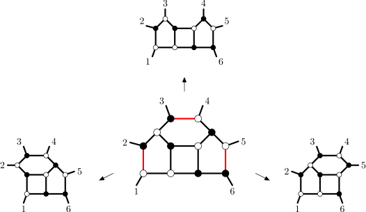
Figure 9: Decaying the six-point NMHV top-cell into three BCFW-channels.

For the undeformed amplitude, it was pointed out in ref. [17] that the conditions for Yangian invariance of the top-cell eqn. (4.47) are equivalent to imposing Yangian invariance on the three channels eqns. (4.46). Thus, Yangian invariance is compatible with decaying the top-cell into individual BCFW channels as long as no deformation is present.

Considering a deformed amplitude, there seems to be an apparent clash: while imposing Yangian invariance on the top-cell leaves six free deformation parameters, demanding Yangian invariance for the three BCFW channels simultaneously leads to only three free deformation parameters:

$$u_{5}\,=u_{4}\ ,\qquad u_{2}\,=u_{3}\ ,\qquad u_{1}\,=u_{6}\ .$$ (4.48)

The resolution is simple: taking a residue of the top-cell, that is “removing a line from the graph in fig. 9” is possible only if there is no flow of central charge along the line to be removed. The three conditions for the simultaneous vanishing of the central charges along the red lines delivers the three additional conditions leading to eqn. (4.48).

What is the analogue of this construction in the $\mathrm{R}$-operator language? In subsec. 3.5 it was discussed that there are exactly six different NMHV Yangian invariants with six external legs, which are listed in eqn. (3.5). As pointed out after eqn. (LABEL:eq:6ptcentralcharges), the three eigenfunctions corresponding to the BCFW channels in eqn. (4.46), $\mathcal{Y}_{1}^{(6)}$, $\mathcal{Y}_{3}^{(6)}$ and $\mathcal{Y}_{5}^{(6)}$, have different central charges, and thus different eigenvalues. Since a sum of Yangian invariants is only well-defined if all of them belong to the same eigenspace of the monodromy matrix, one has to identify the spectral parameters as in eqn. (3.86). This is exactly the condition in eqn. (4.48).

Thus ensuring Yangian invariance by demanding the BCFW channels to be eigenstates of the monodromy matrix is not sufficient: if a deformed amplitude is composed from several deformed Yangian invariants, one has to ensure that they all are in the same eigenspace.

4.5 A peek at the seven-point NMHV amplitude

In order to show the validity of the $\mathrm{R}$-operator formalism, let us consider a more difficult example: the seven-point NMHV amplitude. The on-shell graphs derived from a standard BCFW-decomposition employing a shift of legs $1$ and $7$ correspond to the following strings of R-operators:

$$\mathrm{R}_{76}\,\mathrm{R}_{71}\,\mathrm{R}_{32}\,\mathrm{R}_{12}\,\mathrm{R}_{21}\,\mathrm{R}_{23}\,\mathrm{R}_{61}\,\mathrm{R}_{34}\,\mathrm{R}_{53}\,\mathrm{R}_{36}\,\cdot\delta_{\text{-}1}\delta_{2}\delta_{3}\delta_{\text{-}4}\delta_{5}\delta_{\text{-}6}\delta_{7}\ ,$$ (4.49)

$$\mathrm{R}_{76}\,\mathrm{R}_{71}\,\mathrm{R}_{16}\,\mathrm{R}_{12}\,\mathrm{R}_{21}\,\mathrm{R}_{23}\,\mathrm{R}_{61}\,\mathrm{R}_{34}\,\mathrm{R}_{53}\,\mathrm{R}_{36}\,\cdot\delta_{\text{-}1}\delta_{2}\delta_{3}\delta_{\text{-}4}\delta_{5}\delta_{\text{-}6}\delta_{7}\ ,$$

$$\mathrm{R}_{76}\,\mathrm{R}_{71}\,\mathrm{R}_{16}\,\mathrm{R}_{32}\,\mathrm{R}_{21}\,\mathrm{R}_{23}\,\mathrm{R}_{61}\,\mathrm{R}_{34}\,\mathrm{R}_{53}\,\mathrm{R}_{36}\,\cdot\delta_{\text{-}1}\delta_{2}\delta_{3}\delta_{\text{-}4}\delta_{5}\delta_{\text{-}6}\delta_{7}\ ,$$

$$\mathrm{R}_{43}\,\mathrm{R}_{65}\,\mathrm{R}_{54}\,\mathrm{R}_{43}\,\mathrm{R}_{56}\,\mathrm{R}_{67}\,\mathrm{R}_{16}\,\mathrm{R}_{23}\,\mathrm{R}_{42}\,\mathrm{R}_{26}\,\cdot\delta_{1}\delta_{2}\delta_{\text{-}3}\delta_{4}\delta_{5}\delta_{\text{-}6}\delta_{\text{-}7}\ ,$$

$$\mathrm{R}_{23}\,\mathrm{R}_{45}\,\mathrm{R}_{34}\,\mathrm{R}_{54}\,\mathrm{R}_{56}\,\mathrm{R}_{64}\,\mathrm{R}_{67}\,\mathrm{R}_{16}\,\mathrm{R}_{32}\,\mathrm{R}_{26}\,\cdot\delta_{1}\delta_{2}\delta_{3}\delta_{\text{-}4}\delta_{5}\delta_{\text{-}6}\delta_{\text{-}7}\ ,$$

$$\mathrm{R}_{45}\,\mathrm{R}_{56}\,\mathrm{R}_{71}\,\mathrm{R}_{76}\,\mathrm{R}_{43}\,\mathrm{R}_{53}\,\mathrm{R}_{36}\,\mathrm{R}_{73}\,\mathrm{R}_{31}\,\mathrm{R}_{32}\,\cdot\delta_{\text{-}1}\delta_{\text{-}2}\delta_{3}\delta_{4}\delta_{5}\delta_{\text{-}6}\delta_{7}\,.$$

We have checked that the combination of the above channels does indeed yield the seven-point NMHV superamplitude by comparing with the explicit expressions in [25]. In addition, we performed automated tests and found complete agreement with the results obtained from the Mathematica package GGT described in ref. [40].

While the tree-amplitude is a nontrivial check, one can ask, whether it is possible to obtain all box coefficients for the one-loop seven-point NMHV spelled out in ref. [41] from the top-cell in the $\mathrm{R}$-formalism. Finding the BCFW-channels refers to determining all codimension-two boundaries of the top-cell which – in turn – amounts to omitting two $\mathrm{R}$’s in a suitable representation of the top-cell. A suitable representation reads

$$\mathrm{R}_{65}\,\mathrm{R}_{76}\,\mathrm{R}_{71}\,\mathrm{R}_{54}\,\mathrm{R}_{65}\,\mathrm{R}_{43}\,\mathrm{R}_{45}\,\mathrm{R}_{61}\,\mathrm{R}_{15}\,\mathrm{R}_{41}\,\mathrm{R}_{13}\,\mathrm{R}_{21}\,\cdot\delta_{\text{-}1}\,\delta_{2}\,\delta_{\text{-}3}\,\delta_{4}\,\delta_{\text{-}5}\,\delta_{6}\,\delta_{7}\,$$ (4.50)

and leads to 66 $\mathrm{R}$-chains of length 10. While some of them do not contain all seven indices, and thus do not connect all particles, others do not allow to solve the integral for general kinematics (see subsec. 4.1 for a discussion). Discarding those, one is left with $20$ valid channels, which turn out to deliver a spanning set for all box coefficients calculated in ref. [41].

5 Conclusions

In this article we have explored the $\mathrm{R}$-operator formalism introduced in ref. [18]. We have elucidated the underlying algebraic structures that are related to the Yangian algebra of $\mathfrak{gl}(4|4)$. In particular, considering the S- and R-matrix in the fundamental and functional representation implies the forms of the Lax-operator $\mathrm{L}$ and the R-operator $\mathrm{R}$ in eqns. (3.26) and (3.27), respectively. Via the monodromy matrix $\mathrm{T}$ (3.52), the Lax operator then generates the generators of the Yangian symmetry of $n$-particle states. In this language, Yangian invariants are defined to be eigenfunctions of the monodromy matrix.

One simple eigenfunction of the monodromy matrix is given by a product of $\delta$-functions in the spinor-helicity variables (3.54). From this ground state we can generate Yangian invariants by acting on it with a sequence of R-operators. From the Yang–Baxter equation (3.32) relating $\mathrm{R}$ and $\mathrm{L}$, we see that functions of this form naturally give rise to eigenfunctions.

It would be extremely interesting to derive the explicit expressions of the L- and R-operator from the universal R-matrix. Our discussion in sec. 3 indicates that there is a universal R-matrix underlying this construction of Yangian invariants. It would already be useful to explicitly work out the constructions for $\mathfrak{gl}(2)$ or $\mathfrak{gl}(1|1)$ to gain deeper insights in the algebraic structures that are involved.

We have classified all eigenstates up to six particles and we found that to each Yangian invariant in $\mathcal{N}=4$ sYM there corresponds a unique eigenfunction of the monodromy matrix. Furthermore, each Yangian invariant is determined by its central charges, which are of the form of a difference between spectral parameters (3.90). Using this identity, the central charges can be related to permutations, which establishes a bijection between permutations and Yangian invariants.

Subsequently, we have been identifying the maps between the $\mathrm{R}$-operator formulation of Yangian invariants and their formulations in terms on on-shell graphs and permutations. All properties of Yangian invariants as well as those of the amplitudes built thereof can be given an immediate interpretation: while cyclicity, reflection and flip of parity are very natural in the $\mathrm{R}$-operator language, constraints on possible deformation parameters are realised by demanding an Yangian-invariant object to be an eigenstate of the monodromy matrix, which is built from Lax-operators. The result for building amplitudes with Yangian-invariant deformations is in agreement with [17]: Yangian-invariant deformations are not compatible with the BCFW-construction of amplitudes.

The $\mathrm{R}$-operator language bridges the gap between the common formulations of scattering amplitudes and the formalism employed in integrable systems. The relation becomes even more evident in ref. [22].

There is, however, a drawback of the $\mathrm{R}$-operator formalism: the construction is based on evaluating integrals on the support of delta functions. Since one can perform the integrals in any succession, and the arguments of the delta functions can be reversed without modifying the physical situation, there is a sign ambiguity related to each Yangian invariant. Although the formalism delivers the Yangian invariants, it is not clear, in which way they need to be combined. Naturally, this can be fixed by demanding the vanishing of spurious poles, nevertheless, one would rather like to have a purely constructional method. One way to realise this could be an algebraic condition singling out BCFW-channels.

While the current article deals with tree amplitudes exclusively, there is hope for extending the formalism to loop amplitudes. Similar to the forward-limit construction in [14], one will have to identify two legs in order to build the $\mathrm{R}$-chain corresponding to a loop-amplitude. Nevertheless, the integration procedure will not be as straightforward as in the tree-level case, because infrared divergences will appear.

Acknowledgements.

We would like to thank Niklas Beisert, James Drummond, Henrik Johansson, Nils Kanning, Yumi Ko, Jan Plefka, Matthias Staudacher and Cristian Vergu for useful discussions. The work of MdL and MR is partially supported by grant no. 200021-137616 from the Swiss National Science Foundation.

Appendix A Momentum twistors and algebraic approach

In ref. [18], the authors proposed an extension of their algebraic approach to scattering amplitudes to the momentum twistor formulation. They define the $\mathrm{R}_{ij}$-operator acting on the space of functions on momentum twistor space as

$$\mathrm{R}_{ij}(u)\cdot\mathcal{F}\bigl{(}\mathcal{W}_{i},\mathcal{W}_{j}\bigr{)}:=\int\frac{\mathrm{d}z}{z^{1+u}}\,\mathcal{F}\bigl{(}\mathcal{W}_{i}-z\mathcal{W}_{j},\mathcal{W}_{j}\bigr{)}\ ;$$ (A.1)

in the following we will always consider $\mathrm{R}$-operators whose spectral parameter $u$ is set to zero. Subsequently, the authors show that the following identity holds:

$$\mathcal{I}=\mathrm{R}_{34}\mathrm{R}_{23}\mathrm{R}_{12}\mathrm{R}_{*1}\delta^{4|4}(\mathcal{W}_{*})=[*,1,2,3,4]\ .$$ (A.2)

An important remark is due here: this is not the formulation one obtains from translating the on-shell superspace approach directly into momentum twistor variables. While a first proof of this is the non-locality of the BCFW shift in momentum twistor space (whereas this $\mathrm{R}$-operator acts on two sites only), another proof is the fact that the vacuum of the on-shell superspace approach does not translate into anything nice in momentum twistor space. While this could be a formulation equivalent to the Grassmannian formula in momentum twistor space, the dictionary is not direct.

The explicit computation of (A.2) is straightforward. From

$$\mathcal{I}=\int\biggl{[}\prod_{i=1}^{4}\frac{\mathrm{d}z_{i}}{z_{i}}\biggr{]}\,\delta^{4|4}(\mathcal{W}_{*}-z_{1}\mathcal{W}_{1}+z_{1}z_{2}\mathcal{W}_{2}-z_{1}z_{2}z_{3}\mathcal{W}_{3}+z_{1}z_{2}z_{3}z_{4}\mathcal{W}_{4})$$ (A.3)

we can change variables to

$$a_{i}:=(-1)^{i+1}\prod_{k=1}^{i}z_{k}$$ (A.4)

and the (inverse) Jacobian is $|\mathrm{det}\,J^{-1}|=a_{1}a_{2}a_{3}$. This leads to

$$\mathcal{I}=\int\biggl{[}\prod_{i=1}^{4}\frac{\mathrm{d}a_{i}}{a_{i}}\biggr{]}\delta^{4|4}(\mathcal{W}_{*}-\sum_{i}a_{i}\mathcal{W}_{i})\ .$$ (A.5)

We can now solve the integrals by localising them on the support of the bosonic delta functions. In order to do so, we rewrite the bosonic delta functions by dotting into the arguments $\epsilon^{\alpha}(1,2,3,\bullet),\epsilon^{\alpha}(1,2,4,\bullet),\epsilon^{\alpha}(1,3,4,\bullet),\epsilon^{\alpha}(2,3,4,\bullet)$:

$$\delta^{4}(W_{*}-\sum_{i}W_{i})=\frac{1}{\langle 1234\rangle}\delta\biggl{(}a_{1}-\frac{\langle*234\rangle}{\langle 1234\rangle}\biggr{)}\delta\biggl{(}a_{2}-\frac{\langle*134\rangle}{\langle 1234\rangle}\biggr{)}\delta\biggl{(}a_{3}-\frac{\langle*124\rangle}{\langle 1234\rangle}\biggr{)}\delta\biggl{(}a_{4}-\frac{\langle*123\rangle}{\langle 1234\rangle}\biggr{)}\ .$$ (A.6)

The result reads

$$\mathcal{I}=\frac{\delta^{0|4}\bigl{(}\langle 1234\rangle\chi_{*}+\langle 234*{}\rangle\chi_{1}+\langle 34*{}1\rangle\chi_{2}+\langle 4*12\rangle\chi_{3}+\langle*123\rangle\chi_{4}\bigr{)}}{\langle 1234\rangle\langle 234*\rangle\langle 34*1\rangle\langle 4*12\rangle\langle*123\rangle}\equiv[*,1,2,3,4]\ .$$ (A.7)

This result is not unexpected, because the expression in eqn. (A.5) is – if we allow ourselves to be not too rigorous with the integration measure – the form of the NMHV $\mathcal{R}$-invariants as an integral over $\mathbb{CP}^{5}$ first introduced by Mason and Skinner in ref. [42]. The construction of eqn. (A.2) therefore leads “trivially” to the correct NMHV $\mathcal{R}$-invariant.

An interesting problem is to understand whether it is possible to extend this construction to higher-level $\mathcal{R}$-invariants. It is possible in fact to express dual superconformal invariants in terms of residue integrals over suitable Grassmannian manifolds (as shown in ref. [42] and then exploited in ref. [12] to show the equivalence between the ordinary Grassmannian formulation and the dual Grassmannian formulation). However, the problem is that there is no interpretation of the shift in eqn. (A.1), neither in BCFW nor in Risager form. It would be interesting to analyse whether it is possible to find a map from MHV diagrams in momentum-twistor space to these $\mathrm{R}$-operators, analogous to the correspondence to on-shell graphs (and BCFW channels) described in the main part of the article.

Nevertheless, it is possible to “engineer” a set of $\mathrm{R}$-operators that lead to the expression for $k=4$ $\mathcal{R}$-invariants (eqn. (55) in ref. [42])

$$\mathcal{R}_{k,n}:=\frac{1}{(2\pi i)^{(k-2)(n-k-2)}}\oint_{\mathrm{\Gamma}\subset G(k-2,n)}\!\!\!\!\!\mathrm{d}\mu\,\prod_{i=1}^{k-2}\delta^{4|4}\biggl{(}\sum_{j=1}^{n}C_{ij}\mathcal{W}_{j}\biggr{)}\ ,$$ (A.8)

where $C_{lj}$ is the $(k-2)\times n$ matrix representing a point on $G(k-2,n)$ and the measure is the “usual” measure for amplitude-related Grassmannian integrals, that is

$$\mathrm{d}\mu=\frac{\mathrm{d}^{k\times n}c_{ab}}{\mathrm{Vol}[\mathrm{GL}(k)]}\frac{1}{(12\dots k)(23\dots k+1)\dots(n\dots k-1)}\ .$$ (A.9)

The easiest example with $k=4$ is the $6$-point $\mathcal{R}$-invariant, since the corresponding integral is completely localised on the support of the delta functions, and should lead to the $\mathrm{N}^{2}\mathrm{MHV}$ (or $\overline{\mathrm{MHV}}$) $6$-point amplitude. We can show that the correct expression is

$$\mathrm{R}^{(8)}_{34}\,\mathrm{R}^{(7)}_{23}\,\mathrm{R}^{(6)}_{16}\,\mathrm{R}^{(5)}_{34}\,\mathrm{R}^{(4)}_{63}\,\mathrm{R}^{(3)}_{56}\,\mathrm{R}^{(2)}_{25}\,\mathrm{R}^{(1)}_{15}\,\delta^{4|4}(\mathcal{W}_{1})\,\delta^{4|4}(\mathcal{W}_{2})\ ,$$ (A.10)

where the superscript $(i)$ indicates that the integral associated to this $\mathrm{R}$-operator is over the variable $z_{i}$. It corresponds to the integral

$$I=\int\biggl{[}\prod_{i=1}^{8}\frac{\mathrm{d}z_{i}}{z_{i}}\biggr{]}\delta^{4|4}\Bigl{[}\mathcal{W}_{1}-z_{1}\mathcal{W}_{5}-z_{1}z_{3}z_{4}\mathcal{W}_{3}+(z_{1}z_{3}-z_{6})\mathcal{W}_{6}+z_{1}z_{3}z_{4}(z_{5}+z_{8})\mathcal{W}_{4}\Bigr{]}\times$$ (A.11)

$$\delta^{4|4}\Bigl{[}\mathcal{W}_{2}-z_{2}\mathcal{W}_{5}+z_{2}z_{3}\mathcal{W}_{6}+(-z_{2}z_{3}z_{4}-z_{7})\mathcal{W}_{3}+[z_{2}z_{3}z_{4}(z_{5}+z_{8})+z_{7}z_{8}]\mathcal{W}_{4}\Bigr{]}\ .$$

With the obvious change of variables

$$c_{ij}:=(\text{coefficient of }\mathcal{W}_{j}\text{ in the $i$-th delta function})$$

one obtains

$$I=\int\frac{\mathrm{d}^{2\times 4}c_{ab}}{c_{13}c_{26}(c_{13}c_{24}-c_{14}c_{23})(c_{15}c_{24}-c_{14}c_{25})(c_{15}c_{26}-c_{16}c_{25})}\prod_{i=1,2}\delta^{4|4}(\sum_{j=1}^{6}c_{ij}\mathcal{W}_{j})\ ,$$ (A.12)

which is exactly eqn. (A.8) with the $\mathrm{GL}(2)$ freedom used to fix the first two columns of $c_{ab}$ to the identity, that is

$$c_{ab}=\begin{pmatrix}1&0&c_{13}&c_{14}&c_{15}&c_{16}\\ 0&1&c_{23}&c_{24}&c_{25}&c_{26}\end{pmatrix}\ .$$ (A.13)

This is, however, an ad hoc construction, engineered to qualitatively match the integral description of R-invariants of ref. [42]. What conclusions can thus be drawn from here?

First of all, it is not clear in this momentum-twistor approach what the vacuum state $\delta^{4|4}(\mathcal{W})$ is, even though it is pretty clear that one such state should be associated to each off-shell leg in a given MHV diagram. It also seems that the specific choice of a vacuum corresponds to a particular way of fixing the $\mathrm{GL}(k)$ redundancy in the integral over the Grassmannian.

Secondly, it would be nice to have a map from MHV diagrams (which have a very natural description in momentum twistor space [43]) to $\mathrm{R}$-chains acting on momentum-twistor space, but it is currently not clear, whether this map exists. Moreover, the translation seems to get rather complicated starting from the NNMHV level, since the MHV diagrams in the expansion have an increasingly complicated topology.

References

- [1] L. Brink, J. H. Schwarz and J. Scherk, “Supersymmetric Yang-Mills theories”, Nucl.Phys. B121, 77 (1977).
- [2] F. Gliozzi, J. Scherk and D. I. Olive, “Supersymmetry, supergravity theories and the dual spinor model”, Nucl.Phys. B122, 253 (1977).
- [3] P. S. Howe, K. Stelle and P. Townsend, “Miraculous ultraviolet cancellations in supersymmetry made manifest”, Nucl.Phys. B236, 125 (1984).
- [4] L. Brink, O. Lindgren and B. E. Nilsson, “N=4 Yang-Mills theory on the light cone”, Nucl.Phys. B212, 401 (1983).
- [5] L. Brink, O. Lindgren and B. E. Nilsson, “The ultraviolet finiteness of the N=4 Yang-Mills theory”, Phys.Lett. B123, 323 (1983).
- [6] S. Mandelstam, “Light cone superspace and the finiteness of the N=4 model”.
- [7] J. Drummond, J. Henn, G. Korchemsky and E. Sokatchev, “Dual superconformal symmetry of scattering amplitudes in N=4 super-Yang-Mills theory”, Nucl.Phys. B828, 317 (2010), arxiv:0807.1095.
- [8] J. M. Drummond, J. M. Henn and J. Plefka, “Yangian symmetry of scattering amplitudes in N=4 super Yang-Mills theory”, JHEP 0905, 046 (2009), arxiv:0902.2987.
- [9] N. Arkani-Hamed, F. Cachazo, C. Cheung and J. Kaplan, “A duality for the S matrix”, JHEP 1003, 020 (2010), arxiv:0907.5418.
- [10] N. Arkani-Hamed, F. Cachazo and J. Kaplan, “What is the simplest Quantum Field Theory?”, JHEP 1009, 016 (2010), arxiv:0808.1446.
- [11] N. Arkani-Hamed, J. L. Bourjaily, F. Cachazo, S. Caron-Huot and J. Trnka, “The all-loop integrand for scattering amplitudes in planar N=4 SYM”, JHEP 1101, 041 (2011), arxiv:1008.2958.
- [12] N. Arkani-Hamed, F. Cachazo and C. Cheung, “The Grassmannian origin of dual superconformal invariance”, JHEP 1003, 036 (2010), arxiv:0909.0483.
- [13] N. Arkani-Hamed, J. Bourjaily, F. Cachazo and J. Trnka, “Unification of residues and Grassmannian dualities”, JHEP 1101, 049 (2011), arxiv:0912.4912.
- [14] N. Arkani-Hamed, J. L. Bourjaily, F. Cachazo, A. B. Goncharov, A. Postnikov et al., “Scattering amplitudes and the positive Grassmannian”, arxiv:1212.5605.
- [15] L. Ferro, T. Lukowski, C. Meneghelli, J. Plefka and M. Staudacher, “Harmonic R-matrices for scattering amplitudes and spectral regularization”, Phys.Rev.Lett. 110, 121602 (2013), arxiv:1212.0850.
- [16] L. Ferro, T. Lukowski, C. Meneghelli, J. Plefka and M. Staudacher, “Spectral parameters for scattering amplitudes in N=4 super Yang-Mills theory”, arxiv:1308.3494.
- [17] N. Beisert, J. Broedel and M. Rosso, “On Yangian-invariant regularisation of deformed on-shell diagrams in N=4 super-Yang-Mills theory”, arxiv:1401.7274.
- [18] D. Chicherin, S. Derkachov and R. Kirschner, “Yang-Baxter operators and scattering amplitudes in N=4 super-Yang–Mills theory”, arxiv:1309.5748.
- [19] D. Chicherin and R. Kirschner, “Yangian symmetric correlators”, Nucl.Phys. B877, 484 (2013), arxiv:1306.0711, http://arxiv.org/abs/arXiv:1306.0711.
- [20] D. Nandan and C. Wen, “Generating All Tree Amplitudes in N=4 SYM by Inverse Soft Limit”, JHEP 1208, 040 (2012), arxiv:1204.4841.
- [21] R. Frassek, N. Kanning, Y. Ko and M. Staudacher, “Bethe Ansatz for Yangian Invariants: Towards Super Yang-Mills Scattering Amplitudes”, arxiv:1312.1693.
- [22] N. Kanning, T. Lukowski and M. Staudacher, “A Shortcut to General Tree-level Scattering Amplitudes in N=4 SYM via Integrability”, arxiv:1403.3382.
- [23] V. Nair, “A current algebra for some gauge theory amplitudes”, Phys.Lett. B214, 215 (1988).
- [24] E. Witten, “Perturbative gauge theory as a string theory in twistor space”, Commun.Math.Phys. 252, 189 (2004), hep-th/0312171.
- [25] R. Britto, F. Cachazo and B. Feng, “New recursion relations for tree amplitudes of gluons”, Nucl.Phys. B715, 499 (2005), hep-th/0412308.
- [26] R. Britto, F. Cachazo, B. Feng and E. Witten, “Direct proof of tree-level recursion relation in Yang-Mills theory”, Phys.Rev.Lett. 94, 181602 (2005), hep-th/0501052.
- [27] A. Brandhuber, P. Heslop and G. Travaglini, “A note on dual superconformal symmetry of the N=4 super Yang-Mills S-matrix”, Phys.Rev. D78, 125005 (2008), arxiv:0807.4097.
- [28] A. Postnikov, “Total positivity, Grassmannians, and networks”, math/0609764.
- [29] N. MacKay, “Introduction to Yangian symmetry in integrable field theory”, Int.J.Mod.Phys. A20, 7189 (2005), hep-th/0409183.
- [30] N. Beisert and B. U. Schwab, “Bonus Yangian Symmetry for the Planar S-Matrix of N=4 Super Yang-Mills”, Phys.Rev.Lett. 106, 231602 (2011), arxiv:1103.0646.
- [31] N. Beisert and M. de Leeuw, “The RTT-Realization for the Deformed Yangian”, arxiv:1401.7691.
- [32] V. G. Drinfel’d, “Hopf algebras and the quantum Yang-Baxter equation”, Sov. Math. Dokl. 32, 254 (1985).
- [33] V. G. Drinfel’d, “Quantum groups”, J. Math. Sci. 41, 898 (1988).
- [34] S. Khoroshkin and V. Tolstoi, “Yangian double and rational R matrix”, hep-th/9406194.
- [35] L. A. Takhtajan and L. D. Faddeev, “The quantum method of the inverse problem and the Heisenberg XYZ model”, Russ.Math.Surveys 34, 11 (1979).
- [36] P. P. Kulish and E. K. Sklyanin, “On the solution of the Yang-Baxter equation”, J.Sov.Math. 19, 1596 (1982).
- [37] L. D. Faddeev, N. Yu. Reshetikhin and L. Takhtajan, “Quantization of Lie groups and Lie algebras”, Leningrad Math.J. 1, 193 (1990).
- [38] S. Khoroshkin, D. Lebedev and S. Pakuliak, “Intertwining operators for the central extension of the Yangian double”, q-alg/9602030.
- [39] S. Khoroshkin, “Central extension of the Yangian double”, q-alg/9602031.
- [40] L. J. Dixon, J. M. Henn, J. Plefka and T. Schuster, “All tree-level amplitudes in massless QCD”, JHEP 1101, 035 (2011), arxiv:1010.3991.
- [41] Z. Bern, V. Del Duca, L. J. Dixon and D. A. Kosower, “All non-maximally-helicity-violating one-loop seven-gluon amplitudes in N=4 super-yang-Mills theory”, Phys.Rev. D71, 045006 (2005), hep-th/0410224.
- [42] L. Mason and D. Skinner, “Dual Superconformal Invariance, Momentum Twistors and Grassmannians”, JHEP 0911, 045 (2009), arxiv:0909.0250.
- [43] M. Bullimore, L. Mason and D. Skinner, “MHV Diagrams in Momentum Twistor Space”, JHEP 1012, 032 (2010), arxiv:1009.1854.