Pattern formation in systems with multiple delayed feedbacks

Abstract

Dynamical systems with complex delayed interactions arise commonly when propagation times are significant, yielding complicated oscillatory instabilities. In this Letter, we introduce a class of systems with multiple, hierarchically long time delays, and using a suitable space-time representation we uncover features otherwise hidden in their temporal dynamics. The behaviour in the case of two delays is shown to ”encode” two-dimensional spiral defects and defects turbulence. A multiple scale analysis sets the equivalence to a complex Ginzburg-Landau equation, and a novel criterium for the attainment of the long-delay regime is introduced. We also demonstrate this phenomenon for a semiconductor laser with two delayed optical feedbacks.

Systems with time delays are common in many fields, ranging from optics (e.g. laser with feedback Li et al. (2011); Zamora-Munt et al. (2010); Giacomelli et al. (2012); Soriano et al. (2013)), vehicle systems Szalai and Orosz (2013), to neural networks Izhikevich (2006), information processing Appeltant et al. (2011), and many others Erneux (2009). A finite propagation velocity of the information introduces in such systems a new relevant scale, which is comparable or higher than the intrinsic timescales. It has been shown that the complexity of such systems, e.g. the dimension of attractors, is finite and it grows linearly with time delay Farmer (1982); moreover, the spectrum of Lyapunov exponents approaches a continuous limit for long delay Giacomelli et al. (1995); Heiligenthal et al. (2011); D’Huys et al. (2013). As a result, in this case essentially high-dimensional phenomena can occur such as spatio-temporal chaos Giacomelli and Politi (1996), square waves Erneux (2009), Eckhaus destabilization Wolfrum and Yanchuk (2006), or coarsening Giacomelli et al. (2012). In the above mentioned situations, the system involves one long delay, which can be interpreted as the size of a one-dimensional, spatially extended system Arecchi et al. (1992); Giacomelli and Politi (1996). This approach has proven to be instrumental in explaining new phenomena in systems with time delays Giacomelli et al. (1994); Larger et al. (2013).

In this Letter, we show that many new challenging problems arise when a system is subject to several delayed feedbacks acting on different scales. In contrast to the single delay situation, essentially new phenomena occur, related to higher spatial dimensions involved in the dynamics, such as spirals or defect turbulence. As an illustration, we consider a specific physical system, namely, a model of a semiconductor laser with two optical feedbacks.

A simple paradigmatic setup for the multiple delays case is the following system

$$\dot{z}=az+bz_{\tau_{1}}+cz_{\tau_{2}}+dz|z|^{2}.$$ (1)

Eq. (1) describes a very general situation: the interplay of the oscillatory instability (Hopf bifurcation) and two delayed feedbacks $z_{\tau_{i}}=z(t-\tau_{i})$, that we consider acting on different timescales $1\ll\tau_{1}\ll\tau_{2}$. The variable $z(t)$ is complex, and the parameters $a$, $b$, and $c$ determine the instantaneous, $\tau_{1}$-, and $\tau_{2}$-feedback rates, respectively. The instantaneous part of the system (without feedback) is known as the normal form for the Hopf bifurcation.

The following basic questions arise: what kind of new phenomena can be observed in systems with several delayed feedbacks? Can one relate the dynamics of such systems to spatially extended systems with several spatial dimensions? In the case of positive answer, under which conditions? Is it possible to observe such essentially 2D phenomena as, e.g., spiral waves in purely temporal delay systems (1), which obey the causality principle with respect to the time? In this Letter we address the above questions. In particular, we show that such inherently 2D patterns as spiral defects or defect turbulence Chaté and Manneville (1996), are typical behaviors of system (1). Moreover, they can be generically found in a semiconductor laser model with two optical feedbacks.

We start with numerical examples. Figures 1 and 2 show solutions of Eq. (1) for two different parameter choices. Time series in Figs. 1(a) and 2(a) exhibit oscillations on different timescales related approximately to the delay times. However, an appropriate spatio-temporal representation of the data [see e.g. Figs. 1(b-c) and 2(b-c)] reveals clearly the nature of the dynamical behaviors. More details on the appropriate spatio-temporal representation of these purely temporal data will be given later, but one can readily observe that the first case corresponds to a (frozen) spiral (FS) defects solution, see Fig. 1(b,c). The positions of the two coexisting spiral defects are shown by the dots, where the level lines for the phase meet. Consequently, the phase is not defined there and $|z|=0$. The solution shown in Fig. 2 corresponds instead to the defect turbulence (DT) regime. One can observe that the modulation of the amplitude $\left|z(t)\right|$ starts to approach the zero level in a random-like manner. In this case, the corresponding spatial representation (see Fig. 2(b,c)) reveals DT, i.e. the non-regular motions of the spiral defects. The plots correspond to snapshots in time.

In the following, we explain why the observed behaviors are typical and show how to relate the dynamics of (1) to the complex Ginzburg-Landau equation on a 2D spatial domain. In particular, we show that the function $z(t)$ on the time interval of the length $\tau_{2}$ corresponds to a snapshot of a 2D spatial function $\Phi(x,y)$. The corresponding pseudo-spatial coordinates $x$ and $y$ introduced later by Eq. (3) are different scales of the time. We will show, that the parameters of (1) leading to the FS (resp. DT) can be mapped uniquely to the parameters of the Ginzburg-Landau system, for which the same phenomenologies are observed Chaté and Manneville (1996). This behavior is observed robustly for all tested random initial conditions for an interval of parameters.

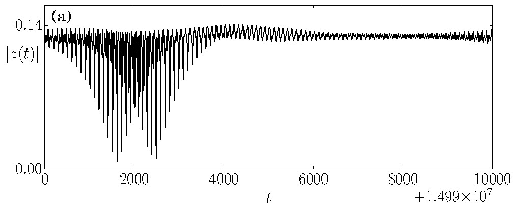
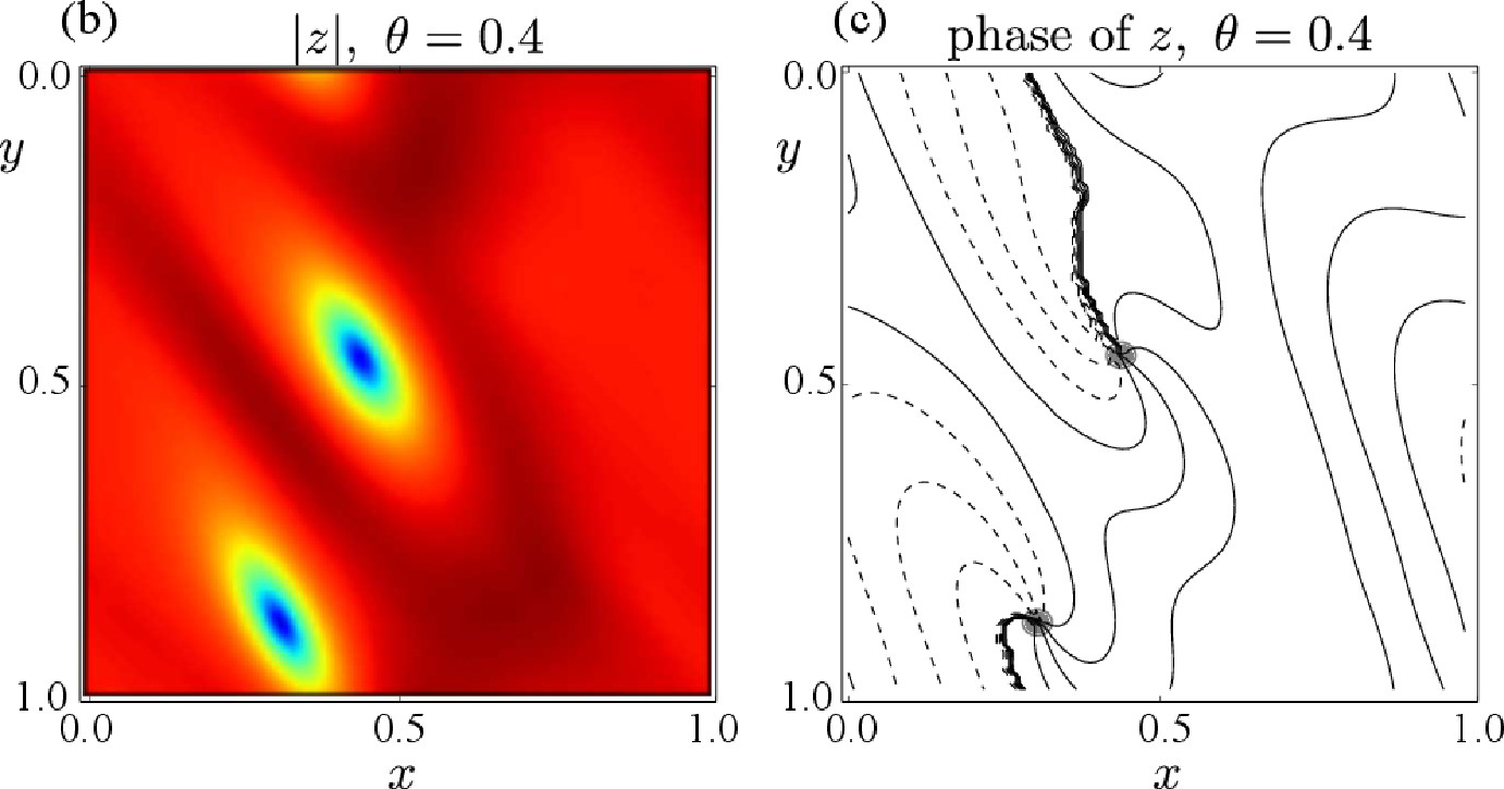
Figure 1: Spiral defects in system with delays (1). (a) Typical time series of the absolute value $|z(t)|$. Spatio-temporal representation of the time series using pseudo-space coordinates (3) reveals the spiral defects: (b) Snapshot of the spatial profile in the pseudo-space coordinates $(x,y)$ for $\theta_{0}=0.4$. (c) Constant level lines for the phase of $z$. Circles denote the positions of defects. Parameters: $a=-0.985$, $b=0.4$, $c=0.6$ (corresponding to $P=0.015$), $d=-0.75+i$, $\tau_{1}=100$, and $\tau_{2}=10000$. Initial conditions are chosen randomly.

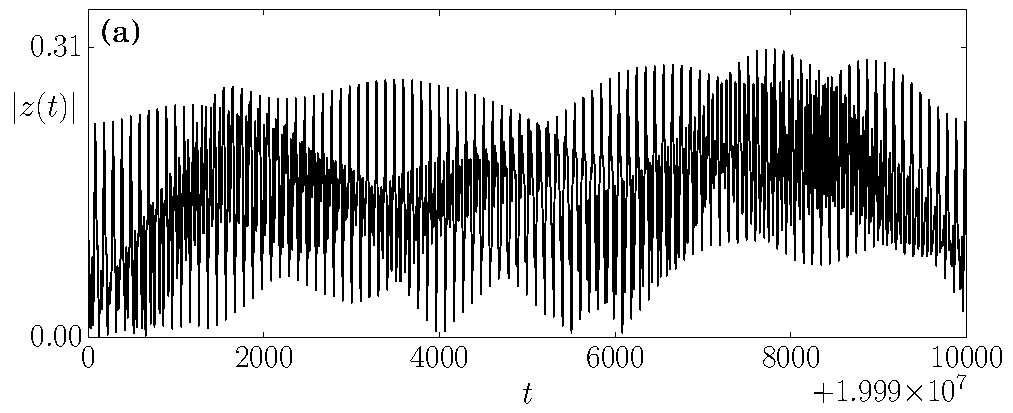
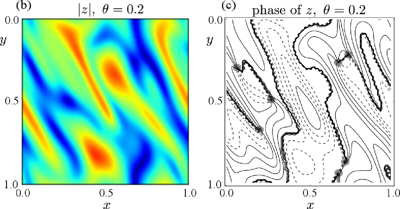
Figure 2: Defects turbulence in delayed system (1). Same as in Fig. 1 for different value of $d=-0.1+i$. Spatio-temporal representation in (b) and (c) reveals defects turbulence.

Normal form equation. The long time delay $\tau_{1}$ can be written as $\tau_{1}=1/\varepsilon$ with a small positive parameter $\varepsilon$, and $\tau_{2}=\kappa/\varepsilon^{2}$ with some positive $\kappa$. With such notations, the scale separation $1\ll\tau_{1}\ll\tau_{2}$ is satisfied. Notice that this also gives an indication how one should proceed in the case of more than two delays.

In order to derive a normal form describing universally the dynamics close to the destabilization of system (1), the multiple scale ansatz $z(t):=\varepsilon u\left(\varepsilon t,\varepsilon^{2}t,\varepsilon^{3}t,\varepsilon^{4}t\right)$ is used. More precisely, substituting this ansatz as well as the perturbation parameter $\varepsilon^{2}p=a+|b|+|c|$ in (1), and time delays $\tau_{1}=1/\varepsilon$, $\tau_{2}=\kappa/\varepsilon^{2}$, one obtains several separate solvability conditions for different orders of $\varepsilon$. The resulting equation is the Ginzburg-Landau partial differential equation

$$\Phi_{\theta}=p\Phi+a_{1}\Phi_{x}+a_{2}\Phi_{y}+a_{3}\Phi_{xx}+a_{4}\Phi_{xy}+a_{5}\Phi_{yy}+d\Phi|\Phi|^{2}$$ (2)

for a function $\Phi(\theta,x,y)$, which is related to the solutions of (1) by $z(t)=\varepsilon\Phi\left(\theta,x,y\right)$, where

$$\theta=\varepsilon^{4}\delta t,\quad x=\varepsilon t\left(1-\delta\varepsilon^{2}\right),\quad y=\varepsilon^{2}t\left(1-\left|b\right|\delta\varepsilon\right),$$ (3)

and $\delta=-\left(a+\left|b\right|\right)^{-1}>0$. The new spatial variables $x$ and $y$ are different timescales of the original time $t$, and the new time variable $\theta$ is the slow time scale $\varepsilon^{4}t$. Therefore, the new spatial and temporal variables can be called pseudo-space and pseudo-time. The coefficients in (2) are $a_{1}=a_{4}=\delta|b|$, $a_{2}=-1+\delta\left|b\right|^{2}$, $a_{3}=\delta/2$, and $a_{5}=-\delta a\left|b\right|/2$. One can note that the diffusion coefficients in this equation are real. The dynamics of (2) is known Chaté and Manneville (1996); Aranson and Kramer (2002) to possess various phase transitions, FS (e.g. for $d=-0.75+i$), and DT (e.g. for $d=-0.1+i$). We found a good correspondence between the dynamics of systems (2) and (1), taking into account the relation (3) between them. Although a systematic parametric investigation is out of the scope of this Letter, the examples of FS and DT for the above mentioned parameter values shown in Figs. 1 and 2 are well reproduced. Moreover, the observed dynamics is robust with respect to small variations of parameters. We remark that the observed phenomena are not possible in systems with one time delay, since they arise from the two-dimensional space $(x,y)$ of the normal form equation.

Drift and comoving Lyapunov exponents. The spatial coordinates in (3) can be rewritten as $x=\bar{x}-\delta\bar{u}$ and $y=\bar{y}-|b|\delta\bar{u}$, where $\bar{x}=\varepsilon t$, $\bar{y}=\varepsilon^{2}t$, and $\bar{u}=\varepsilon^{3}t$. As a consequence, we can infer the existence of a (fast) drift along the vector $\mathbf{V}_{d}=(-1,-|b|)$ in the “naive” coordinates $(\bar{x},\bar{y})$. The corrected coordinates (3) eliminate this drift so that the remaining variables are governed by the Ginzburg-Landau equation (2).

The above phenomenon is a consequence of the properties of the maximal comoving (or convective) Lyapunov exponent $\Lambda$ Deissler and Kaneko (1987). In the spherical coordinates $\bar{u}=\rho\cos\alpha$, $\bar{y}=\rho\sin\alpha\cos\beta$, $\bar{x}=\rho\sin\alpha\sin\beta$, it is found that

$$\Lambda(\alpha,\beta)=a\sin\alpha\sin\beta+\big{(}1+\log{(|b|\tan\beta)}\big{)}\sin\alpha\cos\beta\\ +\big{(}1+\log{(|c|\sin\beta\tan\alpha)}\big{)}\cos\alpha.$$ (4)

Details of the calculation will be presented elsewhere. A geometrical interpretation can be introduced using the velocity $\mathbf{V}=(\sin\beta\tan\alpha,\cos\beta\tan\alpha)$, along which the perturbations evolve with a multiplier $e^{\Lambda(\alpha,\beta)}$. The propagation cone’s boundaries can be defined as the set $(\alpha,\beta)$ such that $\Lambda(\alpha,\beta)=0$. The bifurcation point, attained when the maximum of $\Lambda$ is equal to zero, is obtained at $\mathbf{V}=\delta\mathbf{V}_{d}$, corresponding to $(\alpha_{0},\beta_{0})=(\tan^{-1}(-\delta\sqrt{1+|b|^{2}}),\tan^{-1}(|b|^{-1}))$. Note that the direction $\mathbf{V}_{d}$ is also given by the multiscale method above. The above result extends the standard linear stability analysis by indicating the direction along which the destabilization takes place. We notice that the comoving exponent diverges logarithmically close to the axis $\alpha=0$ and $\beta=0$, i.e. instantaneous propagations are forbidden. In the opposite limit, $\alpha\to\pi/2$ (resp. $\beta\to\pi/2$), $\Lambda$ approaches the value for the single delay case $c=0$ ($b=0$). Finally when both $\alpha,\beta\to\pi/2$ (infinite velocity), $\Lambda=a$ and the dynamics is governed by the local term as expected.

On long delay approximation. Concerning the relation between the delay system (1) and the normal form (2), the following questions arise: to what extent the equivalence is founded? Under which conditions the delays are large "enough"? Dynamically, the absence of the anomalous Lyapunov exponents Giacomelli et al. (1995) is required, or, equivalently, the absence of the strong chaos Heiligenthal et al. (2011). Numerically, with the decreasing of delays, the spatio-temporal structures become transients towards a periodic or constant amplitude ($|z|=\mbox{const}$) state. As a matter of fact, a solution of the delay system evolves along the one-parametric line $(\theta(t),x(t),y(t))$ defined by (3) in the pseudo space $(\theta,x,y)$, see Fig. 3(a). In order to have a good correspondence between the solutions of delay system (1) and the normal form through the parametrization (3), the line $(x(t),x(t))$ should wind up the space $(x,y)$ sufficiently densely. In the leading order, this line satisfies $y\approx\varepsilon x$ and it is wrapped periodically at $x=0$ and $x=1$, see Fig. 3(a). The distance between the neighboring branches is $\sim\varepsilon$ which determines the “discretization” level. Thus, high delays imply dense covering of the (pseudo) space plane, as expected in the thermodynamic limit. However, when such density is too small the dynamics changes drastically and the delay system behaves quite differently from the corresponding normal form.

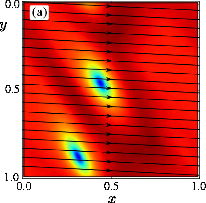
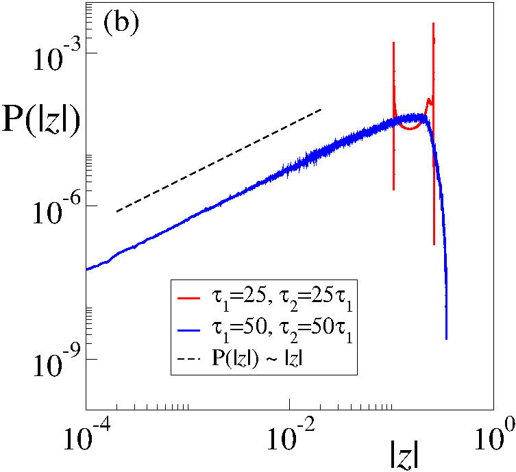
Figure 3: "Small" delays effect. (a) One-parameter curve $x(t),y(t)$ in the pseudo-space determined by (3) for $\varepsilon=0.05$. For larger distances between the branches (smaller delays), the line does not resolve the cores of the spiral of the corresponding GL model. (b) numerical histograms of $|z|$ for the DT regime (parameters as in Fig. 2) for increasing delays values. Histograms for smaller delays (here, $\tau_{1}=25$, $\tau_{2}=25\tau_{1}$) correspond to bounded, periodic solutions with no defects, reached after a transient. A tail in the distribution appears for highers delays (here, $\tau_{1}=50,$ $\tau_{2}=50\tau_{1}$). The dashed line is a reference curve $P(|z|)\sim|z|^{1}$.

To illustrate such a behavior, we present in Fig. 3(b) the analysis of the amplitude $|z|$ statistics in the defect turbulence regime for the model (1). For small delays the dynamics relaxes to a stationary oscillating regime after a transient, with the corresponding histogram showing a shape very close to that obtained from a sinusoidal signal. For higher $\tau$’s , the histogram start displaying a power-law tail $P(|z|)\sim|z|^{1}$ for $|z|\to 0$, indicating the stable appearance of defects and the attainment of the long-delayed regime.

The scaling exponent can be obtained analytically for an arbitrary number of delays and equations. In the DT regime, defects are the spatial points where $|\Phi|=0$ in a $N$-dimensional space ($N$ being the number of delays) and form a set $D$ that we can assume of constant density in space. In our case of $N=2$ these are point defects, for $N=3$ line defects, etc.. In general, it holds that $\mathrm{codim}(D)=2$ in the $N$-dimensional space $\{x_{1},x_{2},..x_{N}\}$ where $\{x_{i}\}$ are the pseudo-spatial coordinates. The delay equation(s) dynamics approaches $D$ along the domain line $L=\{x_{1}(t),x_{2}(t),..x_{N}(t):t\in\mathbb{R}\}$. The vicinity of defects in the pseudo space affects the amplitude statistics of the delay dynamics, which will be depending only on $\mathrm{codim}(D)=2$ and on $\mathrm{dim}(L)=1$. Thus, the scaling exponent does not depend on $N$ or on the number of equations and it can be shown to be equal to $1$.

Semiconductor laser with two optical feedbacks. The results obtained from the study of the normal form (1) are expected to apply to a wide class of physical systems. In the following, we consider a Lang-Kobayashi-type model Lang and Kobayashi (1980) of a single mode semiconductor laser with optical feedback, generalized to a double external cavity configuration:

$$E^{\prime}(t)=(1+i\alpha)n(t)E(t)+\eta_{1}E(t-\tau_{1})+\eta_{2}E(t-\tau_{2}),$$ (5)

$$Tn^{\prime}(t)=J-n(t)-(2n(t)+1)|E(t)|^{2}.$$

$E(t)$ is the complex electric field and $n(t)$ the excess carrier density. The system parameters are the excess pump current $J$, the external cavities round trip times $\tau_{1}$ and $\tau_{2}$ measured in units of the photon lifetime, and the feedback strengths $\eta_{1}$ and $\eta_{2}$. The linewidth enhancement factor $\alpha$ is specific for semiconductor lasers and affects many aspects of their behavior (see e.g. Soriano et al. (2013)). We present here two examples of the dynamics of (5) in the case of $\alpha=2$ and $\alpha=4$. Suitable laser devices can be employed to realize the corresponding experiments; in fact, such range is typical and e.g. measurements in-between have been reported Barland et al. (2005).

In our case, shortly after the destabilization of the ”off-state” $E=0$, a multifrequency oscillating behavior is found, corresponding to FS ($\alpha=2$, Fig. 4(a-b)) or DT ($\alpha=4$, Fig. 4(c)). These regimes are very similar to those shown in Fig. 1 and Fig. 2 respectively. In order to compare their statistical properties, we report also the distribution of the field amplitude $|E|$ (Fig. 4(d)). Its shape is indeed consistent with the previous results and the scaling of the tail marks the sign of the long-delay regime as well. We point out also how $\alpha$ appears to be an effective parameter switching between just drifting defects [Figs. 4(a,b)] and irregularly moving defects [Fig. 4(c)], thus suggesting which kind of behavior could be expected for different laser devices.

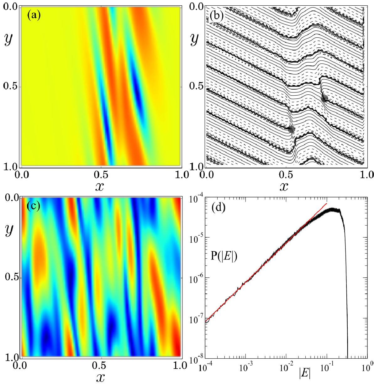
Figure 4: Dynamics of the solution $E$ of the system (5), represented as snapshot in the pseudo space, for the parameter values: $\tau_{1}=10^{2}$, $\tau_{2}=10^{4}$, $\eta_{1}=\eta_{2}=0.1$, $T=10^{2}$, and $J=-0.17$. (a), (b): amplitude and phase of $E$ for $\alpha=2$, showing the occurrence of spiral defects. (c): amplitude of $E$, defects turbulence regime for $\alpha=4$. (d) Statistics of the field amplitude in the case (c); the line is a power-law fit of the tail with exponent $0.98$.

In conclusion, we have discussed a class of systems describing the interplay of the oscillatory instability with multiple, hierarchically long, delayed feedbacks. We have shown that a generalized spatio-temporal representation is able to uncover multiscale features otherwise hidden in the complex temporal dynamics. In the case of two delays, the existence of regimes of FS and DT has been evidenced. By means of a multiple scale analysis, an equivalence is shown to a two-dimensional Complex-Ginzburg Landau equation. The attainment of the long-delay regime have been also analyzed. Finally, we showed how the above phenomena occur in the case study of a semiconductor laser with two external cavity optical feedbacks, a generalization of a well known and studied configuration. As a perspective, our approach can be applied in several experimental setups and in the study of higher-dimensional pattern formations in delay systems, such that the existence and characterization of line defects in the three delays case. Moreover, we expect that this formalism could be generalized for other types of bifurcations as well and applied to the study of specific experimental systems, such as delayed networks like those commonly found in optical communications.

We acknowledge the DFG for financial support in the framework of International Research Training Group 1740 and useful discussions with A. Politi.

I Appendix: Destabilization of the steady state

Prior to deriving the Ginzburg-Landau normal form, it is important to study the destabilization of the steady state $z=0$. The type of the destabilization will give us the key to what kind of normal form is governing the dynamics.

The characteristic equation, which determines the stability of the zero steady state $z=0$ is obtained by linearizing Eq. (1, main text) and substituting $z=e^{\lambda t}$:

$$\lambda-a-be^{-\lambda/\varepsilon}-ce^{-\lambda\kappa/\varepsilon^{2}}=0.$$ (6)

Stability of the steady state is equivalent to that all roots $\lambda$ of (6) have negative real parts. Although the solutions to (6) are not given explicitly, their approximations can be found using the smallness of $\varepsilon$ D’Huys et al. (2013); Heiligenthal et al. (2011); Wolfrum et al. (2010) (largeness of the delays)

$$\lambda=\gamma_{0}+i\omega_{0}+\varepsilon\left(\gamma_{1}+i\omega_{1}\right)+\varepsilon^{2}\left(\gamma_{2}+i\omega_{2}\right),$$ (7)

where $\gamma_{j}$ and $\omega_{j}$ are real. Depending on the leading terms in the real part of this expansion, the system may develop different types of instabilities: if $\gamma_{0}>0$, there appear strong instability induced by the instantaneous term Lepri et al. (1994); Wolfrum and Yanchuk (2006); Yanchuk and Wolfrum (2010); Heiligenthal et al. (2011); Lichtner et al. (2011). If $\gamma_{0}=0$ but $\gamma_{1}>0$, there appears a weak instability by the effect of the $\tau_{1}$-feedback. In this case, the $\tau_{2}$-feedback does not play any role. Hence, in order for the second delay to play the destabilizing role, one needs $\gamma_{0}=\gamma_{1}=0$ and $\gamma_{2}$ becoming positive. By requiring this and substituting (7) into (6), one can arrive to the following conditions for the parameters of the system: $a<0$ and $|b|<|a|$. Moreover, the leading terms in the real part of $\lambda$ can be found explicitly in this case

$$\gamma_{2}(\omega_{0},\phi)=-\frac{1}{2\kappa}\ln\frac{\left(a+|b|\cos\phi\right)^{2}+\left(\omega_{0}+|b|\sin\phi\right)^{2}}{|c|^{2}},$$

where $\phi=-\omega_{1}-\frac{\omega_{0}}{\varepsilon}+\arg(b)$. If the condition $|c|<-a-|b|$ is satisfied, the function $\gamma_{2}$ is negative for all $\omega_{0}$ and $\phi$, implying the stability of the steady state. Otherwise, $\gamma_{2}$ becomes positive and the steady state is unstable for all small enough $\varepsilon$. In this case, a nontrivial dynamics is expected.

The obtained conditions determine when the $\tau_{2}$-feedback destabilize the steady state. Namely, we have $a<0$, $|b|<|a|$, and $P=a+|b|+|c|$, with $P$ as the destabilization parameter. The desired destabilization occurs for positive values of $P$. For our purposes, the destabilization parameter $P$ is chosen as $P=\varepsilon^{2}p=a+|b|+|c|$, where the choice of the smallness factor of $\varepsilon^{2}p$ prevents the unbounded increasing of the number of unstable linear modes (unstable solutions of (6)) with the decreasing of $\varepsilon$ [see more details in Wolfrum and Yanchuk (2006)].

II Appendix: Normal form equation

Here we present a sketch of the formal derivation of the normal form equation (2) from the main text as well as its boundary conditions. System with time delay close to the destabilization has the following perturbative form:

$$z^{\prime}(t)=\left(a+p_{a}\varepsilon^{2}\right)z(t)+\left(Be^{i\phi}+p_{b}\varepsilon^{2}\right)z\left(t-\frac{1}{\varepsilon}\right)+\left(\left(-a-B\right)e^{i\xi}+p_{c}\varepsilon^{2}\right)z\left(t-\frac{\kappa}{\varepsilon^{2}}\right)-dz(t)|z(t)|^{2}$$ (8)

where $a<0,$ $B<-a.$ As follows from the spectrum analysis (previous section), the destabilization takes place at $p_{a}=p_{b}=p_{c}=0$. Our aim is to obtain an equivalent amplitude equations. For this, the multiscale ansatz $z(t)=\varepsilon\left[u_{1}\left(T_{1},T_{2},T_{3},T_{4},\dots\right)+\varepsilon u_{2}\left(\cdots\right)+\varepsilon^{2}u_{3}\left(\cdots\right)+\dots\right],$ $T_{j}=\varepsilon^{j}t$, is substituted in (8) and the obtained expression is expanded in powers of the small parameter $\varepsilon$. Afterward, terms with the same smallness factor $\varepsilon^{j}$ are compared.

In particular, for $\varepsilon^{1}$ we obtain the following solvability conditions

$$u_{1}(T_{1},T_{2},\dots)=e^{i\phi}u_{1}(T_{1}-1,T_{2},\dots)$$

and

$$u_{1}(T_{1},T_{2},\dots)=e^{i\xi}u_{1}(T_{1}-\frac{\kappa}{\varepsilon},T_{2}-\kappa,\dots)=e^{i\left(\xi-\phi\left[\frac{\kappa}{\varepsilon}\right]_{in}\right)}u_{1}(T_{1}-\left\{\frac{\kappa}{\varepsilon}\right\}_{f},T_{2}-\kappa,\dots),$$

where $\left\{\cdot\right\}_{f}$ is the fractional and $\left[\cdot\right]_{in}$ integer part of a number. These conditions will result into the boundary conditions of the normal form equation.

For $\varepsilon^{2}$, we obtain

$$\partial_{T_{1}}u_{1}=-B\partial_{T_{2}}u_{1}+\left(a+B\right)\partial_{T_{3}}u_{1}.$$

This condition connects $\partial_{T_{1}}$ with $\partial_{T_{2}}$ and $\partial_{T_{3}}$ (a kind of transport). This means that the solution depends only on 3 variables:

$$x=T_{1}+\frac{1}{a+B}T_{3};\quad y=T_{2}+\frac{B}{a+B}T_{3};\quad\theta=T_{4}.$$

Hence, instead of $u_{1}$, we introduce new function $\Phi$ as follows

$$u_{1}(T_{1},T_{2},T_{3},T_{4})=\Phi\left(T_{1}+\frac{1}{a+B}T_{3},T_{2}+\frac{B}{a+B}T_{3},T_{4}\right)=:\Phi(x,y,\theta).$$ (9)

Finally, $\varepsilon^{3}$ terms lead to

$$-\left(a+B\right)\partial_{T_{4}}u_{1}=Pu_{1}-\partial_{T_{2}}u_{1}-B\partial_{T_{3}}u_{1}+\frac{1}{2}B\partial_{T_{2}T_{2}}u_{1}-\left(a+B\right)\frac{1}{2}\partial_{T_{3}T_{3}}u_{1}-du_{1}|u_{1}|^{2},$$

where $P=p_{a}+p_{b}e^{-i\phi}+p_{c}e^{-i\xi}$. Rewriting the obtained equation for the new function $\Phi$, we obtain the Ginzburg-Landau equation

$$\left|a+B\right|\partial_{\theta}\Phi=P\Phi+\frac{B}{\left|a+B\right|}\partial_{x}\Phi-\left[1-\frac{B^{2}}{\left|a+B\right|}\right]\partial_{y}\Phi+\frac{1}{2}\frac{1}{\left|a+B\right|}\partial_{xx}\Phi+\frac{B}{\left|a+B\right|}\partial_{xy}\Phi-\frac{1}{2}\frac{aB}{\left|a+B\right|}\partial_{yy}\Phi-d\Phi|\Phi|^{2}$$

(compare Eq. (2) from the main text) equipped with the boundary conditions $\Phi(\theta,x,y)=e^{i\phi}\Phi(\theta,x-1,y)$ and $\Phi(\theta,x,y)=\exp\left[i\left(\xi-\phi\left[\frac{\kappa}{\varepsilon}\right]_{i}\right)\right]\Phi\left(\theta,x-\left\{\frac{\kappa}{\varepsilon}\right\}_{f\mbox{ }},y-\kappa\right)$. The simplest case of the periodic boundary conditions on the domain $\left[0,1\right]^{2}$ arise for $\xi=\varphi=0$ (real parameters $c$ and $b$), $\kappa=1$, and $\left\{\frac{\kappa}{\varepsilon}\right\}_{f\mbox{ }}=0$. The last condition means that the $\tau_{2}/\tau_{1}$ is a large but integer number. Note that the proposed derivation is technically different from the one given in Giacomelli and Politi (1996) for the case of one delay. Just to mention a few, the differences are in the way how boundary conditions are handled and how different timescales appear in the normal form equation. For instance, the timescale $\sim\tau^{3}$ appears for the one-delay case as the temporal variable of the normal form, while here this is just a drifting part of the space coordinates $x$ and $y$.

Figure 5 shows the snapshots of the solutions of the normal form equation corresponding to the defects and turbulence regimes (compare with Figs. 1 and 2 form the main text).

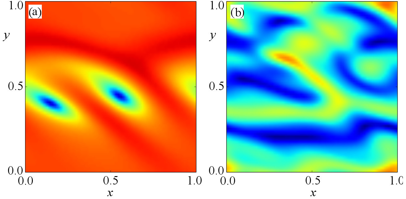
Figure 5: Snapshots for the solutions of the Ginzburg-Landau normal form equation (Eq. (2) in the main text). (a) Spiral defects, parameter values: $p=250,$ $a_{1}=1.11$, $a_{2}=-1.22$, $a_{3}=1.39$, $a_{4}=1.11$, $a_{5}=0.56$, $d=-0.75+i$. (b) Defect turbulence, parameter values are the same except for $d=-0.1+i$. Initial values are random and close to zero.

References

- Li et al. (2011) X. Li, A. B. Cohen, T. E. Murphy, and R. Roy, Optics Lett. 36, 1020 (2011).
- Zamora-Munt et al. (2010) J. Zamora-Munt, C. Masoller, J. Garcia-Ojalvo, and R. Roy, Phys. Rev. Lett. 105, 264101 (2010).
- Giacomelli et al. (2012) G. Giacomelli, F. Marino, M. A. Zaks, and S. Yanchuk, EPL (Europhysics Letters) 99, 58005 (2012).
- Soriano et al. (2013) M. C. Soriano, J. García-Ojalvo, C. R. Mirasso, and I. Fischer, Rev. Mod. Phys. 85, 421 (2013).
- Szalai and Orosz (2013) R. Szalai and G. Orosz, Phys. Rev. E 88, 040902 (2013).
- Izhikevich (2006) E. M. Izhikevich, Neural Computation 18, 245 (2006).
- Appeltant et al. (2011) L. Appeltant, M. C. Soriano, G. Van der Sande, J. Danckaert, S. Massar, J. Dambre, B. Schrauwen, C. R. Mirasso, and I. Fischer, Nature Comm 2 (2011).
- Erneux (2009) T. Erneux, Applied Delay Differential Equations (Springer, 2009).
- Farmer (1982) J. D. Farmer, Physica D 4, 366 (1982).
- Giacomelli et al. (1995) G. Giacomelli, S. Lepri, and A. Politi, Phys. Rev. E 51, 3939 (1995).
- Heiligenthal et al. (2011) S. Heiligenthal, T. Dahms, S. Yanchuk, T. Jüngling, V. Flunkert, I. Kanter, E. Schöll, and W. Kinzel, Phys. Rev. Lett. 107, 234102 (2011).
- D’Huys et al. (2013) O. D’Huys, S. Zeeb, T. Jüngling, S. Heiligenthal, S. Yanchuk, and W. Kinzel, EPL (Europhysics Letters) 103, 10013 (2013).
- Giacomelli and Politi (1996) G. Giacomelli and A. Politi, Phys. Rev. Lett. 76, 2686 (1996).
- Wolfrum and Yanchuk (2006) M. Wolfrum and S. Yanchuk, Phys. Rev. Lett. 96, 220201 (2006).
- Arecchi et al. (1992) F. Arecchi, G. Giacomelli, A. Lapucci, and R. Meucci, Phys. Rev. A 45, 4225 (1992).
- Giacomelli et al. (1994) G. Giacomelli, R. Meucci, A. Politi, and F. T. Arecchi, Phys. Rev. Lett. 73, 1099 (1994).
- Larger et al. (2013) L. Larger, B. Penkovsky, and Y. Maistrenko, Phys. Rev. Lett. 111, 054103 (2013).
- Chaté and Manneville (1996) H. Chaté and P. Manneville, Physica A: Statistical Mechanics and its Applications 224, 348 (1996).
- Aranson and Kramer (2002) I. Aranson and L. Kramer, Rev. Mod. Phys. 74, 99 (2002).
- Deissler and Kaneko (1987) R. J. Deissler and K. Kaneko, Phys. Lett. A 119, 397 (1987).
- Lang and Kobayashi (1980) R. Lang and K. Kobayashi, IEEE J. Quantum Electron. 16, 347 (1980).
- Barland et al. (2005) S. Barland, P. Spinicelli, G. Giacomelli, and F. Marin, IEEE J. Quantum Electron. 41, 1235 (2005).
- Wolfrum et al. (2010) M. Wolfrum, S. Yanchuk, P. Hövel, and E. Schöll, Eur. Phys. J. Special Topics 191, 91 (2010).
- Lepri et al. (1994) S. Lepri, G. Giacomelli, A. Politi, and F. T. Arecchi, Physica D 70, 235 (1994).
- Yanchuk and Wolfrum (2010) S. Yanchuk and M. Wolfrum, SIAM J Appl Dyn Syst 9, 519 (2010).
- Lichtner et al. (2011) M. Lichtner, M. Wolfrum, and S. Yanchuk, SIAM J. Math. Anal. 43, 788 (2011).