Guiding-center Hall viscosity and intrinsic dipole moment
along edges of incompressible fractional quantum Hall fluids

Abstract

The discontinuity of guiding-center Hall viscosity (a bulk property) at edges of incompressible quantum Hall fluids is associated with the presence of an intrinsic electric dipole moment on the edge. If there is a gradient of drift velocity due to a non-uniform electric field, the discontinuity in the induced stress is exactly balanced by the electric force on the dipole. The total Hall viscosity has two distinct contributions: a “trivial” contribution associated with the geometry of the Landau orbits, and a non-trivial contribution associated with guiding-center correlations. We describe a relation between the guiding-center edge-dipole moment and “momentum polarization”, which relates the guiding-center part of the bulk Hall viscosity to the “orbital entanglement spectrum(OES)”. We observe that using the computationally-more-onerous “real-space entanglement spectrum (RES)” just adds the trivial Landau-orbit contribution to the guiding-center part. This shows that all the non-trivial information is completely contained in the OES, which also exposes a fundamental topological quantity $\gamma$ = $\tilde{c}-\nu$, the difference between the “chiral stress-energy anomaly” (or signed conformal anomaly) and the chiral charge anomaly. This quantity characterizes correlated fractional quantum Hall fluids, and vanishes in uncorrelated integer quantum Hall fluids.

I Introduction

During the period of three decades since the first observationTsui et al. (1982), incompressible fractional quantum Hall (FQH) states have been shown to possess many intriguing properties, and one of these is the “Hall viscosity”Avron et al. (1995); Read (2009); Read and Rezayi (2011); Haldane (2009). The total Hall viscosity tensor $\eta^{\prime}_{H}\,{}^{ab}_{cd}$ of an incompressible FQH state is a sum of two parts of different origins,

$$\eta_{H}^{\prime}\,{}^{ab}_{cd}=\tilde{\eta}_{H}\,^{ab}{}_{cd}+\eta_{H}\,^{ab}{}_{cd}.$$

The former, “Landau-orbit Hall viscosity” $\tilde{\eta}_{H}\,^{ab}{}_{cd}$, is the response to the variation of the shape of the Landau-orbit(i.e. cyclotron motion), and the latter, “guiding-center Hall viscosity” $\eta_{H}\,^{ab}{}_{cd}$, is the response to the variation of the shape of the correlation hole. Each of these two shapes can be parameterized by a 2$\times$2 spatial metricHaldane (2011). The metric associated with the Landau-orbit shape is called “Landau-orbit metric” and the one associated with the correlation hole shape is called “guiding-center metric”. The generalization by HaldaneHaldane (2011) to dynamical variation of the guiding-center metric led to a new research interest for the geometric description of incompressible FQH statesHoyos and Son (2012); Maciejko et al. (2013).

There have been attempts to link the Hall viscosity with other physical observable such as the Hall conductivity Hoyos and Son (2012); Bradlyn et al. (2012). The basic assumption of those calculations is Galilean invariance. However, an incompressible FQH state is a topological phase for which such assumption should not be essential. In this report, we relate the guiding-center Hall viscosity, i.e. the part of the Hall viscosity due to the guiding-center degrees of freedom, with the intrinsic dipole moment per unit length along the edge of incompressible FQH statesHaldane (2009). Though we will do the computation for a straight edge, the result is applicable to the edge of an arbitrary shape because the relationship derives from the local force balance at a point on the edge.

Another aim of this report is to show that we can calculate the intrinsic dipole moment from the “orbital entanglement spectrum” (OES)Li and Haldane (2008). Therefore, OES contains enough information to determine the guiding-center Hall viscosity. The intrinsic dipole moment is essentially the non-vanishing mean momentum due to the entanglement with the other half of the whole system (also called “momentum polarization”). For a finite length $L$ of the edge, there is a correction of order $\mathcal{O}(L^{0})$. This correction is composed of two parts, “topological spin”Zaletel et al. (2013); Tu et al. (2013) and a new topological quantity $\gamma=\tilde{c}-\nu$ which is the difference between signed conformal anomaly $\tilde{c}$ and chiral charge anomaly $\nu$ of the underlying edge theoryWen (1991). We also elucidate the origins of the topological spin and the fractional charge by showing that they originate from different cuts relative to the “root occupation pattern”Bernevig and Haldane (2008).

The last goal of this report is to show that the computation of Hall viscosity with the so-called “real-space entanglement spectrum” (RES)Dubail et al. (2012); Zaletel et al. (2013) merely adds “Landau-orbit Hall viscosity” which is a rather trivial part of the Hall viscosity due to the cyclotron motion. For a finite length $L$, RES also adds the chiral anomaly $\nu$ to the $\mathcal{O}(L^{0})$ correction, and therefore obscures the existence of the new topological quantity $\gamma$. We are led to claim that all the essential information of FQH states are contained in OES.

First of all, let’s clarify what we mean by the intrinsic dipole moment. Consider electrons on a cylinder through whose surface an uniform magnetic field $B$ passes. We confine the electrons by an external electric potential $V(y)$ that depends on $y$, one of the two spatial coordinates, $x$ and $y$. Then, single-particle states $|\phi_{m}\rangle$ are labeled by guiding-centers $y_{m}=2\pi m\ell_{B}^{2}/L$, $m\in\mathbb{Z}+\textstyle{\frac{1}{2}}$ ($\ell_{B}^{2}=\hbar/eB$). Given a many-particle state $|\Psi\rangle$, we can calculate its occupation-number profile which is the set of the expectation values of occupation-number operators $n_{m}$ for each index $m$. For instance, consider an IQH state in the first Landau level, $|\Psi_{1}\rangle$, filling the upper-half plane with a “Fermi momentum” at $y=0$ (See Fig.1(a)). Then, its occupation profile is $\{\dots,n_{-3/2},n_{-1/2},n_{1/2},n_{3/2},\dots\}=\{\dots,0,0,\nu,\nu,\dots\}$ where the filling factor $\nu=1$. In the continuum limit $L\rightarrow\infty$, the occupation profile for this uncorrelated state is a step function in $y$ : $n(y)=\nu\,\theta(y)$.

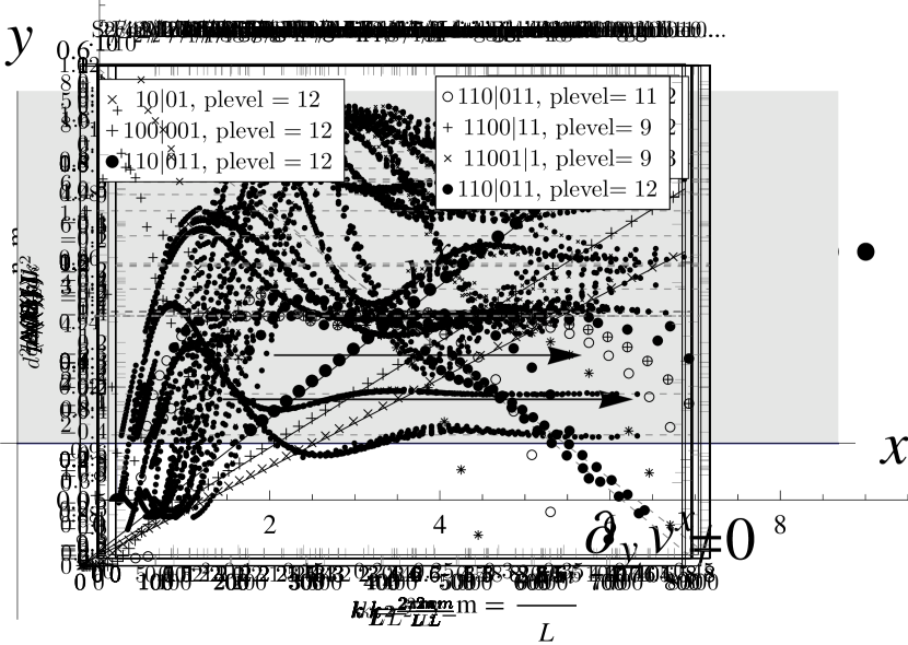
(a) A straight edge

(b) An arbitrary edge

Figure 1: The gray area represents the Hall fluid. In general, the drift velocity depends on the distance from the edge. Each edge follows an equipotential line.

Now, let’s consider as an example of a correlated state, the Laughlin $\nu=\textstyle{\frac{1}{3}}$ stateLaughlin (1983), $|\Psi_{1/3}\rangle$. As before, suppose the Fermi momentum is at $y=0$ (when the circumference $L$ is finite, it is not obvious where the Fermi momentum is. This will be clarified later, Sec.III.2). For a given $L$, we can obtain a occupation profile. For $L=15\ell_{B}$, we have the occupation profile in Fig.2. Unlike the uncorrelated state $|\Psi_{1}\rangle$, the occupation profile of the correlated state $|\Psi_{1/3}\rangle$ deviates from the filling factor $\nu=\textstyle{\frac{1}{3}}$ near the edge. In the continuum limit, the occupation profile becomes $n(y)\propto y^{(\nu^{-1}-1)}$ as predicted by chiral boson theoryWen (1991) (cf. Sec.III.3). We see that the correlation among the electrons develops an extra “intrinsic dipole moment” at the edge by “pulling them inward” (this corresponds to the fact that FQH model wavefunctions are spanned by states obtainable by “squeezing” the “root state”Bernevig and Haldane (2008), See Sec.III.1).

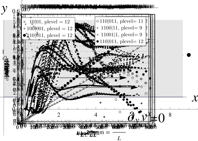
Figure 2: Occupation profile ($\bullet$) for Laughlin $\nu=1/3$ state and the uniform occupation profile $\bar{n}_{m}=\nu$ ($\circ$) on a cylinder with circumference $L=15$ ($\ell_{B}=1$).

Because an incompressible FQH state is a topological phase, the straightness of the edge should not be essential. Therefore, we consider an edge of an arbitrary shape as in Fig.1(b) on a flat 2D plane. We denote the line element along the edge by $dL^{a}$. We relate the intrinsic dipole moment $dp^{a}$ per a line element $dL^{a}$ by introducing a dimensionless symmetric 2-tensor $Q^{ab}$,

$$dp^{a}=-e\,Q^{ab}\epsilon_{bc}dL^{c}.$$

The electric charge $-e$ is negative, and $\epsilon_{ab}=\epsilon^{ab}$ is the Levi-Civita anti-symmetric tensor, $\epsilon_{xy}=-\epsilon_{yx}=1$. Throughout this report, we distinguish covariance and contravariance of indices, and we use the Einstein summation convention. In general, the electric field which derives from the Coulomb interaction and the confining potential is not constant but depends on the distance from the edge. The gradient of the electric field coupled with the intrinsic dipole moment results in an electric force,

$$dF_{\text{el},a}=dp^{b}\partial_{a}E_{b}.$$

If the edge is to be stable, this electric force should be balanced. What should this counter-balancing force be? The counter-balancing force against the electric force on the intrinsic dipole comes from the guiding-center Hall viscosity. Here, we review the physical argumentHaldane (2009), and then we will provide two kinds of numerical proofs, first utilizing the exact model wavefunctions in Sec.III and secondly utilizing the orbital entanglement spectra in Sec.IV.1.

Firstly, we note that pressure is absent. An incompressible FQH state is a topological quantum phase. In the bulk, all excitations are separated by an energy gap, and its low-energy effective description is the Chern-Simons LagrangianZhang et al. (1989) with a vanishing Hamiltonian. Because the incompressible state has no phonons to mediate the effect of external force, the bulk pressure vanishes entirelyHaldane (2009).

We should take into account only the guiding-center part of the total Hall viscosity because the “trivial” Landau-orbit Hall viscosity $\tilde{\eta}_{H}\,^{ab}{}_{cd}$ is present whether or not the electrons are correlated (this part of the Hall viscosity will be discussed together with RES in Sec.IV.3). When the electrons develop correlations among themselves, there arises the additional non-trivial guiding-center Hall viscosity $\eta_{H}\,^{ab}{}_{cd}$, concurrently with the intrinsic dipole moment.

The non-uniform electric field near the edge results in a non-vanishing gradient of the drift velocity $v^{a}=\epsilon^{ab}E_{b}/B$. Then, the edge experiences a dissipationless stress $\sigma_{a}^{b}$ due to the guiding-center Hall viscosity proportional to the gradient of the drift velocity,

$$\sigma^{a}_{b}=-\eta_{H}\,^{ac}{}_{bd}\,\partial_{c}v^{d}=-\eta_{H}^{aecf}\epsilon_{eb}\epsilon_{fd}\,\partial_{c}v^{d}.$$

where in the second equality, we raised the two lower indices of $\eta_{H}\,^{ac}{}_{bd}$ using Levi-Civita tensors. Note that $\eta_{H}^{abcd}$ is anti-symmetric under the exchange of the two pairs of indices $(ab)\leftrightarrow(cd)$, and symmetric under the exchange of two indices $a\leftrightarrow b$ or $c\leftrightarrow d$ (cf. Sec.II.2). Such 4-tensor can be expanded in terms of a symmetric 2-tensor $\eta_{H}^{ab}$,

$$\eta_{H}^{abcd} =\textstyle{\frac{1}{2}}(\epsilon^{ac}\eta_{H}^{bd}+\epsilon^{ad}\eta_{H}^{bc}+a\leftrightarrow b).$$

With this expansion, the expression for the stress tensor becomes

$$\sigma_{b}^{a}=\textstyle{\frac{1}{2}}B^{-1}(\epsilon^{ac}\epsilon_{eb}\eta_{H}^{ef}+\delta^{c}_{b}\eta_{H}^{af}+c\leftrightarrow f)\,\partial_{c}E_{f}$$

From the stress, we find the dissipationless viscous force $dF_{\text{visc},a}$ on a line element $dL^{a}$,Landau and Lifshitz (1986)

$$dF_{\text{visc},a}=\sigma_{a}^{b}\epsilon_{bc}dL^{c}.$$

We make two physical assumptions to reduce the viscous force equation further. The first assumption is that the magnetic field is static so that the Maxwell’s equation gives $\epsilon^{ab}\partial_{a}E_{b}=0$. This implies the 2-tensor $\partial_{a}E_{b}$ is symmetric under the exchange of the indices, $a\leftrightarrow b$. The second assumption is that the line element $dL^{a}$ of the edge is directed along the equipotential line so that $E_{a}dL^{a}=0$. From these two assumptions, the viscous force reduces to

$$dF_{\text{visc},a}=(B^{-1}\eta^{bc}_{H}\epsilon_{cd}dL^{d})\partial_{a}E_{b}.$$

Then, from the requirement that the net force on the line element vanishes, $dF_{\text{el},a}+dF_{\text{visc},a}=0$, we obtain the relationship between the intrinsic dipole moment tensor $Q^{ab}$ and the guiding-center Hall viscosity 2-tensor $\eta_{H}^{ab}$,

$$\eta_{H}^{ab}=eBQ^{ab}.$$

Thus, if we know the guiding-center Hall viscosity tensor $\eta_{H}^{ab}$, we also know the intrinsic dipole moment $dp^{a}$ along the static equipotential edge,

$$dp^{a}=-B^{-1}\eta^{ab}_{H}\epsilon_{bc}dL^{c}.$$ (1)

This relationship (1) between the intrinsic dipole moment and the guiding-center Hall viscosity tensor was derived from a local balance of forces. Therefore, we expect the relationship to hold for an edge of any smooth arbitrary shape reflecting the topological nature of an incompressible FQH state.

To give a specific example, consider the situation depicted in Fig.1(a) for which $\partial_{y}v^{x}$ is the only non-vanishing component of the velocity gradient. Then, the stress expression reduces to

$$\sigma^{y}_{y}=-\eta^{yy}_{H}\frac{\partial_{y}E_{y}}{B}.$$

The viscous force per a line element $dL^{x}$ on the edge is given by

$$dF_{\text{visc},y}=\eta^{yy}_{H}\frac{\partial_{y}E_{y}}{B}dL^{x}.$$

The electric force on the dipole for this situation is

$$dF_{\text{el},y}=-e\,Q^{yy}dL^{x}\partial_{y}E_{y}.$$

Vanishing of the net force gives us,

$$\frac{dp^{y}}{dL^{x}}=\frac{\eta^{yy}_{H}}{B}.$$ (2)

The left-hand side of (2) can be numerically calculated from occupation profiles (for instance, Fig.2). This will be done in Sec.III and Sec.IV. The right-hand side of (2) can be analytically calculated as the expectation value of the “area-preserving deformation generators”. This calculation is described in Sec.II.

II Theoretical Background

In this section, we describe the distinct physical origins of the Landau orbit metric and the guiding-center metric. The Landau-orbit Hall viscosity and the guiding-center Hall viscosity are derived as the adiabatic responses to the variation of the Landau orbit metric and the guiding-center metric respectively, and as the expectation values of area-preserving deformation generators. We calculate these quantities for the model LaughlinLaughlin (1983) and Moore-ReadMoore and Read (1991) states.

II.1 Landau-orbit metric and guiding-center metric

Consider $N$ electrons with charge $-e<0$ living on a 2D plane subject to a normal magnetic field strength $\bm{B}=B\hat{z}$, $B>0$. The $i$-th electron on the 2D plane has four degrees of freedom, its coordinate $\bm{r}_{i}$ and its dynamical momentum $\bm{\pi}_{i}=\bm{p}_{i}+e\bm{A}(\bm{r}_{i})$. Note that $i,j,\dots$ are indices for electrons, and $a,b,\dots$ are indices for the spatial coordinates. The coordinate operator can be decomposed into two operators

$$\bm{r}_{i}=\bm{R}_{i}+\tilde{\bm{R}_{i}},$$ (3)

where the first operator $\bm{R}_{i}$ is the “guiding-center of the electron, and the second operator $\tilde{\bm{R}_{i}}$ is the “Landau-orbit radii”. The Landau-orbit radii is defined in terms of the dynamical momenta: $\tilde{R}^{a}_{i}=\epsilon^{ab}\pi_{b}/eB$. These operators have the following commutation relations,

$$[\tilde{R}_{i}^{a},\tilde{R}_{j}^{b}] =-i\epsilon^{ab}\delta_{ij}\ell_{B}^{2}$$ (4a)

$$[R_{i}^{a},R_{j}^{b}] =i\epsilon^{ab}\delta_{ij}\ell_{B}^{2}$$ (4b)

$$[\tilde{R}_{i}^{a},R_{j}^{b}] =0,$$ (4c)

where $\ell_{B}^{2}=\hbar/eB$. This decoupling between $\bm{R}_{i}$ and $\tilde{\bm{R}}_{i}$ is completely independent of the choice of a gauge.

Out of these operators, we can form area-preserving deformation (APD) generatorsHaldane (2011)

$$\Lambda^{ab} =\textstyle{\sum_{i}}\Lambda^{ab}_{i}=\textstyle{\frac{1}{4\ell_{B}^{2}}}\sum_{i}\{R_{i}^{a},R_{i}^{b}\}$$ (5a)

$$\tilde{\Lambda}^{ab} =\textstyle{\sum_{i}}\tilde{\Lambda}^{ab}_{i}=\textstyle{\frac{1}{4\ell_{B}^{2}}}\sum_{i}\{\tilde{R}_{i}^{a},\tilde{R}_{i}^{b}\},$$ (5b)

where $\{\,,\,\}$ is an anti-commutation. These satisfy the commutation relations of $\mathfrak{sl}(2,\mathbb{R})$

$$[\Lambda^{ab},\Lambda^{cd}] =+\textstyle{\frac{i}{2}}(\epsilon^{ac}\Lambda^{bd}+\epsilon^{ad}\Lambda^{bc}+a\leftrightarrow b)$$ (6a)

$$[\tilde{\Lambda}^{ab},\tilde{\Lambda}^{cd}] =-\textstyle{\frac{i}{2}}(\epsilon^{ac}\tilde{\Lambda}^{bd}+\epsilon^{ad}\tilde{\Lambda}^{bc}+a\leftrightarrow b).$$ (6b)

The interacting electrons are described by the following Hamiltonian $H$ which is a sum of a single-particle energy $H_{0}$ and the interaction $V$,

$$H =H_{0}+V$$

$$V =\textstyle{\frac{1}{2}}\sum_{i\neq j}V(\bm{r}_{i}-\bm{r}_{j};\varepsilon).$$ (7)

Note that the Coulomb interaction $V$ also depends on the permittivity tensor $\varepsilon_{ab}$. The most general single-particle energy is

$$H_{0}=\textstyle{\sum_{i}}h(\tilde{\bm{R}}_{i}),$$

where $h(\bm{r})$ is a function of $\bm{r}$ whose constant contours are non-overlapping and closed. The most general form of the single-particle energy is technically intractable, so we take a model single-particle energy parameterized by a unimodular symmetric positive-definite 2-tensors $\tilde{g}_{ab}$ which we call the “Landau-orbit metric”,

$$H_{0}=\textstyle{\sum_{i}}h(\tilde{g}_{ab}\tilde{R}_{i}^{a}\tilde{R}_{i}^{b}),$$ (8)

where $h(r)$ is a monotonically increasing function of $r$. This form includes, for instance, the following two examples which break Galilean invariance,

$$H_{0} =\textstyle{\sum_{i}}(\tilde{g}_{ab}\Lambda_{i}^{ab})^{k+1},\quad k\in\mathbb{N}$$

$$H_{0} =\textstyle{\sum_{i}}\sqrt{1+\tilde{g}_{ab}\Lambda_{i}^{ab}},$$

The second example is the massive Dirac Hamiltonian of a charged particle subject to a normal magnetic field.

If the system is Galilean invariant, the Landau-orbit metric $\tilde{g}_{ab}$ is determined by the effective mass tensor $(m^{-1})^{ab}$,

$$H_{0} =\textstyle{\frac{1}{2}}(m^{-1})^{ab}\sum_{i}\pi_{i,a}\pi_{i,b}$$

$$=\textstyle{\frac{1}{2}}\hbar\omega_{c}\,\tilde{L}(\tilde{g})$$

$$\tilde{L}(\tilde{g}) =\textstyle{\sum_{i}}\tilde{L}_{i}(\tilde{g})=\textstyle{\sum_{i}}\tilde{g}_{ab}\tilde{\Lambda}_{i}^{ab},$$

where the cyclotron frequency is $\omega_{c}=eB/|m|$ and $|m|=\det m$. We also defined the rotation generator of Landau-orbit radii, $\tilde{L}(\tilde{g})$. The eigenvalues of $\tilde{L}_{i}(\tilde{g})$ are $\tilde{s}_{n}=n+\textstyle{\frac{1}{2}},\,n\in\mathbb{Z}_{+}$, and we call $\tilde{s}_{n}$ the “Landau-orbit spin”.

For the single-particle energy (8), we can label the Landau level with the non-negative integer $n$ from the eigenvalue of $\tilde{L}_{i}(\tilde{g})$. Note that the system without Galilean invariance has an unequal energy gap between neighboring Landau levels.

In the strong magnetic field strength limit where Landau level mixing is not allowed, the Landau-orbit and guiding-center degrees of freedom decouple. Then, the many-particle ground state $|\Psi\rangle$ of the Hamiltonian $H$ in the $n$-th Landau level can be decomposed as a tensor product,

$$|\Psi\rangle=(\textstyle{\prod_{i}}|\psi_{i,n}\rangle_{L})\otimes|\Psi(g)\rangle_{G}.$$ (9)

The vectors with the subscript $L$ (for Landau-orbit) can be acted on only by the Landau-orbit operators $\tilde{\bm{R}}_{i}$ and the vectors with the subscript $G$ (for guiding-center) can be acted on only by the guiding-center operators $\bm{R}_{i}$. The vector $|\psi_{i,n}\rangle_{L}$ is the $n$-th eigenstate of $\tilde{L}_{i}(\tilde{g})$.

We now discuss how the guiding-center part $|\Psi(g)\rangle_{G}$ is determined. Since the Landau-orbit part of $|\Psi\rangle$ is fixed, the interaction $V$ may be projected into the $n$-th Landau level,

$$\Pi_{n}V\Pi_{n}=\frac{1}{2N_{\Phi}}\sum_{\bm{q}}V(\bm{q};\varepsilon)f_{n}(\bm{q})^{2}\rho(\bm{q})\rho(-\bm{q}),$$ (10)

where $\Pi_{n}$ is the projection operator into the $n$-th Landau level, $N_{\Phi}$ is the total number of flux quanta penetrating the QH fluid, $V(\bm{q};\varepsilon)$ is the Fourier-transformation of $V(\bm{r};\varepsilon)$. We define the “Landau-orbit form factor” $f_{n}(\bm{q})$ and the guiding-center density operator $\rho(\bm{q})$ as follows. Consider the Fourier-transformation of the density operator $\rho_{0}(\bm{r})$,

$$\rho_{0}(\bm{q})=\textstyle{\sum_{i}}e^{i\bm{q}\cdot\bm{r}_{i}}.$$

The density operator $\rho_{0}(\bm{q})$ is projected into the $n$-th Landau level by sandwiching the operator with the vector $\textstyle{\prod_{i}}|\psi_{i,n}\rangle_{L}$, and this produces the projected density operator $\rho_{n}(\bm{q})$ as a product of the form factor and the guiding-center density operator,

$$\rho_{n}(\bm{q}) =f_{n}(\bm{q})\rho(\bm{q})$$ (11a)

$$f_{n}(\bm{q}) =\langle\psi_{i,n}|e^{i\bm{q}\cdot\tilde{\bm{R}}_{i}}|\psi_{i,n}\rangle_{L}$$ (11b)

$$\rho(\bm{q}) =\textstyle{\sum_{i}}e^{i\bm{q}\cdot\bm{R}_{i}}.$$ (11c)

If the single-particle energy is of the form (8), the Landau-orbit form factor becomes

$$f_{n}(\bm{q})=L_{n}\left(\textstyle{\frac{1}{2}}|\bm{q}|_{\tilde{g}}^{2}\right)\,e^{-|\bm{q}|_{\tilde{g}}^{2}/4}$$ (12)

where $L_{n}$ is a Laguerre polynomial of degree $n$, and the Landau-orbit metric norm is defined as $|\bm{q}|_{\tilde{g}}^{2}=\tilde{g}^{ab}q_{a}q_{b}\ell_{B}^{2}$ ($\tilde{g}^{ac}\tilde{g}_{cb}=\delta^{a}_{b}$). We can make an alternative definition of the Landau-orbit metric in terms of the Landau-orbit form factor,

$$\tilde{g}^{ab}=\tilde{s}_{n}^{-1}\ell_{B}^{-2}\partial_{q_{a}}\partial_{q_{b}}f_{n}(\bm{q})|_{\bm{q}=\bm{0}}.$$ (13)

This definition gives us the interpretation of the Landau-orbit metric as the parameter which determines the shape of the Landau-orbit.

One can re-write the projected interaction (10) into a more fundamental expansion known as Haldane pseudo-potential Haldane (1983),

$$\Pi_{n}V\Pi_{n} =\sum_{m=0}^{\infty}V_{m}(g,n,\varepsilon)P_{m}(g)$$ (14a)

$$V_{m}(g,n,\varepsilon) =\frac{1}{2N_{\phi}}\sum_{\bm{q}}V(\bm{q};\varepsilon)f_{n}(\bm{q})^{2}L_{m}(|\bm{q}|_{g}^{2})e^{-|\bm{q}|_{g}^{2}}$$ (14b)

$$P_{m}(g) =\frac{1}{N_{\phi}}\sum_{\bm{q}}L_{m}(|\bm{q}|_{g}^{2})e^{-|\bm{q}|_{g}^{2}/2}\rho(\bm{q})\rho(-\bm{q}).$$ (14c)

Here, we introduced a positive-definite symmetric 2-tensor $g_{ab}$ which we call the “guiding-center metric” through the norm $|\bm{q}|_{g}=g^{ab}q_{a}q_{b}\ell_{B}^{2}$ ($g^{ac}g_{cb}=\delta^{a}_{b}$). $P_{m}(g)$ is a projection operator: to understand the action of $P_{m}(g)$, we define the “relative guiding-center rotation generator”,

$$L_{ij}(g)=\textstyle{\frac{1}{8\ell_{B}^{2}}}g_{ab}\{R^{a}_{i}-R^{a}_{j},R^{b}_{i}-R^{b}_{j}\}.$$ (15)

This operator has a spectrum, “relative guiding-center angular momentum” $\{m+\textstyle{\frac{1}{2}}:m\in\mathbb{Z}_{+}\}$. $P_{m}(g)$ has non-vanishing matrix elements for states with a pair of particles with relative guiding-center angular momentum $m+\textstyle{\frac{1}{2}}$.

Instead of using the full expansion as given in (14a), we can form a model interaction,

$$V_{\text{model}}(g)=\sum_{m=0}^{q-1}V_{m}P_{m}(g),$$ (16)

where $V_{m}$ are positive reals and $q$ is some positive integer. The full expansion (14a) does not depend on a particular choice of $g_{ab}$. However, the model interaction does depend on $g_{ab}$. The $\nu=\textstyle{\frac{1}{q}}$ “Laughlin state” is an exact zero energy state of the model interaction ($V_{\text{model}}(g)|\Psi(g)\rangle_{G}=0$). The Laughlin wavefunction is a particular member ($g_{ab}=\tilde{g}_{ab}$) of the family of Laughlin states parameterized by $g_{ab}$ in the Galilean invariant systemHaldane (2011). If the original projected interaction (10) contains the permittivity tensor $\varepsilon_{ab}$ and the Landau-orbit metric $\tilde{g}_{ab}$ that are not related by multiplying a constant, then there is no reason to prefer the isotropic state with $g_{ab}=\tilde{g}_{ab}$.

Therefore, we see that the particular form of the model interaction (i.e. the set of numbers $\{V_{m}\}$) determines the correlation among particles; it tells us what relative guiding-center momenta are energetically unfavorable. Meanwhile, the guiding-center metric determines the shape of the correlation hole.

Given the family of states $\{|\Psi(g)\rangle_{G}:g_{ab}\}$ which minimize $V_{\text{model}}(g)$ and are parameterized by $g_{ab}$, the equilibrium guiding-center metric is finally determined by minimizing the correlation energy,

$$E_{G}(g)=\langle\Psi(g)|\Pi_{n}V\Pi_{n}|\Psi(g)\rangle_{G}.$$ (17)

Note that the guiding-center metric describes an emergent geometry of the correlated electrons while Landau-orbit metric directly comes from the Landau-orbit form factor. The guiding-center metric may vary on the length scale much larger than $\ell_{B}$. Furthermore, it was proposed by HaldaneHaldane (2009) to be a dynamical field that describes the gapped collective mode of the incompressible FQH fluid.

II.2 Hall viscosity

In the last section, we described the definition of the equilibrium values of the Landau-orbit metric and the guiding-center metric. Here, we want to deform the metrics preserving their determinants, and find the Hall viscosities as the response of the incompressible FQH state without assuming Galilean and rotation invariances.

The APD generators preserve the determinant of the metric $g_{ab}$ and $\tilde{g}_{ab}$. To see this (let’s focus on guiding-centers first), define the unitary operator $U(\alpha)$ parameterized by a real symmetric 2-tensor $\alpha_{ab}$,

$$U(\alpha)=\exp i\alpha_{ab}\Lambda^{ab}.$$ (18)

Then, this unitary operator deforms the metric $g_{ab}$ into $g_{ab}^{\prime}$ by group conjugation but leaves the determinant unchanged,

$$L_{ij}(g^{\prime})=U(\alpha)^{\dagger}L_{ij}(g)U(\alpha),\quad\det g^{\prime}=\det g.$$

If $\alpha_{ab}$ is infinitesimal, then the variation in the metric is

$$\delta g_{ab}=-g_{ac}\epsilon^{cd}\alpha_{db}+a\leftrightarrow b.$$ (19)

Suppose that we have an incompressible FQH state $|\Psi\rangle$ of the form (9) whose guiding-center metric minimizes the correlation energy (17). Then, we can define a deformed state

$$|\Psi(\alpha)\rangle=U(\alpha)|\Psi\rangle.$$

We can find the generalized force by the adiabatic response associated with the variation $\alpha_{ab}$,

$$F^{ab}=-\left.\frac{\partial E_{G}(g)}{\partial\alpha_{ab}}\right|_{\alpha=0}+\Gamma^{abcd}\dot{\alpha}_{cd}.$$

The first term vanishes because the correlation energy is minimized for the equilibrium guiding-center metric $g_{ab}$, and the second term is

$$\Gamma^{abcd} =-\hbar\,\text{Im}\langle\partial_{\alpha_{ab}}\Psi(\alpha)|\partial_{\alpha_{cd}}\Psi(\alpha)\rangle|_{\alpha=0}$$

$$=-i\hbar\,\langle\Psi|[\Lambda^{ab},\Lambda^{cd}]|\Psi\rangle.$$

Dividing by the area $A$ occupied by the QH fluid, we find a 4-tensor $\eta_{H}^{abcd}$ which we identify as the guiding-center Hall viscosity tensor with raised indices,

$$\eta^{abcd}_{H}=-\frac{1}{A}\Gamma^{abcd}=\frac{\hbar}{2\pi\ell_{B}^{2}}\frac{i}{N_{\Phi}}\langle\Psi|[\Lambda^{ab},\Lambda^{cd}]|\Psi\rangle.$$ (20)

In the active transformation, the deformation of the metric corresponds to the following mapping of $\bm{R}_{i}$,

$$R_{i}^{a}\rightarrow \quad U(\alpha)^{\dagger}R_{i}^{a}U(\alpha)$$

$$=R_{i}^{a}-i\alpha_{bc}[\Lambda^{bc},R_{i}^{a}]+\mathcal{O}(\alpha^{2})$$

$$=R_{i}^{a}+\epsilon^{ab}\alpha_{bc}R_{i}^{c}.$$

Thus, we identify $\epsilon^{ac}\alpha_{cb}$ as the analog of the derivative of the displacement vector $\partial_{b}u^{a}$ in the classical elasticity theoryLandau and Lifshitz (1986). Then, the guiding-Hall viscosity tensor is

$$\eta_{H}\,^{ac}{}_{bd}=\eta_{H}^{aecf}\epsilon_{eb}\epsilon_{fd}.$$ (21)

We can use the commutation relations of the guiding-center APD generators to expand the 4-tensor $\eta_{H}^{abcd}$ in terms of a symmetric 2-tensor $\eta_{H}^{ab}$,

$$\eta_{H}^{abcd} =\textstyle{\frac{1}{2}}(\epsilon^{ac}\eta_{H}^{bd}+\epsilon^{ad}\eta_{H}^{bc}+a\leftrightarrow b)$$ (22a)

$$\eta_{H}^{ab} =-\frac{\hbar}{2\pi\ell_{B}^{2}}\frac{1}{N_{\Phi}}\langle\Psi|\Lambda^{ab}|\Psi\rangle$$ (22b)

The quantity $\langle\Psi|\Lambda^{ab}|\Psi\rangle$ contains both super-extensive ($\propto N^{2}$) and extensive ($\propto N$) terms. The former contribution comes from the uniform background number-density $\nu/2\pi\ell_{B}^{2}$ ($\nu=N/N_{\Phi}$). This super-extensive term should be subtracted so that the guiding-center Hall viscosity is regularized. The extensive term does not vanish only if the electrons develop correlation.

Now, consider the Landau-orbit degree of freedom. After replacing $\Lambda^{ab}$ with $\tilde{\Lambda}^{ab}$ and $L_{ij}(g)$ with $\tilde{L}(\tilde{g})$, the same argument works. The Landau-orbit Hall viscosity tensor is

$$\tilde{\eta}_{H}\,^{ac}{}_{bd} =\tilde{\eta}_{H}^{aecf}\epsilon_{eb}\epsilon_{fd}$$ (23a)

$$\tilde{\eta}_{H}^{abcd} =\textstyle{\frac{1}{2}}(\epsilon^{ac}\tilde{\eta}_{H}^{bd}+\epsilon^{ad}\tilde{\eta}_{H}^{bc}+a\leftrightarrow b)$$ (23b)

$$\tilde{\eta}_{H}^{ab} =\frac{\hbar}{2\pi\ell_{B}^{2}}\frac{1}{N_{\Phi}}\langle\Psi|\tilde{\Lambda}^{ab}|\Psi\rangle$$ (23c)

The Landau-orbit Hall viscosity does not need regularization. The sign difference between (22b) and (23c) originates from the commutation relations of Landau-orbit and guiding center APD generators, cf.(6). This Landau-orbit Hall viscosity exists whether or not the electrons are correlated. If the single-particle energy is of the form (8), then the Landu-orbit Hall viscosity tensor can be expressed in terms of Landau-orbit spin,

$$\tilde{\eta}_{H}^{ab}=\frac{\hbar}{2\pi\ell_{B}^{2}}\nu\tilde{s}_{n}\tilde{g}^{ab}$$ (24)

This is the Hall viscosity first discussed by Avron, Seiler and Zograf in the Galilean invariant system.Avron et al. (1995)

II.3 Guiding-center spin

In the last section, we derived the two kinds of Hall viscosity without assuming Galilean and rotational symmetry. Furthermore, there was no assumption about the shape of the QH fluid (it could take any shape as in Fig.1(b)). In this section, we take the shape of the QH fluid to be a “droplet”, and then we extract a quantity called the “guiding-center spin” which is an emergent spin associated with a “composite boson”. Then, we express the guiding-center Hall viscosity in terms of the guiding-center spin.

Suppose we have a “droplet” of the incompressible $\nu=p/q$ FQH state $|\Psi_{p/q}\rangle$ of the form (9) which is a condensate of “composite bosons”. Suppose its Landau-orbit metric $\tilde{g}_{ab}$ and guiding-center metric $g_{ab}$ take their equilibrium values.

A “composite boson” is made of $p$ particles (which can be either fermion or boson) with $q$ flux quanta. The droplet contains $N$ “elementary” particles so that there are $\bar{N}=N/p$ composite particles. The droplet is penetrated by $N_{\Phi}=q\bar{N}$ flux quanta. If we exchange two composite bosons, the state acquires a phase $\xi^{p}$ from the particle statistics($\xi=1$ for the bosonic particle and $\xi=-1$ for the fermionic particle) and the Aharonov-Bohm phase $(-1)^{pq}$. The composite object is a boson, and so these two phases should cancel $\xi^{p}\times(-1)^{pq}=1$. This imposes a condition on possible combinations of the integers $p$ and $q$. The model incompressible FQH states under our consideration all satisfy this condition : bosonic Laughlin states with $p=1$ and even $q$, fermionic Laughlin states with $p=1$ and even $q$, bosonic Moore-Read state with $p=2$ and $q=2$, and fermionic Moore-Read state with $p=2$ and $q=4$

The “droplet” means that it is an eigenstate of the “guiding-center rotation generator”

$$L(g) =g_{ab}\Lambda^{ab}$$ (25a)

$$L(g)|\Psi_{p/q}\rangle =(\textstyle{\frac{1}{2}}pqN^{2}+s\bar{N})|\Psi_{p/q}\rangle.$$ (25b)

where the second equation defines the rational number $s$. (In the language of the wavefunctions in the symmetric gauge, the eigenvalue of $L(g)$ is the sum, the total power of all $z_{i}=x_{i}+iy_{i}$ in a monomial plus $\frac{1}{2}N$.) Note that the first term is the guiding-center angular momentum from the uniform occupation profile $\bar{n}_{m}=p/q$,

$${\textstyle{\frac{1}{2}}}pqN^{2}=\sum_{m=0}^{N_{\Phi}-1}(m+{\textstyle{\frac{1}{2}}})\bar{n}_{m+1/2}.$$

As an analogue of the usual decomposition $J_{z}=L_{z}+S_{z}$ (the total angular momentum is the sum of orbital angular momentum and the spin), we may regard the extensive term $s\bar{N}$ as the spin part of the total angular momentum from $\bar{N}$ composite bosons. We call $s$ the “guiding-center spin”.

Let’s calculate $s$ for Laughlin $1/3$ state as an example. Since the Laughlin state is a Jack polynomialBernevig and Haldane (2008) with the proper normalization factors (cf. Sec.III.1), its guiding-center angular momentum can be calculated from the “root occupation profile” $\{n^{0}_{m+1/2}:m\in\mathbb{Z}_{+}\}=\{n_{1/2}^{0},n_{3/2}^{0},n_{5/2}^{0},n_{7/2}^{0},\dots\}=\{1,0,0,1,0,\dots\}$. Its root occupation profile is a repetition of the pattern $(1,0,0)$. The guiding-center angular momentum is then

$$\sum_{m=0}^{N_{\Phi}-1}(m+{\textstyle{\frac{1}{2}}})n_{m+1/2}^{0}={\textstyle{\frac{3}{2}}}N^{2}-\bar{N}$$

Comparing this with (25b), we deduce $s=-1$ for the Laughlin $1/3$ state. The guiding-center spins of Laughlin $1/q$ state for $q=2,3,4$ and Moore-Read $2/q$ state for $q=2,4$ are listed in the Table.1. Note that the guiding-center spin vanishes for uncorrelated uniform states.

$\nu$	$\frac{1}{2}$	$\frac{1}{3}$	$\frac{1}{4}$	$\frac{2}{2}$	$\frac{2}{4}$
$s$	$-\frac{1}{2}$	$-1$	$-\frac{3}{2}$	$-1$	$-2$
$\frac{-s}{q}$	$\frac{1}{4}$	$\frac{1}{3}$	$\frac{3}{8}$	$\frac{1}{2}$	$\frac{1}{2}$

Table 1: Guiding center spin $s$.

From the fact that $|\Psi_{p/q}\rangle$ is the eigenstate of $L(g)$, we can calculate its expectation value of the regularized guiding-center APD generator $\delta\Lambda^{ab}$,

$$\langle\Psi_{p/q}|\delta\Lambda^{ab}|\Psi_{p/q}\rangle=\textstyle{\frac{1}{2}}g^{ab}s\bar{N}.$$ (26)

Inserting this into (22b), we obtain the regularized guiding-center Hall viscosity tensor,

$$\eta_{H}^{ab}=-\frac{\hbar}{4\pi\ell_{B}^{2}}\frac{s}{q}\,g^{ab}.$$ (27)

In general, the guiding-center metric may depend on the spatial coordinates on the length scale much larger than $\ell_{B}$ while the guiding-center spin remains quantized,

$$\eta_{H}^{ab}(\bm{r})=-\frac{\hbar}{4\pi\ell_{B}^{2}}\frac{s}{q}\,g^{ab}(\bm{r}).$$ (28)

From (1), we obtain the expression of the intrinsic dipole moment per a line element $dL^{a}$ in terms of the guiding-center spin and the number of flux quanta in a composite boson,

$$Bdp^{a}=\frac{\hbar}{4\pi\ell_{B}^{2}}\frac{s}{q}\,g^{ab}\epsilon_{bc}dL^{c}.$$ (29)

For a line element $dL^{x}$,

$$Bdp^{y}=-\frac{\hbar}{4\pi\ell_{B}^{2}}\frac{s}{q}g^{yy}dL^{x}.$$ (30)

The expected intrinsic dipole moments $dp^{y}$ are listed in Table.1 in the unit $e/4\pi$ ($g_{ab}=\delta_{ab}$). This will be verified numerically in Sec.III and Sec.IV.1.

We recover the Hall viscosity discussed in other worksRead and Rezayi (2011); Bradlyn et al. (2012) if we impose inessential rotational invariance $g_{ab}=\tilde{g}_{ab}$. In this case, the usual angular momentum $L_{z}$ is a good quantum number.

$$L_{z}=g_{ab}(\tilde{\Lambda}^{ab}-\Lambda^{ab}),\quad\delta L_{z}=g_{ab}(\tilde{\Lambda}^{ab}-\delta\Lambda^{ab}),$$

where $\delta L_{z}$ is the regularized angular momentum subtracting the contribution from the uniform density. The expectation value $\delta L_{z}$ for the model states $|\Psi_{p/q}\rangle$ divided by the number of composite bosons $\bar{N}$ gives

$$\bar{N}^{-1}\langle\Psi_{p/q}|\delta L_{z}|\Psi_{p/q}\rangle=p\tilde{s}-s,$$

which is the total spin per composite boson. For $1/q$ Laughlin states, the guiding-center spin is $s=\textstyle{\frac{1}{2}}(1-q)$, and the total spin per composite boson is $\textstyle{\frac{1}{2}}q$. This coincides with what was called “orbital spin” by Wen and ZeeWen and Zee (1992), and later by Read and RezayiRead and Rezayi (2011). In such rotational invariant system, the sum of the Landau-orbit and guiding-center Hall viscosities becomes

$$\tilde{\eta}^{ab}_{H}+\eta^{ab}_{H}=\frac{\hbar}{4\pi\ell_{B}^{2}}\left(\nu\tilde{s}-\frac{s}{q}\right)g^{ab}.$$

This is the Hall viscosity discussed by Read and RezayiRead and Rezayi (2011). Note this is valid only in the rotational invariant system, and it misses the separation of two types of Hall viscosity.

III Numerical method.1 :
Jack polynomials

In the last section, we obtained an expression (29) relating the guiding-center spin and the intrinsic dipole moment. To find the guiding-center spin, we assumed that the shape of the QH fluid was a droplet. It is not yet clear if the expression (29) is independent of the shape of the QH fluid. In this section, we will find the exact model FQH states(Laughlin and Moore-Read states) on a cylinder from Jack polynomials. We will then calculate their intrinsic dipole moments, and confirm the correctness of (29) for a straight edge.

In Sec.III.1, we first describe how one can obtain the many-particle incompressible model FQH state wavefunction from symmetric polynomials known as Jack polynomialsBernevig and Haldane (2008).

Then, in III.2, we discuss how we identify the analogs of Fermi momenta for finite-size FQH ground states on a cylinder. The precise identification of the Fermi momenta is necessary to obtain the correct value of the intrinsic dipole moment.

In III.3, we calculate and plot the occupation number profiles for the model FQH wavefunctions obtained from Jacks, and we compared them with the behavior predicted by the chiral boson theoryWen (1991).

In III.4, we show the validity of the Luttinger’s theorem in application to incompressible FQH states.

In III.5, we calculate the intrinsic dipole moment, and confirm (29) which was first predicted by HaldaneHaldane (2009).

III.1 Mapping Jack polynomials to wavefunctions

A model bosonic quantum Hall state with $N$ particles at the filling $\nu=p/q$ is described by a symmetric Jack polynomial Bernevig and Haldane (2008)

$$J_{\lambda_{0}(p,q)}^{\alpha(p,q)}(z_{1},z_{2},\dots z_{N}),$$

which is labeled by one negative rational parameter $\alpha(p,q)$ and a root “admissible partition” $\lambda_{0}(p,q)$ with length $\ell_{\lambda_{0}}\leq N$. $\alpha(p,q)=-(p+1)/(q-1)$ where $p+1$ and $q-1$ are relatively prime. Given $p$ and $q$, a partition $\lambda$ is admissible if the partition, when translated into a set of occupation numbers, satisfies a generalized exclusion: there are no more than $p$ particles in $q$ consecutive orbitals. A Jack polynomial for a model fermionic quantum Hall state at the filling $\nu=p/(p+q)$ is obtained from the symmetric Jack $J_{\lambda_{0}}^{\alpha}$ with by multiplying a Vandermonde factor Bernevig and Regnault (2009). For $p=1$, the Jack polynomial corresponds to Laughlin wavefunctions, and for $p=2$, it corresponds to Moore-Read wavefunctions. A monomial $m_{\lambda}$ labeled by a partition $\lambda$ for $N$ particles is defined as

$$m_{\lambda}(z_{1},\dots,z_{N})\equiv\sum_{\tau\in S_{N}}\prod_{j=1}^{N}z_{\tau(j)}^{\lambda(j)},$$

where $S_{N}$ is all permutations of $\{1,\dots,N\}$. A bosonic (fermionic) Jack parameterized by a root admissible partition $\lambda_{0}(p,q)$ is spanned only by monomials $m_{\lambda}$ (slater determinants $sl_{\lambda}$ ) with partitions $\lambda$ that are obtainable by “squeezing” the root admissible partition $\lambda_{0}(p,q)$: one squeezing operation corresponds to changing $\lambda(j)\rightarrow\lambda(j)-1$ and $\lambda(k)\rightarrow\lambda(k)+1$ for a pair $(j,k)$ such that $j<k\in\{1,\dots\ell_{\lambda}\}$. That is, a symmetric Jack can be written as

$$J_{\lambda_{0}}^{\alpha}=\sum_{\lambda\leq\lambda_{0}}a_{\lambda_{0},\lambda}(\alpha)m_{\lambda}.$$ (31)

There is a recursion relation for the rational expansion coefficients $a_{\lambda_{0},\lambda}(\alpha)$ with $a_{\lambda_{0},\lambda_{0}}(\alpha)=1$ Bernevig and Regnault (2009). These recursion relations allow us to generate model quantum Hall states with a large number of particles: for this report, we used Jacks with 14 and 15 particles for $\nu=1/2$ bosonic Laughlin state and $\nu=1/3$ fermionic Laughlin stateLaughlin (1983). For $\nu=1/4$ bosonic Laughlin state, we used a Jack with 11 particles. We used Jacks with 18 and 20 particles for $\nu=2/2$ bosonic Moore-Read state and $\nu=2/4$ fermionic Moore-Read state. The MR states we used are in topologically trivial sectors: the MR 2/2 state has the root occupation pattern 2020…202 and the MR 2/4 state has the root occupation pattern 11001100…110011. Li and Haldane (2008)

A Jack with variables $\{z_{1},z_{2},\dots,z_{N}\}$ knows only about the “clustering property”Bernevig and Haldane (2008), and it becomes physical only after we map monomials $m_{\lambda}$ spanning the Jack into states in a Landau Level depending on the geometry where the Hall fluid is placed on, such as a cylinder, sphere or plane. We map each $z_{j}^{m}$ for $m\in\mathbb{Z}^{+}$ in the monomial into a single particle wavefunction :

$$z_{j}^{m}\rightarrow w(m)\langle\bm{r}_{j}|m\rangle,$$ (32)

where $|m\rangle$ is a geometry-dependent normalized single particle wavefunction with quantum number $m$ in the lowest Landau Level (we may work within other Landau level) and $w(m)$ is the inverse of the geometry-dependent normalization factor. Then, the monomial $m_{\lambda}$ maps to a normalized $N$-particle wavefunction $|\Psi_{\lambda}\rangle$:

$$m_{\lambda}\rightarrow\langle\{\bm{r}_{j}\}|\Psi_{\lambda}\rangle=\frac{\prod_{j=1}^{N}w(\lambda(j))}{\sqrt{N!}}\sum_{\tau\in S_{N}}\prod_{j=1}^{N}\langle\bm{r}_{\tau(j)}|\lambda(j)\rangle.$$ (33)

Finally, the Jack polynomial maps to a physical model quantum Hall state $|\Psi_{\lambda_{0}}^{\alpha}\rangle$ (without overall normalization):

$$J_{\lambda_{0}}^{\alpha}\rightarrow\langle\{\bm{r}_{j}\}|\Psi_{\lambda_{0}}^{\alpha}\rangle=\sum_{\lambda\leq\lambda_{0}}a_{\lambda_{0},\lambda}(\alpha)\langle\{\bm{r}_{j}\}|\Psi_{\lambda}\rangle.$$ (34)

III.2 Fermi momenta

We consider cylinders periodic with circumferences of different lengths $L$ along the edge direction $\bm{\hat{x}}$ and infinite in the direction $\bm{\hat{y}}$, i.e. we use the Landau gauge. In the lowest Landau level, the normalized single-particle states $\phi_{k}(\bm{r})$ are labeled by the momentum $k$ along $\hat{\bm{x}}$ direction:

$$\langle\bm{r}|k\rangle =\phi_{k}(\bm{r})=\frac{e^{-(k\ell_{B})^{2}/2}}{(\pi)^{1/4}(\ell_{B}L)^{1/2}}z^{k}e^{-(y/\ell_{B})^{2}/2}$$

$$z=e^{i(x-iy)}.$$

Let us write the wave-vector as $k=2\pi m/L$. If the underlying constituent particles of a quantum Hall state are bosons, then the allowed values of $m$ are $\{m\in\mathbb{Z}\}$ and if they are fermions, $\{m\in\mathbb{Z}+1/2\}$. This is because at zero temperature, the chemical potential is located at a single-particle energy level for bosons, and it is located half way between two consecutive energy levels for fermions.

Now, we would like to map Jack polynomials into physical states as described in the previous section. However, the mapping (32) is not uniquely defined: consider the bosonic case. For $m\in\mathbb{Z}_{+}$, if the term $z_{i}^{m}$ in a monomial is mapped to the single-particle state with definite momentum $k=(2\pi/L)m$, then another mapping that maps $z^{m}$ to a state with momentum $k=(2\pi/L)(m+M)$ is also possible for any fixed integer $M$. This arbitrariness is removed when we choose one of the Fermi momenta to be $k=0$, and the first occupied state to have a momentum $k=(2\pi/L)m_{0}$. With this mapping, the inverse of the normalization factor is

$$w(m)=(\pi)^{1/4}(\ell_{B}L)^{1/2}\exp\left[\frac{1}{2}\left(\frac{2\pi\ell_{B}(m+m_{0})}{L}\right)^{2}\right].$$

We want to determine the quantum number $m_{0}$ for the first occupied state. For instance, consider a Laughlin $\nu=1/q$ state, the number $m_{0}$ is fixed by its chiral boson edge theory : its first non-zero occupation occurs at the momentum $k=\pi q/L$. This can be seen by Fourier-transforming the electron Green’s function in the chiral boson theory Wen (1991)

$$G(x-y)\propto\left(\sin\left(\pi(x-y-i\eta)/L\right)\right)^{-q},\quad\eta\rightarrow 0^{+}.$$

From this, we can obtain the expectation value of the occupation number operator of the Laughlin state

$$\langle n_{m}\rangle\propto\frac{(m+q/2-1)!}{(q-1)!(m-q/2)!}.$$

For $\nu=1/2$, the occupation behaves as $\langle n_{m}\rangle\propto m$. The first occupied state corresponds to $m=1$. Thus, a factor $z_{i}^{0}$ in a monomial $m_{\lambda}$ should be mapped to the single-particle state with $k=(2\pi/L)m_{0}=2\pi/L$. For $\nu=1/3$, $\langle n_{m}\rangle\propto(m+1/2)(m-1/2)$. The first occupied state corresponds to $m=3/2$, so we should map $z_{i}^{0}$ to the single-particle state with $k=(2\pi/L)m_{0}=(2\pi/L)(3/2)$. For $\nu=1/4$, $\langle n_{m}\rangle\propto(m+1)m(m-1)$. In general, we have $m_{0}=q/2$ for $\nu=1/q$ Laughlin state.

This implies that when a $N=p\bar{N}$ particle quantum Hall state with the filling factor $\nu=p/q$ is put on a cylinder, then between the two Fermi momenta there are $q\bar{N}$ orbitals. For example, for $\nu=1/2$ and $\nu=1/3$ Laughlin states, we have the following (Fig.3) root momentum occupations (i.e. the occupations of the state corresponding to the monomial $m_{\lambda_{0}}$) for two circumferences $L$ and $2L$.

Figure 3: $N=2$ and $N=4$ root occupations for (a) $\nu=1/2$ and (b) $\nu=1/3$ Laughlin states with two different circumferences $L$ and $2L$. The two bold arrows denote two Fermi momenta. For $\nu=1/2$, there are $4=2\cdot 2$ and $8=2\cdot 4$ states respectively between the two Fermi momenta. For $\nu=1/3$, there are $6=3\cdot 2$ and $12=3\cdot 4$ states respectively.

In order to have the two edges not interact with each other, we need to take a limit $N\rightarrow\infty$ first, and then take $L\rightarrow\infty$. In practice, we can have only finite $N$, and this restricts the largest available $L$ for the fixed $N$. If $L$ increased further than this value, then the Jack polynomial becomes a wavefunction of Calogero-Sutherland model with its two edges interacting strongly Rezayi and Haldane (1994). If $L$ is too small, then the Jack becomes a charge-density-wave state. For fixed $L$, the occupation numbers converge to some limits as the number of particles $N$ increases.

III.3 Occupation number

At zero temperature, $N$ non-interacting electrons in an IQH fluid fill up the states from $m=1/2$ to $m=N/2$ with $\langle n_{m}\rangle=1$. In the case of FQH fluid with filling factor $\nu$, not only the range of momenta of occupied states changes so as to satisfy $\langle n_{m}\rangle\approx\nu$ but also $\langle n_{m}\rangle$ deviates from $\nu$ appreciably near the Fermi momenta. This variation of $\langle n_{m}\rangle$ gives rise to the intrinsic dipole moment. We analyze the occupation numbers.

Given a ground state wavefunction $|\Psi_{\lambda_{0}}^{\alpha}\rangle$ that we obtain from a Jack polynomial $J_{\lambda_{0}}^{\alpha}$ by a mapping described in the preceding section, we can calculate the occupation number (i.e. the expectation value of the occupation number operator $n_{m}$) for each momentum $k=2\pi m/L$. We evaluate

$$\langle n_{m}\rangle_{0}\equiv\frac{\langle\Psi_{\lambda_{0}}^{\alpha}|n_{m}|\Psi_{\lambda_{0}}^{\alpha}\rangle}{\langle\Psi_{\lambda_{0}}^{\alpha}|\Psi_{\lambda_{0}}^{\alpha}\rangle}=\frac{\sum_{\lambda\leq\lambda_{0}}a_{\lambda_{0},\lambda}(\alpha)^{2}\langle\Psi_{\lambda}|n_{m}|\Psi_{\lambda}\rangle}{\sum_{\lambda\leq\lambda_{0}}a_{\lambda_{0},\lambda}(\alpha)^{2}\langle\Psi_{\lambda}|\Psi_{\lambda}\rangle},$$

where $\lambda\leq\lambda_{0}$ means that the sum is over all partitions that are obtainable by squeezing from the root partition $\lambda_{0}$. Note that $\langle n_{0}\rangle_{0}=0$ for $\nu=1/2$ Laughlin state, $\langle n_{1/2}\rangle_{0}=0$ for $\nu=1/3$ Laughlin state, and so on.

The occupation numbers are calculated for the model wavefunctions and are plotted in Fig.4, 5, 6, 7 and 8. The first two plots which are occupations of Laughlin 1/2 and 1/3 states have total numbers of particles $N=$ 14 and 15. The next plot is that of Laughlin 1/4 state with a total number of particles $N=11$. The last two plots are occupations of Moore-Read 2/2 and 2/4 states have total numbers of particles $N=$ 18 and 20. These plots show only half of the occupation profile because the other half can be obtained by mirror symmetry. The occupation numbers are plotted as a function of the momentum $k$ rather than the quantum number $m$,

$$n(k)=\langle n_{m}\rangle_{0},\quad k=\textstyle{\frac{2\pi}{L}}m.$$

The figures contain data for several values of $L$ on the same plot. Each occupation plot seems to follow a smooth profile that might appear in the limit $L\rightarrow\infty$. This observation allows us to observe how well these wavefunctions of finite numbers of particles agree with the behavior of $n(k)$ near $k=0$ described by the chiral boson theory. In each occupation profile plot, we calculate the linear fit of $\log n(k)$ versus $\log k$ with those momenta $k=(2\pi/L)m_{0}$ , the first non-vanishing occupation numbers. We observe that they are quite linear, and their linear fit coefficient is the exponent $r$ in $n(k)\propto k^{r}$ as $k\rightarrow 0$. For each Laughlin $1/2,\,1/3,\,1/4$ state, the exponent is calculated to be $0.963,\,1.853,\,2.722$ respectively, while the expected exponents are 1, 2 and 3. For each Moore-Read 2/2 and 2/4 state, the exponent is calculated to be 1.076 and 1.879 while the expected exponents are 1 and 2.

Moreover, if we assume the exponents from the chiral boson theory and accept the form of occupation number $n(k)=A\,k^{q-1}+\dots$ near $k=0$, then we can calculate the numerical factor $A$ which is inaccessible in the field theory. Defining derivatives of $n(k)$ by finite difference, we obtain $n^{\prime}(k)$ for Laughlin $1/2$ state and $n^{\prime\prime}(k)$ for Laughlin $1/3$ state. These are plotted in Fig. 9 and 10, respectively. We find that near $k=0$, $n(k)=1.013k+\mathcal{O}(k^{2})$ for Laughlin 1/2 state, and $n(k)=0.870k^{2}+\mathcal{O}(k^{3})$ for Laughlin 1/3 state. We notice that these numerical factors $A$ might become rational numbers such as 1 and 7/8 respectively in the thermodynamic limit.

Figure 4: $\nu=1/2$ Laughlin state density profile : $(\times)$ for $N=14$ and $(\bullet)$ for $N=15$. It plots data obtained with different $L=15$ to $24$ with increments by $0.5$ (in units of $\ell_{B}$). The horizontal line is 1/2. The linear fit of $\log(k=2\pi/L)$ versus $\log n(k)$ gives $\log n(k)=0.963\log k-0.010$ with the norm of residues $0.003$

Figure 5: $\nu=1/3$ Laughlin state density profile : $(\times)$ for $N=14$ and $(\bullet)$ for $N=15$. $L=$ 12.5 to 22 with increments by 0.5. The horizontal line is 1/3. The linear fit of $\log(k=3\pi/L)$ versus $\log n(k)$ gives $\log n(k)=1.853\log k-0.609$ with the norm of residues $0.017$.

Figure 6: $\nu=1/4$ Laughlin state density profile : $(\bullet)$ for $N=11$. $L=$ 12.5 to 22 with increments by 0.5. The horizontal line is 1/4. The linear fit of $\log(k=4\pi/L)$ versus $\log n(k)$ gives $\log n(k)=2.722\log k-0.530$ with the norm of residues $0.028$

Figure 7: $\nu=2/2$ Moore-Read state density profile: $(\times)$ for $N=18$ and $(\bullet)$ for $N=20$. $L=$ 13 to 20 with increments by 0.5. The horizontal line is 1. The linear fit of $\log(k=2\pi/L)$ versus $\log n(k)$ gives $\log n(k)=1.076\log k+0.598$ with the norm of residues $0.002$.

Figure 8: $\nu=2/4$ Moore-Read state density profile:$(\times)$ for $N=18$ and $(\bullet)$ for $N=20$. $L=$ 16 to 19.5 with increments by 0.5. The horizontal line is 1/2. The linear fit of $\log(k=3\pi/L)$ versus $\log n(k)$ gives $\log n(k)=1.879\log k-0.054$ with the norm of residues $0.002$.

Figure 9: $n^{\prime}(k)$ of $\nu=1/2$ Laughlin state: we plot occupation numbers with $k=\frac{2\pi}{L}$. The linear fit (dashed line) gives $n^{\prime}(k)=-0.316k+1.013$ with norm of residuals $0.0024$.

Figure 10: $n^{\prime\prime}(k)$ of $\nu=1/3$ Laughlin state: we plot occupation numbers with $k=\frac{3\pi}{L}$. The linear fit (dashed line) gives $n^{\prime\prime}(k)=-1.698k+1.740$ with norm of residues $0.0069$.

III.4 Luttinger’s theorem

Given the occupation numbers, we can also verify the that they satisfy the Luttinger sum ruleLuttinger (1960). For a one dimensional system with “Fermi surface” singularities in the occupation numbers $n(k)$ at “Fermi points” $k_{i}$, this states that

$$\frac{N}{L}=\int\frac{dk}{2\pi}\,n(k)=\int\frac{dk}{2\pi}\,n_{0}(k),$$ (35)

where in a Luttinger liquid (the 1D analog of a Fermi liquid), $n_{0}(k)$ is a integer topological index that is constant in regions $k_{i}<k<k_{i+1}$ and counts the number of occupied bands below the Fermi level with momentum or Bloch index $k$. (From a “modern” viewpoint, the Luttinger theorem is an early example of the identification of a topological index $n_{0}(k)$ that remains invariant as the actual $n(k)$ is continuously modified by the interactions in the Fermi liquid that conserve the existence of the singularity at the Fermi surface.) In the fractional quantum Hall effect in the $L\rightarrow\infty$ limit of the cylinder geometry, this generalizes to $n_{0}(k)$ = $\nu(k)$, the filling factor in the region $k_{i}\ell^{2}_{B}<y<k_{i+1}\ell_{B}^{2}$.

The applicability of the Luttinger theorem to the fractional quantum Hall fluidHaldane (1993); Varjas et al. (2013) is immediately visible in the Jack polynomial description: the “root” configuration of, e.g., the $\nu$ = $\frac{1}{3}$ Laughlin state is $\ldots 000|010010010\ldots 010010010|000\ldots$ with a mean occupation of $\nu$ = $\frac{1}{3}$ between the Fermi points marked as “$|$”. This is a uniform filling $\nu$ in the thermodynamic limit. The “squeezing” of pairs of “1”’s together in the full Jack configuration preserves this mean filling in the interior of strips much wider than $\ell_{B}$, creating the dipoles near the Fermi points, and preserving the Luttinger sum rule. The Luttinger sum rule is the integral form of the differential relation $dN=(L/2\pi)\sum_{i}\Delta\nu_{i}dk_{i}$, where $\Delta\nu_{i}$ = $\nu(k=k_{i}^{+})-\nu(k=k_{i}^{-})$ is the chiral anomaly of the Fermi pointHaldane (1993).

We define the function $\Delta N(k)$ which is the integration of the difference between the actual occupation number and the uniform occupation number from $0$ to $k$ is

$$\frac{\Delta N(k)}{L}=\int_{0}^{k}\frac{dk^{\prime}}{2\pi}(n(k^{\prime})-\nu).$$

For finite $L$, the integration is approximated by the sum,

$$\Delta N\left(k\right) =\sum_{m^{\prime}=0\text{ or }1/2}^{m-1}\langle n_{m^{\prime}}\rangle_{0}+\textstyle{\frac{1}{2}}\langle n_{m}\rangle_{0}-\nu m,$$ (36)

where the summation is over integers $m^{\prime}=0,1,2,\dots,m-1$ for a bosonic state, and it is over half-integers $m^{\prime}=\textstyle{\frac{1}{2}},\textstyle{\frac{3}{2}},\textstyle{\frac{5}{2}},\dots,m-1$ for a fermionic state. If the Luttinger’s theorem holds this should vanish as $k$ gets larger. Because we are limited by the finite size, we calculate $\Delta N(k)$ only up to the center of the fluid. $\Delta N(k)$ is plotted against $k$. Each plot includes data from a range of circumferences $L$. See Fig . 11, 12, 13, 14 and 15. We observe Luttinger’s theorem indeed holds in presence of interactions among particles.

Figure 11: $\Delta N(k)$ for $\nu=1/2$ Laughlin state : $(\times)$ for $N=14$ and $(\bullet)$ for $N=15$. It plots data obtained with $L=$ 15 to 24 with increments by 0.5.

Figure 12: $\Delta N(k)$ for $\nu=1/3$ Laughlin state : $(\times)$ for $N=14$ and $(\bullet)$ for $N=15$. $L=$ 12.5 to 22 with increments by 0.5.

Figure 13: $\Delta N(k)$ for $\nu=1/4$ Laughlin state: $(\bullet)$ for $N=11$. $L=12.5$ to $22$ with increments by $0.5$.

Figure 14: $\Delta N(k)$ for $\nu=2/2$ Moore-Read state : $(\times)$ for $N=18$ and $(\bullet)$ for $N=20$. $L=13$ to $20$ with increments by 0.5.

Figure 15: $\Delta N(k)$ for $\nu=2/4$ Moore-Read state : $(\times)$ for $N=18$ and $(\bullet)$ for $N=20$. $L=16$ to $19.5$ with increments by 0.5.

III.5 Intrinsic dipole moment

Here, we calculate the intrinsic dipole moment of FQH states due to variations in occupation numbers near the edge. The boundary is along the direction $\hat{\bm{x}}$, and there exists the intrinsic dipole moment $p^{y}$ proportional to $L$. We define a function $p^{y}(k)$ which is the intrinsic dipole moment integrated from the boundary $y=0$ to $y=k\ell_{B}^{2}$,

$$\frac{p^{y}(k)}{L}=-e\int_{0}^{k}\frac{dk^{\prime}}{2\pi}\,k^{\prime}\ell_{B}^{2}(n(k^{\prime})-\nu).$$

For finite $L$, the integration is approximated by the sum,

$$\frac{p^{y}(k)}{L} =-\frac{2\pi\ell_{B}^{2}e}{L^{2}}\times$$

$$\left(\sum_{m^{\prime}=0\text{ or }1/2}^{m-1}m^{\prime}\langle n_{m^{\prime}}\rangle_{0}+\textstyle{\frac{1}{2}}m\langle n_{m}\rangle_{0}-\textstyle{\frac{1}{2}}\nu m^{2}\right)$$ (37)

where the summation is over integers if the state is bosonic or half-integers if fermionic. The last term in the bracket subtracts the contribution from the uniform density. Because a quantum Hall fluid is uniform within its bulk, we expect the dipole moment to converge to a value as $k$ gets large. We also multiply $p^{y}(k)/L$ by $(-e/4\pi)^{-1}$ so that it becomes a dimensionless quantity which is predicted to be $-s/q$, the guiding-center spin divided the number of flux quanta attached to each composite boson. See Fig.16, 17, 18, 19 and 20. We observe that all intrinsic dipole moments approach expected values as we integrate up to the center of the fluids. The expected values are listed in Table.1. Thus, we confirm the relationship (29) between the guiding-center spin and the intrinsic dipole moment holds not only for a droplet but also for the straight edge.

Figure 16: $p(k)/L$ in units of $-e/4\pi$ for $\nu=1/2$ Laughlin state. Calculated from Fig.4. $(\times)$ for $N=14$ and $(\bullet)$ for $N=15$. It plots data obtained with $L=$ 15 to 24 with increments by 0.5. It converges to $1/4$.

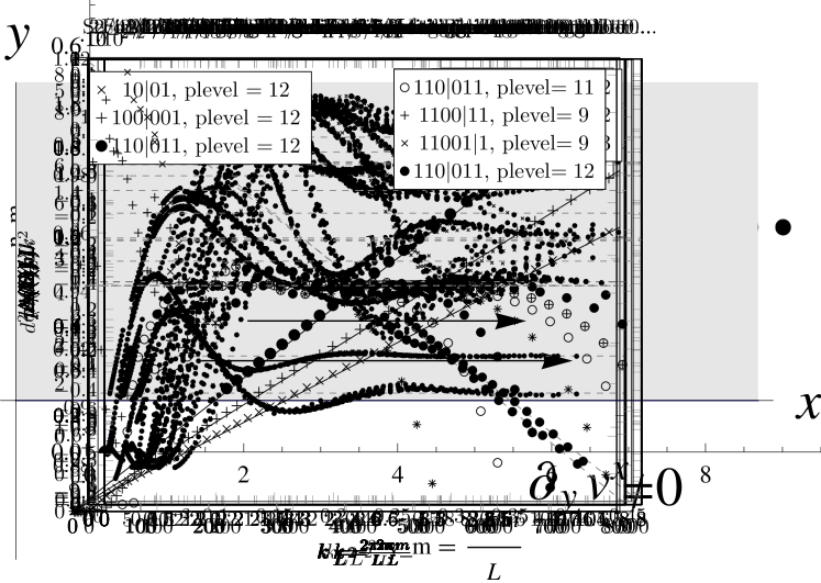
Figure 17: $p(k)/L$ in units of $-e/4\pi$ for $\nu=1/3$ Laughlin state. $(\times)$ for $N=14$ and $(\bullet)$ for $N=15$. $L=$ 12.5 to 22 with increments by 0.5. It converges to $1/3$.

Figure 18: $p(k)/L$ in units of $-e/4\pi$ for $\nu=1/4$ Laughlin state. $(\bullet)$ for $N=11$. $L=12.5$ to $22$ with increments by $0.5$. It converges to $3/8$.

Figure 19: $p(k)/L$ in units of $-e/4\pi$ for $\nu=2/2$ Moore-Read state.$(\times)$ for $N=18$ and $(\bullet)$ for $N=20$. $L=13$ to $20$ with increments by 0.5. It converges to $1/2$.

Figure 20: $p(k)/L$ in units of $-e/4\pi$ for $\nu=2/4$ Moore-Read state. $(\times)$ for $N=18$ and $(\bullet)$ for $N=20$. $L=16$ to $19.5$ with increments by 0.5. It converges to $1/2$.

IV Numerical Method.2 : Entanglement Spectrum

In Sec.IV.1, we introduce the orbital entanglement spectrum(OES)Li and Haldane (2008). We observe that the chirality of the OES can be explained by the fact the model states derives from Jack polynomials. Then, we describe how to calculate the total net momentum quantum number(“momentum polarization”) for a subsystem on a cylinder. We also derive the minimum change in the momentum quantum number as a function of the change in the particle number within a subsystem from the manipulation of root occupation numbers.

In Sec.IV.2, we relate the momentum polarization with the intrinsic dipole moment. We show that the momentum polarization can be decomposed into three distinct parts. We also show that one of the three which known as “topological spin” can be calculated solely from the root occupation numbers. The other topological term $\gamma=\tilde{c}-\nu$ is identified as a purely FQHE quantity which vanishes for IQHE.

In IV.3, we show that the momentum polarization calculated from the RES merely adds a trivial Landau-orbit contribution to the one calculated from the OES.

IV.1 Dipole moment of an ideal edge from orbital entanglement spectrum

We now describe another method to calculate the guiding center dipole moment using entanglement spectrum Li and Haldane (2008). This gives a connection between the chirality of entanglement spectrum and the dipole moment. We denote the full Fock space by $\mathcal{H}$, and represent it as a tensor product of two Fock spaces $\mathcal{H}_{L}$ and $\mathcal{H}_{R}$ so that $\mathcal{H}=\mathcal{H}_{L}\otimes\mathcal{H}_{R}$. Given a FQH ground state $|\Psi\rangle$ in the lowest Landau level, in order to find an orbital entanglement spectrum, it can be Schmidt decomposed

$$|\Psi\rangle=\sum_{r}e^{-(1/2)\xi_{r}}|\Psi_{L}^{r}\rangle\otimes|\Psi_{R}^{r}\rangle,$$ (38)

where $|\Psi^{r}_{R}\rangle\in\mathcal{H}_{L}$ and $|\Psi^{r}_{R}\rangle\in\mathcal{H}_{R}$. The set of real numbers $\xi_{r}$ are called the “entanglement spectrum”. Equivalently, the spectrum can be obtained by diagonalizing the density matrix of a subsystem

$$\rho_{L}=\frac{\sum_{r}e^{-\xi_{r}}|\Psi_{L}^{r}\rangle\langle\Psi_{L}^{r}|}{\sum_{r}e^{-\xi_{r}}}.$$ (39)

We place a FQH state on a cylinder, assigning guiding-center momenta. We then divide the whole system into two subsystems $L$ and $R$ depending on whether guiding-center momentum quantum number is either positive or negative. This is known as the “orbital cut”. The location of the cut (the zero momentum) does not matter in principle as long as it belongs to a “vacuum sector” if the number of particles is sufficiently large (We clarify what we mean by vacuum sector later in this section). However, in order to minimize the finite size effect, we should choose the cut to be located near the middle of the fluid as much as possible.

For instance, in the case of Laughlin 1/3 state with $N=8$ particles, we can divide the total system into subsystems as follows,

$$010010010010|010010010010$$

In this root occupation, there are $N_{L}^{0}=N_{R}^{0}=4$ particles in each system. Assigning zero to the cut, the total guiding-center quantum number is $M_{L}^{0}=-(\frac{3}{2}+\frac{9}{2}+\frac{15}{2}+\frac{21}{2})=-24$  for the left subsystem while the right subsystem has $M_{R}^{0}=-M_{L}^{0}$. These are called the “natural” values of $N_{L},\,N_{R},\,M_{L}$ and $M_{R}$. However, within the subsystem $L$, it can contain any non-negative number $N_{L}$ of particles as long as it satisfies $N_{L}+N_{R}=N$. Also, any total guiding-center quantum number $M_{L}$ is possible as long as it satisfies $M_{L}+M_{R}=0$. The entanglement spectrum obtained from this orbital cut splits into distinct sectors labeled by $N_{L}$ and $M_{L}$.

The chirality of the entanglement spectrum manifests itself when we note that the model FQH state derives from a Jack polynomials so that the many-particle state is spanned by the states obtainable by squeezing operation. Hence, the Laughlin state is a superposition of states with $M_{L}\geq M_{L}^{0}$ and $M_{R}\leq M_{R}^{0}$ :

$$|\Psi\rangle=\sum_{M_{L}\geq M_{L}^{0},N_{L},r^{\prime}}e^{-(1/2)\xi_{r^{\prime},N_{L},M_{L}}}|\psi_{L}^{r^{\prime},N_{L},M_{L}}\rangle\otimes|\psi_{R}^{r^{\prime},N_{R},M_{R}}\rangle,$$ (40)

where $\{r^{\prime}\}$ are the remaining labels of states. Thus, the change in total guiding-center quantum number $\Delta M_{L}=M_{L}-M_{L}^{0}$ is always non-negative for any pseudo-energies $\xi_{r}$. We also define $\Delta N_{L}=N_{L}-N_{L}^{0}$.

Now, we can calculate the expectation value of $\Delta M_{L}$

$$\langle\Delta M_{L}\rangle=\frac{\sum_{r^{\prime},N_{L},M_{L}}\Delta M_{L}e^{-\xi_{r^{\prime},N_{L},M_{L}}}}{\sum_{r^{\prime},N_{L},M_{L}}e^{-\xi_{r^{\prime},N_{L},M_{L}}}}.$$ (41)

We note that the lower bound of $\Delta M_{L}$ is determined by $\Delta N_{L}$. For instance, consider the following root occupation,

$$010010010010|01...$$

By squeezing, we can pull the extra particle on the right side of the cut and obtain a state in the left subsystem with $\Delta N_{L}=1$ and $\Delta M_{L}=3/2$ because the shown part of the root occupation has the total guiding-center quantum number $M_{L}^{0}+3/2$ and the squeezing operation does not change the total guiding-center quantum number. Now, consider the root occupations

$$010010010010|01001...$$

$$010010010000|00000...$$

By similar reasoning, we can obtain a state in the left subsystem with $\Delta N_{L}=2$ and $\Delta M_{L}=3/2+9/2$. When $\Delta N_{L}=-1$, it corresponds to the absence of an electron with the guiding-center quantum number $-3/2$, and thus $\Delta M_{L}=3/2$. For $1/q$ Laughlin ground states, with these observations, we can express the quantum number $\Delta M_{L}$ measured with respect to the “vacuum” cut as

$$\Delta M_{L}=\frac{q}{2}(\Delta N_{L})^{2}+\sum_{m=0}^{\infty}mb_{m}^{\dagger}b_{m},$$ (42)

where the boson number operator $b_{m}^{\dagger}b_{m}$ in the second term can take any non-negative integer values, and it describes additional increments in $\Delta M_{L}$ when the squeezing between a particle in the left subsystem and another in the right subsystem does not cause any further change of particle numbers in each subsystem. This is exactly the free chiral boson HamiltonianWen (1991).

By the same method, we can deduce that for 2/4 Moore-Read ground state, $\Delta M_{L}$ takes a specific form

$$\Delta M_{L} =\frac{2}{2}(\Delta N_{L})^{2}+\sum_{m=0}^{\infty}mb_{m}^{\dagger}b_{m}+\sum_{m=1/2}^{\infty}mf_{m}^{\dagger}f_{m}$$

$$(-1)^{\Delta N_{L}}=(-1)^{\sum_{m}f_{m}^{\dagger}f_{m}},$$ (43)

where the second term is the chiral boson contribution, and the last term is the chiral Majorana fermion contribution. The fermion momenta are half-integers, and the fermion occupation numbers are either 0 or 1. The second line is a constraint on the total number of Majorana fermions. For example, the minimum change of the total quantum number is $\Delta M_{L}=1+1/2$ when $\Delta N_{L}=1$.

IV.2 Decomposition of $\langle\Delta M_{L}\rangle$ and $\langle\Delta N_{L}\rangle$

We relate $\langle\Delta M_{L}\rangle$ to the total guiding-center momentum $P_{x}$ of the left subsystem

$$P_{x}=\frac{2\pi\hbar}{L}\langle\Delta M_{L}\rangle.$$

Furthermore, we relate the momentum to the dipole moment.

$$p^{y}=\frac{-e\ell_{B}^{2}}{\hbar}P_{x}=\frac{-2\pi\ell_{B}^{2}e}{L}\langle\Delta M_{L}\rangle.$$ (44)

We now show the equivalence of this dipole moment with that we calculated using occupation numbers. We can re-write the total guiding-center quantum number $M_{L}$ as

$$M_{L}=\sum_{m\in L}m\,n_{m},$$ (45)

where $m$’s are the guiding-center quantum numbers that belong to the left subsystem, and $n_{m}$’s are the electron occupation number operators. Meanwhile, $M_{L}^{0}$ is just a number that depends on the root occupation numbers $\{n_{m}^{0}\}$ of the model FQHE state

$$M_{L}^{0}=\sum_{m\in L}m\,n_{m}^{0}.$$ (46)

Then, the expectation value $\langle\Delta M_{L}\rangle$ is written as

$$\langle\Delta M_{L}\rangle =\text{Tr}_{L}\left[\Delta M_{L}\rho_{L}\right]$$

$$=\left(\sum_{m\in L}m\langle n_{m}\rangle_{0}-\bar{M}_{L}\right)-(M_{L}^{0}-\bar{M}_{L}),$$ (47)

where $\bar{M}_{L}=-\nu m_{F}^{2}/2$ is the total guiding-center quantum number for the left subsystem with the uniform number density $\nu$. The first term is the intrinsic dipole moment calculated previously. We denote the second term as

$$h_{\alpha}=M_{L}^{0}-\bar{M}_{L}.$$ (48)

$h_{\alpha}$ depends on the location of the cut. Similarly, we define $N_{L}^{0}=\sum_{m\in L}n_{m}^{0}$ and $\bar{N}_{L}=\nu|m_{F}|$. Then, $\langle\Delta N_{L}\rangle$ can be written as

$$\langle\Delta N_{L}\rangle =\text{Tr}_{L}[\Delta N_{L}\rho_{L}]$$ (49)

$$=\left(\sum_{m\in L}\langle n_{m}\rangle_{0}-\bar{N}_{L}\right)-(N_{L}^{0}-\bar{N}_{L}).$$ (50)

The first term vanishes by Luttinger’s theorem.

We denote the second term as

$$q_{\alpha}=N_{L}^{0}-\bar{N}_{L}.$$ (51)

We can calculate $h_{\alpha}$ and $q_{\alpha}$ for different model FQH states only using the root occupation numbers. For 1/3 Laughlin state, consider following different locations of cuts corresponding to quasi-particle, vacuum and quasi-hole sectors respectively,

$$01001001001|001001... h_{p}=1/6 q_{p}=1/3$$

$$010010010010|01001... h_{\mathbb{I}}=0 q_{\mathbb{I}}=0$$

$$0100100100100|1001... h_{h}=1/6 q_{h}=-1/3$$ .

For 1/5 Laughlin state, consider following different locations of cuts corresponding to two and one quasi-particles, vacuum, one and two quasi-hole sectors respectively,

$$010000100001|0000100001... h_{2p}=2/5 q_{2p}=2/5$$

$$0100001000010|000100001... h_{p}=1/10 q_{p}=1/5$$

$$01000010000100|00100001... h_{\mathbb{I}}=0 q_{\mathbb{I}}=0$$

$$010000100001000|0100001... h_{h}=1/10 q_{h}=-1/5$$

$$0100001000010000|100001... h_{2h}=2/5 q_{2h}=-2/5$$ .

For $2/4$ Moore-Read ground state, we have the following possibilities of cuts corresponding to isolated fermion, quasi-particle pair, vacuum and quasi-hole pair sectors respectively,

$$0110011001|100110... h_{\psi}=1/2 q_{\psi}=0$$

$$01100110011|00110... h_{2p}=1/4 q_{2p}=1/2$$

$$011001100110|0110... h_{\mathbb{I}}=0 q_{\mathbb{I}}=0$$

$$0110011001100|110... h_{2h}=1/4 q_{2h}=-1/2$$ .

For $2/4$ Moore-Read state with a quasi-hole at the left Fermi surface,

$$010101010101|0101... h_{p}=1/16 q_{p}=1/4$$

$$0101010101010|101... h_{h}=1/16 q_{h}=-1/4$$ .

We see that $h_{\alpha}$ are exactly the conformal spins of the elementary excitations ($h_{\alpha}$ were called “topological spin” by other authorsTu et al. (2013); Zaletel et al. (2013). $q_{\alpha}$ are the fractional charge of the elementary excitations.

In $\langle\Delta M_{L}\rangle$, the most dominant term is proportional to the squared circumference $L^{2}$. We define the sub-leading term as

$$\frac{\gamma}{24}-h_{\alpha}=\langle\Delta M_{L}\rangle+\frac{1}{2}\left(\frac{L}{2\pi\ell_{B}}\right)^{2}\frac{s}{q}$$ (52)

In order to calculate this sub-leading term, we need a large system. We generated orbital entanglement spectra for 1/3 Laughlin state, 1/5 Laughlin state and 2/4 Moore-Read state using the “matrix product state” program developed by Regnault et alEstienne et al. (2013). Each state contains 100 particles. Their accuracy is limited by the so-called “truncation level” (which we call plevel in the figures). As the truncation level increases the approximation to the exact state gets better. We plot the $\langle\Delta M_{L}\rangle$ against different values of circumference in Fig.21. The sub-leading term $\gamma/24$ is also plotted in Fig.22, 23 and 24. The numerical calculation is consistent with the predictionHaldane and Park that $\gamma$ may be expressed as

$$\gamma=\tilde{c}-\nu$$ (53)

where $\tilde{c}$ is the total signed central charge $c-\bar{c}$ of the underlying edge theory: $\tilde{c}=1$ for Laughlin states and $\tilde{c}=3/2$ for 2/4 Moore-Read state.

The theoretical derivation of this result will be presented elsewhereHaldane and Park . It is the anomaly of the signed Virasoro algebraHaldane and Park , with generators $\tilde{L}_{m}$ = $L_{m}-\bar{L}_{-m}$, which are the Fourier components of the momentum density; this survives as a universal algebra, with no renormalization, despite the breaking of Lorentz and conformal invariance when the various linearly-dispersing modes acquire different propagation speeds. Note that integer quantum Hall states, where the effect is due to simple filling of Landau levels by the Pauli principle (and which are not topologically ordered) do not exhibit a gapless “orbital” entanglement spectrum of the type discussed here, and have $\tilde{c}-\nu$ = 0. The anomaly $\tilde{c}$ appears in (53) as a “Casimir momentum” , which is a feature of chiral theories: this remains universal so long as translational invariance is unbroken, while the Casimir energy (the origin of the finite-size correction in non-chiral cft) becomes non-universal once Lorentz invariance is lost.

Figure 21: Dots represent $\langle\Delta M_{L}\rangle$ of 1/3 Laughlin ($\times$), 1/5 Laughlin (+) and 2/4 Moore-Read ($\bullet$) states for different values of circumference $L$ calculated from the orbital entanglement spectra with the truncation level equal to 12. Here, each orbital cut is a vacuum cut, $h_{\alpha}=0$. Each line represents the dominant value $L^{2}/(8\pi^{2}\ell_{B}^{2})\times(-s/q)$ where $-s/q=1/3,\,2/5,\,1/2$ respectively.

Figure 22: The plot of sub-leading term $\gamma/24$ for 1/3 Laughlin state. $\circ$: vacuum cut with truncation level 12. +: quasi-hole cut with truncation level 12. $\bullet$: vacuum cut with truncation level 13. The horizontal line represents 1/36.

Figure 23: The plot of sub-leading term $\gamma/24$ for 1/5 Laughlin state. $\circ$: vacuum cut with truncation level 13. +: one quasi-hole cut with truncation level 12. $\times$: two quasi-hole cut with truncation level 12. $\bullet$: vacuum cut with truncation level 16. The horizontal line represents 1/30.

Figure 24: The plot of sub-leading term $\gamma/24$ for 2/4 Moore-Read state. $\circ$: vacuum cut with truncation level 11. +: one quasi-hole cut with truncation level 9. $\times$: isolated fermion cut with truncation level 9. $\bullet$: vacuum cut with truncation level 12. The horizontal line represents 1/24.

IV.3 Momentum polarization from the real-space cut

The “orbital-cut” entanglement spectrum only has a gapless spectrum when it is applied to states with topological order. In particular, it does not show a gapless spectrum when applied to integer quantum Hall states, which are not topologically-ordered (they do not exhibit a topological ground-state degeneracy when constructed on surfaces on genus $>0$, which is the defining property of “topological order”). Dubail et al.Dubail et al. (2012) perceived this feature as a defect of the orbital-cut method, and introduced a modified “real-space” entanglement spectrum for quantum Hall states as a remedy. (However, it should be noted that the absence of a gapless orbital-cut entanglement spectrum in the trivial integer QHE case is consistent with Li and Haldane’s claimLi and Haldane (2008) that a gapless spectrum is a characteristic property of a topologically-ordered state.)

In the high field limit, quantum Hall states in Landau levels become an unentangled product of the state of the guiding-centers $\bm{R}_{i}$ and the Landau orbit (cyclotron motion) radii $\tilde{\bm{R}_{i}}$. Each Landau level is characterized by a form-factor

$$f_{n}(\bm{q})=\langle\psi_{n}|e^{i\bm{q}\cdot\tilde{\bm{R}}}|\psi_{n}\rangle_{L}=1-\tilde{\Lambda}_{n}^{ab}q_{a}q_{b}\ell_{B}^{2}+O(q^{4}),$$ (54)

where $|\psi_{n}\rangle_{L}$ is the $n$-th Landau level single-particle state. If only a single Landau level is occupied, the electronic state is a simple product of the guiding center state used in the “orbital cut” with a trivial completely-symmetric state of the Landau-orbit radii, characterized by a form factor $f(\bm{q})$ = $f(q_{x},q_{y})$. (This is the type of state for which the “real-space cut” was constructed in Dubail et al. (2012).) In the “Landau gauge”, the wavefunctions $\phi_{m}(x,y)$ have a profile

$$|\phi_{n,m}(x,y)|^{2}=\frac{1}{L}\int_{-\infty}^{\infty}\frac{dq_{y}}{2\pi}f_{n}(0,q_{y})e^{iq_{y}(y-y_{m})},$$ (55)

where $y_{m}$ = $2\pi m\ell_{B}^{2}/L$, $m\in\mathbb{Z}+1/2$. The real-space cut at $y=0$ is based on the partition

$$P^{L}_{n,m}=\int_{-\infty}^{0}dy\int_{0}^{L}dx|\phi_{n,m}(x,y)|^{2},\quad P^{L}_{n,m}+P^{R}_{n,m}=1.$$ (56)

Note also that

$$\sum_{m>0}mP_{n,m}^{L}-\sum_{m<0}mP^{R}_{n,m}=\sum_{m}m(P_{n,m}^{L}-\theta(m))$$

$$\quad=\frac{\tilde{\Lambda}_{n}^{yy}L^{2}}{(2\pi\ell_{B})^{2}}+\frac{1}{24}+\mathcal{O}(L^{-1}).$$ (57)

where for Galilean-invariant Landau levels with an effective mass tensor $m\tilde{g}_{ab}$ (with $\det\tilde{g}$ = 1),

$$\tilde{\Lambda}_{n}^{ab}=\frac{1}{2}\tilde{s}_{n}\tilde{g}^{ab}.$$ (58)

In order to obtain the dipole moment from the real-space cutDubail et al. (2012), we first double the single-particle Hilbert space $\mathcal{H}_{1}$ on a cylinder into two subspaces $\mathcal{H}_{1L}$ and $\mathcal{H}_{1R}$ where a new “pseudospin” index that takes values “$R$” and “$L$” has been introduced:

$$\mathcal{H}_{1}\mapsto\mathcal{H}_{1L}\otimes\mathcal{H}_{1R}.$$ (59)

If a function $f(\bm{r})$ belongs to $\mathcal{H}_{1X}$, then $f(\bm{r})=0$ if $\bm{r}\not\in X$ where $X$ can be either the subsystem $L$ or $R$. We choose the line $x=0$ to be the boundary along the translational invariant direction so that the guiding-center remains as a good quantum number. Now, consider the Fock space $\mathcal{H}$. Denote a vacuum state with no particle by $|\text{vac}\rangle$. We create a particle with the guiding-center $m$ in $n$-th Landau level by $c_{n,m}^{\dagger}$. This creation operator can be decomposed as

$$c_{n,m}^{\dagger} =u_{n,m}c^{\dagger}_{n,m,L}+v_{n,m}c^{\dagger}_{n,m,R}$$ (60a)

$$|u_{n,m}|^{2} =P_{n,m}^{L},\quad|v_{n,m}|^{2}=P^{R}_{n,m},$$ (60b)

where the physical state satisfies the constraint

$$(v_{n,m}c_{n,m,L}-u_{n,m}c_{n,m,R})|\Psi\rangle=0,$$ (61)

so all occupied orbitals have a pseudospin which is fully-polarized in the “physical” direction. For notational convenience, we concentrate on a single Landau level and drop the index $n$. Given a Slater determinant state $|\{n_{m}\}\rangle$ labeled by occupation numbers $n_{m}$,

$$|\{n_{m}\}\rangle=\prod_{m}(c_{m}^{\dagger})^{n_{m}}|\text{vac}\rangle$$

$$=\prod_{m}\left(u_{m}c^{\dagger}_{m,L}+v_{m}c^{\dagger}_{m,R}\right)^{n_{m}}|\text{vac}\rangle$$ (62)

the product of creation operators can be expanded. Then, we obtain

$$|\{n_{m}\}\rangle=\sum_{\alpha,\beta:N_{L}+N_{R}=N}A_{\alpha\beta}(\{n_{m}\})|\Psi_{\alpha}^{L}\rangle\otimes|\Psi_{\beta}^{R}\rangle$$ (63)

where $|\Psi_{\alpha}^{X}\rangle$ are Slater determinant states belonging to the Fock space $\mathcal{H}_{X}$ ($X=L,\,R$) and $A_{\alpha\beta}(\{n_{m}\})$ is a product of $u_{m}$ and $v_{m}$ . With this expansion, and after translating the partition $\lambda$ into the occupation numbers $\{n_{m}\}$, the mapping of a Jack polynomial into a model FQH state $|\Psi\rangle$ in (34) becomes

$$|\Psi\rangle=\sum_{\stackrel{{\scriptstyle\alpha,\beta}}{{N_{L}+N_{R}=N}}}\sum_{\{n_{m}\}\leq\{n_{m}^{0}\}}a_{\{n_{m}\}}A_{\alpha\beta}(\{n_{m}\})|\Psi_{\alpha}^{L}\rangle\otimes|\Psi_{\beta}^{R}\rangle$$ (64)

We can further Schmidt-decompose the model FQH state $|\Psi\rangle$. However, if our objective is only to calculate the diagonal operators such as $M_{L}$ and $N_{L}$, the information we gathered from the orbital cut is enough. Consider the expectation value of the operator $n_{m}^{L}=c^{\dagger}_{m,L}c_{m,L}$

$$\langle n_{m}^{L}\rangle^{\prime}=\text{Tr}_{L}[c_{m,L}^{\dagger}c_{m,L}\rho_{L}^{\prime}]$$ (65)

where $\rho_{L}^{\prime}$ is the normalized density matrix for the subsystem $L$, and we placed an apostrophe on the bracket $\langle...\rangle^{\prime}$ to distinguish the real-space cut expectation value with the orbital cut expectation value $\langle...\rangle$. For all guiding-centers $m^{\prime}$ such that $m^{\prime}\neq m$, the factors $P_{m^{\prime}}^{L}$ and $P_{m^{\prime}}^{R}$ appear in pairs in the expectation value, and add to one. From this observation, we see that the expectation value simplifies to

$$\langle n_{m}^{L}\rangle^{\prime}=P_{m}^{L}\langle n_{m}\rangle_{0}$$ (66)

Using this expression, in the expectation value of $\Delta M_{L}$,

$$\langle\Delta M_{L}\rangle^{\prime} =\sum_{m}m\langle n^{L}_{m}\rangle^{\prime}-M_{L}^{0}$$

$$=\sum_{m}m(P_{m}^{L}-\theta(m))\langle n_{m}\rangle_{0}$$

$$\quad+\sum_{m<0}m\langle n_{m}\rangle_{0}-M_{L}^{0}.$$ (67)

The first term is an additional term that appears when we consider the real-space cut. The second term is the expectation value of $\Delta M_{L}$ with the orbital cut that we calculated previously. In the first term, $P_{m}^{L}$ $\rightarrow 1$ for $m\ll 0$, and the summand vanishes. Meanwhile, as $m\rightarrow 0$, which is the location of the real-space cut, we are deep into the bulk so that $\langle n_{m}\rangle_{0}=\nu$. Thus, in the thermodynamic limit, the expectation value $\langle\Delta M_{L}\rangle^{\prime}$ becomes

$$\langle\Delta M_{L}\rangle^{\prime} =\nu\sum_{m}m(P_{m}^{L}-\theta(m))+\langle\Delta M_{L}\rangle$$ (68)

The first term was already considered in (57).

For simplicity, we now assume Galilean-invariant Landau orbits, so $\tilde{\Lambda}_{n}^{yy}$ = ${\textstyle\frac{1}{2}}\tilde{s}_{n}\tilde{g}^{yy}$, where $\tilde{s}_{n}$ = $n+{\textstyle\frac{1}{2}}$ is the Landau-orbit spin. If we further include the contributions from the filled Landau levels 0,1,…,$n-1$, then $\langle\Delta M_{L}\rangle^{\prime}$ is

$$\langle\Delta M_{L}\rangle^{\prime}= \frac{1}{2}\left(\frac{L}{2\pi\ell_{B}}\right)^{2}\left(\sum_{n^{\prime}=0}^{n}\tilde{s}_{n^{\prime}}\nu_{n^{\prime}}\tilde{g}^{yy}-\frac{s}{q}g^{yy}\right)$$

$$+ \frac{(\nu^{\prime}+\gamma)}{24}+\mathcal{O}(L^{-1}),$$ (69)

where $\nu_{n^{\prime}}$ = $\tilde{c}_{n^{\prime}}$ = 1 for $n^{\prime}<n$ and $\nu_{n}=\nu$. We also defined $\nu^{\prime}=\sum_{n^{\prime}=0}^{n}\nu_{n^{\prime}}$ and $\gamma$ = $\tilde{c}_{n}-\nu_{n}$. We explicitly wrote the two metrics $g_{ab}$ and $\tilde{g}_{ab}$ since they need not coincide as noted before Haldane (2011). There are topological contributions from each cut: we get $n/24$ from $n$ filled Landau levels and $\nu/24$ from the partially filled Landau level as a result of the real-space cut. We get $\gamma/24$ from the variation of orbital occupations near the physical edge. The normal vector of the surface of the fluid at the physical edge is reversed from the normal vector at the real-space cut. We note here that the Landau-orbit spins $\tilde{s}_{n^{\prime}}$ ($n^{\prime}=0,\dots,n$) are positive while the guiding-center spin $s$ is negative. The general expression for the total Hall viscosity tensor $\eta_{H}^{\prime ab}$ (the sum of the Landau-orbit ant guiding-center contributions) is

$$\eta_{H}^{\prime abcd}= {\textstyle\frac{1}{2}}\left(\eta_{H}^{\prime ac}\epsilon^{bd}+\eta_{H}^{\prime bd}\epsilon^{ac}+\eta_{H}^{\prime bc}\epsilon^{ad}+\eta_{H}^{\prime ad}\epsilon^{bc}\right)$$ (70a)

$$\eta_{H}^{\prime ab}= \frac{eB}{2\pi}\left(\sum_{n}\tilde{\Lambda}_{n}^{ab}\nu_{n}-\frac{1}{2}\frac{s}{q}g^{ab}\right),$$ (70b)

Using this expression for the Hall viscosity, we can write the momentum polarization in a fully covariant tensor form as

$$\langle\Delta M_{L}\rangle^{\prime}=\hbar^{-1}\eta^{\prime ab}_{H}\epsilon_{ac}\epsilon_{bd}\frac{L^{c}L^{d}}{2\pi\ell_{B}^{2}}+\frac{(\nu^{\prime}+\gamma)}{24}$$ (71)

The $O(L^{2})$ term gives the Hall viscosity, which is now the sum of two terms: one is derived from the Landau-orbit form factors, weighted by the Landau level occupation, and the other is the guiding-center contribution derived from the orbital cut.

We note the the “real-space cut” involves far greater computational effort than the “orbital cut”, but at least as far as the “momentum polarization” is concerned, merely adds trivial contributions to the Hall viscosity and topological terms e.g., $(\tilde{c}-\nu)+\nu=\tilde{c}$. Clearly all the non-trivial topological and entanglement information of the topologically-ordered states is fully present in the “orbital-cut”. From this viewpoint, we are tempted to conclude that use of the “real-space cut” is an unnecessary use of computational resources that merely serves to conceal the structures of the “orbital cut” entanglement spectrum by convoluting them with the form-factor of the Landau orbits.

V Conclusion

We showed that the intrinsic dipole moment along the edges of the incompressible FQH fluids can be expressed in terms of electric charge $e$, guiding center spin $s$, number of fluxes per a composite boson $q$, confirming the prediction made in the previous work Haldane (2009). This provides another sum rule for the FQH fluids in addition to the Luttinger sum ruleLuttinger (1960). For incompressible FQH states, the electric force on the intrinsic dipole moment is balanced the stress given by the gradient of the flow velocity times the guiding-center Hall viscosity.

We also related the the edge dipole moment to the expectation value of the momentum (or “momentum polarization”Tu et al. (2013)) of the entanglement spectrum. In the high-field limit, when the guiding-center and Landau-orbit degrees of freedom become unentangled with each other, the dipole moment and the related Hall viscosity separate cleanly into independent parts respectively coming from the non-trivial correlated guiding-center degrees of freedom of the FQH state, and the trivially-calculable one-body properties of the Landau orbits. The “orbital cut” entanglement spectrum introduced by Li and HaldaneLi and Haldane (2008) contains only information on the guiding-center degrees of freedom, and allows the guiding-center contribution to the Hall viscosity of the FQH fluid to be found as a bulk geometric property, and also gives the topological quantity $\gamma$ = $\tilde{c}-\nu$, the difference between the (signed) “conformal anomaly” (or “chiral stress-energy anomaly”Haldane and Park $\tilde{c}$ = $c-\bar{c}$, and the chiral charge anomaly $\nu$, which are the two fundamental quantum anomalies of the FQH fluids. It is useful to note that $\gamma$ is insensitive to completely-filled Landau levels, and vanishes identically in integer quantum Hall states, which do not exhibit topological-order.

We also examined the equivalent calculation in the “real-space” entanglement spectrum described by Dubail et al.Dubail et al. (2012), which adds information about the Landau orbit to provide the combined guiding-center plus Landau-orbit contribution to the Hall viscosity and $\tilde{c}$ rather than $\gamma$. However since the “real-space entanglement” method involves much extra computational complexity, and convolutes the non-trivial Landau-orbit-independent correlated guiding center data with the essentially trivial (and Landau-level-dependent) Landau-orbit form factor data, we concluded that there were no advantages to use of the “real-space” as opposed to “orbital” entanglement spectrum. Indeed, since the Landau-orbit form factor is essentially unrelated to the FQH correlations, and can be chosen as an additional (and arbitrary) ingredient to convert orbital entanglement data into a “real-space” form, its use may actually serve to conceal the essential features of the guiding-center entanglement. The “real-space” spectrum may also be thought of operationally as the use of an essentially ad-hoc function $P^{L}_{m}$ (56) that can be arbitarily chosen to “smear out” a sharp orbital cut between cylinder orbitals $m$ and $m+1$, which breaks both guiding-center indistiguishability (by introducing “pseudo-spin” labels “$L$” and “$R$”) and reducing the full 2D translational symmetry (the parallel to the cylinder axis (in the $N\rightarrow\infty$ limit, or equivalently, full rotational symmetry in the spherical geometry) to 1D axial translational symmetry. It interpolates continuously between two completely-well-defined limits of guiding-center entanglement: the “orbital cut” which preserves guiding-center indistinguishability while breaking 2D translational symmetry down to 1D translational symmetry, and the “particle cut” which divides the guiding centers into two distinguishable groups, but preserves full 2D translational symmetry.

Acknowledgements: This work was supported in part by the Department of Energy, Office of Basic Energy Sciences through grant No. DE-SC0002140 and also by the W. M. Keck foundation.

References

- Tsui et al. (1982) D. C. Tsui, H. L. Stormer, and A. C. Gossard, Phys. Rev. Lett. 48, 1559 (1982).
- Avron et al. (1995) J. E. Avron, R. Seiler, and P. G. Zograf, Phys. Rev. Lett. 75, 697 (1995).
- Read (2009) N. Read, Phys. Rev. B 79, 045308 (2009).
- Read and Rezayi (2011) N. Read and E. H. Rezayi, Phys. Rev. B 84, 085316 (2011).
- Haldane (2009) F. D. M. Haldane, (2009), arXiv:0906.1854 .
- Haldane (2011) F. D. M. Haldane, Phys. Rev. Lett. 107, 116801 (2011).
- Hoyos and Son (2012) C. Hoyos and D. T. Son, Phys. Rev. Lett. 108, 066805 (2012).
- Maciejko et al. (2013) J. Maciejko, B. Hsu, S. A. Kivelson, Y. Park, and S. L. Sondhi, Phys. Rev. B 88, 125137 (2013).
- Bradlyn et al. (2012) B. Bradlyn, M. Goldstein, and N. Read, Phys. Rev. B 86, 245309 (2012).
- Li and Haldane (2008) H. Li and F. D. M. Haldane, Phys. Rev. Lett. 101, 010504 (2008).
- Zaletel et al. (2013) M. P. Zaletel, R. S. K. Mong, and F. Pollmann, Phys. Rev. Lett. 110, 236801 (2013).
- Tu et al. (2013) H.-H. Tu, Y. Zhang, and X.-L. Qi, Phys. Rev. B 88, 195412 (2013).
- Wen (1991) X. G. Wen, Phys. Rev. B 43, 11025 (1991).
- Bernevig and Haldane (2008) B. A. Bernevig and F. D. M. Haldane, Phys. Rev. Lett. 100, 246802 (2008).
- Dubail et al. (2012) J. Dubail, N. Read, and E. H. Rezayi, Phys. Rev. B 85, 115321 (2012).
- Laughlin (1983) R. B. Laughlin, Phys. Rev. Lett. 50, 1395 (1983).
- Zhang et al. (1989) S. C. Zhang, T. H. Hansson, and S. Kivelson, Phys. Rev. Lett. 62, 82 (1989).
- Landau and Lifshitz (1986) L. Landau and E. Lifshitz, Theory of Elasticity, 3rd (Pergamon Press, Oxford, UK, 1986).
- Moore and Read (1991) G. Moore and N. Read, Nucl. Phys. B 360, 362 (1991).
- Haldane (1983) F. D. M. Haldane, Phys. Rev. Lett. 51, 605 (1983).
- Wen and Zee (1992) X. G. Wen and A. Zee, Phys. Rev. Lett. 69, 953 (1992).
- Bernevig and Regnault (2009) B. A. Bernevig and N. Regnault, Phys. Rev. Lett. 103, 206801 (2009).
- Rezayi and Haldane (1994) E. Rezayi and F. Haldane, Phys. Rev. B 50, 17199 (1994).
- Luttinger (1960) J. M. Luttinger, Phys. Rev. 119, 1153 (1960).
- Haldane (1993) F. D. M. Haldane, Proceedings of the International School of Physics ”Enrico Fermi”, Course CXXI ”Perspectives in Many-Particle Physics” : Luttinger’s theorem and Bosonization of the Fermi surface (north-holland, Amsterdam, 1993) arXiv:cond-mat/0505529 .
- Varjas et al. (2013) D. Varjas, M. P. Zaletel, and J. E. Moore, Phys. Rev. B 88, 155314 (2013).
- Estienne et al. (2013) B. Estienne, Z. Papić, N. Regnault, and B. A. Bernevig, Phys. Rev. B 87, 161112 (2013).
- (28) F. D. M. Haldane and Y. Park, Unpublished.