Phenomenological model for charge dynamics and optical response of disordered systems: application to organic semiconductors.

Abstract

We provide a phenomenological formula which describes the low-frequency optical absorption of charge carriers in disordered systems with localization. This allows to extract, from experimental data on the optical conductivity, the relevant microscopic parameters determining the transport properties, such as the carrier localization length and the elastic and inelastic scattering times. This general formula is tested and applied here to organic semiconductors, where dynamical molecular disorder is known to play a key role in the transport properties. The present treatment captures the basic ideas underlying the recently proposed transient localization scenario for charge transport, extending it from the d.c. mobility to the frequency domain. When applied to existing optical measurements in rubrene FETs, our analysis provides quantitative evidence for the transient localization phenomenon. Possible applications to other disordered electronic systems are briefly discussed.

I Introduction

The semiclassical Bloch-Boltzmann transport theory, which relies on the existence of well-defined extended ”band” states that are weakly scattered by impurities and phonons, is known to provide a successful description of charge carrier dynamics in ordinary wide-band semiconductors. It has been shown in recent years Troisi06 ; Zuppi ; Ciuchi11 that such standard paradigm is not appropriate to organic semiconductors, which are more effectively described by taking the strong disorder limit as a starting point. The reason for this is that even in ultrapure crystalline samples where extrinsic sources of disorder are removed, large thermal molecular motions arise due to the weak van der Waals intermolecular binding. Such dynamical fluctuations in molecular positions and orientations strongly scatter the charge carriers, causing a breakdown of the assumptions underlying semiclassical transport.Friedman ; Cheng ; Fratini09 ; Ciuchi11 Unlike static disorder, however, dynamical disorder is unable to fully localize the carriers: after a transient localization regime which extends up to the typical timescale of molecular vibrations, a diffusive behavior is eventually established. It can be shown that the resulting d.c. mobility is a decreasing function of temperature, with a power-law behavior which resembles that of semiclassical ”band-like” carriers. Its modest value, however, at best of the order of a few tens of $cm^{2}/Vs$ at room temperature, is there to remind us of the presence of an underlying strong disorder.

A more direct signature of this unconventional transport mechanism is predicted in the a.c. response of the carriers: associated to the transient localization phenomenon, a peak emerges in the optical conductivity at a frequency related to the amount of molecular disorder, deeply modifying the usual Drude response expected for band-like carriers.Ciuchi11 ; Cataudella All these features — power-law temperature dependence, low values of the mobility and the existence of a localization peak in the optical conductivity — are commonly found in experiments on high-mobility organic semiconductors, giving support to the transient localization scenario for charge transport.

It is our aim here to derive a general phenomenological formula describing the low-frequency optical absorption of charge carriers in disordered systems with localization. Such a formula should be able to provide a theoretically simple description of the transient localization scenario for organic semiconductors, capturing the main features evidenced in recent numerical simulation studies. Rather than studying a particular microscopic model, as was done in Refs. Troisi06 ; Zuppi ; Fratini09 ; Ciuchi11 ; Cataudella ; Ciuchi12 , we therefore introduce a phenomenological model for the carrier dynamics which yields a closed analytical form for both the d.c. mobility and optical conductivity. Our model is able to interpolate between the Drude-like response of diffusive carriers and the absorption peak expected in the presence of strong Anderson localization, and establishes a direct connection between the temperature dependent mobility and the optical conductivity. We then perform a benchmarking of the phenomenological formula for the optical conductivity by comparing it with a true microscopic calculation of this quantity in a model system Ciuchi12 . Our analysis demonstrates that the formula derived here can be used to accurately extract the microscopic parameters governing the carrier dynamics, such as the transient localization length and the relevant scattering rates, and to estimate the electron-intermolecular vibration coupling strength and the amount of extrinsic (i.e. non-thermal) disorder. This allows us to analyze quantitatively the optical absorption spectra available in organic FETs in the framework of the transient localization scenario. In the conclusive section we briefly discuss how the present theory can be applied not only to organic semiconductors but also to bad metals and other disordered systems, including organic conductors and carbon nanotubes.

For readers not interested in the formal developments of the theory, the central formula of the paper which can be used to fit optical conductivity data in disordered semiconductors is presented in Sec. II D. An analogous formula valid for degenerate electron systems at low temperatures is given in Appendix C.

II Phenomenological model for the charge dynamics

II.1 General formalism

We start by briefly reviewing a recently developed theoretical framework Mayou88 ; Khanna ; Roche ; Mayou00 ; Triozon ; Trambly06 ; Ciuchi11 ; Ciuchi12 based on the Kubo formula, that relates the quantum diffusion of electrons and the optical conductivity. This formalism has been successfully applied to analyze the carrier dynamics in electronic systems where localization effects cause a breakdown of usual Boltzmann transport including quasicrystalsMayou00 ; Trambly06 , organic semiconductorsCiuchi11 ; Ciuchi12 , and graphene Trambly13 .

The key ingredient of such formalism is the quantum-mechanical spread $\Delta X^{2}(t)=\langle[\hat{X}(t)-\hat{X}(0)]^{2}\rangle$ of the position operator $\hat{X}(t)=\sum_{i=1}^{N}\hat{x}_{i}(t)$ of an N-electron system, which contains all the information on the electron dynamics over time. In particular, the first and second derivatives of the electronic spread yield respectively the instantaneous diffusivity,

$$\mathcal{D}(t)=\frac{1}{2}\frac{d\Delta X^{2}}{dt}=\frac{1}{2}\int_{0}^{t}C_{+}(t^{\prime})dt^{\prime}$$ (1)

and the retarded anticommutator velocity correlation function,

$$C_{+}(t)=\frac{d^{2}\Delta X^{2}}{dt^{2}}=\theta(t)\langle\{\hat{V}(t),\hat{V}(0)\}\rangle,$$ (2)

with the initial condition $\Delta X^{2}(t=0)=0$. Following Ref.Ciuchi12 , once that the time-dependent quantum-mechanical spread or equivalently the anticommutator velocity correlation function are known, the usual commutator correlation function that enters the Kubo response theory is obtained by imposing the detailed balance condition.Ciuchi12 The real part of the optical conductivity is then obtained as

$$\sigma(\omega)=\frac{e^{2}\tanh(\frac{\hbar\omega}{2k_{B}T})}{\hbar\omega\Omega}ReC_{+}(\omega)$$ (3)

where $e$ is the electron charge, $\Omega$ is the system volume and $C_{+}(\omega)=\int_{0}^{\infty}e^{i\omega t}C_{+}(t)dt$. A similar formula has been proposed in Ref. Lindner10 to account for the bad metallic behavior in a system of hard-core bosons.

In the following sections we shall focus on the non-degenerate low-density limit appropriate to weakly doped semiconductors. In this case the correlation function $C_{+}(t)$ as well as the quantum spread are directly proportional to the number of carriers $N$, being thermodynamical averages for $N$ independent particles. We present a phenomenological ansatz for the correlation function $C_{+}(t)$ and the quantum diffusion of electrons in organic semiconductors and derive the corresponding optical conductivity lineshape. The modifications of the formalism which apply to degenerate electron systems are presented in Appendix C.

II.2 Localized carriers

Our starting point is the following reference model, that accounts for carrier localization in the limit of strong static disorder (from now on we shall always refer to the anticommutator velocity correlation function and drop the subscript $+$ for simplicity):

$$C(t)=\frac{C(0)}{1/\tau-1/\tau_{b}}\left[\frac{1}{\tau}e^{-t/\tau}-\frac{1}{\tau_{b}}e^{-t/\tau_{b}}\right]$$ (4)

$$\Delta X^{2}(t)=\frac{C(0)}{1/\tau-1/\tau_{b}}\left[\tau_{b}(1-e^{-t/\tau_{b}})-\tau(1-e^{-t/\tau})\right].$$ (5)

The correlation function in Eq. (4) consists of two terms. A first exponential decay causes relaxation of the velocity on a timescale given by the elastic scattering time $\tau$. This is equivalent to the usual decay term which is present in the semiclassical Boltzmann theoryGruner , and which is responsible for the Drude response of the carriers (see below and Appendix A). A second ”backscattering” term, with a timescale $\tau_{b}>\tau$, is introduced in order to describe the negative velocity correlations which lead to electron localization at long times. The choice of the prefactors of the exponential terms between brackets ensures that the diffusivity vanishes at long times, $\int_{0}^{\infty}C_{+}(t^{\prime})dt^{\prime}=2\mathcal{D}(t\to\infty)=0$. This function is illustrated in Fig. 1-a (dotted line). note-geometrical

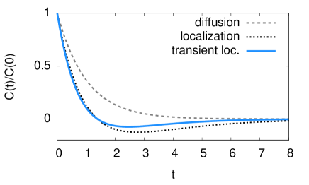
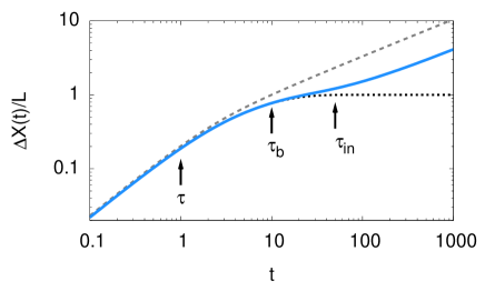
Figure 1: (a) The velocity correlation function $C(t)$ obtained from the phenomenological RTA for full localization [Eq.(4), black dotted line] and transient localization [Eq.(8), full blue line]. We have taken $\tau=1$, $\tau_{b}=2$ and $\tau_{in}=5$ (times are in units of $\tau$). The diffusive term alone with $\tau=1$ is shown for comparison [first term in Eq.(4), dashed gray line]; (b) The corresponding quantum spread $\Delta X(t)$ per particle, in units of the localization length $L$. For illustrative purposes, we have taken here $\tau=1$, $\tau_{b}=10$ and $\tau_{in}=50$ (note the logarithmic scale on the time axis). Arrows indicate the three characteristic timescales (elastic scattering, backscattering and inelastic).

The expression Eq. (5) of the quantum diffusion follows from double integration of Eq. (4). It describes three different regimes expected in a localized N-electron system in different time ranges, as illustrated in Fig. 1-b (dotted line): a ballistic evolution, $\Delta X^{2}(t)=C(0)t^{2}/2$, at initial times is followed by diffusion, $\Delta X^{2}(t)\propto t$, setting in after the elastic scattering time, $t>\tau$. The diffusive behavior is eventually destroyed by backscattering, causing electronic localization, $\Delta X^{2}(t)\to\mathrm{const}$, at $t>\tau_{b}$.

From that several relations can be derived whose physical content is particularly instructive. First of all, from Eq. (5), the value of the localization length, $L^{2}=\lim_{t\to\infty}\Delta X^{2}(t)/N$, fixes the diffusive behavior of the carriers prior to localization. By expanding Eq. (5) in the range $\tau<t<\tau_{b}$ we obtain $\Delta X^{2}(t)=2ND_{sc}(t-\tau)$, with $D_{sc}=L^{2}/(\tau_{b}-\tau)$ the semiclassical diffusivity.C0 Observing that generally $\tau_{b}\gg\tau$ we can rewrite this as $L\simeq\sqrt{D_{sc}\tau_{b}}$, which can be actually taken as a definition of the backscattering time: it is the time it takes to the electron spread to attain the localization length $L$ upon diffusing with a rate $D_{sc}$. Similarly, the elastic mean free path is $\ell=\sqrt{D_{sc}\tau}$, so that

$$\frac{L}{\ell}\simeq\sqrt{\frac{\tau_{b}}{\tau}}.$$ (6)

The ratio of the localization length to the elastic mean free path is actually known from the Thouless relationBeenakker : apart from numerical factors, it is equal to the number of conduction channels available in the system. For one-dimensional conduction with one orbital per unit cell, for example, the number of channels is one so that $L/\ell$ and $\tau_{b}/\tau$ are both constant and independent of the disorder strength (cf. Sec. III below). For anisotropic two-dimensional systems, one can roughly apply an analogous argument by defining an effective width $L_{\perp}$ , which corresponds to the localization length along the transverse direction. The effective number of modes in this case is therefore of the order of $L_{\perp}/a_{\perp}$, and so is the ratio $\sqrt{\tau_{b}/\tau}$.

A second useful relation follows from the observation that, for independent non-degenerate particles of mass $m^{*}$, the semiclassical diffusivity along a given direction is known and given by $D_{sc}=2k_{B}T\tau/m^{*}$ (see Appendix A). Equating this to the expression given before Eq. (6) yields

$$L^{2}=\frac{2k_{B}T}{m^{*}}\tau(\tau_{b}-\tau).$$ (7)

This relation shows that the localization length $L$ and the backscattering time $\tau_{b}$, i.e. the two parameters governing the localization process, are not independent. The validity of both Eq. (6) and Eq. (7) will be verified numerically in Sec. III, and their practical relevance when fitting experimental data will be demonstrated in Sec IV.

II.3 Transient localization and d.c. mobility within the RTA

In organic semiconductors, the dynamical nature of molecular disorder prevents localization of the carriers at long times. A recovery of carrier diffusion is expected in the case of dynamical disorder because the time fluctuations of the disorder potential destroy the quantum interferences responsible for carrier localization. This effect, which occurs on the typical timescale of molecular motions, that we denote $\tau_{in}$, can be included in our phenomenological model in the spirit of the RTA by setting:

$$C_{RTA}(t)=C(t)e^{-t/\tau_{in}}.$$ (8)

We assume that the inelastic timescale is the longest timescale in the problem, $\tau_{in}>\tau_{b}>\tau$. This is a reasonable assumption in organic semiconductors because the molecular motions that are at the origin of disorder are slow, owing to the large molecular mass and the weak inter-molecular (van der Waals) restoring forces. The consequence of this assumption is that the behavior of the system at the timescales relevant for the buildup of localization is very similar to that of the reference case with static disorder, Eq. (4). The main effect of the extra exponential decay in Eq. (8) is to suppress the long-time backscattering [the second term in Eq. (4)], restoring carrier diffusion at long times note-geometrical . This is best seen in the quantum spread $\Delta X^{2}(t)$, which is readily obtained by integrating Eq. (8) twice over time (see Appendix B for the full expression). As shown in Fig. 1-b (full line), the inclusion of the disorder dynamics causes a departure from the behavior of the reference localized system on a scale $t\sim\tau_{in}$. This form qualitatively agrees with the quantum spread obtained via quantum-classical simulations of a model with dynamical inter-molecular disorder (see e.g. Fig.1 in Ref.Ciuchi11 ).

Importantly, when velocity correlations are allowed to relax via Eq. (8) a diffusive behavior is recovered at long times, with a diffusion constant given by:

$$D\simeq\frac{L^{2}}{2\tau_{in}}.$$ (9)

where we have assumed $\tau_{in}\gg\tau_{b},\tau$ (see again Appendix B for a more general expression). The form Eq. (9) has a clear physical meaning: it corresponds to the diffusion of particles hopping on a lengthscale $L$ with a jump rate $1/\tau_{in}$. The corresponding mobility is obtained from Einstein’s relation as Zuppi ; Ciuchi11 ; Ciuchi12

$$\mu(T)\simeq\frac{e}{k_{B}T}\frac{L^{2}(T)}{2\tau_{in}}.$$ (10)

It has been shown in Refs. Ciuchi11 ; Ciuchi12 that, if we consistently associate $\tau_{in}$ with the typical frequency of the relevant inter-molecular vibrations, $1/\tau_{in}\simeq\omega_{0}$, Eq. (10) correctly describes both the absolute value and temperature dependence of the mobility observed in crystalline organic semiconductors in the intrinsic regime. In this case $L$ is a smoothly decreasing function of $T$ because the main source of disorder is constituted by molecular motions of thermal origin, and the localization length decreases upon increasing the amount of disorderZuppi ; Fratini09 ; Ciuchi12 . This leads to an overall power-law temperature dependence of the mobility, which is a common feature observed in pure samples at sufficiently high temperatures.

The power-law temperature dependence described above should not be confused with standard semi-classical transport: the transient localization form Eq. (10) of the mobility is very different from the usual semiclassical ”Drude” form, $\mu(T)=\frac{e\tau(T)}{m}$, because it arises from a fundamentally different microscopic mechanism. As can be seen in Fig. 1-b, the diffusivity in the presence of transient localization (full line) is generally lower than that of semiclassical carriers (dashed line; see also the $\omega\to 0$ limit in Fig. 2). It is then easy to understand that Eq. (10) can describe mobilities that go below the so-called Mott-Ioffe-Regel limit $\mu_{0}\approx ea^{2}/\hbar$, which is where the apparent mean-free path falls below the typical inter-molecular distance, implying a breakdown of the semiclassical approximation. Organic semiconductors are a particularly favorable ground for this breakdown to occur, because of the large thermal molecular disorder (leading to a short $L$) together with large values of the molecular mass (implying a large $\tau_{in}$), both contributing to reduce the value of $\mu$ in Eq. (10). Indeed, observing that $L$ reduces to few lattice spacings at room temperature even in pure samples (see Refs. Fratini09 ; Ciuchi12 and Fig. 4 below), a sufficient condition for the breakdown of the semi-classical limit is that $\hbar/\tau_{in}<k_{B}T$, which is easily reached in these compounds. The quantitative microscopic calculations of Ref. Ciuchi12 (see Fig. 2-a there, where the mobility is conveniently expressed in units of $\mu_{0}$) do confirm that the Mott-Ioffe-Regel limit is attained in pure samples around room temperature, and that the mobility always lies below this limit when sizable extrinsic disorder is present.

II.4 Drude-Anderson model for the optical conductivity

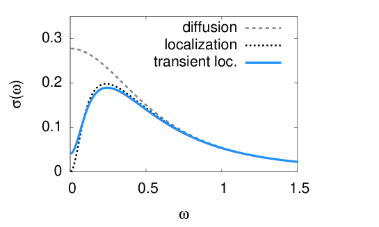
Figure 2: The real part of the optical conductivity Eq. (II.4): full line, $\tau=1$, $\tau_{b}=10$, $\tau_{in}=50$ and $k_{B}T=0.2\hbar/\tau$ (frequencies in units of $1/\tau$). As in Fig. 1, the black dotted line is the localization limit, obtained for $\tau_{in}\to\infty$, and the gray dashed line is the diffusive response alone.

We are now in a position to express the optical conductivity corresponding to the phenomenological model Eq. (8). From Eq. (3) we can write

$$\sigma(\omega) = \frac{ne^{2}L^{2}}{\tau_{b}-\tau}\frac{\tanh(\frac{\hbar\omega}{2k_{B}T})}{\hbar\omega}\times$$

$$\times Re\ \left[\frac{1}{1+\tau/\tau_{in}-i\omega\tau}-\frac{1}{1+\tau_{b}/\tau_{in}-i\omega\tau_{b}}\right]$$

with $n=N/\Omega$. The above expression ensures that $\sigma(\omega)\geq 0$ at all frequencies. This can be easily shown in the static case $\tau_{in}\to\infty$ by taking explicitly the real part in Eq. (II.4). The extension of the proof to the dynamic case follows by observing that the product in Eq. (8) implies a Lorentzian convolution in frequency space, so that $\sigma(\omega)$ remains positive-definite.

As is illustrated in Fig. 2 (see also Appendix A), the lineshape described by Eq. (II.4) actually interpolates between the Drude-like response of diffusive carriers and the finite-frequency peak expected in the presence of Anderson localization — we therefore call it Drude-Anderson formula. The shape of $\sigma$ in Fig. 2-a can be easily understood following the discussion of the velocity correlation function after Eqs. (4) and (8). Starting from a typical Lorentzian diffusive response of width $\sim 1/\tau$ [the first term between brackets in Eq. (II.4), shown as a dashed line], the backscattering correction (the second term between brackets) causes a suppression of spectral weight at low frequencies, on a scale determined by $1/\tau_{b}$. The usual monotonic Drude-like response obtained for semiclassical transport is therefore transformed into a characteristic localization peakMottKaveh ; Smith , whose position is ruled by the backscattering rate $1/\tau_{b}$, and whose high frequency tails are controlled by the elastic scattering rate $1/\tau$. In the case of static disorder ($\tau_{in}\to\infty$), the suppression of conductivity is complete at zero frequency, where carrier localization implies $\sigma(0)=0$. Disorder dynamics restore a finite d.c. conductivity, which is achieved via a transfer of spectral weight from the localization peak to the narrow window $0\leq\omega\lesssim 1/\tau_{in}$. In this frequency interval, the optical conductivity saturates to the d.c. value $\sigma_{d.c.}(T)\simeq(ne^{2}/2k_{B}T)L^{2}/\tau_{in}$, as can be checked by taking the limit $\omega\to 0$ in Eq. (II.4). This of course agrees with Eq. (10), as can be checked by applying the low-density expressionCiuchi12 $\mu=\sigma_{d.c.}/(ne)$.

A simpler expression for the optical absorption can be derived in the relevant case where the three timescales are well separated, i.e. when $\tau\ll\tau_{b}\ll\tau_{in}$. In this case, in the frequency interval $1/\tau_{in}\lesssim\omega\lesssim 1/\tau$ around the peak region we can write

$$\sigma(\omega) \simeq \frac{ne^{2}L^{2}}{\tau_{b}-\tau}\frac{\tanh(\frac{\hbar\omega}{2k_{B}T})}{\hbar\omega}\frac{(\omega\tau_{b})^{2}}{1+(\omega\tau_{b})^{2}}.$$ (12)

The corresponding lineshape now only depends on two parameters, the backscattering time $\tau_{b}$ and the temperature $T$. The following expressions for the peak position $\omega^{*}$ can be obtained in the two regimes of low and high temperatures compared to the backscattering rate:

$$\omega^{*} = 1/\tau_{b}\;\;\;\;\;\;\;\;\;\;\;\;\;k_{B}T\lesssim 0.3\hbar/\tau_{b}$$ (13)

$$\omega^{*} = 12^{1/4}\sqrt{k_{B}T/\hbar\tau_{b}}\;\;\;k_{B}T\gtrsim 0.3\hbar/\tau_{b}.$$ (14)

Eq. (14) applies to the intrinsic transport regime of organic semiconductors, as shown below. This expression can be useful in practice, as it provides a rapid rule to estimate the backscattering rate directly from the position of the peak in the optical conductivity.

III Theoretical benchmarking

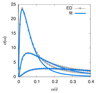
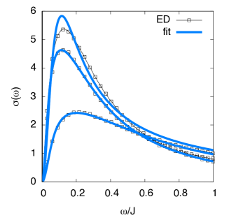
Figure 3: (a) Optical conductivity per particle calculated by ED on a one-dimensional clean chain (no extrinsic site disorder) with thermal inter-molecular disorder in the static limit $1/\tau_{in}=0$ (gray squares). The full blue lines are the corresponding fits with Eq. (II.4). Parameters are $\lambda=0.17$ and $T=0.05;0.1;0.2J$ (from highest to lowest peak); the unit of conductivity is the Mott-Ioffe-Regel value $\sigma_{0}=ne^{2}a^{2}/\hbar$, with $a$ the inter-molecular distance and $n$ the density (see text); frequencies are expressed in units of $J/\hbar$, the inter-molecular transfer rate; (b) Same, with extrinsic site disorder $\Delta=0.2J$ included.

In order to provide a benchmark for its practical use in the analysis of experiments, here we test our formula on the results of exact diagonalization (ED) studies of a model system that has been successfully appliedTroisi06 ; Fratini09 ; Ciuchi11 ; Ciuchi12 to address the microscopic transport mechanism in organic semiconductors. By performing fits of the exactly calculated spectra we are able to check that formula Eq. (II.4) allows to consistently extract the microscopic parameters of the theory, and that it accurately recovers those calculated independently within the model when these are known. It can therefore be used with confidence as a simple and powerful tool for the analysis of experiments.

The modelTroisi06 ; Fratini09 ; Ciuchi11 ; Ciuchi12

$$H=\sum_{i}\epsilon_{i}c^{+}_{i}c_{i}-\sum_{\langle ij\rangle}J_{ij}(c^{+}_{i}c_{j}+H.c.)$$ (15)

considers one-dimensional conduction in the presence of disorder in the inter-molecular transfer integrals $J_{ij}$ (of average $J$), arising due to inter-molecular displacements of thermal origin. Such intrinsic disorder is governed by the temperature $T$, that sets the amplitude of inter-molecular vibrations, and by the dimensionless coupling $\lambda$, that controls how inter-molecular motions affect the electronic states (see e.g. Ref.Ciuchi12 ). Site disorder is also included, representing extrinsic electrical potentials $\epsilon_{i}$ originating from impurities and defects.Ciuchi12 ; Minder14 . The amount of extrinsic disorder is characterized by the variance $\Delta$ of the site energy distribution, that is taken to be Gaussian. The model is solved in the static limit, corresponding to $1/\tau_{in}=0$, where both the $\epsilon_{i}$ and $J_{ij}$ are time-independent variables. As shown in Fig. 2-a this assumption does not change significantly the lineshape in the peak region, and it has the advantage of allowing for an exact solution of the problem, which is done here via exact diagonalization on a 256-site chain and subsequent averaging over a large number of disorder configurations (up to $100000$). Full details on the microscopic model and the method of solution can be found in Ref. Ciuchi12 .

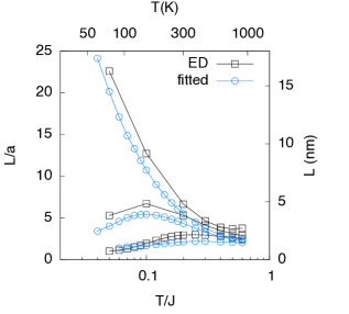
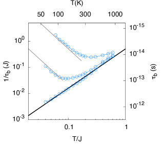
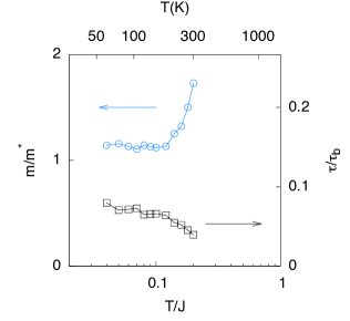
Figure 4: (a) The values of $L$ vs $T$ extracted from the fits (blue circles) are compared with the exact values evaluated via ED (gray squares); from top to bottom $\Delta=0;0.2;0.45J$; the right axis units are obtained assuming $a=7.2\AA$ as appropriate for rubrene; (b) Fitted values of the backscattering rate $1/\tau_{b}$ that controls electron localization (blue circles, from bottom to top $\Delta=0;0.2;0.45J$); black triangles are estimates obtained from the peak position via Eq. (14); the full line is a perturbative estimate valid for the intrinsic case $\Delta=0$ (see text). The left axis is in units of $1/J$, the right axis in $s$, assuming $J=130meV$; (c) inverse effective mass estimated from Eq. (7) (left) and ratio of the scattering timescales (clean limit $\Delta=0$ only).

In Figs. 3-a and 3-b we show representative optical conductivity spectra obtained from ED at different temperatures for intrinsic disorder alone (a), and with added extrinsic disorder (b). The spectra are plotted in units of $\sigma_{0}=ne^{2}a^{2}/\hbar$. In all cases, the optical absorption vanishes at $\omega\to 0$ as expected in a localized system and shows a characteristic peak at a frequency that appears to be ruled by the amount of disorder: the peak in (a) is progressively suppressed and moves to higher frequencies upon increasing the thermal disorder. The peak is located at even higher frequencies in (b) due to the presence of additional extrinsic disorder [note the larger frequency interval in panel (b)]. For sufficiently large disorder/temperature, a fully incoherent regime can be reached where the whole optical absorption lies below the the Mott-Ioffe-Regel value $\sigma_{0}$ (this value is $1$ in the units of Fig. 3).

The full lines are fits to the phenomenological lineshape Eq. (II.4), which satisfactorily reproduce the exact spectra in the relevant region of the localization peak. The localization length $L$ extracted from the fits is shown in Fig. 4-a (blue circles). The extracted values agree quite well with the exact values given in Ref. Ciuchi12 (gray squares). It is important to stress that such exact values were obtained via a sum rule involving the whole optical conductivity spectrum, i.e. the optical response of the electrons at all frequencies [see Eq. (10) in Ref. Ciuchi12 ]. The quantitative agreement between the fitted and exact values implies that the present phenomenological fitting procedure is able to carefully extract the localization length from the knowledge of the optical response in the peak region alone. This is crucial when it comes to the analysis of experimental data, where the spectrum at all frequencies is generally not known and the exact sum rule analysis for the determination of $L$ cannot be applied.

The fitted backscattering rate is shown in Fig. 4-b (blue circles). In the intrinsic regime, the temperature dependence is consistent with $1/\tau_{b}\propto T^{3/2}$. From the results in Fig. 4-b we argue that in the present units the backscattering rate is quantitatively described by $1/\tau_{b}\simeq 3\lambda T^{3/2}/J^{1/2}$, which is shown as a full black line (we have checked that this result holds at different values of $\lambda$). This relation can be used in principle to determine experimentally the value of the electron-vibration coupling $\lambda$ from the value of $\tau_{b}$ fitted on the optical conductivity spectra in sufficiently pure samples. A similar analysis yields $1/\tau_{b}\simeq(0.6\Delta)^{4}/(JT^{2})$ in the extrinsic limit (strong extrinsic disorder, low temperatures, gray lines). We note that use of the simple Eq. (14) to extract the backscattering rate from the position of the peak alone gives results that are consistent with the fits, both in the intrinsic regime ($\Delta=0$) and for weak extrinsic disorder ($\Delta=0.2J$). Deviations arise for large extrinsic disorder and at low temperatures, i.e. where $0.3\hbar/\tau_{b}\gtrsim k_{B}T$, in which case Eq. (13) should be used instead.

Eq. (II.4) also allows to extract the elastic scattering time $\tau$ from the optical conductivity data, provided that the overall disorder is not too large. Fits to the exact results from the microscopic one-dimensional model in the clean limit ($\Delta=0$) yield $1/\tau\simeq 40\lambda T^{3/2}/J^{1/2}$. Comparing this result to the value of $\tau_{b}$ given above, we see that in the present one-dimensional model the elastic and backscattering timescales are related by an approximately constant ratio $\tau/\tau_{b}\simeq 0.07$. This is shown in Fig. 4-c (right axis), and agrees with the Thouless argument given after Eq. (6). We note that when the disorder becomes large, the scattering rate $1/\tau$ becomes comparable with the bandwidth itself and it is no longer possible to extract this parameter with sufficient confidence within the present fitting procedure. This explains why the data of Fig. 4-c are limited to the clean case $\Delta=0$ and to temperatures $T<0.2J$.

Finally, in Fig. 4-c (left axis) we check the validity of Eq. (7) by plotting the estimated band mass $m^{*}$ as obtained from the ratio $L^{2}/[2k_{B}T\tau(\tau_{b}-\tau)]$, by substituting the fitted values of $L,\tau$ and $\tau_{b}$ reported in panels a and b. The estimated band mass is expressed in units of the known band mass of the one-dimensional model, $m=1/2J$. For all temperatures $T\lesssim 0.15J$ we have $m^{*}\simeq m$, while the departure observed at the highest temperatures can again be ascribed to an inaccurate fit of the elastic scattering rate when this becomes comparable to the bandwidth. The agreement of the estimated $m^{*}$ with the known value means that Eq. (7) can be used in practice to estimate the band mass when the localization length $L$ and the scattering timescales are known, or alternatively to estimate $L$ from the known value of the band mass and the fitted values of the scattering timescales.

IV Experimental analysis

IV.1 Rubrene FETs

Few optical absorption experiments on field-effect doped crystalline organic semiconductors have been reported in the literatureFischer ; Li ; Okamoto , all of them performed on rubrene single crystals. Measurements of different groups, all taken at room temperature, are reproduced in Fig. 5. The data have been rescaled here to recover, in the d.c. limit, the mobility values that have been measured independently via the FET transfer characteristics (the reported FET mobility is $\mu=5cm^{2}/Vs$ in Refs. Li ; Fischer and $\mu=4cm^{2}/Vs$ in Ref. Okamoto ). The different optical measurements exhibit considerable scatter, possibly related to differences in the experimental setups. However, all of them show (or are compatible with) an absorption peak around $\omega\simeq 50meV$, which can not be possibly reproduced within the semiclassical Drude model. We argue that this feature is a fingerprint of the transient localization mechanism.

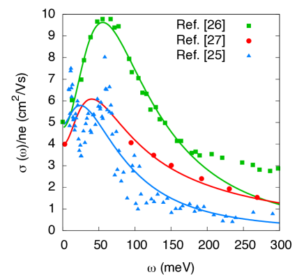
Figure 5: Available optical absorption data on rubrene FETs. The data are expressed in mobility units and have been rescaled to yield the FET mobility value in the zero frequency limit (see text). Full lines are fits of the data via Eq. (II.4).

We focus first on the data of Ref. Li measured in the direction of highest conduction and at the highest reported gate voltage. As illustrated in Fig. 5, the analytical formula Eq. (II.4) is able to closely reproduce the experimental absorption peak at $\omega\simeq 50meV$. The following parameters are obtained from the fitting procedure: $1/\tau_{in}=13meV$, $1/\tau_{b}=40meV$, $1/\tau=195meV$. The extracted inelastic scattering rate $1/\tau_{in}$ is consistent with the frequency of the intermolecular vibrations in rubrene, $\omega_{0}=5-15meV$, as independently measured and theoretically calculated in Refs. Ren ; Girlando . On the other hand, since there are no independent measurements of the backscattering rate available on the present device, we compare the extracted value $1/\tau_{b}=40meV$ with the results of the microscopic model calculation reported in Fig. 4-b. Taking $J=130$meV as representative for rubrene implies $(1/\tau_{b})/J=40/130=0.3$. It can be read from Fig. 4-b that this value at room temperature ($T/J=0.2$) corresponds to a degree of extrinsic disorder $\Delta\simeq 0.45J=60$meV, which is in the typical range observed in these devices. The extracted value of $\Delta=60$meV implies that carrier transport in the studied sample is still far from the intrinsic regime. This conclusion agrees with the fact that the measured FET mobility $\mu=5cm^{2}/Vs$ is considerably lower than the highest values $>20cm^{2}/Vs$ reported in rubrene-based FETs of higher purity Podzorov ; Takeya

We note that in Eq. (II.4) the global amplitude is proportional to the factor $nL^{2}$, so that fits to the optical conductivity do not give access separately to the carrier density $n$ and the localization length $L$. In clear, the localization length can only be obtained if $n$ is known independently from an independent measurement or, alternatively, if it can be estimated from the known value of the band mass (following the procedure described in Appendix A). In the FET geometry used in Ref Li , for example, the carrier density was determined from the known device capacitance to $n=3.7\cdot 10^{12}$cm^-2, which allows us to determine $L/a=1.9$ from the fit in Fig. 5. This value is actually in very good agreement with the value predicted from the microscopic model at this temperature and this level of extrinsic disorder, $L/a=2.1$, as shown in Fig. 4-a.

Tentative fits to the other available measurements can be attempted for qualitative purposes, even though it is more difficult to extract reliable quantitative parameters in these cases. To reduce the number of degrees of freedom in the fits we fix the value of the inelastic scattering rate to $1/\tau_{in}=13meV$ as obtained previously, which is justified because the inter-molecular vibration frequencies are not expected to vary from sample to sample. The data of Ref. Fischer exhibit considerable scatter, and the fit quality is not as good as in the previous case. A localization peak is well visible at $\omega\simeq 50$meV as in the data of Ref. Li , but the large increase of conductivity at low frequency leads to a two-peak structure that cannot be well described by our formula (the resulting peak position in the fit lies in between the two maxima in the experimental data). Finally in Ref. Okamoto only the high frequency tail of the absorption was measured, but not the region of the localization peak that is of interest to us. Still, our fit with Eq. (II.4) does reveal the existence of a localization peak in the region where no data points are available, which provides an alternative interpretation to the one proposed in Ref. Okamoto based on the semiclassical Drude model.

V Concluding remarks

We have derived a general phenomenological formula that describes the low-frequency optical absorption of charge carriers in disordered systems, interpolating between the Drude-like response of diffusive carriers and the finite-frequency peak shape expected in the presence of Anderson localization. Such Drude-Anderson formula provides a useful alternative to the standard Drude model and to its known generalizations — extended Drude, Drude-Lorentz or Drude-SmithSmith models (see e.g. Ref. Ulbricht-RMP11 ) — for the analysis of optical conductivity experiments. This analytical formula has been benchmarked by comparing it with exact numerical results obtained on a microscopic model with on-site and inter-site disorder that is believed to be relevant to high-mobility organic semiconductors, and has been shown to give a physically transparent description of the phenomenon of transient localization. We have then applied it to the analysis of the available experimental data in rubrene-based FETs, showing that these can be consistently and quantitatively interpreted within the transient localization scenario.

Interestingly, the same concept of transient localization that has been developed in recent years in the context of organic semiconductors was also applied in the past to low-dimensional organic metals such as the TCNQ salts Shante78 ; Gogolin75 ; Madhukar77 ; Gogolin82 . Such compounds have a molecular structure very similar to the organic semiconductors studied here, consisting of organic molecules weakly bound by van der Waals forces. Similar microscopic mechanisms are therefore expected to be at work, and it is not surprising that conductive properties comparable to those of crystalline organic semiconductors are commonly observed in organic metals, at least in the high temperature range where electronic correlations are unimportant. Indeed, the d.c. conductivities in these materials typically exhibit a power law decrease with temperature, and room temperature mobilities in the range $\mu=0.1-10cm^{2}/Vs$ can be deduced from the reported conductivity values at room temperature (these are on the order of $\sigma=10-1000(\Omega cm)^{-1}$, see Ref. Graja for a complete review of different compounds).

More recently, it has been independently suggested based on a combined analysis of the d.c. and optical conductivity Gunnarsson that the modest conductivity values observed Takenaka in the two-dimensional organic superconductor $\theta$-ET₂I₃ [$\sigma=10(\Omega cm)^{-1}$ at room temperature, again below the Mott-Ioffe-Regel limit] originate from the coupling of electrons to molecular vibrations. Our theory does provide support to this scenario, since both the lineshapes and temperature evolution of the optical absorption spectra of Ref. Takenaka are comparable to those of our Fig. 3-a. The comparison can be made even more quantitative by fitting the data reported in Ref. Takenaka . For this we use the generalization of the optical conductivity formula Eq. (11) that applies to metallic systems in the degenerate limit, presented in Appendix C. The extracted backscattering rate $1/\tau_{b}\simeq 14meV$ ($\tau_{b}\simeq 3.1\cdot 10^{-13}s$) at room temperature is right in range expected from electron-molecular vibration coupling (cf. Fig. 4-b). The similarities observed in the transport and optical properties of organic semiconductors, conductors and superconductors suggest that the transient localization scenario discussed here is a more general and common characteristic of the whole broad class of organic molecular crystals.

Finally, we mention that in a different class of low-dimensional materials — carbon nanotubes — an ubiquitous optical absorption peak has been reported by several groups in the far infrared range Kampfrath ; Ichida ; Ulbricht-RMP11 , whose microscopic origin could possibly be related to the localization phenomena described in this work.

Appendix A High frequency limit: semiclassical dynamics

The semiclassical diffusion of electrons corresponds to the assumption that velocity correlations are destroyed after a relaxation time $\tau$. This assumption is appropriate when the particles are only weakly scattered by disorder. To illustrate this we take the simple model:

$$C(t)=C(0)e^{-t/\tau}$$ (16)

$$\Delta X^{2}(t)=C(0)\tau\left[t-\tau+\tau(1-e^{-t/\tau})\right].$$ (17)

Eq. (18) assumes that correlations in the absence of scattering are independent of time, which is certainly valid for classical trajectories. The particle spread Eq. (17) has been obtained by double integration of the correlation function over time. Both quantities are illustrated in Fig. 1 as dashed lines. Eq. (17) describes an initial ballistic behavior $\Delta X^{2}(t)=C(0)t^{2}/2$ followed by diffusion $\Delta X^{2}(t)=C(0)\tau t$ (the corresponding diffusivity is $D=C(0)\tau/2$). Performing the Fourier transform yields $C(\omega)=C(0)/(1/\tau-i\omega)$ and the corresponding optical absorption is obtained via Eq. (3). We note that this derivation recovers the usual Drude response in the high temperature limit: in this case we have $C(0)=2\langle V^{2}\rangle=2Nk_{B}T/m^{*}$ from the equipartition principle, and expanding Eq. (3) for $k_{B}T\gg\hbar\omega$ we have

$$\sigma(\omega)=(ne^{2}\tau/m^{*})Re\left[\frac{1}{1-i\omega\tau}\right].$$ (18)

The Drude expression Eq. (18) correctly describes the optical response of the complete model Eq. (II.4) in the high frequency limit where $\omega\gg 1/\tau_{in},1/\tau_{b}$, as shown in Fig. 2. In this case the second term between brackets in Eq. (10) is negligible and the first term is precisely of the Drude form with the correct prefactor. This can be easily demonstrated by observing that $\tanh(\hbar\omega/2k_{B}T)/\hbar\omega=1/2k_{B}T$ at high temperatures and using the relation $L^{2}=D_{sc}\tau_{b}$ [see Eq. (6)] with $D_{sc}=2\langle V^{2}\rangle\tau=2k_{B}T\tau/m^{*}$, which yields Eq. (7).

More generally, the knowledge of the semiclassical diffusivity is extremely useful when it comes to analyzing experimental data where the absolute number of carriers is not known, because it provides a prescription to to estimate the carrier number provided that the effective mass $m^{*}$ is known. This is a non-trivial issue, as fits of the optical conductivity via Eq. (II.4), which is proportional to the product $nL^{2}$, cannot in principle extract $n$ and $L$ separately. In practice, to extract $n$ one replaces $L^{2}$ in Eq. (II.4) by its expression Eq. (7), so that the prefactor of the optical conductivity now only depends on $n$ via the known values of $m^{*}$ and $\tau$.

A generalization of Eq. (18) that recovers the usual Drude formula in the degenerate limit at $T=0$ is reported in Appendix C and can be found in Refs. Mayou00 ; Gruner .

Appendix B Quantum diffusion in the phenomenological model

We provide here the full expression for the quantum diffusion in the phenomenological model Eq. (8):

$$\Delta X^{2}_{RTA}(t)=2NDt+$$ (19)

$$+\frac{NL^{2}}{\tau_{b}-\tau}\left[\frac{(1-e^{-\tilde{\gamma}_{b}t})}{\tau_{b}\tilde{\gamma}_{b}^{2}}-\frac{(1-e^{-\tilde{\gamma}t})}{\tau\tilde{\gamma}^{2}}\right]$$

where we have defined the quantities $\tilde{\gamma}=(1/\tau+1/\tau_{in})$ and $\tilde{\gamma}_{b}=(1/\tau_{b}+1/\tau_{in})$, and

$$D=\frac{1}{(1+\tau/\tau_{in})(1+\tau_{b}/\tau_{in})}\frac{L^{2}}{2\tau_{in}}$$ (20)

is the diffusion constant at long times. Eq. (9) of the main text is obtained by taking the limit of slow disorder fluctuations, $\tau_{in}\gg\tau_{b},\tau$.

The above expression allows us to define the transient localization length as

$$L^{2}(\tau_{in})=\frac{L^{2}}{(1+\tau/\tau_{in})(1+\tau_{b}/\tau_{in})}$$ (21)

so that $D=L^{2}(\tau_{in})/2\tau_{in}$. The quantity in Eq. (21) is the spread of the localized electron wavefunction on a timescale $\tau_{in}<\infty$, as defined in Eq. (7) of Ref. Ciuchi12 . It is clear from the above definition that $L(\tau_{in})<L$ for all finite $\tau_{in}$. In practical cases when the timescales $\tau_{in},\tau_{b}$ and $\tau$ are not well separated, this can make a sizable correction to the mobility and the full expression Eq. (21) should be used in Eqs. (9) and (10) instead of the bare $L$.

Appendix C Case of a degenerate electron system

As explained in the main text the real part of the optical conductivity is obtained as

$$\sigma(\omega)=\frac{e^{2}\tanh(\frac{\hbar\omega}{2k_{B}T})}{\hbar\omega\Omega}ReC_{+}(\omega),$$ (22)

where $e$ is the electron charge, $\Omega$ is the system volume and $C_{+}(\omega)=\int_{0}^{\infty}e^{i\omega t}C_{+}(t)dt$. $C_{+}(t)$ is the time-dependent velocity correlation function for the N-electron system. When the electron system is non degenerate and follows the Maxwell-Boltzmann distribution the velocity correlation $C_{+}$ has a simple expression in terms of the velocity correlation of a single particle, being N-times the thermodynamical average of the velocity correlation function of one electron alone. The approach developed in the main text is based on the assumption that the velocity correlation for one electron can be well represented by Eqs. (4) and (5).

In the case of a degenerate electron system the many-body velocity correlation function is no longer equal to N times the thermodynamical average of the correlation function of one electron alone, due to quantum statistics. Yet at low temperature and low frequency $k_{B}T\ll\hbar\omega\ll E_{F}$, where $E_{F}$ is the Fermi energy, it is possible to express the conductivity in terms of the velocity correlation function $C_{+}(E_{F},t)$ for states at $E_{F}$. The derivation can be found in Refs. Mayou00 ; Gruner . At frequencies much smaller than the Fermi energy the conductivity is then given by:

$$\sigma(E_{F},\omega)=e^{2}N(E_{F})\ Re\int_{0}^{\infty}e^{i\omega t}C_{+}(E_{F},t)dt$$ (23)

The above equation is similar to Eq. (22) except that $C_{+}(t)$ is replaced by $C_{+}(E_{F},t)$, and the prefactor now involves $N(E_{F})$, the density of states per unit volume and spin at the Fermi energy (a perfect spin degeneracy is assumed here). For the velocity correlation at the Fermi energy we assume that the behavior is analogous to that given in Eq. (4) in the main text, i.e.:

$$C(E_{F},t) = \frac{C(E_{F},0)}{1/\tau-1/\tau_{b}}\left[\frac{1}{\tau}e^{-t/\tau}-\frac{1}{\tau_{b}}e^{-t/\tau_{b}}\right]$$ (24)

$$\Delta X^{2}(E_{F},t) = \frac{C(E_{F},0)}{1/\tau-1/\tau_{b}}$$

$$\times\left[\tau_{b}(1-e^{-t/\tau_{b}})-\tau(1-e^{-t/\tau})\right]$$

The velocity correlation at zero time $C(E_{F},0)$ is typically given by $2V_{F}^{2}/d$ where $V_{F}$ is the Fermi velocity and $d$ the dimensionality. The above Eq. (C) describes the localization of electrons at the Fermi energy in a way similar to that described in the main text for non-degenerate electrons.

The effect of inelastic scattering can be introduced in the spirit of the RTA as in Eq. (8) of the main text:

$$C_{RTA}(E_{F},t)=C_{+}(E_{F},t)e^{-t/\tau_{in}}.$$ (26)

This leads to the following expression for the complex conductivity:

$$\sigma(E_{F},\omega) = e^{2}N(E_{F})\frac{C(E_{F},0)}{1/\tau-1/\tau_{b}}$$

$$\times\left[\frac{1}{1+\tau/\tau_{in}-i\omega\tau}-\frac{1}{1+\tau_{b}/\tau_{in}-i\omega\tau_{b}}\right]$$

Except for the different prefactor, this expression is analogous to Eq. (II.4) given in the main text and can therefore describe a finite frequency localization peak. When the inelastic scattering time $\tau_{in}$ tends to infinity then the zero frequency conductivity vanishes. When the inelastic scattering time is finite the zero frequency conductivity is finite and varies proportionally to $1/\tau_{in}$ in agreement with the Thouless regime, as discussed in the main text. The usual Drude formula is recovered in the limit $\tau_{b}\to\infty$.

- (1) A. Troisi & G. Orlandi, Phys. Rev. Lett. 96, 086601 (2006).
- (2) J.-D. Picon, M. N. Bussac, and L. Zuppiroli, Phys. Rev. B 75, 235106 (2007).
- (3) S. Ciuchi, S. Fratini and D. Mayou, Phys. Rev. B 83, 081202(R) (2011).
- (4) L. Friedman, Phys. Rev. 140, A1649 (1965).
- (5) Y. C. Cheng et al., J. Chem. Phys. 118, 3764 (2003).
- (6) S. Fratini and S. Ciuchi, Phys. Rev. Lett. 103, 266601 (2009).
- (7) V. Cataudella, G. De Filippis, and C. A. Perroni, Phys. Rev. B 83, 165203 (2011).
- (8) S. Ciuchi and S. Fratini, Phys. Rev. B 86, 245201 (2012)
- (9) D. Mayou, Europhys. Lett. 6, 549 (1988).
- (10) D. Mayou and S. N. Khanna, J. Phys. I (France) 5, 1199 (1995).
- (11) S. Roche and D. Mayou, Phys. Rev. B 60, 322 (1999).
- (12) D. Mayou, Phys. Rev. Lett. 85, 1290 (2000).
- (13) F. Triozon, J. Vidal, R. Mosseri, and D. Mayou, Phys. Rev. B 65, 220202 (2002).
- (14) G. Trambly de Laissardière, J.-P. Julien, and D. Mayou, Phys. Rev. Lett. 97, 026601 (2006).
- (15) G. Trambly de Laissardière and D. Mayou, Phys. Rev. Lett. 111, 146601 (2013)
- (16) N. H. Lindner and A. Auerbach, Phys. Rev. B 81, 054512 (2010)
- (17) M. Dressel and George Grüner ”Electrodynamics of Solids: optical properties of electrons in matter”, Cambridge University Press, (2002).
- (18) Electron localization, embodied in the condition , has a direct geometrical interpretation that can be read directly from Fig. 1-b: because the long-time diffusivity is proportional to the integral of the velocity correlation function, in a localized system the positive area under the curve is exactly compensated by the negative backscattering part. This cancellation is destroyed by the exponential decay in Eq. (8), restoring a finite diffusivity at long times.
- (19) The value of the initial constant is also fixed by the model to . We point out here that this value does not correspond to the actual short-time limit of the correlation function, . This discrepancy arises from the fact that the simple model Eq. (4) is devised to provide a good description of the carrier dynamics at frequencies relevant for diffusion and localization (intermediate and long times), but it has no information on the high frequency behavior related to the exact form of the electronic bands (short times). Strictly speaking, Eq. (4) holds at times with a time of the order of the intermolecular transfer time .
- (20) C.W.J. Beenakker, Rev. Mod. Phys. 69, 731 (1997)
- (21) N. F. Mott, and M. Kaveh Adv. Phys. 34, 329 (1985)
- (22) N. V. Smith, Phys. Rev. B, 64, 155106
- (23) O. Gunnarsson and K. Vafayi, Phys. Rev. Lett. 98, 219802 (2007)
- (24) N. A. Minder, S. Lu, S. Fratini, S. Ciuchi, A. Facchetti, A. F. Morpurgo, Adv. Mat., 26, 1254 (2014)
- (25) M. Fischer, M. Dressel, B. Gompf, A.K. Tripathi, and J. Pflaum, Appl. Phys. Lett. 89, 182103 (2006).
- (26) Z. Q. Li, V. Podzorov, N. Sai, M. C. Martin, M. E. Gershenson, M. DiVentra, and D. N. Basov, Phys. Rev. Lett. 99, 016403 (2007).
- (27) R. Uchida, H. Yada, M. Makino, Y. Matsui, K. Miwa, T. Uemura, J. Takeya, and H. Okamoto, Appl. Phys. Lett. 102, 093301 (2013)
- (28) Z. Q. Ren, L. E. McNeil, S. Liu, and C. Kloc, Phys. Rev. B 80, 245211 (2009).
- (29) A. Girlando, L. Grisanti, M. Masino, I. Bilotti, A. Brillante, R. G. DellaValle, and E. Venuti, Phys. Rev. B 82, 035208 (2010).
- (30) V. Podzorov, E. Menard, J. A. Rogers, M. E. Gershenson, Phys. Rev. Lett. 95, 226601 (2005).
- (31) T. Hasegawa and J. Takeya, Sci. Technol. Adv. Mater. 10, 024314 (2009)
- (32) R. Ulbricht, E. Hendry, J. Shan, T. F. Heinz, and M. Bonn Rev. Mod. Phys. 83, 543 (2011)
- (33) V. K. S. Shante, J. Phys. C: Sol. Stat. Phys., 11, (1978).
- (34) A. A. Gogolin, S. P. Zolotukhin, V. I. Mel’nikov, E. I. Rashba, I. F. Shchegolev, JETP Lett., 22, 1, (1975)
- (35) A. Madhukar and M. H. Cohen, Phys. Rev. Lett. 38, 76 (1977).
- (36) A. A. Gogolin Phys. Rep. 86, 1, (1982).
- (37) A. Graja, ”Low-dimensional organic conductors” World Scientific, (1992).
- (38) K. Takenaka et al., Phys. Rev. Lett. 95, 227801 (2005).
- (39) T. Kampfrath, K. von Volkmann, C.M. Aguirre, P. Desjardins, R. Martel, M. Krenz, C. Frischkorn, M. Wolf and L. Perfetti, Phys. Rev. Lett. 101 267403 (2008)
- (40) M. Ichida, S. Saito, T. Nakano, Y. Feng, Y. Miyata, K. Yanagi, H. Kataura, H. Ando, Solid State Comm. 151 1696 (2011)