Destruction of Anderson localization by nonlinearity in kicked rotator at different effective dimensions

Abstract

We study numerically the frequency modulated kicked nonlinear rotator with effective dimension $d=1,2,3,4$. We follow the time evolution of the model up to $10^{9}$ kicks and determine the exponent $\alpha$ of subdiffusive spreading which changes from $0.35$ to $0.5$ when the dimension changes from $d=1$ to $4$. All results are obtained in a regime of relatively strong Anderson localization well below the Anderson transition point existing for $d=3,4$. We explain that this variation of the exponent is different from the usual $d-$dimensional Anderson models with local nonlinearity where $\alpha$ drops with increasing $d$. We also argue that the renormalization arguments proposed by Cherroret N et al. arXiv:1401.1038 are not valid.

Dated: March 11, 2014

1 Introduction

At present there is a significant interest to effects of nonlinearity on Anderson localization [1]. The early theoretical and numerical studies [2, 3] have been followed by more recent and more detailed analysis performed by different groups [4, 5, 6, 7, 8, 9], [10, 11, 12, 13, 14, 15]. The interest to this problem comes also from the side of mathematics which puts forward a fundamental question on how the pure point spectrum of Anderson localization is affected by a weak nonlinearity [16, 17, 18]. At the same time the experiments on spreading of light in nonlinear photonic lattices [19, 20] and of Bose-Einstein condensates of cold atoms in disordered potential [21] start to be able to observe effects of nonlinearity on localization.

The main effect found in numerical simulations is a subdiffusive spreading of wave packet over lattice sites induced by a moderate nonlinearity. Large time scale simulations are required to determine the spreading exponent with a good accuracy and hence the choice of a good model, which is easy for numerical simulations and at the same time captures the main physical effects, is important. One of such models is the model of kicked nonlinear rotator [2], where nonlinear phase shifts are introduced in the quantum Chirikov standard map, known also as the kicked rotator [22].

It is also important that the kicked rotator has one more interesting extension: the frequency modulated kicked rotator (FMKR) introduced in [23]. In this model the kick amplitudes are modulated with $d-1$ incommensurate frequencies that allows to model the Anderson transition in effective dimensions $d=3,4$ [24, 25, 26]. This FMKR model, proposed theoretically, has been realized in skillful and impressive experiments with cold atoms by Garreau group [27]. These experiments allowed to observe the Anderson transition in $d=3$ and to determine experimentally the critical exponents which have been found to be in agreement with analytical and numerical calculations [28]. At the moment the Garreau experiments are definitely represent the most advanced experimental investigation of the Anderson transition both in fields of cold atoms and solid state disordered systems.

In a recent preprint [29] it is proposed to to study frequency modulated kicked nonlinear rotator (FMKNR) model. It is argued there that the FMKNR allows to investigate the effects of nonlinearity of Anderson transition in $d=3$. Here, we show that the renormalization group analysis performed in [29] is not relevant for the main physical effects leading to the nonlinearity induced wave spreading. However, the investigation the FMKNR model itself is interesting and provides some new information on effects of nonlinearity on Anderson localization. Thus we present here the results of our numerical studies of FMKNR in effective dimensions $d=1,2,3,4$ up to times $t=10^{9}$. The model is described in Sec.2, numerical results are presented in Sec.3, simple estimates are presented in Sec.4 and discussion is given in Sec.5.

2 FMKNR model description

The time evolution of the wave function of the FMKNR is described by the equation

$$\psi(t+1)=e^{-i(\hat{H}_{0}+\hat{H}_{nl})}e^{-i\hat{V}(t)}\psi(t)\;,$$ (1)

where

$$\hat{H}_{0}(n)=\xi_{n}\;\;(model\;M1)\;;\;\;\;\hat{H}_{0}(n)=Tn(n+\zeta)/2\;\;(model\;M2)\;,$$ (2)

with $\xi_{n}$ being random energies distributed homogeneously in the interval $-\pi,\pi$ (model $M1$) and $H_{0}(n)=Tn(n+\zeta)/2$ (model $M2$) are rotational phases in a kicked rotator with $\zeta$ corresponding to a quasi-momentum of Bloch waves in kicked optical lattices and parameter $T\sim\hbar_{eff}\sim 1$. Here, $n$ is a quantum number corresponding to momentum quantization [23, 24, 25, 26, 27, 28]. This part of Hamiltonian describes a free propagation.

• 

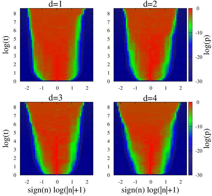
Figure 1: (Color online) Time evolution of the probability spreading $p=|\psi(n)|^{2}$, shown by color, over momentum levels $n$ for the model $M1$ at $k=1.5$ ($d=1$); $k=0.5,\epsilon=0.75$ ($d=2,3,4$), and $\beta=1$, the time interval is $1\leq t\leq 10^{9}$. Initial state is $n=0$. Probability $p$ is shown by color variation given by color bars. The logarithms are decimal.

The nonlinear phase shift, as in [2], is given by

$$\hat{H}_{nl}=\beta|\psi(n)|^{2}\;,$$ (3)

where $\beta$ is the strength on nonlinear interactions and $\psi(n)$ is taken in the momentum representation. The norm $\sum_{n}|\psi(n)|^{2}=1$ is conserved by unitary evolution.

The part with the kick is written in the phase representation for $\psi(\theta)$ which is conjugated to the momentum representation ($\psi(\theta+2\pi)=\psi(\theta)$, ${\hat{n}}=-i\partial/\partial\theta$):

$$V(\theta,t)=k\cos\theta[1+\epsilon\Pi_{i=1}^{d-1}\cos(\omega_{i}t)]\;.$$ (4)

Here, $\epsilon$ represents a strength of frequency modulation with $d-1$ incommensurate frequencies $\omega_{i}$ and $t$ is measured in a number of map iterations. For $d=1$ in $M2$ case we obtain the usual kicked rotator [22] with $k\sim 1/\hbar_{eff}$, $T\sim\hbar_{eff}$ and the chaos parameter $K=kT=const$ ($\hbar_{eff}$ is an effective Planck constant). For $d=2$ we use $\omega_{1}=2\pi/\lambda$, for $d=3$ we use $\omega_{1}=2\pi/\lambda$, $\omega_{2}=2\pi/\lambda^{2}$. For $d=4$ we add frequency $\omega_{3}=2\pi/\sqrt{2}$. Here $\lambda=1.32471795724475$ is a root of cubic equation [25]. At $\beta=0$ the models $M1$ and $M2$ manifest the phenomenon of Anderson localization in effective dimensions $d=1,2,3,4$; for $d=3,4$ there is the Anderson transition for $k>k_{c}$ at a certain fixed $\epsilon$ [25, 26, 27, 28]. For $d=3$ the curve of the Anderson transition in the plane $(k,\epsilon)$ is analyzed in [30].

For $\beta\sim 1$ the model $M1$ at $d=1$ (KNR) shows a subdiffusive spreading of wave packet over sites (levels) with the second moment growth characterized by an exponent $\alpha\sim 0.4$ [2]:

$$\sigma=\sum_{n}|\psi(n)|^{2}n^{2}=<n^{2}>\sim t^{\alpha}.$$ (5)

It was argued [2] that this model effectively describes the spreading in discrete Anderson nonlinear Schrödinger equation (DANSE). The later studies indeed confirmed that in DANSE the exponent $\alpha$ is approximately the same as in the KNR [4, 7, 9]. The examples of probability spreading in the FMKNR at $d=1,2,3,4$ in the model $M1$ are shown in Fig. 1.

The study of the FMKNR at $d=3$ has been proposed in [29]. At $\beta=0$ the model FMKR can be exactly mapped on an Anderson model in effective dimension $d$ [24, 25] by a transformation similar to those used in $d=1$ case [31, 32]. Indeed, since the phases $\theta_{i}=\omega_{i}t$ rotates with fixed frequencies we can write the Hamiltonian in effective extended dimension $d$:

$$H(n,n_{i},\theta,\theta_{i})=H_{0}(n)+\sum_{i=1}^{d-1}\omega_{i}n_{i}+\beta\sum_{n_{i}=-\infty}^{\infty}|\psi(n,n_{i})|^{2}+V(\theta,\theta_{i})\delta_{1}(t)$$ (6)

where $\delta_{1}(t)$ is a periodic delta-function with period unity, $n,\theta$ and $n_{i},\theta_{i}(i=1,..,d-1)$ are conjugated pairs of variables. Then the evolution is given by the unitary propagator:

$$\psi(n,n_{i},t+1)=\exp(-iH_{int}(n,n_{i}))\exp(-iV(\theta,\theta_{i}))\psi(n,n_{i},t)\;,$$ (7)

where $H_{int}(n,n_{i})=H_{0}(n)+\sum_{i=1}^{d-1}\omega_{i}n_{i}+\beta\sum_{n_{i}=-\infty}^{\infty}|\psi(n,n_{i})|^{2}$. It is important here that the nonlinear term with $\beta$ contains a sum over all additional effective dimensions $d-1$. In a certain sense this corresponds to long-range interaction of planes in $d-1$ dimensions. This corresponds to the physics of the FMKNR model where nonlinear coupling acts only in $n$ independently of phases $\theta_{i}=\omega_{i}t$.

If we would model a real nonlinear interaction term in dimension $d$ we would have another Hamiltonian

$$H(n,n_{i},\theta,\theta_{i})=H_{0}(n)+\sum_{i=1}^{d-1}\omega_{i}n_{i}+\beta|\psi(n,n_{i})|^{2}+V(\theta,\theta_{i})\delta_{1}(t)$$ (8)

where nonlinear term $\beta|\psi(n,n_{i})|^{2}$ have no summation over $n_{i}$. Then the evolution of $\psi$ is still given by the propagator (7) but with $H_{int}(n,n_{i})=H_{0}(n)+\sum_{i=1}^{d-1}\omega_{i}n_{i}+\beta|\psi(n,n_{i})|^{2}$. Such a local term appears in DANSE in $d=2$ and has been studied in [7]. The numerical results of [7] show that the exponent $\alpha$ of the second moment $n^{2}\propto t^{\alpha}$ decreases when we increase $d$ from $d=1$ to $d=2$ going from $\alpha\sim 0.4$ down to $\alpha\sim 0.25$. The analytical arguments of [7] give:

$$\alpha=2/(3d+2)\;.$$ (9)

Of course, this expression assumes local nonlinear interaction term as in (8) that is rather different from the case of long interactions in effective dimensions effectively appearing in the FMKNR of (1), (6).

All renormalization group arguments presented in [29] are developed for the case of local nonlinear term (8) while the numerical simulations are done for the FMKNR case (1) and (6) corresponding to the long-range interactions. Due to such a mixing of concepts the arguments of [29] are not valid. Also, we point our that the renormalization group arguments [29] assume a proximity to a critical point of the Anderson transition. But all the studies of the nonlinearity induced destruction of Anderson localization show that it takes place even in a relatively strong localization regime and also in $d=1,2$ where the Anderson transition is absent and linear waves are always localized. Due to that reasons we argue that the approach of [29] is not valid for the physics of phenomenon of DANSE. However, the investigation of the FMKNR model at certain $d$ is interesting and thus we present our results below for $d=1,2,3,4$.

3 Numerical results

In our numerical studies we fix $k=1.5$ for $d=1$ and $k=0.5$, $\epsilon=0.75$ for $d=2,3,4$ for both models $M1$ and $M2$ The frequencies $\omega_{i}$ are fixed at values given in the previous Section. For the model $M2$ we use $T=2.89$ as in experiments [29]; we use up to $10$ random values of quasi-momentum $\zeta$ in model $M2$ $(0\leq\zeta<1$) and up to $10$ disorder realizations in model $M1$. The initial state is taken at $n=0$. The transition between momentum and angle representations is done by the fast Fourier transform.

• 

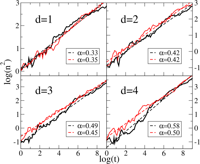
Figure 2: (Color online) Dependence of the second moment $\sigma\equiv\langle n^{2}\rangle$ of probability distribution on time $t$ shown in logarithmic scale for models $M1$ (black) and $M2$ (red) with dimensions $d=1,2,3,4$. Parameters $k,\epsilon,\beta$ are as in Fig. 1 and $T=2.89$ for $M2$. The power law fit of subdifussive spreading $\sigma\sim t^{\alpha}$ is shown by the straight dashed lines for each model. Effective dimensions $d$ and fitted values of $\alpha$ are shown in each panel, logarithms are decimal.

For $d=3,4$ we find that both models have approximately the same critical value $k_{c}$ of Anderson transition. For $d=3$ we have $k_{c}\approx 1.8$ in agreement with [25, 26]. Also for $d=4$ both models have the same critical point $k_{c}\approx 1.15$ at $\epsilon=0.9$ and $k_{c}\approx 1.3$ at $\epsilon=0.75$. At $d-1$ frequencies the classical chaos border becomes very small in $k$ so that random rotational phases in model $M1$ have the Anderson transition approximately at the same point as in the model $M2$. We stress that all amplitudes of $k$ used in our simulations are located in a well localized phase being rather far from the Anderson transition in $d=3,4$. At that $k$ values the localization length $\ell\sim 1-2$ captures only a couple of sites (see Figs.1,9 in [25]).

The spearing of probability $p_{n}=|\psi(n)|^{2}$ over momentum modes $n$ is shown as a function of time $t\leq 10^{9}$ in Fig. 1 for model $M1$. The data show that $|\psi(n)|^{2}$ spreads more or less homogeneously over a plateau (chapeau) which width increases with time.

The growth of the second moment $\sigma$ with time $t\leq 10^{9}$ is shown in Fig. 2 for models $M1$ and $M2$ for a one disorder realization in $M1$ and one value of quasi-momentum in model $M2$ (a random value in the interval $0\leq\zeta<1$).

• 

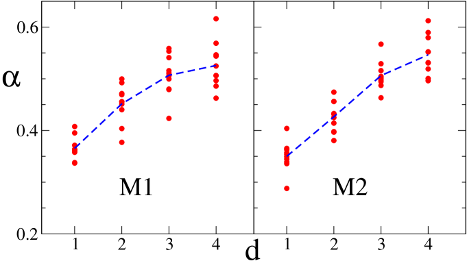
Figure 3: (Color online) The subdifussive spreading exponent $\alpha$ for dimensions $d=1,2,3,4$ of both models. The model parameters are as in Figs. 1, 2. The exponents $\alpha$ are computed up to time $t=10^{8}$ for $10$ random realizations of disorder in model $M1$ and $10$ random values of quasi-momentum $\zeta$ in model $M2$ (left and right panels respectively). Dashed blue curves represent average $\alpha$ dependence on dimension $d$ for each model.

We also determine the dependence $\sigma(t)$ for $1\leq t\leq 10^{8}$ for both models for $10$ realizations of disorder ($M1$) or $10$ random values of $\zeta$ ($M2$). The values of exponent $\alpha$ are shown in Fig. 3 for all four dimensions $d$. Averaging over these 10 values of $\alpha$ we find the average $\alpha$ value and its error-bar. For model $M1$ we obtain $\alpha=0.36\pm 0.02$, $0.45\pm 0.03$, $0.50\pm 0.04$, $0.52\pm 0.04$ and for model $M2$ we obtain $\alpha=0.35\pm 0.03$, $0.43\pm 0.03$, $0.51\pm 0.03$, $0.54\pm 0.04$ respectively for $d=1,2,3,4$. Within the error-bars both models have the same value of $\alpha$ for a given dimension.

We note that the case $d=3$ for model $M2$ has been studied in [29] with numerically obtained value $\alpha\approx 0.4$. However, the time scales considered there are about 1000 times smaller than those considered here. Also in [29] the working point was placed rather close to the Anderson transition so that the localization length of linear problem was rather large so that it was more difficult to reach the asymptotic regime (in our case we are far from the Anderson transition point and $\ell\sim 1-2$).

Our data show a clear tendency of growth of $\alpha$ with $d$ in the FMKNR model (1). Of course, this dependence is absolutely different from the one of (9) obtained for a local nonlinear term.

4 Simple estimates

It is interesting to note that the exponent $\alpha=1/2$ corresponds to a so-called regime of “strong chaos” [9, 10, 33]. Indeed, the numerical simulations performed in [9, 10] introduced a randomization of phases of linear eigenmodes after a fixed time scale $\tau\sim 1$ showing numerically that in such a case $\alpha=1/2$. This relation can be understood on a basis of simple estimates in a following way: the equations of amplitudes of linear modes $C_{m}$ in the interaction representation have a form $i\partial C/\partial t\sim\beta C^{3}$ [2, 4, 7]. In [2, 4, 7] it was assumed that there is a plateau in amplitudes of $C\sim 1/(\Delta n)^{1/2}$ with $|m|<\Delta n$ and $C=0$ outside of the plateau. Then the time scale $t_{s}$ after which a next level outside of plateau will be populated is estimated as $\Gamma\sim 1/t_{s}\sim\beta^{2}C^{6}\sim\beta^{2}/(\Delta n)^{3}$ due to norm conservation. Since the diffusion coefficient is $D\sim(\Delta n)^{2}/t\sim\Gamma$ this gives $\alpha=2/5$ for ($d=1$) and the relation (9) for any $d$ [2, 7].

It is also possible to assume that there is a certain smooth profile distribution of $C$ values on the plateau and use the estimate of the Fermi golden rule type [34] used in quantum mechanics with $\Gamma\sim\beta^{2}C^{4}\sim\beta^{2}/(\Delta n)^{2}$ that would lead to $\alpha=1/2$ and $\sigma\sim t^{1/2}$ in agreement with arguments of [9, 10, 33]. This assumes random phase approximation and mixing of phases on a certain fixed time scale $\tau$. Thus in such a case we can write

$$(\Delta n)^{2}\sim(t/\tau)^{1/2}\;.$$ (10)

However, it is clear that the time scale should grow with $\Delta n$ since the rate of chaotization should become smaller and smaller with time since nonlinear term decreases. The most natural assumption is that $\tau\sim 1/\delta\omega\sim\Delta n$ where $\delta\omega\sim\beta|\psi_{n}|^{2}$ is a nonlinear frequency shift.Thus using the relation $\tau\sim\Delta n$ we obtain from (10) that again $\alpha=2/5$.

The numerically obtained values of $\alpha$ (see Fig. 3) are approximately located in the range $0.35\leq\alpha\leq 0.5$. It is possible that for $d=3,4$ a larger number of modulation phases generates a more dense spectrum which is more similar to random phase approximation with $\tau\sim const$ corresponding to the strong chaos regime with $\alpha=1/2$. It is also possible that times even longer than $t=10^{9}$ are required to be in a really asymptotic regime.

5 Discussion

We present the results of numerical studies of the FMKNR models with nonlinearity in effective dimensions $d=1,2,3,4$. Our results show that the exponent $\alpha$ of subdiffusive spreading increases from $\alpha\approx 0.35$ up to $\alpha\approx 0.5$ when $d$ changes from $1$ to $4$. We show that this dependence on $d$ corresponds to a regime of nonlinearity with a long-range interactions typical for FMKNR. In contrast to FMKNR, for Anderson models, with local nonlinearity like for DANSE [4, 7], we have a decrease of the exponent $\alpha$ with increase of $d$ given by the relation (9).

In our opinion, the exact derivation of the expression for the exponent $\alpha$ represents a nontrivial problem, Indeed, the results presented in [13] clearly show that the measure of chaos decreases with a growing system size. This important result leads us to a conclusion that a spreading proceeds over more and more tiny chaotic layers of smaller and smaller measure. In such a regime a role of correlations should be important and exact derivation of the expression for $\alpha$ requires additional information about a structure of chaotic layers in many-body nonlinear systems.

References

References

- [1] Anderson P W 1958 Phys Rev 109 1492
- [2] Shepelyansky D L 1993 Phys Rev Lett 70 1787
- [3] Molina M I 1998 Phys Rev B 58 12547
- [4] Pikovsky A S and Shepelyansky D L (2008) Phys Rev Lett 100 094101
- [5] Flach S, Krimer D O and Skokos C 2009 Phys Rev Lett 102 024101
- [6] Skokos C, Krimer D O, Komineas S and Flach S (2009) Phys Rev E 79 056211
- [7] Garcia-Mata I and Shepelyansky D L 2009 Phys Rev E 79 026205
- [8] Skokos C and Flach S 2010 Phys Rev E 82 016208
- [9] Lapteva T V, Bodyfelt J D, Krimer D O, Skokos C and Flach S 2010 Europhys Lett 91 30001
- [10] Bodyfelt J D, Lapteva T V, Skokos C, Krimer D O, and Flach S 2011 Phys Rev E 84 016205
- [11] Johansson M, Kopidakis G and Aubry S 2010 Europhys Lett 91 50001
- [12] Mulansky M and Pikovsky A 2010 Europhys Lett 90 10015
- [13] Pikovsky A and Fishman S 2011 Phys Rev E 83 025201
- [14] Mulansky M and Pikovsky A 2013 New J Phys 15 053015
- [15] Skokos C, Gkolias I and Flach S 2013 e-print arXiv:1307.0116
- [16] Wang W-M and Zang Z 2008 e-print arXiv:0805.3520
- [17] Bourgain J and Wang W-M 2008 J Eur Math Soc 10 1
- [18] Fishman S, Krivolapov Y and Soffer A 2012 Nonlinearity 25 R53
- [19] Schwartz T, Bartal G, Fishman S and Segev M 2007 Nature 446 52
- [20] Lahini Y, Avidan A, Pozzi F, Sorel M, Morandotti R, Chirstodoulis D N and Silberberg Y 2008 Phys Rev Lett 100 013906
- [21] Lucioni E, Deissler B, Roati G, Zaccanti M, Moduggno M, Larcher M, Dalfovo F, Inguscio M and Modugno G 2011 Phys Rev Lett 106 230403
- [22] Chirikov B V, Izrailev F M, and Shepelyansky 1981 Math Phys Rev (Sov Scient Rev C - Math Phys Rev, Ed Novikov S P) 2 209
- [23] Shepelyansky D L 1983 Physica D 8 208
- [24] Casati G, Guarneri I, and Shepelyansky D L 1989 Phys Rev Lett 62 345
- [25] Borgonovi F, and Shepelyansky D L 1996 J. de Physique I France 6 287
- [26] Shepelyansky D L 2011 arXiv:102.4450[cond-mat.dis-nn]
- [27] Chabé J, Lemarié G, Grémaud B, Delande D, Sziftgiser P, and Garreau J C 2008 Phys Rev Lett 101 255702
- [28] Lopez M, Clément J-F, Sziftgiser P, Garreau J C, and Delande D 2012 108 095701
- [29] Cherroret N, Vermersch, Garreau J C, and Delande D 2014 arXiv:1401.1038[cond-mat.dis-nn]
- [30] Lopez M, Clément J-F, Lemarié G, Delande D, Szriftgiser P, and Garreau J C 2013 New J Phys 15 065013
- [31] Fishman S, Grempel D R, and Prange R E 1982 Phys Rev Lett 49 509
- [32] Shepelyansky D L 1987 Physica D 28 103
- [33] Basko D 2014 Phys Rev E 89 022921
- [34] Landau L D, and Lifshitz E M 1974 Quantum mechanics (non-relativistic theory) Nauka, Moskva (in Russian)