Existence of Frequency Modes Coupling Seismic Waves and Vibrating Tall Buildings

Abstract

We prove in this paper an existence result for frequency modes coupling seismic waves and vibrating tall buildings. The derivation from physical principles of a set of equations modeling this phenomenon was done in previous studies. In this model all vibrations are assumed to be anti plane and time harmonic so the two dimensional Helmholtz equation can be used. A coupling frequency mode is obtained once we can determine a wavenumber such that the solution of the corresponding Helmholtz equation in the lower half plane with relevant Neumann and Dirichlet at the interface satisfies a specific integral equation at the base of an idealized tall building. Although numerical simulations suggest that such wavenumbers should exist, as far as we know, to date, there is no theoretical proof of existence. This is what this present study offers to provide.

Keywords: Dirichlet problems for a domain exterior to a line segment, integral equations, low and high frequency asymptotics for the Helmholtz equation

1 Introduction

The traditional approach to evaluating seismic risk in urban areas is to consider seismic waves under ground as the only cause for motion above ground. In earlier studies, seismic wave propagation was evaluated in an initial step and in a second step impacts on man made structures were inferred. However, observational evidence has since then suggested that when an earthquake strikes a large city, seismic activity may in turn be altered by the response of the buildings. This phenomenon is referred to as the “city-effect” and has been studied by many authors, see [8, 2].
More recently, [4], Ghergu and Ionescu have derived a model for the city effect based on the equations of solid mechanics and appropriate coupling of the different elements involved in the physical set up of the problem. They then proposed a clever way to compute a numerical solution to their system of equations. In this way, in [4], Ghergu and Ionescu were able to compute a city frequency constant: given the geometry and the specific physical constants of an idealized two dimensional city, they computed a frequency that leads to coupling between vibrating buildings and underground seismic waves. In this present paper our goal is to prove that the equations modeling the city effect introduced in [4] are solvable. We acknowledge that these equations were carefully derived following the laws of solid mechanics combined to the knowledge of the relevant dominant effects causing this phenomenon. There is also ample numerical evidence that these coupling frequencies should exist, see [4, 14], at least in the range of physical parameters under consideration in these numerical simulations. As far as we know, there is no mathematical proof, however, that these coupling frequencies must exist. To fill this gap, we will show in this paper that given a building with positive height, mass, and elastic modulus, the (rather involved) set of coupled equations given in [4] defining frequencies coupling that building and the ground beneath have at least one solution, if some constants coming from non-dimensionalization of physical parameters satisfy a sign condition. Furthermore, we show that once the constants for the physical properties of the ground and the building are fixed, the set of all possible coupling frequencies is finite.
Here is an outline of this paper. In section 2 we introduce the equations defining frequency modes coupling seismic waves and vibrating tall buildings. For the sake of brevity we directly provide them in non-dimensional form. A derivation from physical principles and non-dimensionalization calculations can be found in [4, 14]. In section 2 we introduce on the one hand the PDE modeling the propagation of time harmonic waves under ground while at the ground level a building is subject to a given displacement and a no force condition is applied elsewhere, and on the other hand the integral equation ensuring coupling between vibrations under ground and in the building. The set of coupled equations for which we prove existence is comprised of the PDE and of the coupling integral equation.
In section 3 we have to carefully study the boundary Dirichlet to Neumann operator $T_{k}$ for Helmholtz problems outside the unit disk in $\mathbb{R}^{2}$, where $k$ is the wavenumber. We are aware that this is a well known operator, however, for our purposes, we need to show the lesser known fact that that $T_{k}$ is (strongly) real analytic in $k$, and we need to determine the strong limit of $T_{k}$ as $k$ tends to zero. In section 4 we reformulate our half plane problem to the whole plane using a symmetry: that way the operator $T_{k}$ introduced in section 3 can be used. Since the strong limit of $T_{k}$ was found in section 3, it is then possible to study the low frequency behavior of our problem thanks to manipulations of $k$- dependent variational problems.
Section 5 deals with the much more delicate question of high frequency asymptotics. Understanding how waves behave at high frequencies has always piqued the interest of scientists. The geometric optics approximation has been known for quite some time; in the late 19th century Kirchhoff wrote down specific equations capturing the behavior of waves at high frequencies. A rigorous mathematical study of these phenomena first appeared in papers by Majda, Melrose and Taylor, see [10, 11, 12]. We note, however, that their results are limited to the case where scatterers are convex domains, so their results not applicable to our particular case. More recently, Chandler-Wildez, Hewett, and, Langdony, see [5, 6], published continuity and coercivity estimates pertaining to either scattering in dimension 2 by soft or hard line segments (our case), or scattering in dimension 3 by soft or hard open planar surfaces. These estimates include bounds whose explicit dependence on wavenumbers is stated and proved. In section 5, after first informally deriving the expected behavior of some quantities relevant to the coupling frequency problem, we turn the rigorous proof of that expected result. This is where the new estimates by Chandler et al. turn out to be crucial. Finally, in section 6, we combine all the intermediate results obtained in previous sections to complete the proof of our main theorem. In section 7, there ensues a brief discussion on our findings and on how we plan to extend this present study to more complex geometries in future work. This paper also contains an appendix with an overview of results on Hankel functions relevant to our work.

2 The equations defining frequency modes coupling seismic waves to vibrating tall buildings. Statement of main theorem.

Following [4] and [14] we model the ground to be the elastic half-space $x_{2}>0$ in three dimensional space, where $(x_{1},x_{2},x_{3})$ is the space variable. We only considered the anti-plane shearing case: all displacements occur in the $x_{3}$ direction and are independent of $x_{3}$. Since in the rest of this paper we won’t be using the third direction, we set $x=(x_{1},x_{2})$. We denote by $\mathbb{R}^{2+}$ the half plane $x_{2}>0,\,x_{3}=0$. We refer to [4] and [14] for a careful derivation of how given the mass density, the shear rigidity of the building and the ground, the height and the width of the building, the mass at the top and the mass at the foundation of the building, after non dimensionalization, we arrive at the following system of equations, assuming that the building has rescaled width $1$ and is standing on the $x_{1}$ axis, so that its foundation may be assumed to be the line segment $\Gamma=[-\frac{1}{2},\frac{1}{2}]\times\{0\}$,

$$\Delta\Phi+k^{2}\Phi=0\mbox{ in }\mathbb{R}^{2+},$$ (1)

$$\Phi=1\mbox{ on }\Gamma,$$ (2)

$$\displaystyle\frac{\partial\Phi}{\partial x_{2}}=0\mbox{ on }\{x_{2}=0\}\setminus\Gamma,$$ (3)

$$\frac{\partial\Phi}{\partial r}-ik\Phi=o(r^{-1}),\mbox{ uniformly as }r\rightarrow\infty$$ (4)

$$\displaystyle q(k^{2})=p(k^{2})\mbox{Re }\int_{\Gamma}{\frac{\partial\Phi}{\partial x_{2}}(s,0)}ds$$ (5)

where

$$p(t)=C_{1}t-C_{2},\quad q(t)=t(C_{3}t+C_{4})$$ (6)

Here $k>0$ is the wavenumber, $r=\sqrt{x_{1}^{2}+x_{2}^{2}}$, the rescaled physical displacement is $\mbox{Re }\Phi e^{-ikt}$, and the constants $C_{1},C_{2},C_{3},C_{4}$, are determined by the physical properties of the underground and the building as specified in [4, 14]. Note that system (1-6) is non linear in the unknown wavenumber $k$. The goal of this paper is to show the following theorem,

Theorem 2.1.

For any positive value of the constants $C_{1},C_{2},C_{3},C_{4}$, the system of equations (1-6) has at least one solution in $k$, that is, there exists a positive $k$ and a function $\Phi$ which has locally $H^{1}$ regularity in $\overline{\mathbb{R}^{2+}}$ such that equations (1-6) are satisfied. Moreover, this equation has at most a finite number of solutions.

Standard arguments can show that if we fix a positive $k$ the system of equations (1) through (4) is uniquely solvable. Theorem 2.1 asserts that for some of those $k$’s the additional relation (5) will hold. Here is a sketch of the proof of theorem 2.1. For $k$ in $(0,\infty)$ we define

$$F(k)=q(k^{2})-p(k^{2})\mbox{Re }\int_{\Gamma}{\frac{\partial\Phi_{k}}{\partial x_{2}}(s,0)}ds$$ (7)

where $\Phi_{k}$ solves (1) through (4). We will first show that $F$ is real analytic in $k$. Then we will perform a low frequency and a high frequency analysis of $\Phi_{k}$. The low frequency analysis will show that $F$ must be negative in $(0,\alpha)$ for some positive number $\alpha$. The high frequency analysis will prove that $\displaystyle\lim_{k\rightarrow\infty}F(k)=\infty$, concluding the proof of theorem 2.1.

3 The boundary Dirichlet to Neumann operator: analicity with regard to the wavenumber

We denote by $D$ the open unit disk of $\mathbb{R}^{2}$ centered at the origin. Our first lemma is certainly well known to most readers, but we chose to include it since it is helpful in the detailed study of the related Dirichlet to Neumann operator relevant to this study.

Lemma 3.1.

Let $k>0$ be a wave number and $f$ be a function in the Sobolev space $\displaystyle H^{\frac{1}{2}}(\partial D)$. The problem

$$(\Delta+k^{2})u=0\mbox{ in }\mathbb{R}^{2}\setminus\overline{D}$$ (8)

$$u=f\mbox{ on }\partial D$$ (9)

$$\frac{\partial u}{\partial r}-iku=o(r^{-1}),\mbox{ uniformly as }r\rightarrow\infty$$ (10)

has a unique solution. Writing $f=\displaystyle\sum_{n=-\infty}^{\infty}a_{n}e^{in\theta}$, we have

$$u=\displaystyle\sum_{n=-\infty}^{\infty}a_{n}e^{in\theta}\frac{H_{n}(kr)}{H_{n}(k)},$$ (11)

This series and all its derivatives are uniformly convergent on any subset of $\mathbb{R}^{2}$ in the form $r\geq A$ where $A>1$.

Proof: Existence and uniqueness for equation (8-10) are well known, we are chiefly interested here in the convergence properties of the series (11). We first note that $H_{-n}(z)=(-1)^{n}H_{n}(z)$, so we will establish convergence properties as $n\rightarrow\infty$ and the case $n\rightarrow-\infty$ will then follow easily. From formula (71) in appendix, we can claim that

$$\frac{H_{n}(kr)}{H_{n}(k)}\sim\frac{1}{r^{n}},$$

uniformly in $r$ as long as $r$ remains in a compact set of $(0,\infty)$. Fix two real numbers $A,B$ such that $1<A<B$. Set $M=\sup|a_{n}|$. It follows that

$$|a_{n}e^{in\theta}\frac{H_{n}(kr)}{H_{n}(k)}|\leq 2\frac{M}{A^{n}}$$

for all $n$ large enough, uniformly for all $r$ in $[A,B]$, so the series (11) is uniformly convergent on any compact subset of $\mathbb{R}^{2}\setminus\overline{D}$.
Next we use the recurrence formula (74) given in appendix to write

$$k\frac{H_{n}^{\prime}(kr)}{H_{n}(k)}=-k\frac{H_{n+1}(kr)}{H_{n}(k)}+\frac{n}{r}\frac{H_{n}(kr)}{H_{n}(k)}$$

The term $\displaystyle\frac{n}{r}\frac{H_{n}(kr)}{H_{n}(k)}$ can be estimated as previously. For $\displaystyle k\frac{H_{n+1}(kr)}{H_{n}(k)}$ use (71) one more time to find

$$\frac{H_{n+1}(kr)}{H_{n}(k)}\sim\frac{2n+2}{r^{n+2}}$$

uniformly for all $r$ in $[A,B]$. At this stage we can conclude that the $r$ derivative of the series (11) is uniformly convergent on any compact subset of $\mathbb{R}^{2}\setminus\overline{D}$.
A $\theta$ derivative of the series (11) corresponds to a multiplication by $in$ so the uniform convergence property holds for that derivative too. Second derivatives can be treated in a similar way to find that the function defined by the series (11) is in $C^{2}(\mathbb{R}^{2}\setminus\overline{D})$.
If $r\geq 2$, we combine lemma 8.3 and (71) (in appendix) to write

$$|\frac{H_{n}(kr)}{H_{n}(k)}|\leq|\frac{H_{n}(2k)}{H_{n}(k)}|\leq 2^{-n+1},$$

for all $n$ greater than some $N$, for all $r\geq 2$. Similarly

$$|k\frac{H_{n}^{\prime}(kr)}{H_{n}(k)}|\leq|k\frac{H_{n+1}(2k)}{H_{n}(k)}|+|\frac{n}{r}\frac{H_{n}(2k)}{H_{n}(k)}|\leq n2^{-n+1},$$

for all $n$ greater than some $N$, for all $r\geq 2$. Given that $a_{n}$ is bounded, it follows that the series (11) and its $r$ derivative are uniformly convergent for all $r$ in $[2,\infty)$. A similar argument can be carried out for the $\theta$ derivative, and all second derivatives.
Next we recall that $H_{n}$ satisfies the Bessel differential equation

$$y^{\prime\prime}(r)+\frac{1}{r}y^{\prime}(r)+(1-\frac{n}{r^{2}})y(r)=0$$

to argue that each function $e^{in\theta}H_{n}(kr)$ satisfies Helmholtz equation due to the form of the Laplacian in polar coordinates, namely $\displaystyle\partial_{r}^{2}+\frac{1}{r}\partial_{r}+\frac{1}{r^{2}}\partial_{\theta}^{2}$. All together this shows that the function defined by the series (11) satisfies (8).
To prove (10) we first note that each function $e^{in\theta}H_{n}(kr)$ satisfies that estimate due to the well known asymptotic behavior of Hankel’s functions $H_{n}$, see [1]. From there (10) can be derived using that the series (11) and its $r$ derivative are uniformly convergent for all $r$ in $[2,\infty)$.
Finally it is worth mentioning that for any fixed $r\geq 1$ the series in (11) is in the Sobolev space $H^{\frac{1}{2}}(\partial D)$ for all $r\geq 1$ and that further applications of lemma 8.3 will show that this series converges strongly to $f$ in $H^{\frac{1}{2}}(\partial D)$ as $r\rightarrow 1^{+}$. $\square$

We now define the linear operator $T_{k}$ which maps $H^{\frac{1}{2}}(\partial D)$ into $H^{-\frac{1}{2}}(\partial D)$ by the formula

$$T_{k}(f)=\displaystyle\sum_{n=-\infty}^{\infty}a_{n}e^{in\theta}k\frac{H_{n}^{\prime}(k)}{H_{n}(k)},$$ (12)

where $\displaystyle f=\sum_{n=-\infty}^{\infty}a_{n}e^{in\theta}$. $T_{k}$ is continuous since formula (74) combined to (71) (both given in appendix) implies that

$$k\frac{H_{n}^{\prime}(k)}{H_{n}(k)}\sim-n,\quad n\rightarrow\infty$$

According to lemma 3.1, an equivalent way of defining $T_{k}$ is to say that it maps $f$ to $\displaystyle\frac{\partial u}{\partial r}|_{r=1}$, where $u$ is the solution to (8 - 10). We denote by $<,>$ the duality bracket between $H^{\frac{1}{2}}(\partial D)$ and $H^{-\frac{1}{2}}(\partial D)$ which extends the dot product $<f,g>=\int_{\partial D}f\overline{g}$.

Lemma 3.2.

Let $f$ be in $H^{\frac{1}{2}}(\partial D)$. Then $\mbox{Re}<T_{k}(f),f>\leq 0$.

Proof:
Set $\displaystyle f=\sum_{n=-\infty}^{\infty}a_{n}e^{in\theta}$. By definition of $T_{k}$

$$\mbox{Re}<T_{k}(f),f>=2\pi\sum_{n=-\infty}^{\infty}|a_{n}|^{2}k\mbox{Re}(\frac{H_{n}^{\prime}(k)}{H_{n}(k)})=2\pi\sum_{n=-\infty}^{\infty}|a_{n}|^{2}k\frac{\mbox{Re}(H_{n}^{\prime}(k)\overline{H_{n}(k)})}{|H_{n}(k)|^{2}}$$

The result then follows from lemma 8.3 given in appendix. $\square$

Lemma 3.3.

$T_{k}$ is real analytic in $k$ for $k$ in $(0,\infty)$.

Proof: Let $k_{0}$ and $b$ be two real numbers such that $0<b<k_{0}$. Define $D_{b}(k_{0})$ the closed disk in the complex plane centered at $k_{0}$ and with radius $b$. According to [9], chapter 7, to show that $T_{k}$ is real analytic in $k$ for $k$ in $(0,\infty)$ in operator norm, it suffices to fix $f$ and $g$ in $H^{\frac{1}{2}}(\partial D)$ and to show that $<T_{k}(f),g>$ is an analytic function of $k$ in $D_{b}(k_{0})$. Writing $\displaystyle f=\sum_{n=-\infty}^{\infty}a_{n}e^{in\theta}$, $\displaystyle g=\sum_{n=-\infty}^{\infty}b_{n}e^{in\theta}$, we have

$$<T_{k}(f),g>=2\pi\sum_{n=-\infty}^{\infty}a_{n}\overline{b_{n}}k\frac{H_{n}^{\prime}(k)}{H_{n}(k)}$$ (13)

Given that $\displaystyle\sum_{n=-\infty}^{\infty}n|a_{n}b_{n}|<\infty$ and $\displaystyle k\frac{H_{n}^{\prime}(k)}{H_{n}(k)}\sim-|n|,\quad|n|\rightarrow\infty$, uniformly for all $k$ in $D_{b}(k_{0})$ (see lemma 8.2 in appendix), the series in (13) is a uniformly convergent sum of analytic functions of $k$, thus $<T_{k}(f),g>$ is analytic in $D_{b}(k_{0})$. $\square$

3.1 The limit of the boundary operator $T_{k}$ as $k$ approaches zero

Lemma 3.4.

The operator $T_{k}$ converges strongly to the operator $T_{0}$ which maps $H^{\frac{1}{2}}(\partial D)$ into $H^{-\frac{1}{2}}(\partial D)$ and is defined by the formula

$$T_{0}(f)=\displaystyle\sum_{n=-\infty}^{\infty}-|n|a_{n}e^{in\theta},$$ (14)

where $\displaystyle f=\sum_{n=-\infty}^{\infty}a_{n}e^{in\theta}$.

Proof: Let $\displaystyle f=\sum_{n=-\infty}^{\infty}a_{n}e^{in\theta}$ be in $H^{\frac{1}{2}}(\partial D)$ . We can write

$$\|T_{k}(f)-T_{0}(f)\|_{H^{-\frac{1}{2}}(\partial D)}=\sum_{n=-\infty}^{\infty}\frac{|a_{n}|^{2}}{\sqrt{n^{2}+1}}|k\frac{H_{n}^{\prime}(k)}{H_{n}(k)}-|n||^{2}$$

and then apply lemma 8.2 given in appendix. $\square$

Lemma 3.5.

Let $f$ be a function in the Sobolev space $H^{\frac{1}{2}}(\partial D)$. The problem

$$\Delta u=0\mbox{ in }\mathbb{R}^{2}\setminus\overline{D}$$ (15)

$$u=f\mbox{ on }\partial D$$ (16)

$$u=O(1),\mbox{ uniformly as }r\rightarrow\infty$$ (17)

has a unique solution. Writing $f=\displaystyle\sum_{n=-\infty}^{\infty}a_{n}e^{in\theta}$, we have

$$u=\displaystyle\sum_{n=-\infty}^{\infty}a_{n}e^{in\theta}r^{-|n|},$$ (18)

This series and all its derivatives are uniformly convergent on any subset of $\mathbb{R}^{2}$ in the form $r\geq u$ where $u>1$.

Proof: Existence and uniqueness for equation (15-17) are well known, see [3]. Proving the uniform convergence properties is trivial given how simple the radial terms are. $\square$

We note that an equivalent way of defining $T_{0}$ is to say that it maps $f$ to $\displaystyle\frac{\partial u}{\partial r}|_{r=1}$ where $u$ is the solution to (15-17).

4 An equivalent problem in the plane $\mathbb{R}^{2}$ minus a line segment. Low wavenumber asymptotics.

We use the following notation in this section: $\Gamma$ is the line segment $\displaystyle[-\frac{1}{2},\frac{1}{2}]\times\{0\}$, $\Omega$ is the open set $\{x\in\mathbb{R}^{2}:|x|<1\}\setminus\Gamma$. $\partial D$ will denote the same boundary as in the previous section. On $\Gamma$ an upper and a lower trace for all functions in $H^{1}(\Omega)$ can be defined: even though $\Gamma$ is an interior boundary of $\Omega$, since $\Gamma$ is $C^{1}$, an adequate version of the trace theorem on $\Gamma$ holds, see [13].
We denote by $H^{1}_{0,\Gamma}(\Omega)$ the closed subspace of $H^{1}(\Omega)$ consisting of functions whose upper and lower trace on $\Gamma$ are zero.

Lemma 4.1.

Let $L$ be a continuous linear functional on $H^{1}_{0,\Gamma}(\Omega)$. The following variational problem has a unique solution for any $k>0$:
find $u$ in $H^{1}_{0,\Gamma}(\Omega)$ such that

$$\int_{\Omega}\nabla u\cdot\nabla v-k^{2}uv-\int_{\partial D}(T_{k}u)\,v=L(v),$$ (19)

for all $v$ in $H^{1}_{0,\Gamma}(\Omega)$.

Proof: We first prove uniqueness. Assume that $u$ is in $\displaystyle H^{1}_{0,\Gamma}(\Omega)$ and satisfies (19) with $L=0$. It is clear that $u$ satisfies $(\Delta+k^{2})u=0$ in $\Omega$. Define

$$\Omega^{+}=\{(x_{1},x_{2})\in\Omega:x_{2}>0\}$$

and define $\Omega^{-}$ likewise. By Green’s theorem we must have that

$$\mbox{Im}\int_{\partial\Omega^{+}}u\overline{\frac{\partial u}{\partial n}}=\mbox{Im}\int_{\partial\Omega^{-}}u\overline{\frac{\partial u}{\partial n}}=0$$

Using the fact that the upper and lower traces of $u$ on $\Gamma$ are zero we infer that

$$\mbox{Im}\int_{\partial D}u\overline{\frac{\partial u}{\partial n}}=0.$$ (20)

Next we observe that the variational problem (19) implies

$$\frac{\partial u}{\partial n}=T_{k}u$$ (21)

on the boundary $\partial D$. Outside $D$ we extend $u$ by setting it equal to the solution of (8-10) where $f$ is the trace of $\displaystyle u_{|\Omega}$ on $\partial D$. We can claim thanks to (21) that $u$ and $\displaystyle\frac{\partial u}{\partial n}$ are continuous across $\partial D$. By (20) $u$ must be zero in $\mathbb{R}^{2}\setminus D$ due to Reillich’s lemma. Consequently, $u$ and $\displaystyle\frac{\partial u}{\partial n}$ are zero on $\partial D$, and therefore $u$ is also zero in $\Omega$ due to the Cauchy Kowalewski theorem.
To show existence define the bilinear functional

$$a_{k}(u,v)=\int_{\Omega}\nabla u\cdot\nabla v-k^{2}uv-\int_{\partial D}(T_{k}u)\,v$$ (22)

$a_{k}$ is continuous on $H^{1}_{0,\Gamma}(\Omega)\times H^{1}_{0,\Gamma}(\Omega)$. Due to lemma 3.2 we can claim that

$$\mbox{Re}\,a_{k}(u,\overline{u})\geq\|\nabla u\|^{2}_{L^{2}(\Omega)}-k^{2}\|u\|^{2}_{L^{2}(\Omega)}$$

We note that thanks to a generalized version of Poincareé’s inequality

$$v\rightarrow\|\nabla v\|_{L^{2}(\Omega)}$$

is a norm on $H^{1}_{0,\Gamma}(\Omega)$ which is equivalent to the natural norm. Now, since the injection of $H^{1}_{0,\Gamma}(\Omega)$ into $L^{2}(\Omega)$ is compact we can claim that either the equation $a_{k}(u,v)=L(v)$ is uniquely solvable or the equation $a_{k}(u,v)=0$ has non trivial solutions. Given that we proved uniqueness, we conclude that $a_{k}(u,v)=L(v)$ is uniquely solvable and that $u$ depends continuously on $L$. $\square$

Lemma 4.2.

Let $L$ be a continuous linear functional on $H^{1}_{0,\Gamma}(\Omega)$. The following variational problem has a unique solution:
find $u$ in $H^{1}_{0,\Gamma}(\Omega)$ such that

$$\int_{\Omega}\nabla u\cdot\nabla v-\int_{\partial D}(T_{0}u)\,v=L(v),$$ (23)

for all $v$ in $H^{1}_{0,\Gamma}(\Omega)$.

Proof: We observe that due to the definition (14) of $T_{0}$, $<T_{0}(f),f>$ is real for all $f$ in $H^{\frac{1}{2}}(\partial D)$ and $<T_{0}(f),f>\leq 0$. We conclude that problem (23) is uniquely solvable and that the solution $u$ depends continuously on $L$. $\square$

Let $\varphi$ be a smooth compactly supported function in $D$ which is equal to 1 on $\Gamma$ and such that $\varphi(x_{1},-x_{2})=\varphi(x_{1},x_{2})$. For all $k\geq 0$ we set $\tilde{u}_{k}$ in $H^{1}_{0,\Gamma}(\Omega)$ to be the solution to

$$\int_{\Omega}\nabla\tilde{u}_{k}\cdot\nabla v-k^{2}\tilde{u}_{k}v-\int_{\partial D}(T_{k}\tilde{u}_{k})\,v=\int_{\Omega}(\Delta\varphi+k^{2}\varphi)v,\quad\forall v\in H^{1}_{0,\Gamma}(\Omega)$$ (24)

and we set $u_{k}=\tilde{u}_{k}+\varphi$.

Lemma 4.3.

For $k>0$, $u_{k}$ satisfies the following properties:
(i). $u_{k}$ is in $H^{1}(\Omega)$.
(ii). The upper and lower trace on $\Gamma$ of $u_{k}$ are both equal to the constant 1.
(iii). $u_{k}$ can be extended to a function in $\mathbb{R}^{2}\setminus\Gamma$ such that, if we still denote by $u_{k}$ that extension,
XX$(\Delta+k^{2})u_{k}=0$ in $\mathbb{R}^{2}\setminus\Gamma$,
XX$\displaystyle\frac{\partial u_{k}}{\partial r}-iku_{k}=o(r^{-1}),\mbox{ uniformly as }r\rightarrow\infty$
XX$u_{k}(x_{1},-x_{2})=u_{k}(x_{1},x_{2})$ for all $(x_{1},x_{2})$ in $\mathbb{R}^{2}\setminus\Gamma$
XX$\displaystyle\frac{\partial u_{k}}{\partial x_{2}}(x_{1},0)=0$ if $(0,x_{1})\notin\Gamma$.
(iv). Denoting $\displaystyle\frac{\partial u_{k}}{\partial x_{2}^{-}}$ the lower trace of $\displaystyle\frac{\partial u_{k}}{\partial x_{2}}$ on $\Gamma$,

$$\mbox{Im}\int_{\Gamma}\frac{\partial u_{k}}{\partial x_{2}^{-}}<0$$ (25)

Proof: Properties (i) and (ii) are clear. The first two items of property (iii) hold simply because we can write $u_{|\partial D}=\displaystyle\sum_{n=-\infty}^{\infty}a_{n}e^{in\theta}$ and then set $u=\displaystyle\sum_{n=-\infty}^{\infty}a_{n}e^{in\theta}\frac{H_{n}(kr)}{H_{n}(k)}$ in $\mathbb{R}^{2}\setminus\overline{\Omega}$. We then use Lemma 3.1 in combination to the fact that variational problem (24) implies that $T_{k}u_{k}$ is the limit of $\displaystyle\frac{\partial u_{k}}{\partial r}$ as $r\rightarrow 1^{-}$.
To show the third item in (iii) we set $\displaystyle\underline{\tilde{u_{k}}}(x_{1},x_{2})=\tilde{u_{k}}(x_{1},-x_{2})$ and for any arbitrary $v$ in $H^{1}_{0,\Gamma}(\Omega)$, $\displaystyle\underline{v}(x_{1},x_{2})=v(x_{1},-x_{2})$. Next we observe that

$$\int_{\Omega}\nabla\underline{\tilde{u_{k}}}\cdot\nabla v-k^{2}\underline{\tilde{u_{k}}}v=\int_{\Omega}\nabla\tilde{u}_{k}\cdot\nabla\underline{v}-k^{2}\tilde{u}_{k}\underline{v}$$

In polar coordinates we have the relations $\displaystyle\underline{\tilde{u_{k}}}(r,\theta)=\tilde{u_{k}}(r,-\theta)$ and $\displaystyle\underline{v}(r,\theta)=v(r,-\theta)$, so

$$\int_{\partial D}(T_{k}\underline{\tilde{u_{k}}})\,v=\int_{\partial D}(T_{k}\tilde{u_{k}})\,\underline{v}$$

Finally, since $\varphi$ is even in $x_{2}$,

$$\int_{\Omega}(\Delta\varphi+k^{2}\varphi)\underline{v}=\int_{\Omega}(\Delta\varphi+k^{2}\varphi)v$$

Since the solution to problem (24) is unique we must have $\underline{\tilde{u_{k}}}=\tilde{u_{k}}$, proving the third item in (iii).
Since $u_{k}$ is even in $x_{2}$, it follows that $\displaystyle\frac{\partial u_{k}}{\partial x_{2}}$ is zero on the line $x_{2}=0$ minus the segment $\Gamma$, proving the last item in (iii).
Since $u=1$ on $\Gamma$,

$$\mbox{Im}\int_{\Gamma}\frac{\partial u_{k}}{\partial x_{2}^{-}}=\mbox{Im}\int_{\Gamma}\frac{\partial u_{k}}{\partial x_{2}^{-}}\overline{u_{k}}=-\mbox{Im}\int_{\partial D^{-}}\frac{\partial u_{k}}{\partial r}\overline{u_{k}}$$

where $\partial D^{-}$ is the intersection of the circle $\partial D$ and the lower half plane $x_{2}<0$. We use parity one more time to argue that

$$\mbox{Im}\int_{\partial D^{-}}\frac{\partial u_{k}}{\partial r}\overline{u_{k}}=\frac{1}{2}\mbox{Im}\int_{\partial D}\frac{\partial u_{k}}{\partial r}\overline{u_{k}}$$

Knowing that $u_{k}$ is not zero everywhere and using Reillich’s lemma we can claim that $\displaystyle\mbox{Im}\int_{\partial D}\frac{\partial u_{k}}{\partial r}\overline{u_{k}}>0$. $\square$

Lemma 4.4.

Let $\tilde{u}_{k}$ be the solution to (24) for all $k\geq 0$, and set $u_{k}=\tilde{u}_{k}+\varphi$ .
(i). $u_{k}$ is analytic in $k$ for $k>0$.
(ii). $u_{k}$ converges strongly to $u_{0}$ in $H^{1}_{0,\Gamma}(\Omega)$. More precisely there is a constant $C$ such that

$$\|u_{k}-u_{0}\|_{H^{1}(\Omega)}\leq C(k^{2}+\|T_{k}-T_{0}\|)$$ (26)

Proof: To show (i) we define an operator $A_{k}$ from $H^{1}_{0,\Gamma}(\Omega)$ to its dual defined by

$$<(A_{k}u),v>=a_{k}(u,v),\quad\forall v\in H^{1}_{0,\Gamma}(\Omega)$$

where $a_{k}$ was defined in (22). Thanks to lemma 3.3 we can claim that $A_{k}$ is analytic in $k$ for $k>0$. But we showed $A_{k}$ is invertible for $k>0$ and that its inverse is a continuous linear functional. According to [9], chapter 7, $A_{k}^{-1}$ is then also analytic in $k$ for $k>0$, and so is $A_{k}^{-1}L$ for any fixed $L$ in the dual of $H^{1}_{0,\Gamma}(\Omega)$. Note that we have obtained analicity of $u_{k}$ relative to the $H^{1}(\Omega)$ norm.
To prove statement (ii) we first show that $\|\tilde{u}_{k}\|_{H^{1}(\Omega)}$ is uniformly bounded for all $k$ in $[0,B]$ where $B$ is a positive constant. Set $v=\tilde{u}_{k}$ in (24) and use lemma 3.2 to obtain

$$\|\nabla\tilde{u}_{k}\|^{2}_{L^{2}(\Omega)}\leq k^{2}\|\tilde{u}_{k}\|^{2}_{L^{2}(\Omega)}+C\|\varphi\|_{H^{2}(\Omega)}\|\tilde{u}_{k}\|_{L^{2}(\Omega)},$$ (27)

where $C$ is a positive constant. We now need to invoke Poincareé ’s inequality which in $H^{1}_{0,\Gamma}(\Omega)$ implies that there is a positive constant $C_{p}$ such that

$$\|v\|_{L^{2}(\Omega)}\leq C_{p}\|\nabla v\|_{L^{2}(\Omega)},$$ (28)

for all $v$ in $H^{1}_{0,\Gamma}(\Omega)$. Since (27) implies that

$$\|\nabla\tilde{u}_{k}\|^{2}_{L^{2}(\Omega)}\leq\frac{k^{2}C_{p}^{2}}{2}+\frac{1}{2C_{p}^{2}}\|\tilde{u}_{k}\|^{2}_{L^{2}(\Omega)}+C^{2}C_{p}^{2}\|\varphi\|_{H^{2}(\Omega)}^{2}+\frac{1}{4C_{p}^{2}}\|\tilde{u}_{k}\|_{L^{2}(\Omega)},$$ (29)

we may now use (28) to conclude that $\|\tilde{u}_{k}\|_{H^{1}(\Omega)}$ is bounded for all $k$ in $[0,B]$, as long as $B$ is small enough.
Next we note that $u_{k}-u_{0}=\tilde{u}_{k}-\tilde{u}_{0}$ and satisfies for all $v$ in $H^{1}_{0,\Gamma}(\Omega)$

$$\int_{\Omega}\nabla(u_{k}-u_{0})\cdot\nabla v-\int_{\Omega}k^{2}\tilde{u}_{k}v-\int_{\partial D}(T_{k}\tilde{u}_{k}-T_{0}\tilde{u}_{0})\,v=\int_{\Omega}k^{2}\varphi v$$

We re write $\int_{\partial D}(T_{k}\tilde{u}_{k}-T_{0}\tilde{u}_{0})\,v$ as

$$\displaystyle\int_{\partial D}\displaystyle\left(T_{k}(\tilde{u}_{k}-\tilde{u}_{0})\right)v-\int_{\partial D}\left((T_{0}-T_{k})\tilde{u}_{0}\right)v\,$$

we choose $v=\overline{\tilde{u}_{k}-\tilde{u}_{0}}$ and we use that, due to lemma 3.2,

$$\mbox{Re}\int_{\partial D}\displaystyle\left(T_{k}(\tilde{u}_{k}-\tilde{u}_{0})\right)v\leq 0$$

to infer the inequality

$$\|\nabla(u_{k}-u_{0})\|^{2}_{L^{2}(\Omega)}\leq k^{2}\|\tilde{u}_{k}\|_{L^{2}(\Omega)}\|u_{k}-u_{0}\|_{L^{2}(\Omega)}$$

$$+\|T_{k}-T_{0}\|\|\tilde{u}_{0}\|_{H^{\frac{1}{2}}(\partial D)}\|u_{k}-u_{0}\|_{H^{\frac{1}{2}}(\partial D)}+k^{2}\|\varphi\|_{L^{2}(\Omega)}\|u_{k}-u_{0}\|_{L^{2}(\Omega)}$$

the result follows since we know that $\|\tilde{u}_{k}\|_{L^{2}(\Omega)}$ is bounded for $k$ in $[0,B]$ and by application of the trace theorem and of Poincareé ’s inequality (28). $\square$.

Lemma 4.5.

Denote $\displaystyle\frac{\partial u_{k}}{\partial x_{2}^{\pm}}$ the upper and lower traces of $\displaystyle\frac{\partial u_{k}}{\partial x_{2}}$ on $\Gamma$. Then
(i).

$$\displaystyle\frac{\partial u_{k}}{\partial x_{2}^{+}}=-\frac{\partial u_{k}}{\partial x_{2}^{-}}$$ (30)

(ii). Denote $G_{k}(x,y)=\frac{i}{4}H_{0}(k|x-y|)$. For all $x$ in $\Omega$,

$$u_{k}(x)=2\int_{\Gamma}G_{k}(x,y)\frac{\partial u_{k}}{\partial x_{2}^{-}}(y)dy.$$ (31)

Proof: Denote $\Omega^{+}=\{(x_{1},x_{2})\in\Omega:x_{2}>0\}$ and $\Omega^{-}=\{(x_{1},x_{2})\in\Omega:x_{2}<0\}$. It is well known from potential theory that if $x$ is in $\Omega^{+}$

$$u_{k}(x)=\int_{\partial\Omega^{+}}G_{k}(x,y)\frac{\partial u_{k}}{\partial n}(y)-\frac{\partial G_{k}(x,y)}{\partial n(y)}u_{k}(y)dy,$$ (32)

$$\mbox{and }0=\int_{\partial\Omega^{-}}G_{k}(x,y)\frac{\partial u_{k}}{\partial n}(y)-\frac{\partial G_{k}(x,y)}{\partial n(y)}u_{k}(y)dy,$$ (33)

where $n$ is the exterior normal vector in each case. If $y$ is in $\partial\Omega^{+}$ and is such that $y_{2}=0$ it is clear that $\displaystyle\frac{\partial G_{k}(x,y)}{\partial n(y)}=0$. We also use that $u_{k}$ is even in $x_{2}$ so that $\displaystyle\frac{\partial u_{k}}{\partial x_{2}}(x)=0$ if $x_{2}=0$ and $x\notin\Gamma$, since $u_{k}$ is even in $x_{2}$. Combining (32) and (33) we find that for $x$ in $\Omega^{+}$

$$u_{k}(x)=\int_{\partial D}G_{k}(x,y)\frac{\partial u_{k}}{\partial n}(y)-\frac{\partial G_{k}(x,y)}{\partial n(y)}u_{k}(y)dy\quad-\int_{\Gamma}G_{k}(x,y)(\frac{\partial u_{k}}{\partial x_{2}^{+}}-\frac{\partial u_{k}}{\partial x_{2}^{-}})(y)dy$$

But due to point (iii) in lemma 4.3, since $u_{k}=\tilde{u}_{k}$ on $\partial D$,

$$\int_{\partial D}G_{k}(x,y)\frac{\partial u_{k}}{\partial n}(y)-\frac{\partial G_{k}(x,y)}{\partial n(y)}u_{k}(y)dy\quad=0,$$

for all $x$ in $\Omega^{+}$, thus

$$u_{k}(x)=-\int_{\Gamma}G_{k}(x,y)(\frac{\partial u_{k}}{\partial x_{2}^{+}}-\frac{\partial u_{k}}{\partial x_{2}^{-}})(y)dy,$$ (34)

for all $x$ in $\Omega^{+}$. Now take the $x_{2}$ derivative of (34) for $x$ in $\Omega^{+}$ approaching $\Gamma$. Due to the jump condition for normal derivatives of single layer potentials, we find that

$$\frac{\partial u_{k}}{\partial x_{2}^{-}}(x)=-\frac{1}{2}(\frac{\partial u_{k}}{\partial x_{2}^{+}}-\frac{\partial u_{k}}{\partial x_{2}^{-}})(x)-\int_{\Gamma}\frac{\partial G_{k}(x,y)}{\partial x_{2}}(\frac{\partial u_{k}}{\partial x_{2}^{+}}-\frac{\partial u_{k}}{\partial x_{2}^{-}})(y)dy.$$

We observe that for $x$ and $y$ on $\Gamma$, $\displaystyle\frac{\partial G_{k}(x,y)}{\partial x_{2}}=0$. It follows that $\displaystyle\frac{\partial u_{k}}{\partial x_{2}^{-}}(x)=-\frac{\partial u_{k}}{\partial x_{2}^{+}}(x)$ for $x$ on $\Gamma$. $\square$

Lemma 4.6.

$u_{0}$ is equal to the constant function 1.

Proof: It can be shown, as in the case where $k>0$, that $u_{0}$ is in $H^{1}(\Omega)$, the upper and lower trace on $\Gamma$ of $u_{0}$ are both equal to the constant 1, and $u_{0}$ can be extended to a function in $\mathbb{R}^{2}\setminus\Gamma$ such that, if we still denote by $u_{0}$ the extension, $\Delta u_{0}=0$ in $\mathbb{R}^{2}\setminus\Gamma$. The condition at infinity for $u_{0}$ is different. From (18) we infer that $u_{0}=a_{0}+O(r^{-1})$ and $\partial_{r}u_{0}=O(r^{-2})$. We also note that (18) implies that

$$\int_{\partial D}\partial_{r}{u}_{0}=0$$ (35)

Since $\Delta u_{0}=0$ in $\Omega$, $u_{0}=1$ on $\Gamma$, and (35) holds, we have

$$\int_{\Gamma}\frac{\partial u_{0}}{\partial x_{2}^{+}}-\frac{\partial u_{0}}{\partial x_{2}^{-}}=0$$ (36)

but the latter is also equal to

$$\int_{\Gamma}(\frac{\partial u_{0}}{\partial x_{2}^{+}}-\frac{\partial u_{0}}{\partial x_{2}^{-}})\overline{u_{0}}=0$$ (37)

so applying Green’s formula in combination to the estimates $u_{0}=a_{0}+O(r^{-1})$ and $\partial_{r}u_{0}=O(r^{-2})$ we find that $\displaystyle\int_{\mathbb{R}^{2}}|\nabla u_{0}|^{2}=0$. We infer $u_{0}$ is a constant in $\mathbb{R}^{2}$. That constant can only be 1. $\square$

Theorem 4.1.

The following estimate as $k$ approaches $0^{+}$ holds

$$\int_{\Gamma}\frac{\partial u_{k}}{\partial x_{2}^{-}}\sim\pi k\frac{H_{1}(k)}{H_{0}(k)}$$ (38)

Consequently, $\displaystyle Re\int_{\Gamma}\frac{\partial u_{k}}{\partial x_{2}^{-}}$ must be strictly positive for small values of $k>0$.

Proof: Set $v=1-\varphi$ in variational problem (24) (note that the trace of $v$ is zero on $\Gamma$, as required in the space $H^{1}_{0,\Gamma}(\Omega)$), to obtain

$$-\int_{\Omega}\nabla\tilde{u}_{k}\cdot\nabla\varphi-\int_{\Omega}k^{2}\tilde{u}_{k}(1-\varphi)-\int_{\partial D}(T_{k}\tilde{u}_{k})\,(1-\varphi)=\int_{\Omega}(\Delta\varphi+k^{2}\varphi)(1-\varphi),$$ (39)

We first observe that $\displaystyle\int_{\Omega}k^{2}\varphi(1-\varphi)=O(k^{2})$ and due to theorem 4.4, $\displaystyle\int_{\Omega}k^{2}\tilde{u}_{k}(1-\varphi)=O(k^{2})$.
As $\varphi$ is zero on $\partial D$, we have found that

$$-\int_{\Omega}\nabla\tilde{u}_{k}\cdot\nabla\varphi+\int_{\Omega}\Delta\varphi\,\varphi=\int_{\partial D}T_{k}\tilde{u}_{k}+O(k^{2})$$ (40)

Next, using Green’s theorem,

$$2\int_{\Gamma}\frac{\partial\tilde{u}_{k}}{\partial x_{2}^{-}}=2\int_{\Gamma}\frac{\partial\tilde{u}_{k}}{\partial x_{2}^{-}}\varphi=\int_{\Omega}\nabla\tilde{u}_{k}\cdot\nabla\varphi+\int_{\Omega}\Delta\tilde{u}_{k}\,\varphi$$ (41)

Since in $\Omega$, $\Delta\tilde{u}_{k}=-\Delta\varphi-k^{2}\tilde{u}_{k}-k^{2}\varphi$ combining (40) and (41) yields

$$2\int_{\Gamma}\frac{\partial\tilde{u}_{k}}{\partial x_{2}^{-}}=-\int_{\partial D}T_{k}\tilde{u}_{k}+O(k^{2})$$ (42)

But $\displaystyle\int_{\partial D}T_{k}\tilde{u}_{k}=-k\frac{H_{1}(k)}{H_{0}(k)}2\pi a_{0}(k)$ where $\displaystyle a_{0}(k)=\frac{1}{2\pi}\int_{\partial D}\tilde{u}_{k}$, so using again that $\tilde{u}_{k}$ is strongly convergent to $1-\varphi$ in $H^{1}(\Omega)$, $a_{0}(k)$ tends to $1$ as $k\rightarrow 0$, thus we claim that

$$\int_{\partial D}T_{k}\tilde{u}_{k}\sim-2\pi k\frac{H_{1}(k)}{H_{0}(k)}$$ (43)

as $k\rightarrow 0$. Going back to the definition of Hankel functions it easy to see that $\displaystyle k\frac{H_{1}(k)}{H_{0}(k)}\sim-(\ln k)^{-1}$ as $k\rightarrow 0$, from where we conclude that

$$\displaystyle\int_{\Gamma}\frac{\partial\tilde{u}_{k}}{\partial x_{2}^{-}}\sim-\pi(\ln k)^{-1},$$ (44)

so $\displaystyle\mbox{Re }\int_{\Gamma}\frac{\partial u_{k}}{\partial x_{2}^{-}}$ must be strictly positive for all $k>0$ small enough. $\square$
For illustration, in figure 1 we have plotted graphs of $\displaystyle\log_{10}\mbox{Re }\int_{\Gamma}\frac{\partial u_{k}}{\partial x_{2}^{-}}$ and $\displaystyle\log_{10}\mbox{Re }\big{(}\pi k\frac{H_{1}(k)}{H_{0}(k)}\big{)}$ against $\displaystyle\log_{10}k$. Note that $\displaystyle\int_{\Gamma}\frac{\partial u_{k}}{\partial x_{2}^{-}}$ was computed using the numerical method outlined in [14] and [4].

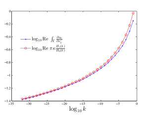
Fig. 1: $\displaystyle\log_{10}\mbox{Re }\int_{\Gamma}\frac{\partial u_{k}}{\partial x_{2}^{-}}$ (blue) against $\displaystyle\log_{10}\mbox{Re }\big{(}\pi k\frac{H_{1}(k)}{H_{0}(k)}\big{)}$ (red).

5 Asymptotics for high wavenumbers

We provide in this section a derivation of an equivalent for $\displaystyle\int_{\Gamma}\frac{\partial u_{k}}{\partial x_{2}^{-}}$ as $k\rightarrow\infty$, where $u_{k}=\tilde{u}_{k}+\varphi$, and $\tilde{u}_{k}$ solves variational problem (24). We will prove the following theorem

Theorem 5.1.

Let $\tilde{u}_{k}$ be the solution to (24), and set $u_{k}=\tilde{u}_{k}+\varphi$ .
The following estimates hold as $k$ approaches infinity,

$$\int_{\Gamma}\frac{\partial u_{k}}{\partial x_{2}^{-}}=-ik+O(k^{3/4}).$$ (45)

What is the asymptotic behavior of $\frac{\partial u_{k}}{\partial x_{2}^{-}}$ as the wavenumber $k$ approaches infinity? High frequency approximation for the wave equation is a vast subject which has been extensively studied over time. Historically, investigators have tried to explain how the laws of geometric optics relate to the wave equation at high frequency in an attempt to provide a sound foundation for Fresnel’s laws. Kirchhoff may have been the first one to write specific equations and asymptotic formulas for high frequency wave phenomena, however, his derivation was informal. A more mathematically rigorous study of the behavior of solutions to the wave equation at high frequency requires the use of Fourier integral operators and micro local analysis. As far as we know this kind of work was pioneered by Majda, Melrose and Taylor, see [10, 11, 12]. These authors were actually interested in the case of the exterior of a bounded convex domain, so their results can not be applied to our case since $\Gamma$ has empty interior in $\mathbb{R}^{2}$. We have instead to rely on recent groundbreaking work by Hewett, Langdony, and, Chandler-Wildez, see [5, 6] which pertains to either scattering in dimension 2 by soft or hard line segments (our case), or scattering in dimension 3 by soft or hard open planar surfaces. The great achievement of their work is that they were able to derive continuity and coercivity bounds that explicitly depend on the wavenumber.
Following the work by Hewett and Chandler-Wildez we introduce relevant functional spaces and frequency depending norms. Let $v$ be a tempered distribution on $\mathbb{R}$ and $\hat{v}$ its Fourier transform. Let $s$ be in $\mathbb{R}$. We say that $v$ is in $H^{s}(\mathbb{R})$ if $\int_{\mathbb{R}}(1+\xi^{2})^{s}|\hat{v}(\xi)|^{2}d\xi<\infty$. We then define in $H^{s}(\mathbb{R})$ the $k$ dependent norm

$$\|v\|_{H^{s}_{k}(\mathbb{R})}=(\int_{\mathbb{R}}(k^{2}+\xi^{2})^{s}|\hat{v}(\xi)|^{2}d\xi)^{1/2}.$$ (46)

Note that $H^{1}(\mathbb{R})$ is included in $H^{1/2}(\mathbb{R})$ and more precisely,

$$\|v\|_{H^{1/2}_{k}(\mathbb{R})}\leq k^{-1/2}\|v\|_{H^{1}_{k}(\mathbb{R})},$$ (47)

for all $v$ in $H^{1}(\mathbb{R})$. Denote by $I$ the interval $\displaystyle(-\frac{1}{2},\frac{1}{2})$. $\tilde{H}^{s}(I)$ is defined to be the closure of $C^{\infty}_{c}(I)$ (which is the space of smooth functions, compactly supported in $I$) for the norm $\|\|_{H^{s}_{k}(\mathbb{R})}$. ${H}^{s}(I)$ is defined to be the space of restrictions to $I$ of elements in $H^{s}(\mathbb{R})$. We define on ${H}^{s}(I)$ the norm

$$\|v\|_{H^{s}_{k}(I)}=\inf\{\|V\|_{H^{s}_{k}(\mathbb{R})}:V\in H^{s}_{k}(\mathbb{R})\mbox{ and }V|_{I}=v\}$$

Theorem 5.2.

(Hewett and Chandler-Wildez) For any $s$ in $\mathbb{R}$, the operator $S_{k}$ defined by the following formula for smooth functions $v$ on $I$

$$(S_{k}v)(x_{1})=\int_{I}\frac{i}{4}H_{0}(k|x_{1}-y_{1}|)v(y_{1})dy_{1}$$

can be extended to a continuous linear operator from $\tilde{H}^{s}(I)$ to $H^{s+1}(I)$. Furthermore, $S_{k}$ is injective, $S_{k}^{-1}$ is continuous and satisfies the estimate

$$\|S_{k}^{-1}v\|_{\tilde{H}^{-1/2}_{k}(I)}\leq 2\sqrt{2}\|v\|_{{H}^{1/2}_{k}(I)},$$ (48)

for all $v$ in $H^{1/2}_{k}(I)$.

Let us emphasize one more time that although the continuity and coercivity properties of $S_{k}$ have been known for some time, Hewett and Chandler-Wildez’s great achievement was to derive the dependency of the coercivity and the continuity bounds on the wavenumber $k$ as in estimate (48): the dependency appears in the use of the special norms $\|.\|_{{H}^{s}_{k}(I)}$.

5.1 An informal derivation of estimate (45)

This informal derivation will be helpful since it will give us an idea of what the asymptotic behavior of $\int_{\Gamma}\frac{\partial u_{k}}{\partial x_{2}^{-}}$ should be. Denote by $f_{k}(y_{1})$ the value of $\displaystyle\frac{\partial u_{k}}{\partial x_{2}^{-}}(y_{1},0)$ for $y_{1}$ in $I$. According to (31), $f_{k}$ satisfies the integral equation $S_{k}f_{k}=\frac{1}{2}$ or

$$\int_{I}\frac{i}{4}H_{0}(k|x_{1}-y_{1}|)f_{k}(y_{1})dy_{1}=\frac{1}{2},\quad x_{1}\in I$$ (49)

We multiply equation (49) by $-2ik$ and we integrate in $x_{1}$ over $I$ to obtain

$$\int_{I}\int_{I}\frac{k}{2}H_{0}(k|x_{1}-y_{1}|)f_{k}(y_{1})dy_{1}dx_{1}=-ik$$ (50)

If it is possible to interchange the order of integration in the left hand side of (50) then

$$\int_{I}\int_{I}\frac{k}{2}H_{0}(k|x_{1}-y_{1}|)dx_{1}f_{k}(y_{1})dy_{1}=-ik$$ (51)

Now for every $x_{1}$ in $I$, setting $v=k(x_{1}-y_{1})$ and using lemma 8.5 from the appendix, we find that

$$\lim_{k\rightarrow\infty}\int_{I}\frac{k}{2}H_{0}(k|x_{1}-y_{1}|)dx_{1}=1,$$

so we are led to believe that $\int_{I}f_{k}(y_{1})dy_{1}\sim-ik$, which we set out to prove in the next section.

5.2 Rigorous derivation of estimate (45)

Lemma 5.3.

The following estimate holds as $k$ approaches infinity

$$\|S_{k}(-ik)-\frac{1}{2}\|_{{H}^{1/2}_{k}(I)}=O(k^{1/4})$$ (52)

Proof: We start by recalling lemma 8.5 from the appendix and noting that for $x_{1}$ in I,

$$S_{k}(-ik)(x_{1})-\frac{1}{2}=\int_{I}\frac{1}{4}H_{0}(k|x_{1}-y_{1}|)kdy_{1}-\frac{1}{2}=-\int_{k(\frac{1}{2}+x_{1})}^{\infty}\frac{1}{4}H_{0}(v)dv-\int_{k(\frac{1}{2}-x_{1})}^{\infty}\frac{1}{4}H_{0}(v)dv$$

We now set $g_{k}(x_{1})=\int_{k(\frac{1}{2}+x_{1})}^{\infty}H_{0}(v)dv+\int_{k(\frac{1}{2}-x_{1})}^{\infty}H_{0}(v)dv$. Since the function $t\rightarrow\int_{t}^{\infty}H_{0}(v)dv$ is continuous on $[0,\infty)$ and has limit zero at infinity, there is a positive $C$ such that

$$|\int_{t}^{\infty}H_{0}(v)dv|\leq C,$$ (53)

for all $t$ in $[0,\infty)$. It is well known that as $v$ approaches infinity (see [1]), $H_{0}(v)=e^{i(v-\frac{\pi}{4})}\sqrt{\frac{2}{\pi v}}+O(v^{-\frac{3}{2}})$, so we also have the estimate

$$|\int_{t}^{\infty}H_{0}(v)dv|=O(t^{-\frac{1}{2}}),\quad t\rightarrow\infty$$ (54)

Without loss of generality we may assume that $k>4$. If $x_{1}$ is in $(-\frac{1}{2}+k^{-1/2},\frac{1}{2}-k^{1/2})$, then $k(\frac{1}{2}+x_{1})$ and $k(\frac{1}{2}-x_{1})$ are greater than $k^{1/2}$ so due to (54), $g_{k}(x_{1})=O(k^{-1/4})$. Then using (53) we infer that

$$\int_{I}|g_{k}|^{2}=\int_{(-\frac{1}{2}+k^{-1/2},\frac{1}{2}-k^{1/2})}|g_{k}|^{2}+\int_{I\setminus(-\frac{1}{2}+k^{-1/2},\frac{1}{2}-k^{1/2})}|g_{k}|^{2}=O(k^{-1/2})$$ (55)

Next we note that $g_{k}^{\prime}(x_{1})=kH_{0}(k(\frac{1}{2}+x_{1}))-kH_{0}(k(\frac{1}{2}-x_{1}))$. Using a substitution we find that

$$\int_{I}|g_{k}^{\prime}|^{2}\leq 4k\int_{0}^{k}|H_{0}(v)|^{2}dv$$

Given the asymptotics at infinity of $H_{0}$ we infer that

$$\int_{I}|g_{k}^{\prime}|^{2}=O(k\ln k),\quad k\rightarrow\infty$$ (56)

We now use (55) and (56) to evaluate a few Sobolev norms of $g_{k}$. We observe that $g_{k}(-\frac{1}{2})=g_{k}(\frac{1}{2})=\int_{0}^{\infty}H_{0}(v)dv+\int_{k}^{\infty}H_{0}(v)dv$ is uniformly bounded in $k$. We set for $k>0$

$$\tilde{g}_{k}(x_{1})=\left\{\begin{array}[]{ll}0&\mbox{ if }|x_{1}|\geq\frac{1}{2}+k^{-1/2}\\ k^{1/2}(x+\frac{1}{2}+k^{-1/2})g_{k}(\frac{1}{2})&\mbox{ if }-\frac{1}{2}-k^{-1/2}<x_{1}\leq-\frac{1}{2}\\ g_{k}(x_{1})&\mbox{ if }-\frac{1}{2}<x_{1}\leq\frac{1}{2}\\ -k^{1/2}(x-\frac{1}{2}-k^{-1/2})g_{k}(\frac{1}{2})&\mbox{ if }\frac{1}{2}<x_{1}<\frac{1}{2}+k^{-1/2}\end{array}\right.$$

Clearly, $\tilde{g}_{k}$ is in $H^{1}(\mathbb{R})$. A straightforward calculation will show that

$$\int_{\mathbb{R}\setminus I}|\tilde{g}_{k}|^{2}=O(k^{-1/2})\mbox{ and }\int_{\mathbb{R}\setminus I}|\tilde{g}_{k}^{\prime}|^{2}=O(k^{1/2})$$ (57)

Estimates (57) combined to (55) and (56) implies the following estimates for the Fourier transform of $\tilde{g}_{k}$

$$\int_{\mathbb{R}}|\widehat{\tilde{g}_{k}}(\xi)|^{2}d\xi=O(k^{-1/2})\mbox{ and }\int_{\mathbb{R}}\xi^{2}|\widehat{\tilde{g}_{k}}(\xi)|^{2}d\xi=O(k\ln k),$$ (58)

so

$$\int_{\mathbb{R}}(k^{2}+\xi^{2})|\widehat{\tilde{g}_{k}}(\xi)|^{2}d\xi=O(k^{3/2}),$$

that is, $\|\tilde{g}_{k}\|_{{H}^{1}_{k}(\mathbb{R})}=O(k^{3/4})$. Now, due to inequality (47), $\|\tilde{g}_{k}\|_{{H}^{1/2}_{k}(\mathbb{R})}=O(k^{1/4})$ and estimate (52) is proved. $\square$

Lemma 5.4.

The following estimate holds as $k$ approaches infinity

$$\|1\|_{{H}^{1/2}_{k}(I)}=O(k^{1/2})$$ (59)

Proof: We set for $k>0$

$$h(x_{1})=\left\{\begin{array}[]{ll}0&\mbox{ if }|x_{1}|\geq 1\\ 2(x+1)&\mbox{ if }-1<x_{1}\leq-\frac{1}{2}\\ 1&\mbox{ if }-\frac{1}{2}<x_{1}\leq\frac{1}{2}\\ -2(x-1)&\mbox{ if }\frac{1}{2}<x_{1}<1\end{array}\right.$$

Clearly $h$ is in $H^{1}(\mathbb{R})$ and is independent of $k$ so

$$\int_{\mathbb{R}}|\widehat{h}(\xi)|^{2}d\xi=O(1)\mbox{ and }\int_{\mathbb{R}}\xi^{2}|\widehat{h}(\xi)|^{2}d\xi=O(1)$$ (60)

From there we infer $\|h\|_{H^{1/2}_{k}(\mathbb{R})}=O(k^{1/2})$ and estimate (59) is proved. $\square$

Proof of theorem 5.1:
Combining estimates (48) and (52) and recalling that $S_{k}f_{k}=\frac{1}{2}$ we may write

$$\|-ik-f_{k}\|_{\tilde{H}^{-1/2}_{k}(I)}=O(k^{1/4})$$ (61)

We then use estimate (59) and we write denoting by $<,>$ the duality bracket $\tilde{H}^{-1/2}_{k}(I),H^{1/2}_{k}(I)$

$$<-ik-f_{k},1>=O(k^{3/4})$$ (62)

Following [7], there are two constants $C_{1}$ and $C_{2}$ such that

$$f_{k}-C_{1}(\frac{1}{2}-x_{1})^{-1}-C_{2}(\frac{1}{2}+x_{1})^{-1}$$

is in $H^{1/2}_{k}(I)$. In particular $f_{k}$ is in $L^{q}(I)$ for every $q$ in $[1,2)$, so $\int_{I}f_{k}$ is a regular Lebesgue integral. Since $I$ has measure 1, estimate (45) follows from (62). $\square$

For illustration, figure 2 shows a graph of the imaginary part and a graph of the real part of $\displaystyle\frac{1}{k}\int_{-\frac{1}{2}}^{\frac{1}{2}}f_{k}(y_{1})dy_{1}$, that is, $\displaystyle\frac{1}{k}\int_{\Gamma}\frac{\partial u_{k}}{\partial x_{2}^{-}}$, against the wavenumber $k$. See [14] and [4] for the numerical method that we used.

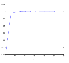
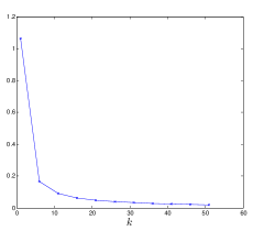
Fig. 2: Left: computed values of $\displaystyle\frac{1}{k}Im\int_{\Gamma}\frac{\partial u_{k}}{\partial x_{2}^{-}}$ against $k$. Right: computed values of $\displaystyle\frac{1}{k}Re\int_{\Gamma}\frac{\partial u_{k}}{\partial x_{2}^{-}}$ against $k$.

6 Proof of theorem 2.1

6.1 The case $C_{1},C_{2},C_{3},C_{4}>0$

In this section we cover the case where the constants $C_{1},C_{2},C_{3},C_{4}$ are all positive, which was assumed in theorem 2.1. We explained in section 4 how the function $\Phi$ defined by (1-4) relates to $u_{k}$ where $u_{k}=\tilde{u}_{k}+\varphi$ and $\tilde{u}_{k}$ solves (24): if $u_{k}$ is extended to $\mathbb{R}^{2}$ as indicated by lemma 4.3 then $u_{k}$ and $\Phi$ are equal on $\overline{\mathbb{R}^{2+}}$. Accordingly, recalling the definition of the function $F$ given in (7) and formula (30), $F$ can also be expressed as follows,

$$F(k)=q(k^{2})+p(k^{2})\mbox{Re }\int_{\Gamma}\frac{\partial u_{k}}{\partial x_{2}^{-}}$$ (63)

We know from lemma 4.4 that $F$ is analytic in $(0,\infty)$. Recalling the definition of $p$ and $q$, (6), and using estimate (44) we have that

$$F(k)\sim C_{2}\pi(\ln k)^{-1},\quad k\rightarrow 0^{+}$$ (64)

Recalling estimate (45) we claim that

$$F(k)\sim C_{3}k^{4},\quad k\rightarrow\infty$$ (65)

It follows from estimate (64) that there is a positive $\alpha$ such that $F(k)<0$ if $k$ is in $(0,\alpha)$, and from estimate (65) we infer that $\lim_{k\rightarrow\infty}F(k)=\infty$. Since $F$ is continuous in $(0,\infty)$, we conclude that $F$ must achieve the value zero on that interval. We can also claim that the zeros of $F$ are isolated since $F$ is an analytic function. Due to (65) these zeros occur only in some interval $[A,B]$ where $A$ and $B$ are two positive constants. In particular the equation $F(k)=0$ has at most a finite number of solutions.
For illustration, figure 3 shows $\log_{10}|F(k)|$ and $\log_{10}(C_{2}\pi|\ln k|^{-1})$ against $\log_{10}k$ on the left, and $\log_{10}\big{|}F(k)\big{|}$ and $\log_{10}(C_{3}k^{4})$ against $k$ on the right. These graphs were produced using the specific constants $C_{1}=0.4,C_{2}=2/3,C_{3}=5/12,C_{4}=5/48$, see [16] and [14] for why this choice is physically plausible.

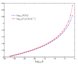
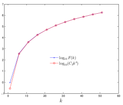
Fig. 3: Numerical computations illustrating formulas (64) and (65). These graphs were produced using the specific constants $C_{1}=0.4,C_{2}=2/3,C_{3}=5/12,C_{4}=5/48$, see [16] and [14] for why this choice is physically plausible and for a description of the numerical method employed. Left: $\log_{10}|F(k)|$ (blue) vs $\log_{10}(C_{2}\pi|\ln k|^{-1})$ (red). Right: $\log_{10}F(k)$ (blue) vs $\log_{10}(C_{3}k^{4})$ (red).

6.2 Use of estimates in the case where $C_{3}<0$

We first claim that for any positive value of $C_{1},C_{2},C_{4}$, there exist negative values of $C_{3}$, such that the equation $F(k)=0$ has no solutions. According to estimate (44) there is a positive $\alpha$ such that for all $k$ in $(0,\alpha)$,

$$-\frac{1}{2}\pi(\ln k)^{-1}\leq\mbox{Re }\int_{\Gamma}\frac{\partial u_{k}}{\partial x_{2}^{-}}\leq-\frac{3}{2}\pi(\ln k)^{-1}.$$ (66)

Consequently for $k$ in $(0,\alpha)$,

$$F(k)\leq C_{4}k^{2}+C_{1}k^{2}(-\frac{3}{2}\pi(\ln k)^{-1})+C_{2}\frac{1}{2}\pi(\ln k)^{-1}$$ (67)

so if $\alpha$ is small enough, $F(k)<0$ if $k$ is in $(0,\alpha)$. According to (45) there is a negative $A_{1}$ and a positive $A_{2}$ such that for all k in $[\alpha,\infty)$,

$$A_{1}k^{3/4}\leq\mbox{Re }\int_{\Gamma}\frac{\partial u_{k}}{\partial x_{2}^{-}}\leq A_{2}k^{3/4}.$$ (68)

so for all k in $[\alpha,\infty)$,

$$F(k)\leq C_{3}k^{4}+C_{4}k^{2}+C_{1}A_{2}k^{2+3/4}-C_{2}A_{1}k^{3/4}$$ (69)

so if we choose $C_{3}$ less than some negative constant, $F(k)<0$ for all k in $[\alpha,\infty)$. We conclude that for that choice of $C_{3}$, $F(k)<0$ for all positive $k$, so the equation $F(k)=0$ has no solution in $(0,\infty]$.

Next we show the following claim: for any value of the positive constants $C_{1},C_{2}$ and any value of the negative constant $C_{3}$, for all values of $C_{4}$ greater than some constant, the equation $F(k)=0$ has at least one solution. We may assume that $\alpha$ defined above is less than 1. For all k in $[\alpha,\infty)$

$$F(k)\geq C_{3}k^{4}+C_{4}k^{2}+C_{1}A_{1}k^{2+3/4}-C_{2}A_{2}k^{3/4}$$ (70)

thus $F(1)>0$ for any $C_{4}$ greater than some constant. As $C_{3}<0$, thanks to (69), we have that, $\lim_{k\rightarrow\infty}F(k)=-\infty$, so by continuity of $F$ we conclude that the equation $F(k)=0$ has at least one solution in $(0,\infty)$.

7 Conclusion and perspectives

We have proved in this paper the existence of frequency modes coupling seismic waves and vibrating tall buildings. Although the derivation from physical principles of a set of equations modeling this phenomenon was carefully done and numerical evidence supporting existence of coupling frequency modes was shown in previous studies, to the best of our knowledge, up to now, there was no formal proof of existence.
We believe that only minor modifications to our present argument would show existence of coupling frequency modes in the case of a finite set of buildings. The present study was limited to a single building chiefly for clarity of exposition. It could turn out, however, that the case of a periodically repeated pattern of buildings might involve more substantial alterations of the existence proof given in this paper. Note that this case was particularly important in our simulations of coupling modes presented in [14].
Recalling that our study pertains exclusively to anti plane shearing, it will be important to generalize our results to fully three dimensional elastic vibrations. At present, this appears to be quite an undertaking given the complexity of Green’s tensor for half space elasticity and the lack of a known analog to theorem 5.2 for the elasticity operator.

8 Appendix: useful results on Hankel functions

For $n\in\mathbb{N}$ and $z$ in $\mathbb{C}$ we denote by $J_{n}$ the Bessel function

$$J_{n}(z)=(\frac{1}{2}z)^{n}\sum_{k=0}^{\infty}(-\frac{1}{4})^{k}\frac{z^{2k}}{k!(n+k)!}$$

For $n\in\mathbb{N}$ and $z$ in $\mathbb{C}\setminus\mathbb{R}^{-*}$ we denote by $Y_{n}$ the Bessel function

$$-\frac{1}{\pi}(\frac{1}{2}z)^{-n}\sum_{k=0}^{n-1}\frac{(n-k-1)!}{k!}(\frac{1}{4}z^{2})^{k}+\frac{2}{\pi}\ln(\frac{1}{2}z)J_{n}(z)$$

$$-\frac{1}{\pi}(\frac{1}{2}z)^{n}\sum_{k=0}^{\infty}(\psi(k+1)+\psi(n+k+1))(-\frac{1}{4})^{k}\frac{z^{2k}}{k!(n+k)!},$$

where the first sum is void if $n=0$ and the function $\psi$ is defined by

$$\psi(1)=-\gamma,\,\psi(n)=-\gamma+\sum_{k=1}^{n-1}\frac{1}{k},$$

and $\gamma$ is the Euler constant. The Hankel function of the first kind of order $n$, that is, $J_{n}+iY_{n}$, will be denoted $H_{n}$.

Lemma 8.1.

The following equivalence as $n\rightarrow\infty$ is uniform for all $z$ in a compact set of $(0,\infty)$

$$H_{n}(z)\sim-\frac{i}{\pi}(\frac{1}{2}z)^{-n}(n-1)!$$ (71)

Proof: Since for any positive $z$

$$|J_{n}(z)n!(\frac{1}{2}z)^{-n}-1|=\frac{1}{n+1}|\sum_{k=1}^{\infty}(-\frac{1}{4})^{k}\frac{z^{2k}(n+1)!}{k!(n+k)!}|$$

$$\leq\frac{1}{n+1}\sum_{k=1}^{\infty}(\frac{1}{4})^{k}\frac{z^{2k}}{k!}$$

it is clear that $\displaystyle J_{n}(z)\sim(\frac{1}{2}z)^{n}\frac{1}{n!}$ uniformly for all $z$ in a compact set of $(0,\infty)$.
We can show similarly that $\displaystyle Y_{n}(z)\sim-\frac{1}{\pi}(\frac{1}{2}z)^{-n}(n-1)!$ uniformly for all $z$ in a compact set of $(0,\infty)$. We conclude that (71) must hold. $\square$

Lemma 8.2.

For $z>0$, the following limit as $z\rightarrow 0$ is uniform for all integers $n$ different from 0

$$\lim_{z\rightarrow 0^{+}}-\frac{z}{|n|}\frac{H_{n}^{\prime}(z)}{H_{n}(z)}=1$$ (72)

For the special case $n=0$ we have,

$$\lim_{z\rightarrow 0^{+}}\frac{zH_{0}^{\prime}(z)}{H_{0}(z)}=0$$

Proof: We observe that for $n\geq 2$

$$\left(H_{n}(z)(-\frac{i}{\pi}(\frac{1}{2}z)^{-n}(n-1)!)^{-1}-1\right)(n-1)$$

can be bounded by a function in $z$ which is continuous on $[0,\infty)$ and independent of $n$, therefore

$$H_{n}(z)\sim-\frac{i}{\pi}(\frac{1}{2}z)^{-n}(n-1)!$$ (73)

as $z\rightarrow 0^{+}$, uniformly on $[0,b]$ for a fixed $b>0$. Using the formula

$$H_{n}^{\prime}(z)=-H_{n+1}(z)+\frac{n}{z}H_{n}(z)$$ (74)

we obtain

$$-\frac{z}{n}\frac{H_{n}^{\prime}(z)}{H_{n}(z)}\sim 1$$

as $z\rightarrow 0^{+}$, uniformly on $[0,b]$ for a fixed $b>0$.
For $n\leq-2$, we can now apply the formula $H_{-n}(z)=(-1)^{n}H_{n}(z)$. The remaining three cases can be treated in a straightforward fashion. $\square$

Lemma 8.3.

For any $n$ in $\mathbb{N}$, $|H_{n}(z)|$ is a decreasing function of $z$ on $(0,+\infty)$.

Proof: This is due to the formula derived by Nicholson, see [15],

$$J_{n}^{2}(z)+Y_{n}^{2}(z)=\frac{8}{\pi^{2}}\int_{0}^{\infty}K_{0}(2z\sinh t)\cosh 2ntdt$$

where $\displaystyle K_{0}(s)=\int_{0}^{\infty}e^{-s\cosh t}dt$. $\square$

Lemma 8.4.

Let $a$ and $b$ be two real numbers such that $0<a<b$. The following equivalence as $n\rightarrow\infty$ is uniform for all complex numbers $z$ in the closed disk of the complex plane centered at $b$ and of radius $a$

$$H_{n}(z)\sim-\frac{i}{\pi}(\frac{1}{2}z)^{-n}(n-1)!$$ (75)

Proof: The proof is nearly identical to that of lemma 8.1. $\square$

Lemma 8.5.

Denote by $\mbox{St}_{n}$ the Struve function of order $n$ as defined in [1]. The following formula holds for any $t>0$

$$\int_{0}^{t}H_{0}(z)dz=tH_{0}(t)+\frac{\pi}{2}t(\mbox{St}_{0}H_{1}(t)-\mbox{St}_{1}H_{0}(t))$$ (76)

It follows that the semi convergent integral $\displaystyle\int_{0}^{\infty}H_{0}(z)dz$ is exactly equal to $1$.

Proof: Integral formula (76) is given in [1]. The value of $\int_{0}^{\infty}H_{0}(z)dz$ results from that formula combined to known asymptotics at infinity of Bessel and of Struve functions. One should consult [1] for formulas on Bessel functions, and [15] for their derivation. $\square$

References

- [1] M. Abramowitz and I. Stegun, eds. (1992), Handbook of Mathematical Functions with Formulas, Graphs, and Mathematical Tables, Dover, New York.
- [2] S. Erlingsson, A. Bodare, Live load induced vibrations in Ullevi Stadium - dynamic underground analysis, underground Dyn. and Earthquake Eng., vol. 15, Issue 3 (1996) 171-188.
- [3] G. B. Folland, Introduction to Partial Differential Equations, Second Edition, Princeton University Press.
- [4] M. Ghergu, I. R. Ionescu, Structure-underground-structure coupling in seismic excitation and ”city-effect”. Int. J. Eng. Sci. 47 (2009) 342-354.
- [5] D. P. Hewett, S. N. Chandler-Wilde, Acoustic scattering by fractal screens: mathematical formulations and wavenumber-explicit continuity and coercivity estimates, arXiv.org ¿ math ¿ arXiv:1401.2805, 2014.
- [6] D. P. Hewett, S. Langdon, S. N. Chandler-Wilde, A frequency-independent boundary element method for scattering by two-dimensional screens and apertures, arXiv.org ¿ math ¿ arXiv:1401.2786, 2014.
- [7] G. Hsiao, E. P. Stephan, W. L. Wendland, On the Dirichlet problem in elasticity for a domain exterior to an arc, Journal of Computational and Applied Mathematics, Volume 34, Issue 1, 10 February 1991, pp. 1-19
- [8] H. Kanamori, J. Mori, B. Sturtevant, D. L. Anderson, T. Heaton, Seismic excitation by space shuttles, Shock waves, 2 (1992) 89-96.
- [9] T. Kato, Perturbation theory for linear operators, Grundlehren Math. Wiss., Vol. 132. Springer, 1995.
- [10] A. Majda, High frequency asymptotics for the scattering matrix and the inverse problem of acoustical scattering, Communications on Pure and Applied Mathematics, Volume 29, Issue 3, 261-291, 1976.
- [11] A. Majda, M. E. Taylor, The asymptotic behavior of the diffraction peak in classical scattering, Communications on Pure and Applied Mathematics, Volume 30, Issue 5, 639-669, 1977
- [12] Richard B Melrose, Michael E Taylor, Near peak scattering and the corrected Kirchhoff approximation for a convex obstacle, Advances in Mathematics Volume 55-3, 1985, 242-315.
- [13] Giovanni Maria Troianiello, Elliptic Differential Equations and Obstacle Problems, University Series in Mathematics, 1987.
- [14] D. Volkov and S. Zheltukhin, Preferred Frequencies for Coupling of Seismic Waves and Vibrating Tall Buildings, submitted. (submission available on arXiv.org)
- [15] G. N. Watson, A treatise on the theory of Bessel functions, Cambridge University press, 1922.
- [16] S. Zheltukhin, Preferred Frequencies for Coupling of Seismic Waves and Vibrating Tall Buildings, PhD. thesis, WPI, 2013.