Dynamical Mean Field Theory for Diatomic Molecules and the Exact Double Counting

Abstract

Dynamical mean field theory (DMFT) combined with the local density approximation (LDA) is widely used in solids to predict properties of correlated systems. In this study, a parameter-free version of LDA+DMFT framework is implemented and tested on one of the simplest strongly correlated systems, H₂ molecule. Specifically, we propose a method to calculate the exact intersection of LDA and DMFT that leads to highly accurate subtraction of the doubly counted correlation in both methods. When the exact double-counting treatment and a good projector to the correlated subspace are used, LDA+DMFT yields very accurate total energy and excitation spectrum of H₂. We also discuss how this double-counting scheme can be extended to solid state calculations.

I Introduction

Quantum mechanics has long sought deeper insight into correlation effects because they lie at the heart of understanding atomic, molecular and solid state electronic structure. Over the past few decades, many theoretical frameworks have been developed to describe so-called “strongly correlated systems”, in which quasi-particle approaches such as density functional theory (DFT) Hohenberg and Kohn (1964); Kohn and Sham (1965) essentially fail due to the large Coulomb interaction between electrons. Among them, dynamical mean field theory (DMFT) Georges and Kotliar (1992); Georges et al. (1996) has brought about a revolution in the theory of strong correlations after its exact treatment of local dynamic correlations successfully described the Mott transition in lattice models such as the Hubbard model Kotliar and Vollhardt (2004). Since the method is very flexible and versatile, and scales linearly with the system size, it has been quickly adapted for many solid state problem, including electronic structure calculations.

The most commonly used DMFT approximation in solid state is combination of LDA and DMFT (LDA+DMFT) Kotliar et al. (2006), where some selected correlated orbitals are treated by DMFT while the rest of the electronic states are treated by LDA. The LDA+DMFT method has been very successful in various problems involving strong electronic correlations in solids and very recently it was also applied to molecules Lin et al. (2011); Zgid and Chan (2011) and nano-systems Jacob et al. (2010); Turkowski et al. (2012). However, the application of this methodology to solids has a few ambiguities, which limit the precision of the method: i) the DMFT method needs the partially screened Coulomb interaction, which is hard to predict from first principles, ii) the part of the correlations treated by both LDA and DMFT – called double-counting – is not known exactly, and a phenomenological form Anisimov et al. (1997) has been most often used (for discussion see Haule et al. (2014) and Dang et al. (2014)).

The study of correlations in small molecules can be a testbed for the quality of electronic structure methods because numerically exact results exist. From the DMFT view point, this has a particularly strong appeal because the screening of the Coulomb repulsion can be negligible and therefore the ambiguities due to screening, present in solid state, can be decoupled from the issues concerning construction of the functional and its precision. In addition, the short-range nature of dynamical correlation in molecules Stollhoff and Fulde (1977, 1978) further justifies the applicability of DMFT to molecules. While H_n clusters Lin et al. (2011) and H- cubic solid Zgid and Chan (2011) have been investigated within the DMFT framework, the simplest case of H₂ molecule, which shows very strong correlations at large nuclear separation, has not been studied yet by DMFT.

In this paper we propose a double-counting functional for LDA+DMFT, which is an exact intersection of the two methods and results in highly precise electronic structure method with no ambiguity in subtracting doubly counted correlation effect. We also suggest the extension of this double-counting functional to the solid state calculations, where additional complexity of screening will need to be addressed. Our basis set is the eigenfunctions of H${}_{2}^{+}$ exactly solved by the methodology of Ref. Hadinger et al., 1989. We denote the ground state and the first excited state by $\ket{1\sigma_{g}}$ and $\ket{1\sigma_{u}}$, respectively. Typically between other 20-30 excited states are used as a basis for H₂ calculation for good convergence.

Since DMFT is a basis set dependent approximation, its quality depends essentially on the choice of the projector Paul and Kotliar (2006); Haule et al. (2010); Marzari and Vanderbilt (1997); Pavarini et al. (2004); Anisimov et al. (2005); Amadon et al. (2008), which maps the continuous problem to a discrete set of sites (lattice), each consisting of only a few important degrees of freedom (orbitals). In this work, we restrict our discussion to the simplest possible DMFT approximation, taking only one correlated orbital per site. Since the two sites are equivalent by the symmetry, the problem reduces to a single site one orbital impurity problem, which can be solved to very high precision by the continuous time quantum Monte Carlo method Werner and Millis (2006), as implemented in Ref. Haule, 2007.

II Theory and Method

A good choice of the DMFT projector should have large overlap with the most active states around the Fermi level, should be well localized on an atom, recover atomic solution in the large separation limit, and finally should not depend on the self-consistent charge density. Without the last condition, it is impossible to obtain a stationary solution by extremizing Luttinger-Ward functional.

A natural choice of the DMFT projector of this H₂ problem is the linear combination of the lowest bonding $\ket{1\sigma_{g}}$ and anti-bonding state $\ket{1\sigma_{u}}$ of H${}_{2}^{+}$ system, which we define as the “left” (L) and the “right” (R) localized orbital,

$$|\chi_{L}\rangle=\frac{1}{\sqrt{2}}(|1\sigma_{g}\rangle-|1\sigma_{u}\rangle),$$

$$|\chi_{R}\rangle=\frac{1}{\sqrt{2}}(|1\sigma_{g}\rangle+|1\sigma_{u}\rangle).$$ (1)

that naturally recover 1$s$ state of each site at large atomic separation. Over 96% of the electronic charge of the DMFT solution is contained in these two states and since they do not explicitly depend on the DMFT Green’s function, these are a good choice for DMFT orbital.

We define the DMFT local Green’s function for left atom by the projection ${\cal G}^{L}_{local}(\omega)\equiv\hat{P}_{L}G=\ket{\chi_{L}}\bra{\chi_{L}}G(\textbf{r},\textbf{r}^{\prime},\omega)\ket{\chi_{L}}\bra{\chi_{L}}$ and similarly for the right atom. The impurity self-energy is embedded into real space by the inverse of the projection, i.e., $\Sigma(\textbf{r},\textbf{r}^{\prime},\omega)=\ket{\chi_{L}}\Sigma^{L}(\omega)\bra{\chi_{L}}+\ket{\chi_{R}}\Sigma^{R}(\omega)\bra{\chi_{R}}$. Due to the symmetry of the problem, $\Sigma^{L}=\Sigma^{R}$ and $G^{L}=G^{R}$. We mention in passing that the alternative choice of projector, which selects as the correlated orbital $1s$ state of each atom, leads to a result of worse quality than presented here, because such choice does not capture the majority of the active degrees of freedom at equilibrium internuclear separation. Consequently, more time consuming cluster-DMFT method needs to be used to obtain similar quality results, as recently found in Ref. Lin et al., 2011.

To construct the DMFT framework, we resort to the Baym-Kadanoff formalism Baym and Kadanoff (1961); Baym (1962), which defines a functional of the full Green’s function by (see also Kotliar et al. (2006))

$$\Gamma[G]={\mathrm{Tr}}\log(G)-{\mathrm{Tr}}((G^{-1}_{0}-G^{-1})G)+\Phi[G].$$ (2)

Here $G_{0}(\mathbf{r},\mathbf{r}^{\prime};i\omega)=[(i\omega+\mu+\nabla^{2}-V_{ext}(\mathbf{r}))\delta(\mathbf{r}-\mathbf{r}^{\prime})]^{-1}$, and $V_{ext}$ is the potential created by the two nucleus. $\Phi[G]$ is the so-called Luttinger-Ward functional and is equal to the sum of all skeleton Feynman diagrams consisting of $G$ and Coulomb interaction $U_{C}$. $\Gamma[G]$ is extremized by the exact Green’s function and gives the free energy of the system in the extremum.

First, we discuss the Hartree-Fock approximation. In this case, $\Phi[G]=\Phi^{H}[\rho]+\Phi^{X}[\rho]$, where $\Phi^{H}[\rho]=\frac{1}{2}\int_{\textbf{r}\textbf{r}^{\prime}}\rho(\mathbf{r})U_{C}(\textbf{r}-\textbf{r}^{\prime})\rho(\mathbf{r}^{\prime})$ and $\Phi^{X}[\rho]=-\frac{1}{2}\sum_{\sigma}\int_{\textbf{r}\textbf{r}^{\prime}}\rho^{\sigma}(\textbf{r},\textbf{r}^{\prime})U_{C}(\textbf{r}-\textbf{r}^{\prime})\rho^{\sigma}(\textbf{r}^{\prime},\textbf{r})$. Here $U_{C}=\frac{2}{|\textbf{r}-\textbf{r}^{\prime}|}$ is the Coulomb repulsion, $\rho(\mathbf{r},\mathbf{r}^{\prime})=T\sum_{n}G(\mathbf{r},\mathbf{r}^{\prime};i\omega_{n})e^{i\omega_{n}0^{+}}$ is the single particle density matrix and $\rho(\textbf{r})=\rho(\textbf{r},\textbf{r})$ is the electronic density.

Next we discuss the LDA approximation, in which $\Phi[G]$ is approximated by the sum of the Hartree $\Phi^{H}[\rho]$, local exchange $\Phi^{LDA,X}[\rho]=\int_{\textbf{r}}\rho(\textbf{r})\varepsilon_{x}(\rho(\textbf{r}))$ and local correlation $\Phi^{LDA,C}[\rho]=\int_{\textbf{r}}\rho(\textbf{r})\varepsilon_{c}(\rho(\textbf{r}))$ functional. Here, we use the Slater exchange functional, $\varepsilon_{x}(\rho)=-\frac{3}{2}(\frac{3}{\pi}\rho)^{\frac{1}{3}}$, and the Vosko-Wilk-Nusair (VWN) parametrization Vosko et al. (1980) for the correlation functional $\varepsilon_{c}(\rho)$.

DMFT approximates the exact Luttinger functional $\Phi[G]$ by its local counterpart $\Phi^{DMFT}=\sum_{i}\Phi[{\cal G}^{i}_{local}]$ Kotliar et al. (2006), which contains all skeleton Feynman diagrams constructed from the local Green’s function ${\cal G}^{i}_{local}$ centered on the local site $i$, and the local Coulomb repulsion $U^{i}_{local}=\bra{\chi_{i}\chi_{i}}U_{C}(\textbf{r}-\textbf{r}^{\prime})\ket{\chi_{i}\chi_{i}}$. Notice that the exact functional $\Phi$ and the DMFT functional $\Phi^{DMFT}$ have exactly the same topological structure in terms of Feynman diagrams. The only difference is that $\Phi$ is a functional of full Green’s function $G$ and $U_{C}$ while $\Phi^{DMFT}$ is a functional of ${\cal G}^{i}_{local}$ and $U^{i}_{local}$. The essential DMFT variable is ${\cal G}^{i}_{local}$, which is computed by the projection discussed above, and is being matched with the auxiliary impurity Green’s function.

The flexibility of the DMFT approximation allows one to treat some parts of the functional exactly, such as the Hartree-Fock terms. This approximation is denoted by HF+DMFT, i.e., $\Phi^{HF+DMFT}[G]=\Phi^{H}[\rho]+\Phi^{X}[\rho]+\sum_{i}\Phi^{DMFT}[{\cal G}_{local}^{i}]-\sum_{i}\Phi^{DC}[\rho^{i}_{local}]$. Since local part of the Hartree and exchange term is present also in DMFT, we have to subtract terms counted twice $\Phi^{DC}[\rho^{i}_{local}]=\Phi^{H}[\rho^{i}_{local}]+\Phi^{X}[\rho^{i}_{local}]$, where $\rho^{i}_{local}=\ket{\chi_{i}}\bra{\chi_{i}}\rho\ket{\chi_{i}}\bra{\chi_{i}}$, $\Phi^{H}[\rho^{i}_{local}]=\frac{1}{2}\int_{\textbf{r}\textbf{r}^{\prime}}\rho^{i}_{local}(\textbf{r})U_{C}(\textbf{r}-\textbf{r}^{\prime})\rho^{i}_{local}(\textbf{r}^{\prime})$ and $\Phi^{X}[\rho^{i}_{local}]=-\frac{1}{2}\sum_{\sigma}\int_{\textbf{r}\textbf{r}^{\prime}}\rho^{\sigma,i}_{local}(\textbf{r},\textbf{r}^{\prime})U_{C}(\textbf{r}-\textbf{r}^{\prime})\rho^{\sigma,i}_{local}(\textbf{r}^{\prime},\textbf{r})$.

Finally, we define the functional of the combination of LDA and DMFT, i.e., LDA+DMFT, in which the DMFT correlations (truncated to small subset of important degrees of freedom) and LDA static correlations complement each other. The functional is $\Phi^{LDA+DMFT}[G]=\Phi^{H}[\rho]+\Phi^{X}[\rho]+\Phi^{LDA,C}[\rho]+\sum_{i}\Phi^{DMFT}[{\cal G}^{i}_{local}]-\sum_{i}\Phi^{DC}[\rho^{i}_{local}]$ where the exact-exchange functional $\Phi^{X}[\rho]$ is used because the non-local exchange is large in molecular systems. The doubly counted correlation term is contained in $\Phi^{DC}[\rho^{i}_{local}]=\Phi^{H}[\rho^{i}_{local}]+\Phi^{X}[\rho^{i}_{local}]+\Phi^{LDA,C}[\rho^{i}_{local}]$, where $\Phi^{H}$ and $\Phi^{X}$ are defined above, and the double-counted correlation is

$$\Phi^{LDA,C}[\rho^{i}_{local}]=\int_{\textbf{r}}\varepsilon_{c}(\rho^{i}_{local}(\textbf{r}))\rho^{i}_{local}(\textbf{r}).$$ (3)

This is the exact intersection between LDA and DMFT approximation since it parallels the derivation of the DMFT approximation starting from the exact functional (For details, see Appendix). The double-counting term is hence a “DMFT”-like approximation to the LDA correlation functional. Namely, just as the replacement of the total $G$ by its local counterpart ${\cal G}^{i}_{local}$ in the exact functional leads to the DMFT approximation, replacing total $\rho$ by $\rho^{i}_{local}$ in LDA functional gives the intersection of the two methods.

Although LDA+DMFT is very often used in solid-state electronic structure calculations, such an exact double-counting term has not been proposed before. This is because in the solids, there is additional complexity of screening, whereby the core, semicore and other states excluded by the DMFT model screen the Coulomb interaction in the DMFT correlated space. Therefore the derivation of the DMFT Luttinger-Ward functional in solids requires not only the substitution of the total Green’s function $G$ by ${\cal G}_{local}$ but also unscreened Coulomb repulsion $U_{C}=\frac{2}{|\textbf{r}-\textbf{r}^{\prime}|}$ by screened one ${\cal U}_{C}=\frac{2e^{-\lambda|\textbf{r}-\textbf{r}^{\prime}|}}{|\textbf{r}-\textbf{r}^{\prime}|}$.

For solid state calculations, we propose to approximate the double-counting functional by a similar functional as in Eq. 3, but with $\varepsilon_{c}$ being a function of density and screening length $1/\lambda$, i.e., $\varepsilon_{c}(\rho_{local}(\textbf{r}),{\cal U}(\lambda))$. This requires calculation of the correlation density for the electron gas model by quantum Monte Carlo in two dimensional space, as a function of density $r_{s}$ and screening $\lambda$. The same screened form of the Coulomb repulsion has to be then used in the DMFT impurity calculation, i.e., ${\cal U}_{m_{1}m_{2}m_{3}m_{4}}=\bra{m_{1}m_{2}}\frac{2e^{-\lambda|\textbf{r}-\textbf{r}^{\prime}|}}{|\textbf{r}-\textbf{r}^{\prime}}\ket{m_{3}m_{4}}$. Notice that the screening length $\lambda$ is uniquely determined by the screened Coulomb parameter ${\cal U}$, which can be estimated by constrained LDA Gunnarsson et al. (1989) or constrained RPA Aryasetiawan et al. (2004).

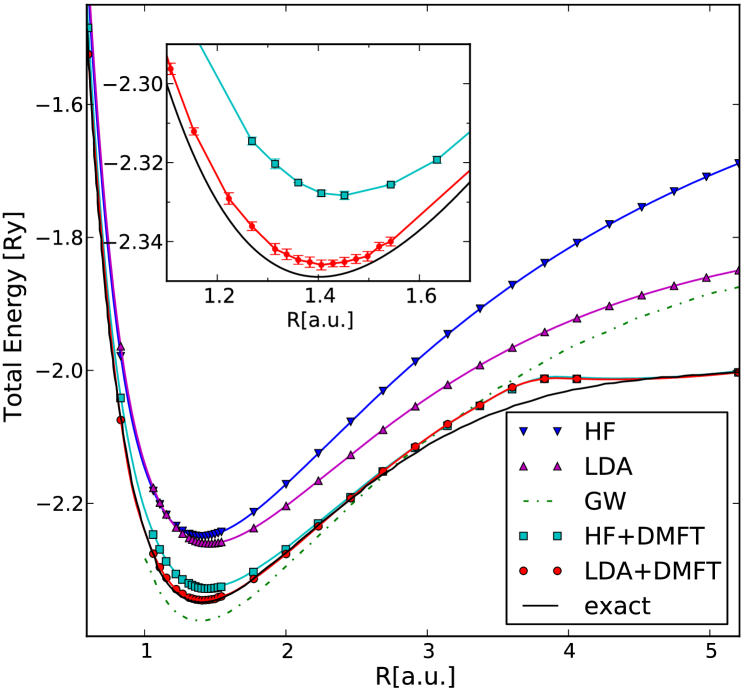
Figure 1: (Color online) Total energy curves of the H₂ molecule versus interatomic distance $R$ calculated by different methods: LDA+DMFT, HF+DMFT, LDA, and HF. The GW and exact result are also presented for comparison.

III Results

In Fig. 1 we compare the total energy curves of the H₂ molecule versus nuclear separation obtained by different electronic structure methods to the exact result from Ref. Kolos and Wolniewicz, 1964. The Hartree-Fock method describes the equilibrium distance quite well ($R\approx 1.39$ compared to exact $1.402$), but the energy is severely overestimated, in particularly upon dissociation. This well-known problem is attributed to static correlation that arises in situations with degeneracy or near-degeneracy, as in many transition metal solids and strongly correlated systems.

Due to missing correlations, at large distance the Hartree-Fock method predicts that the two electrons is both found at one nucleus with the same probability as finding them away from each at its own nucleus. By including static local correlations, the LDA method improves on the energy at large distance, although it is still way higher than the energy of two hydrogen atoms. The equilibrium distance is overestimated by LDA ($R\approx 1.46$) and the total energy at equilibrium is similar to its Hartree-Fock value. We also include in the plot the result of the self-consistent GW calculation from Ref. Stan et al., 2009, which gives a quite lower total energy at equilibrium and severely overestimated dissociation energy which is comparable to that of LDA.

At large interatomic separation, the static correlations are not adequate because of the near-degeneracy of many body states, which can not be well described by electron density alone. The DMFT uses the dynamical concept of the Green’s function and captures correctly the atomic limit. This is because at large interatomic distance the impurity hybridization function, which describes the hoping between the two ions, vanishes, and consequently the impurity solver recovers the exact atomic limit. The inclusion of dynamic correlations by DMFT (HF+DMFT) also substantially improves the total energy for all distances, including at equilibrium, and the error of the total energy is below 1% for almost all distance, except around $R\approx 3.6$, where error increases to 2%. This transition region close to dissociation is notoriously difficult, because correlations beyond single site have significant contribution, and therefore the cluster DMFT is needed to avoid this error Lin et al. (2011). The predicted equilibrium distance is slightly overestimated ($R\approx 1.44$).

Finally, the combination of LDA and DMFT gives surprisingly precise total energy curve. Except around the transition to dissociation ($R\approx 3.6$), it predicts total energy within 0.2% of the exact result, and correct equilibrium distance $R\approx 1.4$. Such success of LDA+DMFT implies that LDA and DMFT capture complementary parts of correlations. While DMFT includes all local dynamical correlations at a single H-ion, it neglects Coulomb repulsion between electrons that are located at different ions, and poorly describes the correlations in the regions close to the midpoint, where $\rho^{R}_{local}(\textbf{r})$ and $\rho^{L}_{local}(\textbf{r})$ are comparable in size. In this case, DMFT correlations are approximated by a linear sum of two independent terms, the left and right correlations, which misses the essential non-linearity of the electronic correlations. This situation is very common in solid state calculation, where charges solely from the most localized orbitals (such as $d$ or $f$) are treated by DMFT, while majority of the electronic charge is described by the LDA correlations. On the other hand, LDA adds correlations due to all electronic charge, which is a static and purely local approximation. The two methods are clearly complementary, and lead to extremely precise total energy when correctly combined.

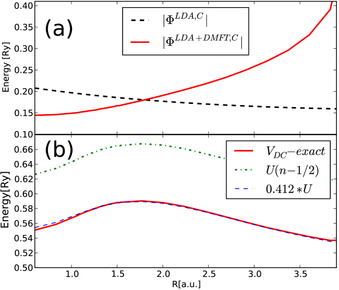
Figure 2: (Color online) (a) Correlation energy of LDA and LDA+DMFT versus interatomic separation in H₂ molecule. The DMFT correlation is evaluated by $\Phi^{\mathrm{LDA+DMFT},C}=\Phi^{\mathrm{LDA},C}+\sum_{i}E^{\mathrm{DMFT},i}-\sum_{i}\Phi^{DC}[\rho^{i}_{local}]$, where potential energy $E^{\mathrm{DMFT},i}=\frac{1}{2}{\mathrm{Tr}}(\Sigma^{i}_{loc}{\cal G}^{i}_{loc})$. (b) LDA+DMFT double-counting potential $V_{DC}$ versus $R$, which is defined as the functional derivative of $\Phi^{DC}[\rho^{i}_{local}]$ given in Eq. 3.

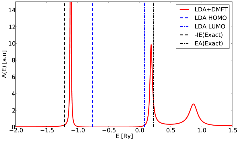
Figure 3: (Color online) LDA+DMFT spectral function (red) presented with the HOMO and LUMO energy of LDA (blue), and the exact $-$IE and EA (black).

To gain deeper insight into correlation energy, we plot in Fig. 2 the correlated energy of the LDA and LDA+DMFT versus ion separation. The LDA correlation energy slightly decreases with increasing distance Baerends (2001) in contrast to physical expectations. On the other hand, the LDA+DMFT correlation is small when the two ions are close, and it increases sharply with increasing distance, signaling a Mott-like transition, where we find the DMFT self-energy develops a non-analytic pole between highest occupied molecular orbital (HOMO) and lowest unoccupied molecular orbital (LUMO).

In the lower panel of Fig. 2, the exact double-counting potential within LDA+DMFT defined as $V_{DC}=\bra{\chi_{i}}\delta\Phi^{DC}/\delta\rho^{i}_{local}\ket{\chi_{i}}$ versus $R$ is displayed. The often used phenomenological form $U(n-1/2)$, first introduced in the context of LDA+U Anisimov et al. (1997), is also shown for comparison. The exact double-counting is kept somewhat smaller than the phenomenological form, and its variation is almost entirely due to variation of local Coulomb repulsion $U=\bra{\chi_{i}\chi_{i}}U_{C}(\textbf{r}-\textbf{r}^{\prime})\ket{\chi_{i}\chi_{i}}$, with proportionality constant $V_{DC}\approx 0.412U$. In the solid state calculations, the self-consistent form of the double-counting $U(n-1/2)$ is also often found too large and is many times reduced (see discussion in Ref. Haule et al., 2014.)

In Fig. 3, we plot the LDA+DMFT spectral function at equilibrium distance R = 1.4, which has been analytically continued to the real axis by Pade method. The highest occupied quasi-particle peak (HOMO, below 0) has the physical meaning of minus the ionization energy ($-\mathrm{IE}=E_{H_{2}}-E_{H_{2}^{+}}$) while the lowest unoccupied peak (LUMO, above 0) corresponds to electron affinity ($\mathrm{EA}=E_{H_{2}^{-}}-E_{H_{2}}$). These quantities are called vertical IE and vertical EA, respectively, because these energies of removal/addition of an electron are calculated with fixed interatomic separation R. The exact $-$IE ($-1.207$ Ry) and EA (0.224 Ry) are presented as black vertical lines, calculated from the total energy difference using the exact methods Hadinger et al. (1989); Kolos and Wolniewicz (1964); Srivastava et al. (2012). We also mark the position of LDA HOMO ($-0.754$ Ry) and LDA LUMO (0.084 Ry) with blue lines.

The LDA HOMO is almost 40% off the $-\mathrm{IE}$ and the LDA LUMO is around 60% off the EA. This failure of Kohn-Sham (KS) eigenvalues is due to delocalization error of LDA functional, connected with the well known underestimation of band-gaps by LDA Zhan et al. (2003); Zhang and Musgrave (2007). On the other hand, the spectral function of LDA+DMFT, in which the KS eigenvalues are renormalized by DMFT self-energy, shows a sharp resonance around $-1.110$ Ry (7% of error bar), a substantial improvement from 40% error bar of LDA HOMO. The LUMO peak is also refined from $0.084$ Ry (LDA) to $0.192$ Ry which is only 0.032 Ry off the exact value.

Although LDA+DMFT spectral function considerably improves the LDA excitations, it still deviates from the exact result (for $-$IE, it is about 7% off). In order to obtain an insight into this mismatch of the LDA+DMFT spectral function and the exact result, we investigated H₂ in two different ways using GW-RPA approach: (a) one considering GW correlation in the entire Hilbert space and (b) the other where GW is solely confined to the DMFT projected space (Eq (II)). Firstly, we found no significant total energy difference ($\sim 0.005Ry$) between two schemes. On the other hand, for spectral function, the scheme (a) yields its $-$IE peak very close to the exact value within 0.1% error while that of the scheme (b), in which GW correlation is restricted to the minimal DMFT orbitals, is also 7% off the exact $-$IE peak. This indicates that the correlation of the rest of the Hilbert space needs to be included to predict an accurate spectra of H₂ although the correlation within the minimal orbital set (Eq. (II)) is enough to capture the total energy precisely. We believe that multi-orbital LDA+DMFT framework, where the DMFT correlations are also extended to higher excited states of the system, would lead to progressively better results.

IV Conclusion

In summary, a good implementation of LDA+DMFT with a high-quality projector and exact double-counting that have been introduced here, can rival many quantum chemistry methods in its precision. In the DMFT case, since the most time consuming part of the method – the inclusion of correlations on a given ion – scales linearly with the system size, it holds great promise in future quantum chemistry and solid state applications, although it still needs to be tested in other molecular systems to establish its ultimate usefulness in quantum chemistry applications. We have showed that the H₂ molecule is a very good testing ground for electronic structure methods addressing correlation problem, especially because the screening effects are not obscuring problems connected with the choice of the functional to be minimized. The present methodology will be useful in further developing other electronic structure methods such as GW+DMFT, where the precise form of the functional, the level of self-consistency, screening, and double-counting still need to be adequately addressed.

*

Appendix A The double-counting functional in detail

We firstly define the projected local Green’s function for the $i$-th atom using the DMFT projector $\ket{\chi_{i}}$ (Eq. (II)):

$$G^{i}(\omega)=\bra{\chi_{i}}G(\omega)\ket{\chi_{i}}$$ (4)

where the index $i$ specifies the atomic site $L$ or $R$ and in position space it takes the form of

$${\cal G}^{i}(\omega;\textbf{r},\textbf{r}^{\prime})=\chi_{i}(\textbf{r})G^{i}(i\omega)\chi_{i}^{*}(\textbf{r}^{\prime}).$$ (5)

For more complete model, we define projectors containing orbital index $\alpha$ as well as the site index $i$, $\ket{\chi_{\alpha}^{i}}$, which is relevant for molecules with heavier atoms. The local Green’s function in DMFT basis is then written as $G^{i}_{\alpha\alpha^{\prime}}=\bra{\chi_{\alpha}^{i}}G(\omega)\ket{\chi_{\alpha^{\prime}}^{i}}$ and its position space version is ${\cal G}^{i}(\textbf{r},\textbf{r}^{\prime})=\sum_{\alpha,\alpha^{\prime}}\chi_{\alpha}^{i}(\textbf{r})G^{i}_{\alpha\alpha^{\prime}}\chi_{\alpha^{\prime}}^{i*}(\textbf{r}^{\prime})$.

The Luttinger-Ward functional for LDA+DMFT approximation is

$$\Phi^{LDA+DMFT} =$$ (6)

$$\sum_{i}\Phi^{DMFT} [G^{i}_{local}]+\Phi^{LDA}[\rho]-\sum_{i}\Phi^{DC}[\rho^{i}_{local}].$$

Here the local density $\rho^{i}_{local}$ is defined in the same way as ${\cal G}^{i}(\textbf{r},\textbf{r}^{\prime})$ from $G(\textbf{r},\textbf{r}^{\prime})$, namely,

$$\rho^{i}_{local}(\textbf{r}) =\chi_{i}(\textbf{r})n^{i}_{local}\chi_{i}^{*}(\textbf{r})$$ (7)

where $n^{i}_{local}$ is local occupation.

The double-counting energy can be split into Hartree-Fock part $\Phi^{DC}_{HF}$ and the correlation part $\Phi^{DC}_{c}$. The Hartree-Fock part is straightforward to evaluate in DMFT basis as

$$\Phi^{DC}_{HF}[\rho^{i}_{local}]=\frac{1}{2} \sum_{\sigma\sigma^{\prime}}\bra{\chi_{i}\chi_{i}}U_{C}\ket{\chi_{i}\chi_{i}}\times$$ (8)

$$(n^{i}_{local,\sigma}n^{i}_{local,\sigma^{\prime}}-\delta_{\sigma\sigma^{\prime}}n^{i}_{local,\sigma}n^{i}_{local,\sigma}).$$

When a single orbital per site is considered with the above defined projector, the Hartree-Fock energy and potential simplify to

$$\Phi^{DC}_{HF}[\rho^{i}_{local}]=\frac{1}{4}U_{local}(n^{i}_{local})^{2}$$ (9)

$$V^{DC}_{HF}[\rho^{i}_{local}]\equiv\frac{\delta\Phi^{DC}_{HF}[n^{i}_{local}]}{\delta n^{i}_{local}}=\frac{1}{2}U_{local}n^{i}_{local}$$ (10)

where $U_{local}=\bra{\chi_{i}\chi_{i}}U_{C}\ket{\chi_{i}\chi_{i}}$ is the local Coulomb matrix element. When multiple orbitals are considered by DMFT, the Hartree-Fock double counting term generalizes to $\Phi^{DC}_{HF}=\frac{1}{2}\sum_{\alpha\beta\gamma\delta,\sigma\sigma^{\prime}}\bra{\chi_{i\alpha}\chi_{i\beta}}U_{C}\ket{\chi_{i\gamma}\chi_{i\delta}}(n^{\sigma}_{\alpha\delta}n^{\sigma^{\prime}}_{\beta\gamma}-\delta_{\sigma\sigma^{\prime}}n^{\sigma}_{\alpha\gamma}n^{\sigma}_{\beta\delta})$. where $\alpha\beta\gamma\delta$ run over active orbitals on a given atom.

The double-counting for correlation energy within LDA+DMFT we propose here is

$$\Phi^{DC}_{c}[\rho^{i}_{local}]=\int_{\textbf{r}}\varepsilon^{LDA}_{c}(\rho^{i}_{local}(\textbf{r}),U_{C})\rho^{i}_{local}(\textbf{r})$$ (11)

This is exactly DMFT approximation of LDA correlation functional, truncating $G(\textbf{r},\textbf{r}^{\prime})\rightarrow{\cal G}^{i}(\textbf{r},\textbf{r}^{\prime})$ that yields $\rho(\textbf{r})\rightarrow\rho^{i}_{local}(\textbf{r})$. The expression $\varepsilon^{LDA}_{c}(\rho^{i}_{local}(\textbf{r}),U_{C})$ in Eq. (11) implies that it is a functional of both density and Coulomb interaction $U_{C}(\textbf{r},\textbf{r}^{\prime})=\frac{2}{|\textbf{r}-\textbf{r}^{\prime}|}$. In solid state, we should replace $U_{C}(\textbf{r},\textbf{r}^{\prime})$ with a screened one ${\cal U}^{\lambda}_{C}(\textbf{r},\textbf{r}^{\prime})=\frac{2e^{-\lambda|\textbf{r}-\textbf{r}^{\prime}|}}{|\textbf{r}-\textbf{r}^{\prime}|}$ and therefore we need to obtain the LDA correlation functional with respect to two parameters $\rho$ and $\lambda$ for exact double counting. In small molecular systems such as H₂ screening effect is negligible (${\cal U}^{\lambda}_{C}(\textbf{r},\textbf{r}^{\prime})\approx U_{C}(\textbf{r},\textbf{r}^{\prime})$) and therefore the functional form of the LDA correlation $\varepsilon^{LDA}_{c}$ in double-counting (11) is intact.

The double counting potential $V^{i}_{DC}$ in the DMFT basis can be easily computed:

$$V^{i}_{DC} \equiv\frac{\delta\Phi^{DC}_{c}[\rho^{i}_{local}]}{\delta n^{i}_{local}}$$

$$=\int_{\textbf{r}}|\chi_{i}(\textbf{r})|^{2}V_{c}^{LDA}[\rho^{i}_{local}(\textbf{r})]$$ (12)

where $V_{c}^{LDA}$ is the LDA correlation potential that takes the form of $V_{c}^{LDA}\equiv\varepsilon_{c}^{LDA}+\delta\varepsilon_{c}^{LDA}/\delta\rho$. In derivation, we used the relation (7) and the chain rule. In more general case with multiple local degrees of freedom, the form of local density (7) should be replaced with $\rho_{local}(\textbf{r})=\sum_{\alpha,\alpha^{\prime}}\chi_{\alpha}^{i}(\textbf{r})\rho^{i}_{\alpha\alpha^{\prime}}\chi_{\alpha^{\prime}}^{i*}(\textbf{r})$ where $\rho^{i}_{\alpha\alpha^{\prime}}=\bra{\chi_{\alpha}^{i}}\hat{\rho}\ket{\chi_{\alpha^{\prime}}^{i}}$ is projected density matrix onto site $i$.

References

- Hohenberg and Kohn (1964) P. Hohenberg and W. Kohn, Phys. Rev. 136, B864 (1964).
- Kohn and Sham (1965) W. Kohn and L. J. Sham, Phys. Rev. 140, A1133 (1965).
- Georges and Kotliar (1992) A. Georges and G. Kotliar, Phys. Rev. B 45, 6479 (1992).
- Georges et al. (1996) A. Georges, G. Kotliar, W. Krauth, and M. J. Rozenberg, Rev. Mod. Phys. 68, 13 (1996).
- Kotliar and Vollhardt (2004) G. Kotliar and D. Vollhardt, Physics Today 57, 53 (2004).
- Kotliar et al. (2006) G. Kotliar, S. Y. Savrasov, K. Haule, V. S. Oudovenko, O. Parcollet, and C. A. Marianetti, Rev. Mod. Phys. 78, 865 (2006).
- Lin et al. (2011) N. Lin, C. A. Marianetti, A. J. Millis, and D. R. Reichman, Physical Review Letters 106, 096402 (2011).
- Zgid and Chan (2011) D. Zgid and G. K.-L. Chan, J. Chem. Phys. 134, 094115 (2011).
- Jacob et al. (2010) D. Jacob, K. Haule, and G. Kotliar, Phys. Rev. B 82, 195115 (2010).
- Turkowski et al. (2012) V. Turkowski, A. Kabir, N. Nayyar, and T. S. Rahman, J. Chem. Phys. 136, 114108 (2012).
- Anisimov et al. (1997) V. Anisimov, F. Aryasetiawan, and A. I. Lichtenstein, J. Phys.: Condens. Matter 9, 767 (1997).
- Haule et al. (2014) K. Haule, T. Birol, and G. Kotliar, Phys. Rev. B 90, 075136 (2014).
- Dang et al. (2014) H. T. Dang, A. J. Millis, and C. A. Marianetti, Phys. Rev. B 89, 161113 (2014).
- Stollhoff and Fulde (1977) G. Stollhoff and P. Fulde, Zeitschrift für Physik B Condensed Matter 26, 257 (1977).
- Stollhoff and Fulde (1978) G. Stollhoff and P. Fulde, Zeitschrift für Physik B Condensed Matter 29, 231 (1978).
- Hadinger et al. (1989) G. Hadinger, M. Aubert-Frecon, and G. Hadinger, J. Phys. B: At., Mol. Opt. Phys. 22, 697 (1989).
- Paul and Kotliar (2006) I. Paul and G. Kotliar, Eur. Phys. J. B 51, 189 (2006).
- Haule et al. (2010) K. Haule, C.-H. Yee, and K. Kim, Phys. Rev. B 81, 195107 (2010).
- Marzari and Vanderbilt (1997) N. Marzari and D. Vanderbilt, Phys. Rev. B 56, 12847 (1997).
- Pavarini et al. (2004) E. Pavarini, S. Biermann, A. Poteryaev, A. I. Lichtenstein, A. Georges, and O. K. Andersen, Phys. Rev. Lett. 92, 176403 (2004).
- Anisimov et al. (2005) V. I. Anisimov, D. E. Kondakov, A. V. Kozhevnikov, I. A. Nekrasov, Z. V. Pchelkina, J. W. Allen, S.-K. Mo, H.-D. Kim, P. Metcalf, S. Suga, A. Sekiyama, G. Keller, I. Leonov, X. Ren, and D. Vollhardt, Phys. Rev. B 71, 125119 (2005).
- Amadon et al. (2008) B. Amadon, F. Lechermann, A. Georges, F. Jollet, T. O. Wehling, and A. I. Lichtenstein, Phys. Rev. B 77, 205112 (2008).
- Werner and Millis (2006) P. Werner and A. J. Millis, Phys. Rev. B 74, 155107 (2006).
- Haule (2007) K. Haule, Phys. Rev. B 75, 155113 (2007).
- Baym and Kadanoff (1961) G. Baym and L. P. Kadanoff, Phys. Rev. 124, 287 (1961).
- Baym (1962) G. Baym, Phys. Rev. 127, 1391 (1962).
- Vosko et al. (1980) S. H. Vosko, L. Wilk, and M. Nusair, Canadian Journal of Physics 58, 1200 (1980).
- Gunnarsson et al. (1989) O. Gunnarsson, O. Andersen, O. Jepsen, and J. Zaanen, Phys. Rev. B 39, 1708 (1989).
- Aryasetiawan et al. (2004) F. Aryasetiawan, M. Imada, A. Georges, G. Kotliar, S. Biermann, and A. Lichtenstein, Phys. Rev. B 70, 195104 (2004).
- Kolos and Wolniewicz (1964) W. Kolos and L. Wolniewicz, J. Chem. Phys. 41, 3663 (1964).
- Stan et al. (2009) A. Stan, N. E. Dahlen, and R. van Leeuwen, J. Chem. Phys. 130, 114105 (2009).
- Baerends (2001) E. J. Baerends, Phys. Rev. Lett. 87, 133004 (2001).
- Srivastava et al. (2012) S. Srivastava, N. Sathyamurthy, and A. Varandas, Chemical Physics 398, 160 (2012).
- Zhan et al. (2003) C.-G. Zhan, J. A. Nichols, and D. A. Dixon, J. Phys. Chem. A 107, 4184 (2003).
- Zhang and Musgrave (2007) G. Zhang and C. B. Musgrave, J. Phys. Chem. A 111, 1554 (2007).