Predicting Excitonic Gaps of Semiconducting Single Walled Carbon Nanotubes From a Field Theoretic Analysis

Abstract

We demonstrate that a non-perturbative framework for the treatment of the excitations of single walled carbon nanotubes based upon a field theoretic reduction is able to accurately describe experiment observations of the absolute values of excitonic energies. This theoretical framework yields a simple scaling function from which the excitonic energies can be read off. This scaling function is primarily determined by a single parameter, the charge Luttinger parameter of the tube, which is in turn a function of the tube chirality, dielectric environment, and the tube’s dimensions, thus expressing disparate influences on the excitonic energies in a unified fashion. We test this theory explicitly on the data reported in NanoLetters 5, 2314 (2005) and Phys. Rev. B. 82, 195424 (2010) and so demonstrate the method works over a wide range of reported excitonic spectra.

One of the most challenging problems in studying low dimensional strongly correlated systems is the quantitative prediction of the absolute values of the energies of its fundamental excitations. These energies are typically non-perturbative in nature and so lie out of the reach of approximations that treat interactions as weak. One non-perturbative theoretical tool that is not so limited is quantum field theory. Quantum field theories arise as descriptions of condensed matter systems by focusing on their low energy properties. They have had considerable success in studying a number of problems in quantum magnetism Dender ; Oshi ; Essler ; Essler1 ; Essler2 ; spinladders ; Oshi1 , in particular the remarkable prediction of an $E_{8}$ symmetry in a critical quantum Ising model in a longitudinal field Zamo that has been recently observed Coldea , one dimensional Mott insulator physics Tsvelik ; Tsvelik1 ; SO(8)ladder ; Hubbard , and Luttinger liquids in all of their various forms quantumwires ; egger ; kane1 ; smitha ; helicaledgestates ; luttingerjunction ; levtsv . However quantum field theories are best at predicting universal properties of materials. Typically they do not attempt to understand absolute values of gap energies, but instead are satisfied with (the still very non-trivial task of) computing ratios of excitation energies.

In this letter we show that this restriction need not always hold. We demonstrate that the data that can be extracted from a field theoretic analysis can in fact be used to predict the absolute magnitude of excitation gaps. To this end we analyze a field theoretic treatment of the excitonic spectra of semi-conducting carbon nanotubes konik . The excitonic gaps of semiconducting carbon nanotubes are known to be both variegated, depending on tube diameter, chirality, subband, and dielectric environment sfeir_nano ; bnl_nano ; wang ; Bachilo ; 3+4 ; flu ; rmp . They are also known to be strongly renormalized by Coulomb interactions from their bare, non-interacting values ando ; kane ; wang ; louie ; vasily . Both of these features make them an ideal testing ground for the analysis presented herein.

Typically excitonic spectra of carbon nanotubes have been determined using a Bethe-Salpeter equation combined with first principle input louie ; vasily ; vasily1 ; molinari ; louie1 . While this methodology results in an estimate for the absolute magnitude of an excitonic gap, it does so by focusing upon a particular subband of a tube of a particular chirality and in a particular dielectric environment. In our field theoretic treatment of excitonic spectra, even though we are interested in the absolute values of gaps, we are still able to derive a universal scaling function from which the values of the excitonic gaps can be read off. The key parameter of this scaling function will be the total charge Luttinger parameter, $K_{c+}$, a measure of the effective strength of Coulomb interactions in the tube egger ; kane .

We begin our field theoretical treatment by focusing on a single subband of a carbon nanotube. It is straightforward to argue that intersubband interactions lead only to very weak perturbations on the spectra of a single subband epaps . To describe this subband at low energies we introduce four sets (two for the spin, $\sigma$, degeneracy and two for the valley, $\alpha=K,K^{\prime}$, degeneracy) of right ($r=+$) and left ($r=-$) moving fermions, $\psi_{r\alpha\sigma}$. The Hamiltonian governing these fermions can be written as $H=\int dx({\cal H}_{kin}+{\cal H}_{gap})+H_{Coulomb}$. ${\cal H}_{kin}+{\cal H}_{gap}$ together give the non-interacting band dispersion, $\epsilon^{2}(p)=v_{0}^{2}p^{2}+\Delta_{0}^{2}$:

$${\cal H}_{kin}=-iv_{0}\psi^{\dagger}_{r\alpha\sigma}\partial_{x}\psi_{r\alpha\sigma};~{}~{}{\cal H}_{gap}=\Delta_{0}\psi^{\dagger}_{r\alpha\sigma}\psi_{-r\alpha\sigma},$$ (1)

where $v_{0}$ is the bare velocity of the fermions and repeated indices are summed. For the Coulombic part of the Hamiltonian we only consider the strongest part of the forward scattering term:

$$H_{Coulomb}=\frac{1}{2}\int dxdx^{\prime}\rho(x)V_{0}(x-x^{\prime})\rho(x^{\prime}),$$

where $\rho(x)=\sum_{r\alpha\sigma}\psi^{\dagger}_{r\alpha\sigma}(x)\psi_{r\alpha\sigma}(x)$. The remaining Coulombic terms only affect the excitonic gaps at the $1\%$ level.

A unique feature of our theoretical approach is that we take into account the Coulomb interactions at the start of the analysis. In particular, instead of treating $H_{Coulomb}$ as a perturbation of $\int dx({\cal H}_{kin}+{\cal H}_{gap})$, we treat $\int dx{\cal H}_{gap}$ as a perturbing term of $\int dx{\cal H}_{kin}+H_{Coulomb}$. The “unperturbed” Hamiltonian is nothing more than the Hamiltonian of a metallic carbon nanotube while ${\cal H}_{gap}$ is treated as a confining interaction on top of the metallic tube. To proceed in this fashion works because we can treat $\int dx{\cal H}_{kin}+H_{Coulomb}$ exactly using bosonization.

If we bosonize $H_{0}$ in terms of chiral bosons $\phi_{r\alpha\sigma}$ by writing $\psi_{r\alpha\sigma}\sim\exp(i\phi_{r\alpha\sigma})$, we arrive at a simple result kane1 ; egger . The theory is equivalent to four Luttinger liquids described by the four bosons $\theta_{i}$, $i=c_{\pm},s_{\pm}$ (and their duals $\phi_{i}$)

$$H_{0}=\int dx\sum_{i}\frac{v_{i}}{2}\bigg{(}K_{i}(\partial_{x}\phi_{i})^{2}+K_{i}^{-1}(\partial_{x}\theta_{i})^{2}\bigg{)}.$$ (2)

The four bosons diagonalizing $H_{0}$ are linear combinations of the original four bosons and represent an effective charge-flavour separation where $\theta_{c+}=\sum_{r\alpha\sigma}r\tilde{\psi}_{r\alpha\sigma}$ is the charge boson and the remaining three bosons reflect the spin, valley, and parity symmetries in the problem. The charge boson is the only boson to see the effects of the Coulomb interaction. Both the charge Luttinger parameter, $K_{c+}$, and the charge velocity, $v_{c+}=v_{0}/K_{c+}$, are strongly renormalized. We make note here that $K_{c+}$ is the key parameter and will be the one by which we organize all of our results.

For long range Coulomb interactions, $K_{c+}$ takes the form

$$K_{c+}=\bigg{(}1+\frac{8e^{2}}{\pi\kappa\hbar v_{0}}\big{(}-\log(k_{\rm min}R)+c_{0}\big{)}\bigg{)}^{-1/2},$$ (3)

where $\kappa$ is the dielectric constant of the medium surrounding the tube, $k_{\rm min}$ is minimum allowed wavevector in the tube, $R$ is the tube’s radius, and $c_{0}$ is a wrapping vector dependent $O(1)$ constant smitha ; egger . $k_{\rm min}$ necessarily has to be larger than $2\pi/L$ where $L$ is the length of the tube, but can in principle be much larger, say on the order of the inverse mean free path in the tube. In typical nanotubes $K_{c+}$ can take on values in the range of $\sim.2$. The remaining Luttinger parameters, $K_{i}$, $i=c_{-},s_{\pm}$ retain their non-interacting values, $1$, and so their velocities, $v_{i}=v_{0}$ go unrenormalized.

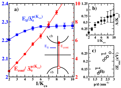
Figure 1: a) The scaling functions (see Eqns. 6 and 7) for the $E_{ii}$ excitons and the particle-hole continuum, $E_{cont}$. At $K_{c+}=1$ (the non-interacting limit) these functions go to $2$. Inset to a) Sketch of $E_{ii}$ and $E_{cont}$ excitations. b) The function $A(K_{c+})$ giving the size of the finite bandwidth correction to $E_{ii}$. c) The size of this correction, $\delta E_{exc}$, for the excitons, $E_{44}$ and $E_{55}$, of the four tubes studied in Ref.bnl_nano .

Under bosonization ${\cal H}_{gap}$ becomes

$${\cal H}_{gap}=\frac{4\tilde{\Delta}_{0}}{\pi}(\prod_{i}\cos(\frac{\theta_{i}}{2})+\prod_{i}\sin(\frac{\theta_{i}}{2})),$$ (4)

where $\tilde{\Delta}_{0}=\Delta_{0}(\Lambda/v_{c+})^{(1-K_{c+})/4}$ and $\Lambda$ is the bandwidth of the tube. This renormalization of the bandwidth has important consequences for the excitonic physics of the tube. In field theoretic language, the coupling $\Delta_{0}$, has picked up an anomalous dimension. Rather than purely having the dimensions of energy, $\tilde{\Delta}_{0}$ now has the dimensions of ${\rm energy}^{(5-K_{c+})/4}\times{\rm velocity}^{(K_{c+}-1)/4}$. This means that all excitations gaps of the tube no longer linearly scale with $\tilde{\Delta}_{0}$ but scale rather with the non-trivial power $\tilde{\Delta}_{0}^{4/(5-K_{c+})}$. Coupling constants (here the bare gap) inheriting “anomalous dimensions” is a standard feature of quantum field theories. These anomalies allow one to easily access aspects of non-perturbative physics: an immediate consequence of this was argued in Ref. konik to be that the ratio of excitons between the first and second subbands goes as $2^{4/(5-K_{c+})}$ (not 2 as predicted by non-interacting band theory), so providing a straightforward resolution of what Ref. kane termed the exciton ratio problem.

While this explanation of the ratio problem required no information of how the cutoff, $\Lambda$, depends on the tube parameters, we need more to be able to make quantitative predictions of the exciton gaps in any given tube. $\Lambda$ reflects the largest energy scale in the low energy reduction of the tube. This energy scale is not the bandwidth of graphene ($\sim 9$eV), but rather some much smaller scale reflecting that the electrons on the tubes are delocalized around the tube’s circumference. We thus take as an ansatz

$$\frac{\Lambda}{v_{c+}}=\frac{B}{d},$$ (5)

where $B$ is an $O(1)$ dimensionless constant and $d=2R$ is the tube’s diameter. We cannot directly determine this constant, but treat it as a fitting parameter, the only undetermined parameter of this approach. But we will see the same constant works over tubes with a wide variety of radii, different subbands within the same tube, and tubes in different dielectric environments. We will also see, as an important self-consistency check, that this same relation determines the finite bandwidth corrections to the excitonic gaps of higher subbands.

To this end the gap, $E_{\alpha}$, of any excitation $\alpha$ (exciton, single particle, or otherwise) takes the following universal scaling form

$$E_{\alpha}=f^{\Lambda}_{\alpha}(K_{c+})\tilde{\Delta}_{0}^{4/(5-K_{c+})}v_{c+}^{\mu(K_{c+})},$$ (6)

with $\mu(K_{c+})=(1-K_{c+})/(5-K_{c+})$ and where $f^{\Lambda}_{\alpha}(K_{c+})$ is a scaling function. It takes the form

$$f^{\Lambda}_{\alpha}(K_{c+})\!=\!f^{\infty}_{\alpha}(K_{c+})\big{(}1\!+\!A(K_{c+})(\frac{\tilde{\Delta}_{0}}{v_{0}})^{2}(\frac{v_{0}}{\Lambda})^{\frac{5-K_{c+}}{2}}\big{)}.$$ (7)

$f^{\infty}_{\alpha}(K_{c+})$ governs the gap in the large bandwidth, $\Lambda\gg\Delta_{0}$, limit and was already determined in konik . However not previously considered, the scaling function sees corrections at finite bandwidth. These corrections will be important for predicting accurately the excitonic gaps of excitons in the higher subbands. The constant $A(K_{c+})$ is a dimensionless parameter (but depends on the charge Luttinger parameter) that governs the size of these corrections. It is plotted in Fig. 1b. The form of $A(K_{c+})$ is derived in Ref. epaps .

To extract the scaling function $f^{\Lambda}(K_{c+})$, we numerically study the full Hamiltonian, ${\cal H}_{0}+{\cal H}_{gap}$, using a truncated conformal spectrum approach (TCSA) zamo combined with a Wilsonian renormalization group kon1 . The results for the scaling functions for the optically active excitons, $E_{ii}$, and the particle-hole continuum, $E_{cont}$, are shown in Fig. 1a as a function of $K_{c+}$. We see the scaling function for $E_{ii}$ is relatively flat as a function of $K_{c+}$ while that of $E_{cont}$ varies comparatively sharply. In the limit $K_{c+}$ tends to 1 (the non-interacting limit), the scaling function $f^{\infty}_{ii}$ tends to 2 (i.e. the exciton energy is that of the bare (non-interacting) particle-hole continuum gap). In the limit $K_{c+}$ tends to 0, $f^{\infty}_{ii}\propto K_{c+}^{-1/5}$, only going to infinity slowly. In contrast, $f^{\infty}_{cont}$, grows much more quickly, going as $K_{c+}^{-1}$. We have thus quantified the general observation kane that the renormalization of the single particle gap due to Coulomb interactions is much more marked than that of the excitons. It is also much stronger than has been suggested in RPA-type computations Ando . We also immediately infer that the binding energy of the exciton as a fraction of the exciton energy grows as $K_{c+}^{-4/5}$ as $K_{c+}\rightarrow 0$.

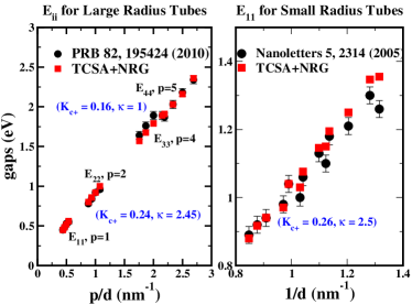
Figure 2: Left: Comparison of the measured exciton gaps of the first four subbands, $E_{ii}$, $i=1,2,3,4$ ($p=1,2,4,5$ in the notation of Ref. kane ), reported in Ref. bnl_nano of four nanotubes with different chiralities with gaps derived from the scaling function determined by NRG+TCSA. Right: Same comparison but the measured excitonic gaps are of the first subband, $E_{11}$, in a set of small radius tubes as reported in Ref. sfeir_nano .

Analysis of Experimental Data: We now examine how this theoretical approach fares in predicting the excitonic data of Refs. bnl_nano and sfeir_nano . These papers present excitonic gaps of tubes for a wide range of diameters and subbands as well as different dielectric environments. This will allow us to test the flexibility of the above theoretical scheme.

In Ref. bnl_nano measurements were performed on a set of four larger diameter tubes (d running from 1.86nm to 2.14nm). In each of the four tubes, the first four single photon excitons, $E_{ii}$, $i=1,\cdots,4$, were measured. $E_{33}$ and $E_{44}$ were studied by suspending the nanotubes and using Rayleigh scattering spectroscopy. In these measurements the relevant dielectric constant was $\kappa=1$. These same tubes were then printed onto a silicon wafer where source and drain electrons were patterned. This enabled $E_{11}$ and $E_{22}$ to be measured by a complimentary technique, Fourier-transform photoconductivity. In this configuration the effective dielectric constant of the tubes is the average of air and silicon dioxide, $\kappa=(1+\kappa_{\rm SiO_{2}})/2=2.45$, a result easily derived from considering the effective potential between two charges confined to the interface of two media with different dielectric constants. To determine the appropriate value of the Luttinger parameter for these tubes, we need to specify $k_{min}$. The length, $L$, of the tubes of Ref. bnl_nano was typically $L\sim 2\mu$ (a number equal to the mean free path mft ) and so we take $k_{min}=2\pi/l$. This leads to a Luttinger parameter of $K_{c+}=0.16$ for the tubes suspended in air and $K_{c+}=0.24$ for the tubes printed onto the silicon substrate. The smaller $K_{c+}$ for the suspended tubes indicates the action of a considerably stronger effective Coulomb interactions for the tubes in this configuration.

In Ref. sfeir_nano the single photon excitons, $E_{11}$, were measured for a set of 13 tubes with diameters between 0.78nm and 1.18nm. The tubes were embedded in a polymaleic acid/octyl vinyl ether (PMAOVE) matrix with an effective dielectric constant of $\kappa$=2.5 wang . The excitons were measured using two photon spectroscopy – thus the $E_{2g}$ photons were also studied in this work but will not be considered here. As the length of tubes in the PMAOVE matrix was reported to be $L=400$nm columbia , far smaller than $l_{mf}$, we take $k_{min}=2\pi/L$ here. This leads to a Luttinger parameter of $K_{c+}=0.26$. Because of the logarithmic dependence of $K_{c+}$ upon $k_{min}$, $K_{c+}$ is relatively insensitive to ${\cal O}(1)$ changes of $k_{min}$.

As an ingredient to our analysis of the data in Refs. bnl_nano ; sfeir_nano we need to determine the bare value of the gap, $\Delta_{0}$, for each tube. We do so with a tight binding model based on wrapping a honeycomb lattice of nearest neighbor spacing $a_{0}=1.42$A^o and hopping parameter $t=3.0$eV. We do not attempt to include curvature, twist, or stress corrections to $\Delta_{0}$ (eggert ; yang ) although for small radius tubes such corrections may not be insignificant. But to be able to do so would require detailed characterization of the tubes in their environment which is not available. As we have explained the treatment has one fitting parameter: the constant $B$ governing the relationship between the effective bandwidth of the nanotube and the tube’s diameter, $d$. To find this constant $B$ we focus on the four $E_{11}$ excitonic gaps reported in bnl_nano . We focus on these gaps because for these the correction due to finite bandwidth (the second term in Eqn. 7) can safely be ignored. When we fit Eqn. (5) we find $B\sim 0.51$. We will henceforth use this value for B to determine theoretical values of the gaps for all the other single photon excitons reported in Refs. bnl_nano ; sfeir_nano .

Remarkably this relationship between the bandwidth and the tube’s diameter leads to excellent values for the other excitonic gaps considered in this study. To demonstrate this we first consider all (16) of the gaps reported in Ref. bnl_nano . Our results for the gaps are presented in Table 1 of Ref. epaps and Fig. 2a. We see that the agreement between the theoretically predicted values of the gaps and the corresponding experimentally measured values is less than $2\%$ for the $E_{11}$, $E_{22}$, $E_{44}$, and one of the $E_{33}$ gaps and on the order of $5\%$ for the remaining $E_{33}$ gaps. The relatively good agreement found for the $E_{33}$ and $E_{44}$ gaps is a result of taking into account the finite bandwidth corrections coming from the subleading term in Eqn. (7) where the corrections for $E_{33}$ and $E_{44}$ are large ($>100$ meV – see Fig. 1c). These corrections in Eqn. (7), inasmuch as they are proportional to $\tilde{\Delta}_{0}^{2}/\Lambda^{(5-K_{c+})/2}$, depend in turn upon our identification of $\Lambda$ with the tube diameter. It is an important consistency check for this ansatz in Eqn. (5) that the computed corrections lead to a good match between the experiment and theory.

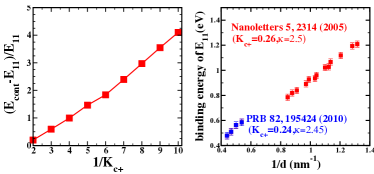
Figure 3: Left: Binding energy of exciton expressed in units of the excitonic gap. Right: The predicted binding energies of the excitonic gaps, $E_{11}$, reported in Refs. bnl_nano ; sfeir_nano .

We find similar good agreement in our theoretical analysis of the $E_{11}$ excitons reported in Ref. bnl_nano . Using the same relationship of the bandwidth, we plot our predicted values for $E_{11}$ against those measured in Ref. sfeir_nano in Fig. 3. We see that only for the three smallest radius tubes do we not obtain excellent agreement between theory and experiment (as explained earlier a likely consequence of missing curvature, strain, and twist effects on the bare gap, $\Delta_{0}$). It is important to stress that the same value of $B$ derived from the four $E_{11}$ large radius tube gaps in Ref. bnl_nano leads to an accurate prediction of the gaps for the smaller radius tubes in Ref. sfeir_nano .

Excitonic Binding Energies: We finally consider the excitonic binding energies of the $E_{11}$ excitons reported in Refs. bnl_nano ; sfeir_nano . We first plot in Fig. 3a the excitonic binding energies as a function of $K_{c+}^{-1}$. The binding energies are presented as a fraction of the exciton gap. We see that for $K_{c+}^{-1}$ large, the binding energies can be many multiples of the excitonic gap itself. As $K_{c+}^{-1}$ decreases, the fractional exciton binding energy decreases linearly in line with the linear decrease of $E_{cont}$ (as seen in Fig. 1a). In Fig. 3b we plot the excitonic binding energies for the $E_{11}$ excitons. Given that $K_{c+}^{-1}\sim 4$ for these gaps, we see that from Fig. 3a the binding energies roughly equal the gaps, $E_{11}$, themselves. The estimates of the binding energies for the $E_{11}$ excitons of Ref. sfeir_nano are considerably larger than those in Ref. louie1 , a consequence of our much larger estimate here of the renormalized band gaps. It would thus be of considerable interest if these band gaps could be measured directly. But this is a difficult task as the standard method for measuring the particle-hole continuum, scanning tunneling microscopy lin , involves placing the tubes on a metallic substrate. The consequent screening of the Coulomb interaction leads to values of $K_{c+}$ near to 1, far away from values of $K_{c+}$ appropriate for the excitons measured in Ref. bnl_nano ; sfeir_nano .

In summary, we have presented a quantum field theoretical formalism able to predict the absolute magnitudes of optically active excitons in semi-conducting carbon nanotubes over a wide range of diameters, subbands, and dielectric environments. This method involves a single fitting parameter, $B$, relating the effective bandwidth of the tube to the tube’s diameter. Once this parameter is in hand, a simple scaling function yields the excitonic gaps for arbitrary nanotubes. We have compared the predictions of this formalism with the excitonic data of Refs. bnl_nano ; sfeir_nano and have found good agreement.

I Acknowledgements

The research herein was carried out in part in the CMPMS Dept. (RMK and JM) and at the Center for Functional Nanomaterials (MS), Brookhaven National Laboratory, which is supported by the U.S. Department of Energy, Office of Basic Energy Sciences, under Contract No. DE-AC02-98CH10886.

II Supplementary Material

II.1 Tables Comparing Measured Excitonic Gaps with Theoretical Predictions

We report in Tables 1 and 2 the data for the excitons measured in Ref. bnl_nano and Ref. sfeir_nano .

(n,m)	$K_{c+},i=1,2$	$\Delta_{0,11}$	$E_{11,Th}$	$E_{11,Exp}$	$\Delta_{0,22}$	$E_{22,Th}$	$E_{22,Exp}$	$K_{c+},i=3,4$	$\Delta_{0,33}$	$E_{33,Th}$	$E_{33,Exp}$	$\Delta_{0,44}$	$E_{44,Th}$	$E_{44,Exp}$
(14,13)	0.241	0.232	0.56	0.55	0.466	1.00	0.96	0.156	0.913	1.89	1.89	1.139	2.36	2.34
(19,14)	0.244	0.190	0.45	0.45	0.377	0.80	0.78	0.158	0.759	1.57	1.64	0.921	1.91	1.87
(17,12)	0.242	0.216	0.52	0.53	0.427	0.92	0.92	0.157	0.863	1.79	1.89	1.039	2.16	2.18
(18,13)	0.243	0.202	0.48	0.48	0.400	0.86	0.84	0.158	0.808	1.68	1.76	0.977	2.03	2.03

Table 1: Comparison of the experimental and theoretical values of $E_{ii}$ of the large radius tubes reported in Ref. bnl_nano . All energies in units of eV.

(n,m)	$K_{c+}$	$\Delta_{0,11}$	$E_{11,Th}$	$E_{11,Exp}$
(8,3)	0.26	0.562	1.35	1.30
(6,5)	0.26	0.564	1.36	1.26
(7,5)	0.26	0.523	1.25	1.21
(10,2)	0.26	0.499	1.20	1.18
(9.4)	0.26	0.478	1.15	1.13
(7,6)	0.26	0.479	1.15	1.1
(8,6)	0.26	0.448	1.08	1.06
(11,3)	0.26	0.434	1.04	1.04
(9,5)	0.26	0.436	1.03	1.00
(8,7)	0.26	0.416	0.97	0.98
(9,7)	0.26	0.392	0.94	0.94
(12,4)	0.26	0.383	0.92	0.92
(11,6)	0.26	0.367	0.88	0.89

Table 2: Comparison of the experimental and theoretical values of $E_{11}$ of the small radius tubes reported in Ref. sfeir_nano .

II.2 Derivation of the Scaling Function Governing the Excitonic Gaps

In order to derive the form of the scaling function in Eqn. (7), we need to first understand how a cutoff, which we will call $\Lambda_{TCSA}$, is implemented in the numerical methodology, the TCSA+NRG konik , used to study this system. This method is able to study any Hamiltonian which can be written as a perturbed conformal field theory:

$${\cal H}={\cal H}_{CFT}+\lambda\Phi_{\rm perturbation},$$ (8)

where here in this case ${\cal H}_{CFT}$ is a theory of four bosons, $\theta_{i}$, the coupling $\lambda$ equals $4\tilde{\Delta}_{0}/\pi$, and $\Phi_{\rm perturbation}=(\prod_{i=1}^{4}\cos(\theta_{i}/2)+\prod_{i=1}^{4}\sin(\theta_{i}/2))$. The method uses the Hilbert space of ${\cal H}_{CFT}$ as a computational basis. (For details see Refs. konik ; kon1 .) This computational basis is optimal because the exact computation of matrix elements of $\Phi_{\rm perturbation}$ is readily done using the commutation relations of the governing algebra of the unperturbed conformal theory, the Virasoro algebra. Being able to compute these matrix elements means ${\cal H}$ can be recast as a matrix. For this matrix to be a finite matrix, we need to truncate the Hilbert space of ${\cal H}_{CFT}$. The unperturbed energies of the eigenstates of ${\cal H}_{CFT}$, $\{|\beta\rangle\}$, appearing in the excitonic sector have the form

$$E_{\beta}=\sum_{i=1}^{4}\frac{v_{0}}{K_{i}}(\frac{2\pi n_{i}}{R}-\frac{c}{12}),$$ (9)

where the $n_{i}$ are integers and $c$ is the central charge of a single boson ($c=1$). To implement the cutoff we then insist that the integers, $n_{i}$, satisfy $\sum_{i}(n_{i}/K_{i})\leq N$. This allows us to define the cutoff of this method as

$$\Lambda_{TCSA}=v_{0}\frac{2\pi N}{R}.$$ (10)

With this in hand, the next step in the derivation of the scaling form is to write down the $\beta$-function of the coupling constant $\tilde{\Delta}$:

$$N\frac{d\tilde{\Delta}_{0}}{dN}=\alpha(K_{c+})\frac{\tilde{\Delta}_{0}^{3}}{v_{0}^{2}}\bigg{(}\frac{R}{2\pi N}\bigg{)}^{(5-K_{c+})/2}.$$ (11)

In principle $\alpha(K_{c+})$ can be determined analytically – we however extract it numerically from the TCSA data. This numerical determination is what is used to plot $A(K_{c+})$ in Fig. 1b. The form this $\beta$-function has can be determined following Ref. Watts by insisting that the partition function of the theory remains invariant under changes in the cutoff $N$. In the gapped phase of the theory with $R$ sufficiently large this is equivalent to insisting the gaps of the theory are invariant under the RG flow.

If we integrate this $\beta$-function we obtain an expression relating the coupling in the absence of a cutoff to that with a cutoff:

$$\tilde{\Delta}_{0}(N=\infty)=\frac{\tilde{\Delta}_{0}(N)}{1-\frac{4\alpha(K_{c+})}{5-K_{c+}}\frac{\tilde{\Delta}_{0}^{2}(N)}{v_{0}^{2}}(\frac{R}{2\pi N})^{(5-K_{c+})/2}}.$$ (12)

The gaps, $E_{\alpha}$, in the absence of a cutoff, depend on the coupling $\tilde{\Delta}_{0}(\infty)$ via the relation,

$$E_{\alpha}(N=\infty,\tilde{\Delta}_{0}=\tilde{\Delta}_{0}(\infty))=f^{\infty}_{\alpha}\tilde{\Delta}_{0}(\infty)^{4/(5-K_{c+})},$$ (13)

a simple consequence of dimensional analysis (taking into account the anomalous dimensions of the coupling constant, $\tilde{\Delta}_{0}$). By RG invariance we have $E_{\alpha}(N=\infty,\tilde{\Delta}(\infty))=E_{\alpha}(N,\tilde{\Delta}(N))$. So substituting this into Eqn. 13 and using Eqn. 12 we obtain the desired scaling form:

$$E_{\alpha}(N,\tilde{\Delta}_{0}(N)) = f^{\infty}_{\alpha}(\tilde{\Delta}_{0}(N))^{4/(5-K_{c+})}\times$$ (16)

$$\hskip-72.26999pt\bigg{(}1+\frac{16\alpha(K_{c+})}{(5-K_{c+})^{2}}(\frac{\tilde{\Delta}_{0}}{v_{0}})^{2}(\frac{R}{2\pi N})^{(5-K_{c+})/2}\bigg{)}.$$

The only issue is that this is expressed in terms of the TCSA cutoff $\Lambda_{TCSA}=2\pi N/R$ that arises from our numerical treatment of the problem and not the effective bandwidth of the tube, $\Lambda$.

To determine the relationship between $\Lambda$ and $\Lambda_{TCSA}$ we begin by consider the bosonization formula giving the right/left moving fermion, $\psi^{\dagger}_{\pm}$, in terms of a normal ordered vertex operator of a boson:

$$\psi^{\dagger}_{\pm}(x)\sim:e^{i\phi_{\pm}(x)}\!:.$$ (17)

In writing this expression we have dropped prefactors, zero modes, and Klein factors – for our purposes what matters is the normal ordered exponential. The key to the relationship between $\Lambda$ and $\Lambda_{TCSA}$ is found in the relation between the normal ordered vertex operator and its unnormal ordered counterpart:

$$:e^{i\phi(x)}\!: = \sqrt{\frac{2\pi}{R}}e^{i\phi_{\pm}(x)}e^{\frac{1}{2}\sum^{N}_{n>0}\frac{1}{n}}$$ (18)

$$\approx \sqrt{\frac{2\pi}{L}}e^{i\phi_{\pm}(x)}e^{\gamma/2}N^{1/2},$$ (20)

where $\gamma$ is the Euler constant and the factor $\sqrt{2\pi/L}$ ensures the engineering dimension of the normal ordered vertex operator matches its anomalous dimension. The appearance of $N=R\Lambda_{TCSA}/2\pi$ reflects our use of the TCSA cutoff to regulate the UV divergences that normal ordering exhibits in the theory.

When we initially bosonize the theory, the total charge boson is normal ordered assuming $K_{c+}=1$. When we rediagonalize the theory, absorbing the forward scattering part of the Coulomb interaction into the quadratic part of ${\cal H}$, we have to adjust the normal ordering to take into account $K_{c+}\neq 1$. We do so as follows:

$$:e^{\theta_{c+}/2}\!:_{K_{c+}=1} = (\frac{2\pi}{R})^{1/4}e^{\gamma/4}N_{c}^{1/4}e^{i\theta_{c+}/2}$$

$$= \bigg{(}e^{\gamma}\frac{2\pi N_{c}}{R}\bigg{)}^{(1-K_{c+})/4}:e^{\theta_{c+}/2}\!:_{K_{c+}\neq 1},$$

where the subscripts $::_{K_{c+}}$ indicate the value of $K_{c+}$ for which the normal ordering is being done. We use $N_{c}$ instead of $N$ as $N_{c}$ governs the maximal energy in the total charge (c+) sector of the theory, not the entire theory itself. The two are related via

$$N_{c+}=\frac{Nv_{0}}{4v_{c+}},$$ (23)

assuming an equipartition of energy between the four bosons in the theory. It is this difference in normal ordering prefactors that is absorbed into the bare coupling:

$$\tilde{\Delta}_{0}=\Delta_{0}\bigg{(}e^{\gamma}\frac{2\pi N_{c+}}{R}\bigg{)}^{(1-K_{c+})/4}.$$ (24)

This then implies (comparing the above with the relation below Eqn. (4) in the main body of the text)

$$\frac{\Lambda}{v_{c+}}=\frac{e^{\gamma}}{4v_{c+}}\Lambda_{TCSA}=\frac{B}{d}.$$ (25)

With this relation, we can now place the scaling function into its final form, Eqn. (7), substituting $\Lambda$ for $\Lambda_{TSCA}$ in Eqn. (16).

II.3 Corrections to Excitonic Energies due to Intersubband Interactions

In this section we will compute the corrections to excitonic energies due to interactions between subbands. We will demonstrate that they are proportional to $v_{F}^{4}/c^{4}$ where $c$ is the speed of light and so is small.

Consider an excitonic excitation in subband i with energy $\Delta_{i}$. The forward scattering portion of the intersubband Coulomb interaction (as with the intrasubband interactions, the strongest part of the Coulomb interaction) takes the form

$$H_{\rm interCI}=\sum_{i>j}\int dxdx^{\prime}\rho_{i}(x)V_{c}(x-x^{\prime})\rho_{j}(x^{\prime})$$ (26)

where $\rho_{i}$ is the density in the $i-$th subband. In the long wavelength limit this can be rewritten as

$$H_{\rm interCI} = \sum_{i>j}\int dx\rho_{i}(x)\rho_{j}(x)V_{c}(k=0)$$ (27)

$$= \Gamma\sum_{i>j}\int dx\partial_{x}\theta_{c+,i}(x)\partial_{x}\theta_{c+,j}(x),$$ (29)

where $\Gamma=v_{F}/(8\pi K_{c+})$ and we have used in the second line the bosonized expressions for the electron densities in the subbands.

In second order perturbation theory the correction to $\Delta_{i}$ takes the form

$$\delta\Delta_{i}=\Gamma^{2}\sum_{n}\frac{|\langle\Delta_{i}|\otimes\langle GS_{j}|H_{\rm interCI}|GS_{i}\rangle\otimes|\Delta_{n,j}\rangle|^{2}}{\Delta_{i}-\Delta_{n,j}}$$ (30)

where $|\Delta_{n,j}\rangle$ is some excitation in the $j-$th subband with parity odd symmetry (i.e. odd under $\theta_{c+,j}\rightarrow-\theta_{c+,j}$) with energy $\Delta_{n,j}$. The lowest energy such excitations are the one-photon excitons in subband $j$. The state $|GS_{j}\rangle$ is the ground state of the $j-$th subband. The matrix elements that we to evaluate in this sum take the form

$$\langle\Delta_{i}|\rho_{i}(x)|GS_{i}\rangle = M_{i}e^{ip_{i}x}p_{i};$$ (31)

$$\langle\Delta_{n,j}|\rho_{j}(x)|GS_{j}\rangle = M_{n,j}e^{ip_{j}x}p_{j,n},$$ (33)

where $M_{i}$ and $M_{n,j}$ are ${\cal O}(1)$ constants (as can be verified numerically) and $p_{i}/p_{n,j}$ are the momenta of the excitations $|\Delta_{i}\rangle$/$|\Delta_{n,j}\rangle$. Thus the energy correction takes the form

$$\delta\Delta_{i}=\sum_{n}\frac{v_{F}^{2}p_{1}^{4}|M_{i}|^{2}|M_{j,n}|^{2}\Gamma^{2}}{(\Delta_{i}^{2}+v_{F}^{2}p_{i}^{2})(\Delta_{i}-E_{n,j})}.$$ (34)

As one can see this correction vanishes as the momentum of the exciton goes to zero. Typically the momentum of an optically excited exciton will be equal to $\Delta_{i}/c$, implying that $\delta\Delta_{i}$ is proportional to $(v_{F}/c)^{4}$ and so is very small.

References

- (1) D. C. Dender, P. R. Hammar, D. H. Reich, C. Broholm, and G. Aeppli, Phys. Rev. Lett. 79, 1750 (1997).
- (2) M. Oshikawa and I. Affleck, Phys. Rev. Lett. 79, 2883 (1997); I. Affleck and M. Oshikawa, Phys. Rev. B 60, 1038 (1999).
- (3) F. H. L. Essler, Phys. Rev. B 59 14376 (1999).
- (4) I. Kuzmenko and F. H. L. Essler, Phys. Rev. B 79 024402 (2009).
- (5) F. H. L. Essler and R. M. Konik, Phys. Rev. B 75, 144403 (2007); R. M. Konik, F. H. L. Essler, and A. M. Tsvelik, Phys. Rev. B 78, 214509 (2008).
- (6) F. H. L. Essler, A. M. Tsvelik, and G. Delfino, Phys. Rev. B 56, 11001 (1997).
- (7) S. C. Furuya and M. Oshikawa, Phys. Rev. Lett. 109, 247603 (2012).
- (8) A. B. Zamolodchikov, Int. J. Mod. Phys. A 4, 4235 (1989).
- (9) R. Coldea, D. A. Tennant, E. M. Wheeler, E. Wawrzynska, D. Prabhakaran, M. Telling, K. Habicht, P. Smeibidl, and K. Kiefer, Science 327, 177 (2010).
- (10) F. H. L. Essler and A. M. Tsvelik, Phys. Rev. B 65, 115117 (2002).
- (11) F. H. L. Essler and A. M. Tsvelik, Phys. Rev. Lett. 88, 096403 (2002).
- (12) H. H. Lin, L. Balents, and M.P.A. Fisher, Phys. Rev. B 58, 1794 (1998); R. M. Konik and A. W. W. Ludwig, Phys. Rev. B 64, 155112 (2001).
- (13) M. J. Bhaseen, F. H. L. Essler, and A. Grage, Phys. Rev. B 71, 020405 (2005).
- (14) L.S. Levitov, A.M. Tsvelik, Phys. Rev. Lett. 90, 016401 (2003).
- (15) C.L. Kane and M.P.A. Fisher, Phys. Rev. B 46, 15233 (1992).
- (16) Chang-Yu Hou, Eun-Ah Kim, and Claudio Chamon, Phys. Rev. Lett. 102, 076602 (2009).
- (17) A. Agarwal, S. Das, S. Rao, and D. Sen, Phys. Rev. Lett. 103 026401 (2009); A. Rahmani, C.-Y. Hou, A. Feiguin, M. Oshikawa, C. Chamon, and I. Affleck, Phys. Rev. B 85, 045120 (2012).
- (18) W. DeGottardi, T.-C. Wei, and S. Vishveshwara, Phys. Rev. B 79, 205421 (2009).
- (19) R. Egger and A. O. Gogolin, Eur. Phys. J. B 3, 281 (1998).
- (20) C. L. Kane, L. Balents, and M. P. A. Fisher, Phys. Rev. Lett. 79, 5086 (1997).
- (21) R. M. Konik, Phys. Rev. Lett. 106, 136805 (2011).
- (22) M. Y. Sfeir, J. A. Misewich, S. Rosenblatt, Y. Wu, C. Voisin, H. Yan, S. Berciaud, T. F. Heinz, B. Chandra, R. Caldwell, Y. Shan, J. Hone, and G. L. Carr, Phys. Rev. B 82, 195424 (2010).
- (23) G. Dukovic, F. Wang, D. Song, M. Y. Sfeir, T. Heinz, and L. Brus, Nanoletters 5, 2314 (2005).
- (24) A. Kleiner and S. Eggert, Phys. Rev. B 63, 073408 (2001).
- (25) L. Yang, M. P. Anantram, J. Han, and J. P. Lu, Phys. Rev. B 60, 13874 (1999).
- (26) F. Wang, G. Dukovic, L. E. Brus, T. F. Heinz, Science 308, 838 (2005).
- (27) S. M. Bachilo, M. S. Strano, C. Kittrell, R. H. Hauge, R. E. Smalley, R. B. Weisman, Science 298, 2361 (2002).
- (28) P. T. Araujo, S. K. Doorn, S. Kilina, S. Tretiak, E. Einarsson, S. Maruyama, H. Chacham, M. A. Pimenta, and A. Jorio, Phys. Rev. Lett. 98, 067401 (2007).
- (29) M. J. O’Connell, S. M. Bachilo, C. B. Huffman, V. C. Moore, M. S. Strano, E. H. Haroz, K. L. Rialon, P. J. Boul, W. H. Noon, C. Kittrell, J. Ma, R. H. Hauge, R. B. Weisman, and R. E. Smalley, Science 297, 593 (2002).
- (30) J.-C. Charlier, X. Blase, and S. Roche, Rev. Mod. Phys. 79, 677 (2007).
- (31) T. J. Ando, Phys. Soc. Jpn. 1997, 66, 1066
- (32) M. Rohlfing and S.G. Louie, Phys. Rev. B 62, 4927 (2000).
- (33) V. Perebeinos, , J. Tersoff, and P. Avouris, Phys. Rev. Lett. 92, 257402 (2004).
- (34) V. Perebeinos, J. Tersoff, and P. Avouris, Nano Lett. 5, 2495 (2005).
- (35) J. Maultzsch, R. Pomraenke, S. Reich, E. Chang, D. Prezzi, A. Ruini, E. Molinari, M. S. Strano, C. Thomsen, and C. Lienau, Phys. Rev. B 72, 241402(R) (2005); D. Kammerlander, D. Prezzi, G. Goldoni, E. Molinari, and U. Hohenester, Phys. Rev. Lett. 99, 126806 (2007).
- (36) J. Deslippe, M. Dipoppa, D. Prendergast, M. V. O. Moutinho, R. B. Capaz, S. G. Louie, Nano Lett. 9, 1330 (2009).
- (37) C.L. Kane, E.J. Mele, Phys. Rev. Lett. 93, 197402 (2004).
- (38) V. P. Yurov and Al. B. Zamolodchikov, Int. J. Mod. Phys. A 6, 4557 (1991).
- (39) R. M. Konik and Y. Adamov, Phys. Rev. Lett. 98, 147205 (2007).
- (40) H. Sakai, H. Suzuurab, T. Ando, Physica E 22, 704 (2004).
- (41) G. Dukovic, B. E. White, Z. Zhou, F. Wang, S. Jockusch, M. L. Steigerwald, T. F. Heinz, R. A. Friesner, N. J. Turro, and L. E. Brus, J. Am. Chem. Soc. 126, 15269 (2004).
- (42) M. S. Purewal, B. H. Hong, A. Ravi, B. Chandra, J. Hone, and P. Kim, Phys. Rev. Lett. 98, 186808 (2007).
- (43) H. Lin, J. Lagoute, V. Repain, C. Chacon, Y. Girard, J.-S. Lauret, F. Ducastelle, A. Loiseau, and S. Rousset, Nature Materials 9, 235 (2010).
- (44) R. M. Konik, M. Y. Sfeir, and J. M. Misewich, supplementary material.
- (45) G. Watts, Nucl. Phys. B 859, 177 (2012); P. Giokas and G. Watts, arXiv:1106.2448.