The role of metallicity in high mass X-ray binaries in galaxy formation models

Abstract

Context. Recent theoretical works claim that high-mass X-ray binaries could have been important sources of energy feedback into the interstellar and intergalactic media, playing a major role in both the early stages of galaxy formation and the physical state of the intergalactic medium during the reionization epoch. A metallicity dependence of the production rate or luminosity of the sources is a key ingredient generally assumed but not yet probed.

Aims. Our goal is to explore the relation between the X-ray luminosity and star formation rate of galaxies as a possible tracer of a metallicity dependence of the production rates and/or X-ray luminosities of high-mass X-ray binaries, using hydrodynamical cosmological simulations.

Methods. We developed a model to estimate the X-ray luminosities of star forming galaxies based on stellar evolution models which include metallicity dependences. We applied our X-ray binary models to galaxies selected from hydrodynamical cosmological simulations which include chemical evolution of the stellar populations in a self-consistent way. Hence for each simulated galaxies we have a distribution of stellar populations with different ages and chemical abundances, determined by its formation history. This allows us to robustely predict the X-ray luminosity – star formation rate relation under different hypotheses for the effects of metallicity.

Results. Our models successfully reproduce the dispersion in the observed relations as an outcome of the combined effects of the mixture of stellar populations with heterogeneous chemical abundances and the metallicity dependence of the X-ray sources. We find that the evolution of the X-ray luminosity as a function of the star formation rate of galaxies could store information on possible metallicity dependences of the high-mass X-ray sources. A non-metallicity dependent model predicts a non-evolving relation while any metallicity dependence should affect the slope and the dispersion as a function of redshift. Our results suggest the characteristics of the X-ray luminosity evolution can be linked to the nature of the metallicity dependence of the production rate or the X-ray luminosity of the stellar sources. By confronting our models with current available observations of strong star-forming galaxies, we find that only chemistry-dependent models reproduce the observed trend for $z<4$. However, it is is not possible to prove the nature of this dependence yet.

1 Introduction

High-mass X-ray binaries (HMXBs) are systems composed by a compact object, which can be a neutron star (NS) or a black hole (BH), and an early-type star. The compact object accretes mass from its companion star, converting gravitational into thermal energy, part of which is radiated away in the X-ray band ($\sim 0.1-10\ {\rm keV}$). Since the first high-energy observatories (Einstein, ROSAT, ASCA), these sources have been observed in the Milky Way as well as in nearby galaxies. In the last decade, the higher angular resolution and sensitivity of Chandra and XMM-Newton allowed these observatories to detect thousands of HMXBs in the local Universe (Grimm et al. 2003; Fabbiano 2006; Mineo et al. 2012, and references therein). The relation between HMXBs and massive stars makes these sources dominate the X-ray luminosity of star-forming galaxies with high specific star formation rate (sSFR). Mineo et al. (2012) have compiled a large sample of HMXBs in nearby late-type galaxies, for which they claim that the contamination by other types of sources (i.e. low-mass X-ray binaries —LMXBs—, background active galactic nuclei) is negligible. Recently, the X-ray emission of a sample of metal-poor blue compact dwarf galaxies was investigated by Kaaret et al. (2011), and different authors have studied the properties of X-ray emitting star-forming galaxies at high redshift (Cowie et al. 2012; Basu-Zych et al. 2013). These observations have provided a large amount of data on the properties of HMXB populations, and on the relation of these properties to those of the host galaxies.

HMXBs are an important tool to investigate stellar (particularly binary) evolution, and the nature of compact objects. They are also potential star-formation tracers due to their relation to massive stars, and they have been proposed as important sources of stellar energy feedback into the interstellar and intergalactic media (Power et al. 2009; Mirabel et al. 2011; Dijkstra et al. 2012; Justham & Schawinski 2012; Power et al. 2013). One of the key problems to understand these systems, their evolution, and their influence on the environment, is the dependence of the HMXB production and properties on the metallicity of the stellar populations from which they form. Recent stellar evolution models suggest that the number of BHs and NSs produced by a stellar population depends on its metallicity (Georgy et al. 2009). Binary population synthesis models show that also the fraction of these compact objects that end up in binary systems with massive companions should depend on metallicity (Belczynski et al. 2004b; Dray 2006; Belczynski et al. 2008, 2010b; Linden et al. 2010), because at lower metallicities more systems can survive disruption when the primary BH forms, and also avoid merging in the common-envelope phase. Finally, both models and observations suggest that low-metallicity stars form more massive BHs, which could produce potentially higher-luminosity HMXBs (Belczynski et al. 2010a; Linden et al. 2010; Feng & Soria 2011, and references therein).

However, the observational evidence for the metallicity dependence of the number and luminosity function of HMXBs is still poor. It is clear that this dependence must be searched for in the properties of the populations of HMXBs in star-forming galaxies. A key observable is the X-ray luminosity $L_{\rm X}$ of such galaxies, which in the local Universe scales with the star formation rate (SFR; Grimm et al. 2003; Mineo et al. 2012). This correlation is usually parameterized as $L_{\rm X}=3.5\times 10^{40}{\rm erg}\ {\rm s}^{-1}\ f_{\rm X}\ {\rm SFR}/(M_{\odot}\ {\rm yr}^{-1})$, where the factor $f_{\rm X}$ accounts for possible variations due to the dependence of HMXB properties on metallicity or other physical parameters. Mineo et al. (2012) found that observations of nearby galaxies are consistent with a constant $f_{\rm X}\sim 0.2$, but the correlation shows a large dispersion, which might be due to metallicity effects. Kaaret et al. (2011) measured unusually larger $f_{\rm X}$ values for a sample of nearby blue compact dwarf galaxies with low metallicities. Unfortunately, their small sample did not allow them to reach statistically meaningful conclusions about a departure of these galaxies from the standard $L_{\rm X}$–SFR relation of Grimm et al. (2003). Cowie et al. (2012) investigated this issue using a sample of galaxies at high redshift, for which metallicity effects should be important due to the chemical evolution of the Universe. They found that $f_{\rm X}$ is at most marginally dependent on redshift, however the observational uncertainties and the complex dependence of galaxy metallicity on redshift still leave the question open. Using the same X-ray survey Basu-Zych et al. (2013) have studied Lyman-Break galaxies in the range $z=1.5-8$, finding instead that $f_{\rm X}$ evolves with redshift. They also argue that Cowie et al. (2012) did not correct the galaxy luminosities for dust attenuation, which could prevent them to observe the evolution. A key issue to resolve the problem is to understand how $f_{\rm X}$ is affected by the metallicity dispersion within a galaxy, the correlation of the galaxy mean metallicity and SFR, and the chemical evolution of the Universe, in order to make a proper interpretation of the observational results.

An interesting way to explore the metallicity dependence of HMXB populations, and the key issue of the possible evolution of $f_{\rm X}$, is through the combination of binary population synthesis models with a description of the stellar populations in a galaxy. Belczynski et al. (2004a) used this method to develop models that reproduce the emission of specific galaxies, while Zuo & Li (2011) explored the X-ray emission of galaxies at different redshifts using prescriptions for their star formation histories. These authors found a good agreement between the predicted and observed X-ray luminosity to stellar mass ratio in the range $z=0-4$, but they were not able to reproduce the corresponding X-ray to optical luminosity ratio. A step forward in this approach is to couple binary population synthesis models to scenarios for the formation and evolution of galaxies in a cosmological context. Previous works used population synthesis models which provide a description of the HMXB properties expected from a single, homogeneous parent stellar population or semi-analytical models where there is a unique mean metallicity for stellar populations born at a certain time in a given galaxy. As we mentioned before, we intent to improve the modeling of HMXBs by providing a more realistic description of the complexity of stellar populations within a galaxy.

Here we present a novel scheme to model the HMXB populations of star-forming galaxies, which couples population synthesis results to galaxy catalogues constructed from a hydrodynamical cosmological simulation of structure formation which is part of the Fenix project (Tissera et al., in prep.). This simulation includes star formation, a multiphase treatment of the interstellar medium, the chemical enrichment of baryons, and the feedback from supernovae in a self-consistent way (Scannapieco et al. 2005, 2006), and reproduces global dynamical and chemical properties of galaxies (de Rossi et al. 2010; De Rossi et al. 2012; Pedrosa et al. 2014). This makes the simulation well suited for the task of investigating the evolution of the $L_{\rm X}$–SFR relation of star forming galaxies, expanding and complementing the results obtained by other methods such as semi-analytical models (e.g., Fragos et al. 2013a). Our scheme is similar to those applied by Nuza et al. (2007), Chisari et al. (2010), Artale et al. (2011), and Pellizza et al. (2012) to the study of gamma-ray bursts. It includes both the modelling of the intrinsic HMXB populations of galaxies, and the definition of different samples comparable to observations, based on the modelling of selection effects. This is an important ability of our scheme, as it allows us to make a fair comparison with observations to constrain free parameters and discard incorrect hypotheses. Using our scheme, we develop different models to explore the effects of the dependence of the HMXB population properties on the metallicity of the parent stellar populations, and address the question of the evolution of the $f_{\rm X}$ factor by comparing our predictions to observations of galaxies across time.

This paper is organized as follows. In Section 2 we briefly present the numerical simulations used to describe the formation and evolution of galaxies, and the construction of galaxy catalogues. In Section 3 we describe our HMXB model and how it is implemented onto the simulated galaxy catalogues to generate intrinsic population. In Section 4, we present our results as a function of cosmic time. Finally, in Section 5, we discuss our main conclusions.

2 Simulations

The simulation used in this work (S230A) is part of the Fenix project (Pedrosa et al. 2014), designed to study the role of metals in galaxy formation (Tissera et al., in prep.). The run was performed with a version of GADGET-3 (Springel 2005) which includes star formation, metal-dependent cooling, chemical enrichment, a multiphase model for the interstellar medium, and supernovae feedback (Scannapieco et al. 2005, 2006).

The feedback model includes Type II and Type Ia supernovae (SNII and SNIa, respectively) for chemical and energy production, within a multiphase model for the interstellar medium. The SN feedback model considers as progenitors of SNII stars with masses larger than $8\,M_{\odot}$ and assumes lifetimes of $\approx 10^{6}\,{\rm yr}$. The lifetimes of SNIa are selected randomly within the range $0.1-1\,{\rm Gyr}$. A constant ratio between the rates of SNII and SNIa is assumed. In the analysed simulation the thermal energy released into the interstellar medium per SN event is $0.7\times 10^{51}\,{\rm erg}$. The chemical algorithm from Mosconi et al. (2001) was adapted for GADGET-2 by Scannapieco et al. (2005), with initial primordial abundances for gas particles of $X_{\rm H}=0.76$ and $X_{\rm He}=0.24$. The algorithm follows the enrichment of 12 isotopes: ¹H, ²He, ¹²C, ¹⁶O, ²⁴Mg, ²⁸Si, ⁵⁶Fe, ¹⁴N, ²⁰Ne, ³²S, ⁴⁰Ca and ⁶²Zn. The chemical yields for SNII are taken from Woosley & Weaver (1995) while for SNIa, we adopt the W7 model of Thielemann et al. (1993). The SN feedback model used in S230A has proven to be successful at regulating the star formation activity, and at driving powerful mass-loaded galactic winds without the need to introduce mass-dependent parameters.

The simulation S230A describes a cubic volume of $10h^{-1}\,{\rm Mpc}$ per side, consistent with a $\Lambda$-CDM universe with cosmological parameters $\Omega_{\Lambda}=0.7$, $\Omega_{\rm m}=0.3$, $\Omega_{\rm b}=0.04$, $\sigma_{8}=0.9$, and ${\rm H}_{0}=100h\,{\rm km}\,{\rm s}^{-1}\,{\rm Mpc}^{-1}$, where $h=0.7$. Initially the simulation has $2\times 230^{3}$ particles in total, with masses of $8.47\times 10^{6}\,M_{\odot}$ for dark matter and $1.3\times 10^{6}\,M_{\odot}$ for gas particles. S230A has been used by de Rossi et al. (2010) and De Rossi et al. (2012) to study the Tully-Fisher relation, obtaining good agreement with observations. Furthermore, the evolution of the dark matter halo mass function as a function of redshift reproduces that obtained from the Millenium Simulation (De Rossi et al. 2013). Nevertheless we acknowledge the fact that this simulation overproduces the stellar mass formed at high redshift which is an ubiquitous problem for $\Lambda$-CDM scenarios. In fact, in a forthcoming paper we will explore how HMBXs might contribute to solve this problem.

The virialized structures were selected by using a friends-of-friends technique and the substructures within their virial radii were identified with the SUBFIND algorithm (Springel et al. 2001). Galaxy catalogues were constructed from $z\sim 0$ to $z\sim 5$ by selecting those substructures with more than 3000 particles, which is equivalent to have galaxies with stellar masses above $\sim 10^{8}\,M_{\odot}$. For each simulated galaxy we have the chemical abundances and ages of its stellar populations. The mass-metallicity relation (MZR) of galaxies in the simulation was studied by de Rossi et al. (2010), finding a lower mean metallicity for a fixed stellar mass than that observed by Tremonti et al. (2004). Hence, we renormalized the simulated abundances adopting the results from Maiolino et al. (2008) to make them consistent with current observational results.

Each of the simulated galaxies is formed by a combination of stellar populations spatially distributed according to its formation history. The new-born stars have different chemical abundances and it is from these mixed stellar populations that the progenitors of HMXBs are chosen. To illustrate this point, in Fig.  1 we show the stellar mass fractions as a function of metallicity ($Z$) and of age for one of the simulated galaxies, for different redshifts. Metallicity is defined as the ratio between the total mass in chemical elements heavier than He and the stellar mass of a given stellar population. Each analysed galaxy has more than 1000 star particles which represent its stellar populations. These distributions vary for galaxies with diferent assembly histories. This is one of the major advantage of using hydrodynamical cosmological simulations. A drawback of our model it is that we have simplified scheme for HMXBs compared to those of Fragos et al. (2013a), for example. However, each approach can contribute with a different insight to a given problem and it is from the complementary findings that deeper knowledge might be achieved.

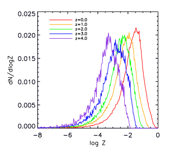
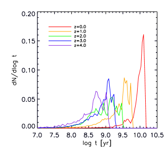
Figure 1: Mass fraction of the stellar populations as a function of metallicity (Z, upper panel) and age (lower panel) for a typical galaxy. The distributions are displayed for different redshifts. At each available time, HMXB progenitors are selected from these stellar populations by following constrains on age and metallicity described in the following sections.

3 Population synthesis

3.1 The HMXB population of a galaxy

For each simulated galaxy, we produce a synthetic HMXB population using the properties of its stellar populations (i.e., the metallicities and ages of more than a few thousands of particles describing them). Given that the progenitors of HMXBs are massive stars, the compact objects in these systems form shortly after a star formation episode. Both theoretical models (Belczynski et al. 2008) and observations (Shtykovskiy & Gilfanov 2007) suggest that the X-ray emission peaks roughly 20–40 Myr after the starburst. Hence, we assume that only young stellar populations will contribute with HMXBs, and select only those stellar populations with ages lower than 100 Myr. Our results do not depend strongly on the particular choice of this value, as far as its order of magnitude is preserved.

We compute the number of NS and BHs produced by each stellar population selected from the galaxy catalogues, according to the model of Georgy et al. (2009) for the evolution of massive stars. This model includes stellar rotation and the dependence of the type of compact remnant on the metallicity of the progenitor star. An important feature of this model is the prediction of a higher fraction of BHs as the metallicity decreases. For a stellar population $p$ with mass $m_{*,p}$ and metallicity $Z$, formed at redshift $z_{p}$, we calculate the number of BHs and NS as

$$N^{\rm BH,NS}_{p}=m_{*,p}\frac{\int_{R^{\rm BH,NS}(Z)}\xi(m)dm}{\int^{100\,M_{\odot}}_{0.1\,M_{\odot}}m\xi(m)dm},$$ (1)

where $R^{\rm BH,NS}(Z)$ defines the mass range over which each type of compact remnant is produced at metallicity $Z$, $\xi(m)$ is the Salpeter (1955) initial mass function (IMF) with lower and upper mass cut-offs of $0.1\,M_{\odot}$ and $100\,M_{\odot}$, respectively. This choice of IMF is consistent with that implemented in the analysed numerical cosmological simulation.

A fraction $f_{\rm bin}^{\rm BH,NS}$ of the progenitors of these compact objects belongs primordial binaries, and a fraction $f_{\rm rem}^{\rm BH,NS}$ of these binaries remains bound after the supernova event in which the compact objects are produced. A fraction $f_{\rm HM}^{\rm BH,NS}$ of these X-ray binaries will have high-mass companions. Finally, only a fraction $f_{\rm acc}^{\rm BH,NS}$ of these will be in the X-ray binary phase (i.e., accreting matter from the companion and emitting X-rays) at any time. Hence, the ratio of the number of emitting HMXBs to that of the compact objects produced by the stellar population is

$$f_{\rm HMXB}^{\rm BH,NS}=f_{\rm bin}^{\rm BH,NS}f_{\rm rem}^{\rm BH,NS}f_{\rm HM}^{\rm BH,NS}f_{\rm acc}^{\rm BH,NS}.$$ (2)

Then, the number of HMXB systems produced in each stellar population in our galaxy catalogues is

$$N_{{\rm HMXB},p}=f^{\rm BH}_{\rm HMXB}\,N^{\rm BH}_{p}+f^{\rm NS}_{\rm HMXB}\,N^{\rm NS}_{p},$$ (3)

and the number of HMXBs in each galaxy $g$ is

$$N_{\rm HMXB}=\sum_{p\in g}N_{{\rm HMXB},p}.$$ (4)

Theoretical models suggest that the ratio $f^{\rm BH,NS}_{\rm HMXB}$ are time and metallicity dependent. The metallicity dependence arises mainly in the corresponding dependence of the mass loss of each star and the mass transfer between them. The time dependence is due mainly to two facts: first, many X-ray binaries are transient sources with very short timescales (months, years) compared to stellar evolution (e.g. Fabbiano 2006); second, the onset and end of the X-ray binary phase depend on the evolutionary paths of both binary components. Eqns. 3 and 4 show that the time and metallicity dependences of the number of HMXBs couple to the age and metallicity spreads of the stellar populations within a particular galaxy to produce the final number of HMXBs in that galaxy. This is an original feature of our models, not present in previous works, which used semianalytical models for galaxy formation and evolution. The final number of HMXB depends not only on the details of stellar evolution, but also on the assembly history of each galaxy. Moreover, the age and metallicity dependences produce different effects. While the latter couples to a strongly peaked metallicity distribution, the former couples to a slowly varying age distribution (in the age range of interest, 10–100 Myr; Fig. 1). This makes the time dependence to be smoothed, as similar numbers of stellar populations of different ages contribute to produce the final number of HMXBs. This is not true for the metallicity dependence. Hence, we expect metallicity effects to be enhanced with respect to age effects.

Based on the above discussion, we assume as a working hypothesis that age effects can be neglected, replacing all time-dependent quantities in Eqn. 2 by their time averages. Taking advantage of this fact, we parameterize the ratio of the number of emitting BH-HMXBs to that of the compact objects produced by the stellar population as

$$f_{\rm HMXB}^{\rm BH}(Z)=\eta f_{\rm B04}^{\rm BH}(Z),$$ (5)

where $f^{\rm BH}_{\rm B04}$ is the remaining fraction of binary systems with a BH and a non-compact companion at any time, given by the population synthesis models of Belczynski et al. (2004a). We use the values of $f^{\rm BH}_{\rm B04}(Z)$ at an age of 11 Myr because only at this age the metallicity dependence is given. The free parameter $\eta$ takes into account the correction needed to transform this particular value into the time average, the fraction of transient sources, and the fraction of high-mass companions. As these three factors are poorly known, we will estimate the value of $\eta$ in Sect. 3.3 by requiring the models to fit the observations of HMXB populations of local galaxies. We will assume then that $\eta$ is independent of redshift to predict the properties of HMXB populations at any redshift.

The values of $f^{\rm BH}_{\rm B04}(Z)$ are given for $Z_{1}=0.02$, $Z_{2}=0.001$, and $Z_{3}=0.0001$. Hence, we adopt three metallicity bins centred at these values, and assign the corresponding fractions $f^{\rm BH}_{\rm HMXB}$ to stars according to their metallicity $Z$ (see Table 1). We adopt a simple model to estimate the fraction for NS, $f^{\rm NS}_{\rm HMXB}(Z)=f^{\rm BH}_{\rm HMXB}(Z)$. Note that the total number of HMXBs in a galaxy depends on the particular distribution of metallicities of its stellar populations, and not on its mean metallicity. And since our numerical simulations provide these distributions as galaxies evolve, they are expected to describe more realistically the X-ray binary populations.

Given the number of HMXBs in a galaxy, we compute its total X-ray luminosity $L_{\rm X}$ by assuming an X-ray luminosity function (XLF) for the HMXBs. For this work, we adopt the XLF estimated from observations of HMXBs in the local Universe reported by Mineo et al. (2012), $\Psi(L_{\rm X})\propto L_{\rm X}^{\alpha}$, with $\alpha=-1.6$ and $L_{\rm X}\in[L_{\rm min},L_{\rm max}]$. From the above discussion, it follows that the intrinsic X-ray luminosity of a galaxy in our model is given by

$$L_{\rm X}=\sum_{p\in g}N_{p,{\rm HMXB}}(Z)\langle L_{\rm X}(Z)\rangle.$$ (6)

To sum up, the free parameters of our HMXB model are $\eta$, $L_{\rm min}$ and $L_{\rm max}$. Only the last one is physically interesting, because it is related to the mass distribution of compact objects, and to the accretion process. As we want to explore the dependence of $L_{\rm max}$ on metallicity, we will create several models by assuming different forms for this dependence. For each model, the values of $\eta$ and $L_{\rm min}$ will be determined by requiring the synthetic HMXB populations to reproduce available observations of nearby galaxies, as discussed in Section 3.3.

Table 1: Main parameters of the HMXB models.

Model	$f^{\rm BH}_{\rm b}(Z_{1})$	$f^{\rm BH}_{\rm b}(Z_{2})$	$f^{\rm BH}_{\rm b}(Z_{3})$	$\alpha$	$\eta$	$L_{\rm min}$	$L_{\rm max}(Z_{1})$	$L_{\rm max}(Z_{2})$	$L_{\rm max}(Z_{3})$
						($10^{35}{\rm erg\,s}^{-1}$)	(${\rm erg\,s}^{-1}$)	(${\rm erg\,s}^{-1}$)	(${\rm erg\,s}^{-1}$)
M0	1.0	1.0	1.0	-1.6	$1.75\times 10^{-4}$	$10$	$10^{40}$	$10^{40}$	$10^{40}$
M1	0.14	0.09	0.02	-1.6	$1.75\times 10^{-2}$	$1$	$10^{40}$	$10^{40}$	$10^{40}$
M2	0.14	0.09	0.02	-1.6	$1.75\times 10^{-2}$	$1$	$10^{42}$	$10^{40}$	$10^{40}$
M3	0.14	0.09	0.02	-1.6	$3.00\times 10^{-3}$	$5$	$10^{42}$	$10^{40}$	$10^{40}$

Finally, as an a posteriori check of the consistency of assuming that the time dependence of the HMXB number is negligible, we created a new set of models by introducing a time-dependent factor in the fraction $f^{\rm BH,NS}_{\rm HMXBs}$. This factor was chosen as the Gaussian function that best fits the results of (Shtykovskiy & Gilfanov 2007) for the relation between the number of sources and their age. The new results agree with those of our former models to within a few percent, supporing our assumption.

3.2 The detectability of HMXB populations

To make a proper comparison with observations, we must model the selection effects present in the observed samples and produce an observable sample of HMXB populations from the intrinsic population defined in the previous section. Observed X-ray luminosities can be the contribution of both HMXBs and LMXBs. Hence following Mineo et al. (2012) we only take observed galaxies with ${\rm sSFR}>10^{-10}{\rm yr}^{-1}$ which are dominated by massive star formation and the same constrain is imposed on our simulated galaxy sample.

As the selection effects are different for nearby and high-redshift galaxy samples, we model them separately. For nearby galaxies, satellites can resolve each HMXB as a separate point source if its luminosity is above some threshold value $L_{\rm lim}$, which depends on the distance to the source. Hence, the observed number of sources and total X-ray luminosity of a galaxy are given by

$$N^{\rm obs}_{\rm XMXB}=\sum_{p\in g}N_{{\rm HMXB},p}(Z)f_{\rm obs},$$ (7)

and

$$L^{\rm obs}_{\rm X}=\sum_{p\in g}N_{{\rm HMXB,}p}(Z)f_{\rm obs}\langle L_{\rm X}(Z)\rangle_{\rm obs},$$ (8)

where $f_{\rm obs}$ is the fraction of sources with luminosity greater than $L_{\rm lim}$, and $\langle L_{\rm X}(Z)\rangle_{\rm obs}$ is the mean luminosity of these sources. The effect of imposing this luminosity threshold $L_{\rm lim}$ is the decrease of the observed X-ray luminosity of a given galaxy.

At $z=0$, we confront our models to the observations of Mineo et al. (2012) who correct the total X-ray luminosity of the population of HMXBs to include unobserved sources down to $L_{\rm lim}=10^{36}\ {\rm erg\,s}^{-1}$. Hence, we took this value for $L_{\rm lim}$ when computing the X-ray luminosity of galaxies at $z=0$ in our model. Note that for consistency, $L_{\rm min}$ should be smaller than $L_{\rm lim}$. As the XLF was derived by these authors using observations in the rest-frame $0.5-8\,{\rm keV}$ band, our luminosities refer to this band. For the number of HMXBs, instead, we use a prescription for $L_{\rm lim}$ obtained from its correlation with the SFR, observed in the sample of Mineo et al. (2012).

For high redshift galaxies, satellital instruments can only detect the combined X-ray luminosity of their HMXB populations. In some cases, individual galaxies are not detected at all, but stacking their images allows observers to measure the sum of their X-ray luminosities. In this way, Basu-Zych et al. (2013) obtain an estimate of the mean X-ray luminosity of different samples of galaxies. In particular, they investigate the luminosity of Lyman-break galaxies (LBGs), classified in different bins of SFR. To compare our models to observations, we first note that all LBGs in the sample of Basu-Zych et al. (2013) fulfil the condition of high sSFR (see Sect. 3.1), which ensures that their X-ray emission is dominated by HMXB populations. For these galaxies, we need not model any further selection effects, because there is no threshold luminosity (all the galaxies add their luminosities to the stack). Hence, the observational data are directly comparable to the mean luminosity of galaxies of the intrinsic populations, classified in the same way as Basu-Zych et al. (2013) did. These authors report the galaxy luminosities in the rest-frame $2-10\,{\rm keV}$ band. Hence, we transform our values of $L_{\rm X}$ to this luminosity range by assuming a photon index $\Gamma=1.7$ for the X-ray spectra of individual binaries.

3.3 Determination of the free parameters

As stated in the Introduction, the goal of this work is to investigate the role played by the chemical abundances in the determination of the number and X-ray luminosity of HMXBs in star forming galaxies. Our models explore the case in which these properties are independent of the metallicity of the HMXB progenitors (M0), and two different kind of chemical dependences. A mild increase of the number of HMXBs with decreasing metallicity by half an order of magnitude from $Z=0.02$ to $Z=0.0001$ as predicted by Belczynski et al. (2004b) is considered in M1. Models M2 and M3 assume a dependence of the rates and a strong increase in the mean X-ray luminosity of the stellar sources for very low metallicities, $Z<0.0003$.

We define three metallicity bins around the reference abundances of Belczynski et al.’s model: [0,0.0003], [0.0003,0.005] and [0.005,0.04]. The number of sources are obtained by applying the scheme explained in Section 3.1 according to the metallicity of the stellar populations. We do not include binary systems with $Z>0.04$ since the number and their effect in the total X-ray luminosity of the simulated galaxies is negligible. For M0 and M1, we adopt $L_{\rm max}=10^{40}{\rm erg\,s}^{-1}$, regardless of the metallicity. For M2 and M3, we increase arbitrarily $L_{\rm max}$ to $10^{42}{\rm erg\,s}^{-1}$ only for sources in the low metallicity bin (see Table 1). The two order of magnitude higher $L_{\rm max}$ has been adopted to clearly enhance the possible effects of a metallicity dependence.

For each simulated galaxy at $z=0$, we generate its HMXB population according to the metallicities and ages of its stellar populations, and consider detectability effects for nearby galaxies as described in Sect. 3.1. Our models include two free parameters: a renormalization factor $\eta$, and the minimum X-ray luminosity of HMXBs $L_{\rm min}$, which will be chosen by confronting the models with observational results of Mineo et al. (2012). These observations provide the number of sources and total X-ray luminosity of the host galaxies as a function of the SFR. Models M2 and M3 arise as the result of preferentially matching either the observed number or the X-ray luminosity of the sources.

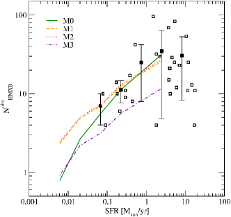
Figure 2: Observed number of HMXBs in nearby, star-forming galaxies, as a function of their SFR. Empty squares represent individual galaxies from the sample of Mineo et al. (2012); filled ones are the mean values in each SFR bin. Model predictions for the mean value of $N_{\rm HMXB}^{\rm obs}$ are plotted for M0 (green, solid line), M1 (orange, dashed line), M2 (red, dotted line) and M3 (violet, dash-dotted line). All models are required to match the data in order to determine the best-fitting $L_{\rm min}$ and $\eta$. M1 and M2 present the same relation. For the sake of clarity, the relation of M2 has been displaced slightly.

In Figs. 2 and 3, we show $N^{\rm obs}_{\rm HMXB}$ and $L^{\rm obs}_{\rm X}$ as a function of SFR for our model predictions and the observations of nearby galaxies of Mineo et al. (2012). All the explored models are required to provide a good fit to the data in order to determine the free parameters. The resulting values for each model are listed in Table 1. The match of the models to the observed data has been done for the range ${\rm SFR}\sim 0.1-2\ M_{\odot}\ {\rm yr}^{-1}$, since there are no galaxies with higher SFRs that fulfil the condition ${\rm sSFR}>10^{-10}\ {\rm yr}^{-1}$ in our simulated catalogues. The dispersions of the model predictions are in the range 0.28–0.44 dex (except for M0, for which it is negligible). These dispersions are in excellent agreement with those measured by Mineo et al. (2012) ($\sim 0.4$ dex), suggesting that the internal chemical inhomogeneity of galaxies might be responsible for the observed dispersion in the $L_{\rm X}$-SFR relation.

When chemistry-dependent XLFs are also considered, we find that choosing the free parameters to match the observed mean number of sources (M2) overestimates the observed mean luminosity of galaxies, while matching the latter (M3) slightly underestimates the former. Unfortunately, the large error bars of the observed data prevent us to prefer one over the other. Hence, we study both of them to explore the consequences of a better fit to either observable. More precise observations will certainly contribute to make a better selection of the free parameters.

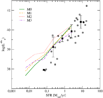
Figure 3: Observed X-ray luminosity of nearby, star-forming galaxies, as a function of their SFR. Empty squares represent individual galaxies; filled ones are the mean values in each SFR bin. Model predictions for the mean value of $L_{\rm X}^{\rm obs}$ are included for M0 (green, solid line), M1 (orange,dashed line), M2 (red, dotted line) and M3 (violet, dash-dotted line). All models are required to match the data in order to select the best-fitting $L_{\rm min}$ and $\eta$ in each case. The dispersions of the model predictions are in the range 0.28–0.44 dex (except for M0, for which it is negligible), and have not been plotted for clarity. The slope of the $L_{\rm X}^{\rm obs}$–SFR relation decreases as the chemical dependence of the model becomes stronger due to the correlation between the SFR and the metallicity of galaxies.

4 HMXBs across cosmic time

To investigate the evolution of the $L_{\rm X}$–SFR relation, we analyse $f_{\rm X}$ as function of redshift (see definition in Section 1). In Fig. 4, we plot $f_{\rm X}$ predicted by our four models as a function of SFR, for different redshifts in the range $z=0.3-3.5$. As expected, for M0 the value of $f_{\rm X}$ is independent of both SFR and redshift since by construction it takes a value of $\sim 0.2$, similar to that observed in the local Universe. This is due to the lack of any metallicity dependences so that all galaxies produce X-ray luminosities proportional to their SFRs, with the same proportionality independently of redshift. The very small dispersion detected for $f_{\rm X}$ originates in the upper metallicity limit for binary systems to be able to produce HMXBs. As explained in the previous section, no HMXB sources are produced for $Z>0.04$. This introduces a small dispersion in the $f_{\rm X}$–SFR relation which gets higher as the metallicity of the interstellar medium from which stars form increases with decreasing redshift.

The effects of the chemical dependence included in M1 can be clearly seen in Fig. 4 which shows how $f_{\rm X}$ increases with increasing redshift, at a given SFR. The correlation between the mean metallicity and SFR of galaxies, in the sense that high-SFR objects tend to be more enriched than low-SFR ones, makes $f_{\rm X}$ to decrease with SFR at given redshift. These effects are consequence of the chemical evolution of the Universe so that galaxies tend to be less enriched at high redshift, producing more HMXBs. The effects discussed above are mild for M1 because they are only driven by the increase in the HMXB production rate with decreasing metallicity. Stronger trends are detected in models M2 and M3 because of the increase in both the HMXB production rate and their X-ray luminosity at low metallicities.

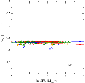
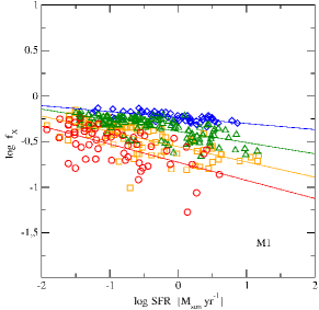
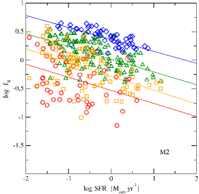
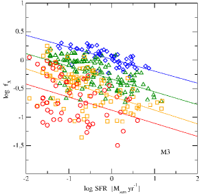
Figure 4: The normalised ratio of the X-ray luminosity of galaxies to their SFR ($f_{\rm X}$) as a function of the latter, for four analysed models. The evolution of this relation is shown for $z=3.5$ (blue diamonds), $z=2$ (green triangles), $z=1$ (orange squares) and $z=0.3$ (red circles). The solid lines represent the best linear fits to the models at each redshift. At fixed redshift, chemistry-dependent models show a decrease of $f_{\rm X}$ with SFR, due to the correlation between the mean metallicity and the SFR of galaxies. The same models present an increase in $f_{\rm X}$ with redshift at fixed SFR, due to the chemical evolution of the Universe. They also show a large dispersion in $f_{\rm X}$, due to the chemical inhomogeneities within each galaxy. All these effects are stronger in M2 and M3 (which include metallicity-dependent of both the rates and the luminosities of the HMXBs) than in M1 (which includes only metallicity-dependent HMXB rates), and are absent in M0 (which includes no metallicity dependence). However, if the data is not analysed as a function of redshift, these parameters determine a relation consistent with a flat $f_{\rm X}$–SFR with a large dispersion.

It is interesting to note that trends shown in Fig. 4 are detected only when galaxies are grouped as a function of redshift. If no redshift information is taken into account, the mean trend is consistent with a flat $f_{\rm X}$–SFR relation, with a large dispersion as the only observable effect of metallicity. We quantify the evolution of the $f_{\rm X}$–SFR relation with cosmic time by performing linear regression fits to the simulated data at different redshifts. Table 2 summarizes the best-fitting parameters, and Fig. 5–7 show the evolution with redshift of the zero point, slope, and dispersion of the fits, respectively.

As can be seen from Fig. 5, between $z\sim 0.3$ and $z\sim 3.5$, the zero point varies by $\sim 0.5\ {\rm dex}$ for M1 and by $\sim 1\ {\rm dex}$ for M2 and M3 (no evolution is seen for M0 as expected). As explained above, this variation is caused by the global chemical enrichment of the galaxies as they evolve. At low redshift, galaxies tend to be more chemically enriched, leading to lower $f_{\rm X}$ values. M2 and M3 show the same zero-point trend with redshift, but the actual values differ by $\sim 0.4\ {\rm dex}$. This is consistent with the construction process as M2 was forced to fit the number of sources in nearby galaxies, hence overestimating the galaxy luminosities, and M3 was forced to fit the X-ray luminosities themselves.

Fig. 6 shows the evolution of the slope of $f_{\rm X}$–SFR relations with cosmic time. For M0, the slope of the $f_{\rm X}$–SFR relation is almost null at all redshifts, as expected. For M1, we detect a variation from $\sim-0.1$ to $\sim-0.2$ in the analysed redshift range. The negative value of the slope arises from the correlation between the mean galaxy metallicity and SFR. Because of this correlation, low-SFR galaxies tend to have preferentially low metallicities, hence chemistry-dependent models produce higher $f_{\rm X}$ values for them. The variation of the slope with redshift is due to the evolution of this correlation. The metallicity difference between low-SFR and high-SFR objects increases with decreasing redshift, as a consequence of their different chemical evolution. The absolute value of the (negative) slope of the $f_{\rm X}$–SFR relation follows this behaviour, which is clearly seen in Fig. 6. For M2 and M3, the value of the slope at any redshift is lower than that of M1, due to the stronger dependence of HMXB properties on metallicity in these models. The lack of evolution of the slope with redshift in M2 and M3 can be understood by comparison with M1, recalling that M2 and M3 also include a strong increase in the luminosity of the most metal-poor stellar populations. For low redshifts there are few such stellar populations, and they are present mainly in low-SFR galaxies. Hence, M2 and M3 produce a small increase (with respect to M1) in the luminosities of these galaxies, making the slope of the $f_{\rm X}$–SFR relation slightly more negative than in M1. For high redshifts, very low metallicity stellar populations are ubiquitous. The fraction of the star formation that proceeds at these metallicities increases as the SFR decreases, due to the SFR-metallicity correlation. The high X-ray luminosities of these stellar populations amplify the effect of the variation of the number of HMXBs with metallicity. Therefore, the slope of the $f_{\rm X}$–SFR relation is much more negative in M2 and M3 than in M1 for these redshifts. As a consequence, in M2 and M3 the slope attains similar values. Intermediate values of $L_{\rm max}(Z_{1})$ between the two tested maximum limits produce relations in between the ones shown in Fig. 6. Hence, if the slope of $f_{\rm X}$–SFR could be measured observationally as a function of redshift, it could provide information not only on the existence of a metallicity-dependence of the X-ray luminosity of the HMXBs but also on the maximum value it could attain.

The dispersion of the $f_{\rm X}$–SFR relation for the simulated HMXBs also change with cosmic times. As it has been discussed above, the dispersion is originated by the chemical inhomogeneity of stellar populations in the simulated galaxies, which is then reflected in the generated HMXB sources in those chemistry-dependent models. As a consequence, for M0 the dispersion is negligible at any redshift (Fig. 7). For M1, the dispersion decreases from $\sim 0.1$ at low redshifts to $\sim 0.04$ at $z\sim 3.5$, because for higher redshifts galaxies are both less chemically enriched and have lower metallicity dispersions. The same trend is seen in M2 and M3 showing an increase from $\sim 0.1$ at $z\sim 3.5$ to $\sim 0.35$ at $z\sim 0.3$. The higher dispersions detected in M2 and M3 compared to those in M1 are due to the fact that the formers also include the dependence on metallicity of the X-ray luminosities of HMXBs as already mentioned.

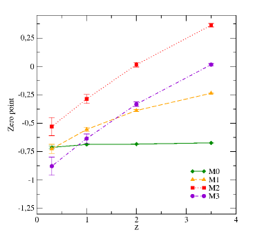
Figure 5: Zero point of the best linear fit to the logarithmic $f_{\rm X}$–SFR relation for each model (M0, green solid line and diamonds; M1, orange dashed line and triangles; M2, red dotted line and squares; M3, violet dot-dashed line and circles), as a function of redshift. The zero point of the fit increases with redshift due to the chemical enrichment of the Universe. This increase is larger in models with a stronger chemical dependence (M2 and M3) and almost null in that with no chemical dependence (M0).

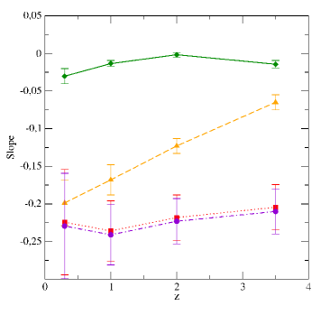
Figure 6: Slope of the best linear fit to the logarithmic $f_{\rm X}$–SFR relation for M0 (green diamonds and solid line), M1 (orange triangles and dashed line), M2 (red squares and dotted line) and M3 (violet circles and dot-dashed line), as a function of redshift. The absolute value of the slope of the fit is larger in models with a stronger chemical dependence (M2 and M3), and almost null in that with no chemical dependence (M0), as expected because of the correlation between the SFR and the mean metallicity of galaxies. M2 and M3 determine the same relation; for the sake of clarity, we shifted slightly M2.

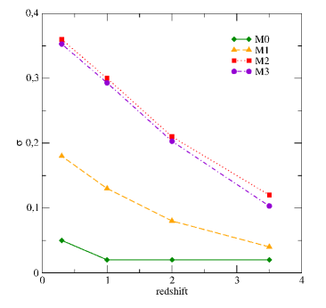
Figure 7: Dispersion of the best linear fit to the logarithmic $f_{\rm X}$–SFR relation for each model (M0, green solid line and diamonds; M1, orange dashed line and triangles; M2, red dotted line and squares; M3, violet dot-dashed line and circles), as a function of redshift. The dispersion of the fit is larger in models with a stronger chemical dependence (M2 and M3) and almost null in that with no chemical dependence (M0), due to the chemical inhomogeneity of the star formation in galaxies. The decrease of the dispersion with redshift arises because at high redshift this inhomogeneity is smaller. M2 and M3 determine the same relation; for sake of clarity, we shifted M2 slightly.

The trend of $f_{\rm X}$ to increase with redshift has been reported to be marginal by Cowie et al. (2012). However, based on a larger set of observations, Basu-Zych et al. (2013) found a clear evolution of $f_{\rm X}$ with redshift, which can be parametrized as $\log f_{\rm X}=(0.93\pm 0.07)\log(1+z)-(0.35\pm 0.03)\log{\rm SFR}-(0.74\pm 0.03)$. We note that this relation includes not only the increase of $f_{\rm X}$ with redshift but also its decrease with SFR. Taken as a function of SFR, the slope and zero point of this parametrization, and the variation of the latter with redshift, are in reasonable agreement with the corresponding predictions of our chemistry-dependent models M1 and M3.

To compare our models with observations of Basu-Zych et al. (2013) in more detail, we use those galaxies with SFR in the range $5-15M_{\odot}\ {\rm yr}^{-1}$. This range was chosen because both models and observations are well represented within it. As can be seen from Fig. 8, only chemistry-dependent models can describe the trend seen in the observations. Model M0 predicts $f_{\rm X}$ values far lower than those observed while M2 is at odds with the upper limits of Basu-Zych et al. (2013). Only M1 and M3 seem to be consistent with the data. This is confirmed by a Bayesian analysis; the posterior probabilities of the models given the data (including upper limits) are non-negligible only for models M1 and M3. M2 shows an excess of X-ray luminosity as expected because of the higher number of sources predicted by this model (see Section 3). These results suggest that the metallicity dependence is needed to explain the data, although more observations and larger simulated volumes are clearly required to improve this comparison.

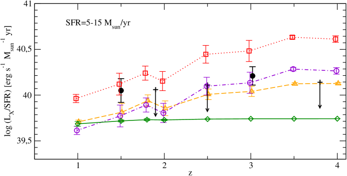
Figure 8: Evolution of the ratio of the mean X-ray luminosity of galaxies to their SFR with redshift, for galaxies with ${\rm SFR}\in[5,15]M_{\odot}\ {\rm yr}^{-1}$. The prediction of our models (M0, green solid line and diamonds; M1, orange dashed line and triangles; M2, red dotted line and squares; M3, violet dot-dashed line and circles) are shown against observed data (black circles and arrows) of Basu-Zych et al. (2013). It is clear from the plot, and confirmed by Bayesian analysis, that only chemistry-dependent models reproduce the trend seen in the observations.

Table 2: Parameters of the best linear regression $\log f_{\rm X}=A\log{\rm SFR}[M_{\odot}\ {\rm yr}^{-1}]+B$ for models M0–M3 at redshifts $z=0.3-3.5$.

Model	$z$	$A$	$B$	$\sigma$
M0	0.3	$-0.03\pm 0.01$	$-0.71\pm 0.01$	0.05
M0	1.0	$-0.010\pm 0.004$	$-0.687\pm 0.003$	0.02
M0	2.0	$\phantom{-}0.002\pm 0.003$	$-0.677\pm 0.003$	0.02
M0	3.5	$\phantom{-}0.014\pm 0.005$	$-0.673\pm 0.003$	0.02
M1	0.3	$-0.19\pm 0.03$	$-0.73\pm 0.05$	0.18
M1	1.0	$-0.17\pm 0.02$	$-0.56\pm 0.02$	0.13
M1	2.0	$-0.12\pm 0.01$	$-0.388\pm 0.009$	0.08
M1	3.5	$-0.065\pm 0.009$	$-0.236\pm 0.005$	0.04
M2	0.3	$-0.22\pm 0.07$	$-0.53\pm 0.08$	0.35
M2	1.0	$-0.24\pm 0.04$	$-0.28\pm 0.04$	0.29
M2	2.0	$-0.22\pm 0.03$	$-0.00\pm 0.02$	0.20
M2	3.5	$-0.21\pm 0.03$	$\phantom{-}0.40\pm 0.01$	0.11
M3	0.3	$-0.23\pm 0.07$	$-0.88\pm 0.08$	0.35
M3	1.0	$-0.24\pm 0.04$	$-0.63\pm 0.04$	0.29
M3	2.0	$-0.22\pm 0.03$	$-0.33\pm 0.02$	0.20
M3	3.5	$-0.21\pm 0.03$	$-0.02\pm 0.01$	0.20

5 Discussion and Summary

Motivated by recent studies which suggest that both the number of HMXBs and their X-ray luminosity might be higher in low-metallicity stellar systems (Belczynski et al. 2004b; Dray 2006; Linden et al. 2010; Mirabel et al. 2011), we explored the consequences of these hypotheses for the X-ray emission of star-forming galaxies, and its cosmological evolution. For this purpose, we develope a model to generate HMXBs which is applied to galaxy catalogues constructed from hydrodynamical cosmological simulations. These simulations include a self-consistent treatment of the chemical evolution of baryons, and consequently, they provide the ages and metallicities of the stellar populations as galaxies form and evolve. As a function of time, each galaxy is described as mixture of stellar populations with different metallicities and ages. By using our HMXBs we can follow the formation of these events at different stages of evolution of the Universe and confront them with observations to constrain the free parameters of the models.

We first confront our models with observations in nearby galaxies (Mineo et al. 2012) to estimate the free parameters. Then, we apply them to investigate the variations of the HMXB properties across cosmic time. We explore a non-metallicity dependent model and three other ones with metallicity dependences in the production rate and X-ray luminosities.

We detect a significant dispersion in the $L_{\rm X}$–SFR relation for our simulated local-Universe galaxies in the range $\sim 0.28-0.44$ dex, comparable to the $\sim 0.4$ dex reported by Mineo et al. (2012). Hence, our results suggest that the internal metallicity dispersion of galaxies combined with the metallicity dependence of the X-ray sources might provide the physical origin for the observed dispersion in the $L_{\rm X}$–SFR relation.

We explored the cosmological evolution of the ratio between the X-ray luminosity of galaxies and their SFR, parametrized by the factor $f_{\rm X}$. The confrontation of our models with the observations of Basu-Zych et al. (2013) favours models with metallicity dependence, and rejects those in which metallicity plays a negligible role. However, the nature of this dependence cannot be determined by using these observations. Both a dependence of the HMXB production rate on metallicity (M1), and this one plus a metallicity-dependent HMXB luminosity (M3) fit the data as well. More precise measurements of $f_{\rm X}$–SFR relation as a function of redshift would help us to establish its nature.

In fact, three main trends are detected in our chemistry-dependent models, which might be used by observers to test the existence of a chemical dependence in the rate of production or in the luminosities of HMXBs:

• At given redshift, a decrease of $f_{\rm X}$ with the SFR of galaxies is detected due to the correlation between the mean metallicity of galaxies and their SFR. This correlation makes low-SFR galaxies have lower metallicity and hence, higher $f_{\rm X}$ that high-SFR ones. Our models predict a weak decrease if a metallicity dependence for the production rates is adopted ($\sim 0.15$ dex) and a stronger one if this dependence is extended to the X-ray luminosities ($\sim 0.25$ dex).

• For galaxies with similar SFRs, $f_{\rm X}$ should decrease with decreasing redshift because galaxies evolve to higher mean metallicities for decreasing redshift. Again, the level of decrease is predicted to be directly related to the metallicity dependence: the higher it is, the larger the change with redshift. In our models, $f_{\rm X}$ increases by $\sim 0.5\ {\rm dex}$ between $z\sim 0$ and $z\sim 3.5$ for a metallicity-dependent HMXB rate, and by $\sim 1\ {\rm dex}$ in the same redshift range if metallicity affects both the rates and the X-ray luminosities of HMXBs.

• The $f_{\rm X}$–SFR relation shows a dispersion which reflects the combined effects of the chemical evolution of the stellar populations and the metallicity dependences of the X-ray sources. This dispersion should decrease with increasing redshift since high-redshift galaxies tend to have stellar populations with more homogeneous metallicity distributions. Our findings suggest that the variation of the dispersion with redshift store information on the nature of the metallicity dependence.

None of these three effects is predicted in a scenario with a negligible metallicity dependence of the properties of HMXBs. Hence the observational measurement of any of them would make a strong case for this dependence.

Our results suggest that the evolution of the $f_{\rm X}$–SFR relation should be observed up to high redshift and low SFRs in order to assess the chemical dependence of the properties of HMXB populations. The study of the properties of HMXB populations through cosmic times can unveil their potential contribution to energy feedback, which is expected to play a critical role in the thermal and ionization history of the Universe (e.g. Mirabel et al. 2011; Justham & Schawinski 2012; Fragos et al. 2013b; Jeon et al. 2013). In a future work we explore the effects that energy feedback from HMBXs might have on the regulation of the star formation in early Universe.

References

- Artale et al. (2011) Artale, M. C., Pellizza, L. J., & Tissera, P. B. 2011, MNRAS, 415, 3417
- Basu-Zych et al. (2013) Basu-Zych, A. R., Lehmer, B. D., Hornschemeier, A. E., et al. 2013, ApJ, 762, 45
- Belczynski et al. (2010a) Belczynski, K., Bulik, T., Fryer, C. L., et al. 2010a, ApJ, 714, 1217
- Belczynski et al. (2010b) Belczynski, K., Dominik, M., Bulik, T., et al. 2010b, ApJ, 715, L138
- Belczynski et al. (2004a) Belczynski, K., Kalogera, V., Zezas, A., & Fabbiano, G. 2004a, ApJ, 601, L147
- Belczynski et al. (2004b) Belczynski, K., Sadowski, A., & Rasio, F. A. 2004b, ApJ, 611, 1068
- Belczynski et al. (2008) Belczynski, K., Taam, R. E., Rantsiou, E., & van der Sluys, M. 2008, ApJ, 682, 474
- Chisari et al. (2010) Chisari, N. E., Tissera, P. B., & Pellizza, L. J. 2010, MNRAS, 408, 647
- Cowie et al. (2012) Cowie, L. L., Barger, A. J., & Hasinger, G. 2012, ApJ, 748, 50
- De Rossi et al. (2013) De Rossi, M. E., Avila-Reese, V., Tissera, P. B., González-Samaniego, A., & Pedrosa, S. E. 2013, MNRAS, 435, 2736
- de Rossi et al. (2010) de Rossi, M. E., Tissera, P. B., & Pedrosa, S. E. 2010, A&A, 519, A89
- De Rossi et al. (2012) De Rossi, M. E., Tissera, P. B., & Pedrosa, S. E. 2012, A&A, 546, A52
- Dijkstra et al. (2012) Dijkstra, M., Gilfanov, M., Loeb, A., & Sunyaev, R. 2012, MNRAS, 421, 213
- Dray (2006) Dray, L. M. 2006, MNRAS, 370, 2079
- Fabbiano (2006) Fabbiano, G. 2006, ARA&A, 44, 323
- Feng & Soria (2011) Feng, H. & Soria, R. 2011, New A Rev., 55, 166
- Fragos et al. (2013a) Fragos, T., Lehmer, B., Tremmel, M., et al. 2013a, ApJ, 764, 41
- Fragos et al. (2013b) Fragos, T., Lehmer, B. D., Naoz, S., Zezas, A., & Basu-Zych, A. 2013b, ApJ, 776, L31
- Georgy et al. (2009) Georgy, C., Meynet, G., Walder, R., Folini, D., & Maeder, A. 2009, A&A, 502, 611
- Grimm et al. (2003) Grimm, H.-J., Gilfanov, M., & Sunyaev, R. 2003, MNRAS, 339, 793
- Jeon et al. (2013) Jeon, M., Pawlik, A. H., Bromm, V., & Milosavljevic, M. 2013, ArXiv e-prints
- Justham & Schawinski (2012) Justham, S. & Schawinski, K. 2012, MNRAS, 423, 1641
- Kaaret et al. (2011) Kaaret, P., Schmitt, J., & Gorski, M. 2011, ApJ, 741, 10
- Linden et al. (2010) Linden, T., Kalogera, V., Sepinsky, J. F., et al. 2010, ApJ, 725, 1984
- Maiolino et al. (2008) Maiolino, R., Nagao, T., Grazian, A., et al. 2008, A&A, 488, 463
- Mineo et al. (2012) Mineo, S., Gilfanov, M., & Sunyaev, R. 2012, MNRAS, 419, 2095
- Mirabel et al. (2011) Mirabel, I. F., Dijkstra, M., Laurent, P., Loeb, A., & Pritchard, J. R. 2011, A&A, 528, A149
- Mosconi et al. (2001) Mosconi, M. B., Tissera, P. B., Lambas, D. G., & Cora, S. A. 2001, MNRAS, 325, 34
- Nuza et al. (2007) Nuza, S. E., Tissera, P. B., Pellizza, L. J., et al. 2007, MNRAS, 375, 665
- Pedrosa et al. (2014) Pedrosa, S. E., Tissera, P. B., & De Rossi, M. E. 2014, ArXiv e-prints
- Pellizza et al. (2012) Pellizza, L. J., Artale, M. C., & Tissera, P. B. 2012, in Gamma-Ray Bursts 2012 Conference (GRB 2012)
- Power et al. (2013) Power, C., James, G., Combet, C., & Wynn, G. 2013, ApJ, 764, 76
- Power et al. (2009) Power, C., Wynn, G. A., Combet, C., & Wilkinson, M. I. 2009, MNRAS, 395, 1146
- Salpeter (1955) Salpeter, E. E. 1955, ApJ, 121, 161
- Scannapieco et al. (2005) Scannapieco, C., Tissera, P. B., White, S. D. M., & Springel, V. 2005, MNRAS, 364, 552
- Scannapieco et al. (2006) Scannapieco, C., Tissera, P. B., White, S. D. M., & Springel, V. 2006, MNRAS, 371, 1125
- Shtykovskiy & Gilfanov (2007) Shtykovskiy, P. E. & Gilfanov, M. R. 2007, Astronomy Letters, 33, 437
- Springel (2005) Springel, V. 2005, MNRAS, 364, 1105
- Springel et al. (2001) Springel, V., White, S. D. M., Tormen, G., & Kauffmann, G. 2001, MNRAS, 328, 726
- Thielemann et al. (1993) Thielemann, F. K., Nomoto, K., & Hashimoto, M. 1993, Origin and Evolution of Elements, 1st edn., ed. N. Prantzos, E. Vangoni-Flam, & N. Cass (Cambridge: Cambridge Univ. Press), p. 299
- Tremonti et al. (2004) Tremonti, C. A., Heckman, T. M., Kauffmann, G., et al. 2004, ApJ, 613, 898
- Woosley & Weaver (1995) Woosley, S. E. & Weaver, T. A. 1995, ApJS, 101, 181
- Zuo & Li (2011) Zuo, Z.-Y. & Li, X.-D. 2011, ApJ, 733, 5