Universal features of exit probability in opinion dynamics models with domain size dependent dynamics
Abstract
We study the exit probability for several binary opinion dynamics models in one dimension in which the opinion state (represented by ) of an agent is determined by dynamical rules dependent on the size of its neighbouring domains. In all these models, we find the exit probability behaves like a step function in the thermodynamic limit. In a finite system of size , the exit probability as a function of the initial fraction of one type of opinion is given by with a universal value of . The form of the scaling function is also universal: , where is found to be dependent on the particular dynamics. The variation of against the parameters of the models is studied. is non-zero only when the dynamical rule distinguishes between states; comparison with theoretical estimates in this case shows very good agreement.
pacs:
89.75.Da, 89.65.-s, 64.60.De, 75.78.Fg1 Introduction
Identifying universality in physical phenomena occurring in different systems has become an important topic of research in the last few decades. Universality usually indicates that there are some fundamental common underlying features in the systems under consideration. It also signifies that there are only a few parameters occurring in the systems those are relevant. Existence of universality justifies the study of models which include only these parameters while real systems are far more complicated. Universality has been observed in critical phenomena; for example there is a unique value of the order parameter exponent in liquid-gas phase transition [1]. Universal features may also appear away from criticality as for example the universal scaling behaviour obtained for characteristic features of many complex networks [2]. In dynamical phenomena, universal classes have been observed close to and away from criticality. Models belonging to the same static universality class may belong to a different universality class as far as dynamics is concerned [3]. Non-equilibrium dynamics also reveal dynamical universal classes, for example, many systems have been shown to belong to the directed percolation universality class [4, 5].
Exit probability (EP) is one important feature of dynamical models with two absorbing states. Examples include binary opinion dynamics models and Ising spin models. Exit probability denotes the probability that the system ends up with all opinion/spins in a certain state when initially fraction had been in that state. Recently, a lot of effort has been put to identify universal features of exit probability in opinion dynamics models (as well as generalised Ising-Glauber models) in one dimension. In the voter model (which is equivalent to the Ising-Glauber dynamics in one-dimension) is simply equal to while is a non-linear continuous function of in nonlinear voter model, Sznajd model and long ranged Ising Glauber model [6, 7, 8, 9] in one dimension. In all these cases apparently shows no dependence on finite sizes for larger system sizes [6]. The exit probability was also calculated and generalised for nonlinear q-voter model in one-dimension [10, 11, 12]. In higher dimensions or on networks, the exit probability in the thermodynamic limit may exhibit a step function behaviour, interpreted as a phase transition in some earlier works [13, 14, 15, 16, 17]. Strong finite size effects are observed here. The possibility of problems arising while calculating the exit probability, due to the sole use of local update rules in dynamical systems, was addressed previously by Galam et al [18].
In a recent study of a binary opinion dynamics model [19], the behaviour of the exit probability was found to be quite different from the well studied models mentioned in the paragraph above; it exhibited a step function like behaviour in the thermodynamic limit even in one dimension. It also showed the existence of an exponent with a value independent of the model parameter. In the model considered in [19], the state (spin or opinion) of an agent was updated according to a rule dependent on the size of his/her two neighbouring domains.
In this paper, we investigate whether the step function behaviour of in the thermodynamic limit is a universal feature of models with dynamical rules which involve the sizes of neighbouring domains in one dimension. Careful study of a number of models indicates that indeed such a universal feature exists. Furthermore, universal scaling function and an exponent with model independent universal value are obtained. The non-universal quantities associated with the scaling function also show very interesting behaviour as a function of the model parameters.
In section II, the models are introduced and details of the simulation provided briefly. Results are presented in section III and discussions and summary in the last section.
2 The Models
We have considered a number of models which mimic opinion formation in a society where the opinions have values . These states can be equivalently regarded as the states of Ising spins and the models may be interpreted as interacting spin models as well. Since it is convenient to talk in terms of spins we will use the term spin instead of opinion henceforth. It also becomes more meaningful as the models behave as familiar spin models in certain limits.
In all these models considered in one dimension, in the spin picture, the spins located on the domain boundaries are liable to flip, as in the case of zero temperature Ising model with Glauber dynamics. The spins which can undergo change have therefore two neigbouring domains of opposite spin states. In general, in the models considered in this work, the state of the spin at the domain boundary is determined by the state of the neighbouring domains and their sizes.
2.0.1 BS model
In the first model introduced in this class by Biswas and Sen [20], the BS model hereafter, the state of the spin simply follows that of the larger neighbouring domain. Hence if and are the neighbouring domain sizes (with up and down spins respectively), the spin will be up if and down otherwise. In case , the state is chosen to be with equal probability. A spin sandwiched between domains of opposite sign is always flipped. The BS model, where the final configuration is all up or all down states, is different from the Ising model having different dynamical exponents with respect to domain growth and persistence [20].
2.0.2 BS model with cutoff
In the BS model one can introduce a cutoff [21] on the size of the domain while calculating and . The cutoff is taken as where is the system size and a parameter ranging from zero to 1. Now, with the introduction of this cut off parameter , the definition of and are modified: and similarly while the same dynamical rule explained earlier applies. When is infinitesimal, the results are identical to those of the nearest neighbour Ising model. For finite , there is a crossover behaviour in time: initially there is a BS-like behaviour after which very few domain walls survive which perform almost noninteracting motion for a long time before annihilating each other. is of course equivalent to the BS model. Instead of a fixed value of the cutoff a random cutoff can also be considered.
2.0.3 The model
We have also studied a model where the dynamics depends on the size of the neighbouring domains stochastically with a noise like parameter [22]. In this so called model, the probability of a boundary spin to be up is taken as
| (1) |
and it is down with probability
| (2) |
The normalised probabilities are therefore and , where . is equivalent to the Ising model and any finite value of drives the system to the BS dynamical class.
2.0.4 The model
The BS model was shown to be equivalent to a reaction diffusion model in one dimension where random walkers tend to walk towards their nearer neighbours and annihilate on meeting [23]. This reaction diffusion model can be generalised by assigning a probability to move towards the nearer neighbour. corresponds to the BS model and , the model with unbiased walkers which mimics the coarsening dynamics in the Ising model. We call this model the model. In the equivalent spin model, the larger neighbouring domain will dictate the sign of the spin on the boundary with probability .
2.0.5 The model
Another stochastic model involving two parameters has been conceived [20]. Here a quenched disorder is introduced in the BS model through a parameter representing the probability that people are completely rigid and never change their opinion throughout the time evolution. The second parameter relaxes the rigidity criterion in an annealed manner. It was found that although with and , no consensus state is reached, any nonzero value of enables the system to reach the all up/down states [20].
2.0.6 The weighted influence (WI) model
In all the models described above, the up and down states are taken to be indistinguishable. A model in which the up and down domains have different weight factors has been considered recently [19] and in fact the exit probability was also evaluated as mentioned in the introduction. We apply the analysis used in this work to the results of [19] to reveal certain interesting features related to the exit probability. This model was termed as the weighted influence (WI) model, where an individual takes up opinion with probability
| (3) |
is the relative influencing ability of the two groups and can vary from zero to . Probability to take opinion value is
All the models discussed above have one common feature in their dynamical rule. For all these models the state of the randomly selected spin depends on the size of the neighbouring domains somehow. In spite of this similarity the intrinsic dynamical rule of the models are different. The first one is the BS model which has no disorder, no stochasticity in the dynamics and the state of the selected spin becomes just the same as that of the larger neighbouring domain. Also in the BS model with cutoff there is no intrinsic stochasticity and disorder but its late time dynamical behaviour is completely different which is Ising like. In the model, thermal noise like disorder is introduced. Here the dynamics is stochastic but for any non-zero the system belongs to the dynamical class of BS model. In the model disorder is introduced through and . For , this model has the same dynamical behaviour as the BS model. In the model, with , dynamical behaviour is same as BS model whereas for the dynamics is Ising like and for a different behaviour has been observed previously. On the other hand the WI model, which incorporates stochasticity, is not equivalent to the BS model in any limit. It belongs to a different universality class as far as persistence behaviour is concerned.
System sizes ranging from to were considered depending on the model; e.g., since the BS model does not involve any parameter, one could probe much larger sizes 111In fact to get reliable results for the dynamic exponents in the BS model one needs to simulate systems with size at least [20, 21, 22, 23].. All the simulations are done for at least configurations for each system size. Random sequential updating is used in all the simulations.
3 Results
3.1 Symmetric models: Exit probability
We first discuss the results for the behaviour of the EP for the models with symmetry where up/down states have the same status. These results show the existence of an exponent with a model independent universal value.
3.1.1 BS model
For the BS model we have studied the exit probability for system sizes ranging from to . The plot of against initial fraction of up spins shows that it is nonlinear having strong system size dependence and that the different curves intersect at a single point (shown in the inset of Fig. 1). The curves become steeper as the system size is increased. The exit probability thus shows a step function behaviour in the thermodynamic limit.
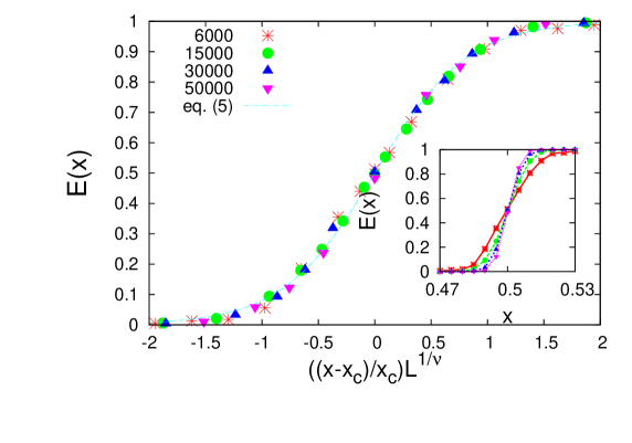
Finite size scaling analysis can be made using the scaling form
| (4) |
where for and equal to for , so that the data for different system sizes collapse when is plotted against . The data collapse takes place with (Fig. 1). The value of has been estimated as follows: ideally at the exit probability is size independent. Numerically it is difficult to obtain exact intersection for all the system sizes. Above , data for larger values of system size lie above in the vs plane, and below the opposite happens, so by observing the range of x for which this happens, the error bars are estimated. To obtain , one uses the value of obtained as above and the range of values for which the collapse appears to be good is taken to estimate the error bars. However, a good scaling collapse can only be obtained for sufficiently large values of , typically .
3.1.2 BS model with cutoff
Introducing a cutoff in the BS model, we calculate using cutoff factor for different system sizes ranging from to . As long as , the time to reach equilibrium . So here we have to restrict system size at while for other models we use much larger system sizes.
3.1.3 The model
In the model we have studied the exit probability with noise parameter for system sizes ranging from to . For the plot of against gives a straight line (Fig. 3) which is expected as it is identical to the nearest neighbour Ising model. In this case the result is independent of finite system sizes also.

3.1.4 The model
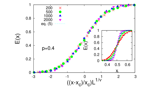
In the model we have studied the exit probability with rigidity parameter for using different system sizes ranging from to . For this model also, EP shows a nonlinear behaviour with strong system size dependence (Fig. 4). Here also shows scaling behaviour given by eq. (4) with scaling exponent independent of and . Also for all values of and .
3.1.5 The model
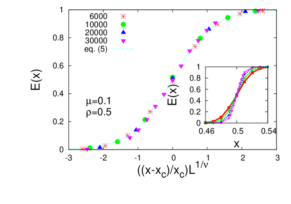
For the model the system reaches the consensus state (all up/down) only for . In fact when , the final state is completely disordered.
is simply equal to for which is expected as it is identical to the nearest neighbour Ising model. When , EP shows nonlinear behaviour with strong system size dependence (Fig. 5 shown for ) for any value of .
The system sizes here vary from to . Data collapse similar to the previously discussed models is also obtained here (Fig. 5) with and .
3.2 Analysis of the scaling function for symmetric models
We find that in all the above cases, the EP becomes a step function at in the thermodynamic limit and the scaling form given by eq. (4) is obeyed with the value of being model independent. The scaling function is found to fit very well with the general form
| (5) |
where . We conjecture the above form from the following considerations: first, the shape of the curve suggests a form (note that the argument varies from to ). Secondly, in the thermodynamic limit (), for and for such that one needs to add a factor of unity and also a division by 2 in . This form also leads to the result that and in the symmetric models, shown later in this subsection.
We obtain the values of and find that is the factor which is different in each case (Figs 6, 7). For the BS model we found by fitting the collapsed plot of the model (fig 1) in equation 5.
When the model involves a parameter, shows variation with the parameter value.
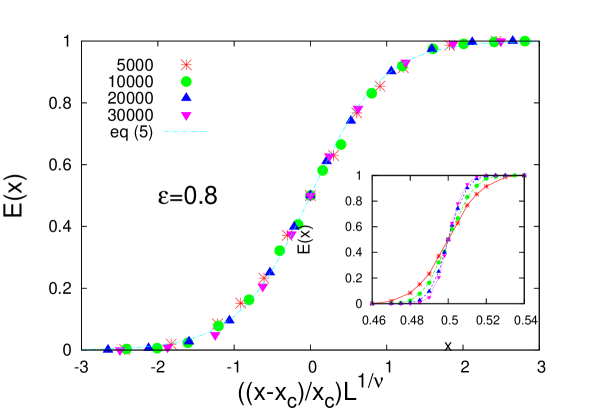
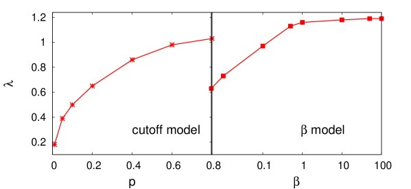
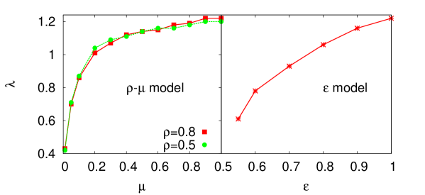
In the cutoff model, model and the models, there are limiting values for which the models coincide with the Ising model and is undefined. On the other hand, for the model, for , is undefined as the dynamics do not lead to the all up/down state. As one increases the parameter values beyond that corresponding to the Ising limit in the first three models mentioned above and in the model, one finds that increases. Each of these four models becomes equivalent to the BS model in the other extreme limiting values of the parameters used. Equivalence to the BS model is achieved in the cutoff model at ; in the model, for ; in the model for and in the model for though the BS model behaviour may be present for even lesser values of the parameters as far as dynamical exponents are concerned. We find that varies monotonically and reaches a maximum value in the BS limit in general: in the cutoff model, model and model for other values of the parameter while in the model, appears to assume the BS model value beyond a finite value .
In the cutoff model, a significant change in the timescale occurs as [21] and the behaviour of against close to unity is no longer very smooth. For this reason, we show the results up to . The values of for the model shows a rather intriguing behaviour: it has an increasing behaviour for and beyond , increases very slowly and is almost a constant while approaching the BS value. However, there was no perceivable difference observed at when other dynamical properties of this model were studied [22]. In the model, though depends on , we found it to be independent of within error bars. It is due to the fact that is an irrelevant parameter, while is a relevant parameter as shown in [20].
In general, one can now use eq. (5) to write down EP for the symmetric models as
| (6) |
In all these models, = 1/2 which can be established from symmetry arguments. In the BS model, one has no parameter and has a unique value. Using the relation
| (7) |
and putting the expression for from eq.(6), one can easily show that has to be equal to and . In the other models we find that has a dependence on the parameter value and in principle one can assume to be a function of the parameter also, but the observed scaling form and the fact that eq. (7) has to be true for all and leads to the result that always.
3.3 Analysis for the asymmetric WI model
In the WI model, it had already been noted that the value has to be used to obtain a data collapse. The EP here is found to be of the form
| (8) |
where ; and all vary with .
In this model, as the up and down spins have different status, it has to be noted that the probability that the final state is all down starting with down spins will not be the same as for up spins. Rather, to consider the negative spin case, one has to replace by such that
| (9) |
We use the short-hand notation for , for and for . For , we use primed variables, e.g. for . Putting the expression of in eq. (9), we get
On simplification one gets
| (10) |
Since and cannot have any dependence then,
| (11) |
For the right hand side of (10) to be zero for any value of ,
| (12) |
and,
| (13) |
Eliminating and from equations (12) and (13) we have,
| (14) |
which is consistent with the fact that replaced by indicates replaced by which is the basis of eq. (9). We have checked that equations (12) and (13) show excellent matching with numerical data. For example for , we obtain and and ( as ) the corresponding values for are and . Inserting these values we find nearly perfect agreement of both sides of equations (12) and (13). However, this can be checked for any other values of by extrapolating the curve shown in the bottom inset of Fig. 8 and indeed one can get good agreement.
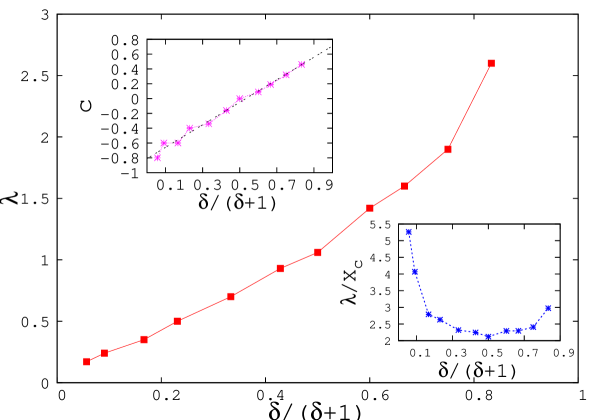
Since the data for has a lot of fluctuations for small values of (see inset of Fig. 8 ), a direct check of eq. (11) is difficult. However, from the figure appears to vary linearly with and one can assume the form
| (15) |
In case eq. (11) is correct, one must have . We tried the above form and the fit appears to be quite accurate with and which shows that is very close to within error bar. This shows that indeed the scaling form we assumed is consistent with the theory.
In the case of WI model, where is different for different , slope of is determined by which shows a minimum at and increases otherwise (Fig. 8, bottom inset). Thus any asymmetry makes the EP steeper which is also expected as the asymmetry makes the system biased towards one of the absorbing states.
4 Summary and discussion
We have studied a number of opinion dynamics models in one dimension with different evolutionary rules for the state of the opinions/spins. A common feature is that the update rules involve the size of the domains neighbouring a spin. This immediately gives rise to a different behaviour of the exit probability compared to that in the well-studied models in one dimension. It shows finite size dependence and a step function like behaviour in the thermodynamic limit. The step function occurs at for models in which up and down states carry equal weight.
A scaling function with a universal form is found to exist with a universal value of the exponent occurring in it. Though the scaling function involves a term is a conjecture, however, we have shown that such a conjecture leads to consistent and meaningful results. Two non-universal parameters and appear in the scaling function. is zero for models which have up/down symmetry. has strong model dependence and it shows interesting variation with the model parameters.
The scaling argument for the finite size scaling is , which indicates that the width of the region where is not equal to unity or zero decreases as . When the rule is simply a majority rule, i.e., the larger neighbouring domain dictates the updated state of the spin (BS model), the value of is obtained as . For the symmetric models which involve a parameter, is smaller than the BS value while is still equal to 0.5. This signifies that is larger for all these models compared to the BS model. In the WI model where up/down spins are distinguished, is larger than the BS value as deviates from unity showing that in this case is smaller than the BS value. Asymmetry thus plays a strong role in determining the width .
In the analysis of the WI model, one can further derive equations connecting the values of , and at and using eq. (8), which shows very good agreement with numerical data.
We thus arrive at the conclusion that there exists a class of models in one dimension that shows a behaviour different from familiar short range spin models in term of EP. Studying different models all of which use a dynamical rule involving the size of the neighbouring domains, a universal scaling behaviour accompanied by an exponent with universal value is obtained. The coarsening behaviour of the models considered here are not identical, e.g., the cutoff model has a Ising-like late time dynamics (domain growth exponent [21]) while the other models show BS like behaviour (). Hence the step function behaviour of EP is clearly due to the domain size dependent dynamics as it is known that for the Ising model EP is just a linear function independent of system size. Asymmetry plays an important role but the value of is not affected.
5 Acknowledgement
We acknowledge D. Dhar for a critical reading of an earlier version of the manuscript. PR acknowledges financial support from UGC. PS acknowledges financial support from CSIR project. SB thanks the Department of Theoretical Physics, TIFR, for the use of its computational resources.
References
References
- [1] See e.g. S. K. Ma, Modern Theory of Critical Phenomena, Perseus Books, Massachusetts (1976).
- [2] See e.g. P. Sen and B. K. Chakrabarti, Sociophysics: An Introduction, Oxford University Press, Oxford (2013).
- [3] P. C. Hohenberg and B. I. Halperin, Rev. Mod. Phys. 49, 435 (1977).
- [4] G. Odor, Rev. Mod. Phys. 76, 663 (2004).
- [5] H. Hinrichsen, Adv. Phys. 49, 815 (2000).
- [6] C. Castellano and R. Pastor-Satorras, Phys. Rev. E 83, 016113 (2011).
- [7] F. Slanina, K. Sznajd-Weron and P. Przybyla, Europhys.Lett. 82, 18006 (2008).
- [8] R. Lambiotte and S. Redner, Europhys. Lett. 82, 18007 (2008).
- [9] P. Roy, S. Biswas and P. Sen, Phys. Rev. E 89, 030103(R) (2014).
- [10] P. Przybyla, K. Sznajd-Weron, and M. Tabiszewski, Phys. Rev. E 84, 031117 (2011).
- [11] A. M. Timpanaro and C. P. C. Prado, Phys. Rev. E 89, 052808, (2014).
- [12] A. M. Timpanaro and S. Galam, arXiv:1408.2734 (2014).
- [13] D. Stauffer, A. O. Sousa and S. M. de Oliveira, Int. J. Mod. Phys. C. 11, 1239 (2000).
- [14] N. Crokidakis and P. M. C. de Oliveira, J. Stat. Mech. (2011) P11004 and the references therein.
- [15] A.O. Sousa , T. Yu-Song and M. Ausloos, European Physical Journal B 66, 115 (2008).
- [16] N. Crokidakis and F. L. Forgerini, Brazilian Journal of Physics 42, 125 (2012).
- [17] A. A. Moreira, J. S. Andrade JR., D. Stauffer, Int. J. Mod. Phys. C 12, 39 (2001).
- [18] S. Galam and A. C. R. Martins, EPL, 95, 48005 (2011).
- [19] S. Biswas, S. Sinha and P. Sen, Phys. Rev. E 88, 022152 (2013).
- [20] S. Biswas and P. Sen, Phys. Rev. E 80, 027101 (2009).
- [21] S. Biswas and P. Sen, J. Phys. A: Math. Theor. 44, 145003 (2011).
- [22] P. Sen, Phys. Rev. E 81, 032103 (2010).
- [23] S. Biswas, P. Sen and P. Ray, Journal of Physics: Conf. Series 297, 012003 (2011).