Ángel Paredes¹, David Novoa², Daniele Tommasini¹ and Héctor Mas¹

¹ Departamento de Física Aplicada, Universidade de Vigo, As Lagoas s/n, Ourense, ES-32004 Spain;
² Max Planck Institute for the Science of Light, Günther-Scharowsky Str. 1, 91058 Erlangen, Germany.

Corresponding author: angel.paredes@uvigo.es

Abstract

One of the latest proposed applications of ultra-intense laser pulses is their possible use to gauge extreme high vacuum by measuring the photon radiation resulting from nonlinear Thomson scattering within a vacuum tube. Here, we provide a complete analysis of the process, computing the expected rates and spectra both for linear and circular polarizations of the laser pulses, taking into account the effect of the time envelope in a slowly-varying envelope approximation. We also design a realistic experimental configuration allowing for the implementation of the idea and compute the corresponding geometric efficiencies. Finally, we develop an optimization procedure for this Photonic Gauge of Extreme High Vacuum at high repetition rate Petawatt and multi-Petawatt laser facilities, such as VEGA, JuSPARC and ELI.

Introduction

Since the invention of chirped pulse amplification [1], the achievable peak intensity of laser light has increased by more than eight orders of magnitude. The current record intensity, achieved at HERCULES few years ago [2], is $2\times 10^{22}$ W/cm², and it may be improved by an order of magnitude by focusing Petawatt (PW) laser pulses close to the diffraction limit. Such enormous intensities are obtained by squeezing the laser pulses both in space and in time, packing a huge number of photons ($\sim 10^{20}$ for a PW laser of duration 30 fs and wavelength $\lambda_{0}=800$nm) in a volume of the order of a few $\mu$m³.

These new sources of radiation have very relevant implications in many fields, such as charged particle acceleration, fast ignition of fusion targets, laboratory simulation of astrophysical conditions and experimental probing of extreme physical regimes [3, 4]. In addition, they have been proposed as new tools to test the quantum polarization properties of the vacuum [5] and search for new physics, such as axion-like or mini charged particles [6].

Recently, it has been suggested [7] that they can also be used to gauge Extreme High-Vacuum (XHV) [8, 9, 10], corresponding to pressures $p<10^{-10}$ Pa. Having a set-up without the electric field of usual ionization gauges may be useful to circumvent their limitations—see also [11, 12] for alternative approaches to XHV gauging. This application of ultra intense lasers to vacuum science is of topical interest since the number and availability of such facilities is expected to increase at a very significant rate in the near future. Moreover, many of the experiments that have been proposed to search vacuum polarization effects and new physics at such facilities, as cited above [5, 6], require the generation and calibration of XHV to control the background noise stemming from the interaction of the laser pulse with the classical vacuum and compute the final sensitivities for the signal. The fact that this can be done using the ultra intense laser itself is a most welcome result.

The idea behind this proposal is fairly simple: photons from the laser pulse are scattered by electrons in the vacuum chamber. The number of scattered photons is directly proportional to the electron density and therefore to the pressure. Background noise can in principle be kept below the signal by appropriately synchronizing the measurements to the passage of the pulse through the detection region. However, even though the physical principle behind the technique is rather straightforward, the key question to be answered regarding its viability is whether the photon signal is strong enough to be measured. This sets a lower limit for the measurable electron density in a given facility and with a given photon detection system. Here, we provide a complete analysis of the process, computing the expected rates and spectra both for linear and circular polarizations of the laser pulses, taking into account the effect of the time envelope in a slowly-varying envelope approximation. We also design a realistic experimental configuration allowing for the implementation of the idea and compute the corresponding geometric efficiencies. Finally, we develop an optimization procedure for this Photonic Gauge of Extreme High Vacuum at high repetition rate Petawatt and multi-Petawatt laser facilities, such as VEGA, JuSPARC and ELI.

The outline of this work is the following: In section 2, we use a slowly-varying envelope approximation (in space and time) to compute the average number of nonlinear-Thomson-scattered photons by an electron from an intense Gaussian-shaped pulse of light. In particular, we study the impact of the use of circular polarization and the corrections involved after taking into account the time envelope of the pulses. In section 3, we take into account that in an eventual XHV measurement, only a fraction of the scattered photons may be actually measured and therefore discuss the geometric efficiency in terms of a few simple parameters. This allows to develop an optimization procedure for a Photonic Gauge of XHV. Section 4 is devoted to give some quantitative estimates of the possibilities of detection of scattered photons at present and future PW and multi-PW facilities. Section 5 addresses several further questions such as the maximum pressure this photonic gauge might potentially handle, the possibility of using table-top high-intensity lasers for the vacuum measurements and the actual spectrum of scattered radiation we might expect in a realistic situation. In section 6 we present our conclusions. Some technical details are relegated to two appendices.

Number of scattered photons per pulse

The dominant interaction of an ultra-intense beam with an extremely rarefied gas is nonlinear, relativistic, Thomson scattering [13]. In this section, we will use the results of [14] to estimate the number of scattered photons when a pulse traverses a vacuum chamber in which we assume there is a uniform number of non-relativistic free electrons per unit volume $n_{e}$. The pulse will be modelled as a standard Gaussian beam in the transverse direction (wavelength $\lambda_{0}$, beam waist $w_{0}$, peak intensity $I_{0}$)

$$I=I_{0}\left(\frac{w_{0}}{w(z)}\right)^{2}e^{-\frac{2r^{2}}{w(z)^{2}}},$$ (1)

with $w(z)=w_{0}\sqrt{1+z^{2}/z_{R}^{2}}$, where the Rayleigh range is $z_{R}=\pi\,w_{0}^{2}/\lambda_{0}$. For simplicity, a sharp time envelope of duration $\tau$, such that the pulse energy is given by $E_{pulse}=\tau\,I_{0}\pi\,w_{0}^{2}/2$, will be considered. At the end of the section, the consequences of non-trivial time envelopes will be discussed.

In the following, most of the equations will be given in terms of a dimensionless parameter $q$, related to the intensity $I$ as

$$q^{2}=\frac{2I\,r_{0}\lambda_{0}^{2}}{\pi\,m_{e}c^{3}},$$ (2)

where $r_{0}\approx 2.82\times 10^{-15}$m is the classical electron radius and $m_{e}$ is the electron mass. $q\approx 1$ signals the onset of relativistic effects, while for $q\ll 1$ linear Thomson scattering is a good approximation. In order to catch a glimpse of realistic values at present day facilities, let us consider a one PW peak power infrared pulse with $\lambda_{0}=800$nm. Taking $w_{0}=1\mu$m (near to the diffraction limit), we find $I_{0}\approx 0.6\times 10^{23}$ W/cm² corresponding to $q_{0}\approx 170$ whereas for $w_{0}=20\mu$m, the peak intensity is $I_{0}\approx 1.6\times 10^{20}$ W/cm² and $q_{0}\approx 8.6$.

Introducing dimensionless quantities $\rho=r/w_{0}$ and $\xi=z/z_{R}$, we can write the position-dependent value of $q$ for a Gaussian beam as

$$q^{2}(\rho,\xi)=q_{0}^{2}\frac{1}{1+\xi^{2}}\exp\left(-\frac{2\rho^{2}}{1+\xi^{2}}\right).$$ (3)

Relativistic Thomson scattering

The differential cross section for the relativistic Thomson scattering of plane wave radiation by the electrons of a gas has been computed analytically long ago by Sarachik and Schappert [14]. The computation neglects quantum effects, $n\,h\,c/\lambda_{0}\ll m_{e}c^{2}$, where $n$ is the harmonic order, and radiation reaction, $q_{0}^{2}\ll\lambda_{0}/r_{0}$, conditions which are always met at optical frequencies. The results for plane waves can be used in a realistic set-up depending on whether a kind of slowly-varying envelope approximation is sound. This requires the number of optical periods in the pulse to be large, $\tau\gg\lambda_{0}/c$, and the transverse excursion of the electron to be small compared to the beam radius, i.e. $w_{0}\gg q_{0}\lambda_{0}/2\pi$. This latter condition results in

$$w_{0}\gg\frac{\lambda_{0}}{\pi}\left(\frac{E_{pulse}r_{0}}{m_{e}c^{3}\tau}\right)^{\frac{1}{4}}.$$ (4)

In the rest of this subsection, we review part of the results of [14] are fix the notation.

In the laboratory frame, the power scattered per unit solid angle in harmonic $n$ when a plane wave hits a free electron at rest can be written as

$$\frac{dP^{(n)}}{d\Omega}=\frac{e^{2}c}{8\epsilon_{0}\lambda_{0}^{2}}f^{(n)}$$ (5)

in SI units. The spherical coordinates $\theta\in[0,\pi]$, $\varphi\in[0,2\pi]$ are chosen in such a way that $\theta=0$ corresponds to forward scattering. The form of $f^{(n)}$ depends on the polarization of the beam. Hereafter we will analyze linear and circular polarization. To do so, we define

$${\cal M}=1+\frac{1}{2}q^{2}\sin^{2}\left(\frac{\theta}{2}\right)\,.$$ (6)

For linear polarization, the function $f^{(n)}$ reads then

$$f_{l}^{(n)}=\frac{q^{2}n^{2}}{{\cal M}^{4}}\Bigg{[}\left(1-\frac{(1+\frac{1}{2}q^{2})\cos^{2}\alpha}{{\cal M}^{2}}\right)(F_{1}^{n})^{2}+$$

$$-\frac{q\,\cos\alpha(\cos\theta-\frac{1}{2}q^{2}\sin^{2}(\theta/2))}{2{\cal M}^{2}}F_{1}^{n}F_{2}^{n}+\frac{q^{2}\sin^{2}\theta}{16{\cal M}^{2}}(F_{2}^{n})^{2}\Bigg{]},$$ (7)

where $\cos\alpha=\sin\theta\,\cos\varphi$, the polarization axis corresponds to $\varphi=0,\pi$ and the following functions have been introduced

$$F_{s}^{n}=\sum_{l=-\infty}^{+\infty}J_{l}\left(\frac{n\,q^{2}\sin^{2}(\theta/2)}{4{\cal M}}\right)\times$$

$$\left[J_{2l+n+s}\left(\frac{q\,n\,\cos\alpha}{{\cal M}}\right)+J_{2l+n-s}\left(\frac{q\,n\,\cos\alpha}{{\cal M}}\right)\right],$$

where the $J_{l}$ are Bessel functions of the first kind.

The result for circular polarization is

$$f_{c}^{(n)}=\frac{2q^{2}n^{2}}{{\cal M}^{4}}\Bigg{[}\frac{2(\cos\theta-\frac{q^{2}}{2}\sin^{2}(\theta/2))^{2}}{q^{2}\sin^{2}\theta}J_{n}^{2}(n\,\Theta)+J_{n}^{\prime 2}(n\,\Theta)\Bigg{]},$$ (8)

where

$$\Theta=\frac{q\,\sin\theta}{\sqrt{2}\,{\cal M}}.$$ (9)

In the laboratory frame, the $n$’th-harmonic frequency is not just a multiple of the incident one. Instead, the following relation holds,

$$\lambda^{(n)}={\cal M}\lambda_{0}/n.$$ (10)

All these expressions are valid for electrons initially at rest — equivalent expressions for rapid electrons for linear and circular polarization were computed in [15], [16]. We stress that even if the electrons reach relativistic velocities while the pulse is passing, they remain slow afterwards, since typically no net energy can be transferred to them [17].

Photons scattered per electron from a plane wave

Regarding Eq. (10), the laboratory frame energy of $n$’th harmonic photons is given by $\frac{h\,c\,n}{\lambda_{0}{\cal M}}$ and thus depends on the intensity of the incident wave and the scattering angle. The number of photons scattered per unit time and per unit solid angle is $\frac{dP^{(n)}}{d\Omega}\frac{{\cal M}\,\lambda_{0}}{h\,c\,n}$. If a plane wave of duration $\tau$ impinges on a single electron, the number of scattered photons for the $n$’th harmonic is

$$N_{\gamma,pw}^{(n)}=\tau\frac{e^{2}}{8\epsilon_{0}\lambda_{0}h}\Gamma^{(n)}(q),$$ (11)

with

$$\Gamma^{(n)}(q)=\frac{1}{n}\int_{0}^{2\pi}\int_{0}^{\pi}f^{(n)}{\cal M}\sin\theta d\theta d\varphi.$$ (12)

For large $q$, all $\Gamma^{(n)}(q)$ tend asymptotically to some constant. Figure 1 shows the results of the numerical integration of the expression in Eq. (12) for linear and circular polarization. Linear polarization produces somewhat more $n=1$ photons when $q$ is larger than one, whereas higher harmonics are slightly enhanced by circular polarization.

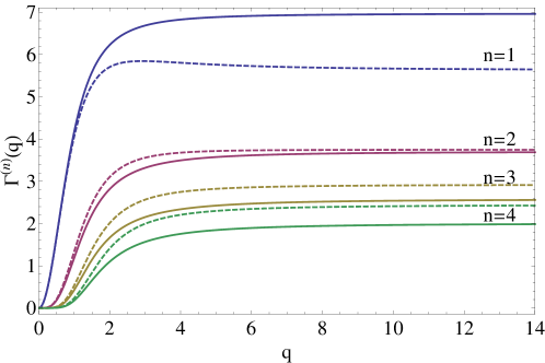
Figure 1: The function $\Gamma^{(n)}(q)$ found by numerical integration for linear (solid lines) and circular (dashed lines) polarization, for n=1,…,4, from top to bottom.

For $q\rightarrow 0$, both linear and circular polarizations yield similar values of $\Gamma^{(n)}(q)$. In that limit, the agreement between the curves corresponding to different polarizations is better as $n$ gets reduced (see Fig. 1). This assertion is further confirmed by the lower limit of the analytical representations of $\Gamma^{(n)}(q)$, which are obtained by fitting the curves displayed in Fig. 1 to quotients of polynomials (see appendix A).

Photons scattered from a Gaussian pulse

As noted in [7], in order to find the total number of photons scattered from a realistic pulse, it is crucial to take into account its finite transverse profile. The previous results for plane waves are useful since, in the spirit of the slowly-varying envelope approximation introduced in section 2.1, a suitable Gaussian profile can be considered, locally, as plane.

The number of photons scattered from a Gaussian pulse is given by an integral of the plane wave result over the non-trivial profile, namely $N_{\gamma}^{(n)}=n_{e}\int N_{\gamma,pw}^{(n)}(q)d^{3}\vec{x}$, where $n_{e}$ is the number of electrons per unit volume and $N_{\gamma,pw}^{(n)}(q)$ is given in Eq. (11). The parameter $q$ depends on the point of space according to Eq. (3). Using the coordinates $\rho,\xi$ defined at the beginning of this section, we can write:

$$N_{\gamma}^{(n)}={\cal K}\int_{-\infty}^{\infty}\int_{0}^{\infty}\rho\,\Gamma^{(n)}(q)d\rho d\xi,$$ (13)

where ${\cal K}$ is a dimensionless quantity,

$${\cal K}=\frac{1}{2}n_{e}\,c\,\tau\,\pi^{2}w_{0}^{4}\lambda_{0}^{-2}\alpha,$$ (14)

where $\alpha=e^{2}/4\pi\,\epsilon_{0}\hbar c\approx 1/137$ is the fine structure constant. Notice that $N_{\gamma}^{(n)}/{\cal K}$ depends only on $n$ and $q_{0}$, and can be straightforwardly computed numerically.

As shown in [7], $N_{\gamma}^{(n)}/{\cal K}$ grows as $q_{0}^{3}\sim I_{0}^{\frac{3}{2}}\sim w_{0}^{-3}$ for large values of the laser peak intensity. Thus, if the remaining parameters are fixed, the number of scattered photons grows linearly with the beam waist radius $w_{0}$ (for small enough $w_{0}$). This behaviour changes for large $w_{0}$ when the intensities are low so that harmonic production is suppressed. In fact, just considering the asymptotic behaviour $\Gamma^{(n)}\propto q^{2n}$ for small values of $q$, we readily find that the integrand in Eq. (13) is proportional to $q_{0}^{2n}\propto w_{0}^{-2n}$. Taking into account the factor ${\cal K}$, we conclude that $N_{\gamma}^{(n)}\propto w_{0}^{4-2n}$ for large $w_{0}$. This asymptotic dependence holds independently of the chosen polarization. These rough arguments qualitatively explain the behaviour depicted in Fig. 2, where a sample numerical computation of the number of scattered photons $N_{\gamma}^{(n)}$ as a function of the beam waist is shown. In particular, the number of photons produced in the second harmonic $n=2$ tends to a constant value, i.e., they do not display any further dependence on $w_{0}$ for large waists. For higher harmonics $n\geq 3$, the signal drops with increasing $w_{0}$, as predicted by the analysis developed in this section. The situation for $n=1$ is subtler since the integral in Eq. (13) diverges in this case. It is plain that such result is not physical since the scattering region is always limited. For the plots included in Fig. 2, the integral has been cut at $q=0.01$, the value associated to the barrier suppression regime, below which the electron of a hydrogen atom cannot be approximated as free any more (for $\lambda_{0}=800$nm) [18]. As we can appreciate from the figure, $N_{\gamma}^{(1)}$ grows monotonically with $w_{0}$.

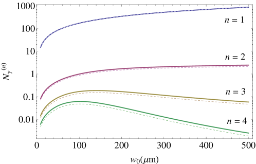
Figure 2: The number of scattered photons from a Gaussian pulse as a function of the beam waist. The following parameters have been fixed for the laser beam $E_{pulse}=30$J, $\tau=30$fs, $\lambda=800$nm. The pressure has been fixed to $p=0.5\times 10^{-11}$Pa and the temperature to $T=300K$ such that $n_{e}=2p/k_{B}T\approx 2.4$mm^-3, where the factor of 2 comes from considering molecular hydrogen with two electrons per molecule. The y-axis (x-axis) is given in logarithmic (linear) scale.

From the figure, we might be tempted to conclude that the optimal value of $w_{0}$ for the measurement of tiny pressures by detecting harmonic-$n$ photons would be the one in which $N_{\gamma}^{(n)}$ reaches its maximum. Nevertheless, this statement is naive for at least three reasons. First, it could prove costly or unfeasible to manipulate ultra-high power pulses in order to achieve too large waists. Second, the larger the $w_{0}$, the larger the region in which the vacuum gauging is taking place. In a chamber with differential vacuum, it would be impossible to measure the vacuum confined in a small region if $w_{0}$ is too large. Third, producing more photons does not mean that a larger signal can be measured. If the region where the scattering is taking place is extensive, it might be impossible to set up an efficient system to collect the emitted photons. We will turn to these questions in section 3.

Non-trivial time envelope

Let us comment on the effect of considering a more realistic non-trivial time envelope instead of a sharp rectangular pulse. We will show that the number of scattered photons does only depend mildly on the envelope and the (simpler) computations of the previous subsections capture the quantitative results up to a factor of order $1$. To take into account the time envelope, we describe the spatio-temporal dependent intensity as $I_{te}=g(\tilde{t})I$, where $I$ is given in Eq. (1) and $t$ should be understood as $\tilde{t}=t-z/c$. If the time envelope varies mildly within a light cycle ($\frac{dg}{d\tilde{t}}\ll\omega g$), a slowly-varying envelope approximation is valid [19] and we may simply use the expression above by including time dependence in $q$. It is useful to define a time envelope correction parameter as the quotient

$$\kappa\equiv\frac{N_{\gamma}^{(n)}|_{te}}{N_{\gamma}^{(n)}|_{ss}}=\frac{\int\rho\,\Gamma^{(n)}\left(\sqrt{g(\tilde{t})}q(\rho,\xi)\right)d\tilde{t}\,d\rho\,d\xi}{\tau\,\int\rho\,\Gamma^{(n)}\left(q(\rho,\xi)\right)d\rho\,d\xi},$$ (15)

where $N_{\gamma}^{(n)}|_{ss}$ refers to the computation with a sharp step time envelope, as in section 2.3. Given the form of the time envelope, $\kappa$ only depends on $q_{0}$ and $n$. As examples, let us consider a Gaussian $g(\tilde{t})=e^{-\pi\tilde{t}^{2}/\tau^{2}}$ and a hyperbolic secant $g(\tilde{t})=$ sech$(\pi\,\tilde{t}/\tau)$, chosen such that $g(0)=1$ and $\int_{-\infty}^{\infty}g(\tilde{t})d\tilde{t}=\tau$. In figure 3, the value of $\kappa$ as a function of $q_{0}$ is plotted for these two time envelopes and for different harmonics, considering linear polarization. The plots for circular polarization are not shown since they are practically coincident with the linear polarization ones.

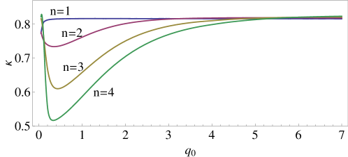
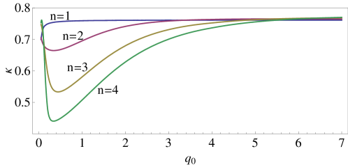
Figure 3: Multiplicative correction due to non-trivial time envelopes to the number of scattered photons as a function of $q_{0}$. On top, the result for the Gaussian envelope and below for hyperbolic secant envelope.

The conclusion is that the sharp step envelope overestimates the number of scattered photons by a factor of order $1$. The correction factors depend on the shape of the actual envelope, the harmonic number and the peak intensity, with typical values around $0.7$ or $0.8$ (see Fig. 3).

Photon collection and geometric efficiency

Up to now, we have computed how many photons are scattered from a given pulse traversing a vacuum chamber. In this section, we will discuss how many might be actually measured in a realistic experiment. Since, in any case, the signal from XHV will be very low, it is essential to use single-photon detectors, which can achieve remarkable quantum efficiencies with state-of-art technology [20, 21]. Typically, the size of the active region of this kind of detectors is of the order of a few microns. Then, since the Thomson scattered photons have a wide angular distribution [7], it is essential to introduce a suitable optical system in order to have efficient photon collection.

The situation is analogous to the detection of Hyper-Rayleigh scattering, a well-established technique for the characterization of nonlinear optical properties of different materials, in particular molecular hyperpolarizabilities [22]: a laser beam traverses the substance to be studied producing anisotropic faint radiation in a multiple of the incident frequency (usually, incoherent second harmonic) which can be collected and measured by an optical system which concentrates part of the emitted light into a photomultiplier. The typical photon collection system — see for instance [23] — is schematically depicted in Fig. 4. As it can be appreciated in the figure, a parabolic mirror captures the photons that are counter-scattered with respect to the position of the single-photon detector, thus enhancing the signal accordingly. An optical system made by filters and lenses allows then to couple most of the scattered light into the detector. A similar arrangement may be used for the measurement of nonlinear Thomson photons in a vacuum chamber.

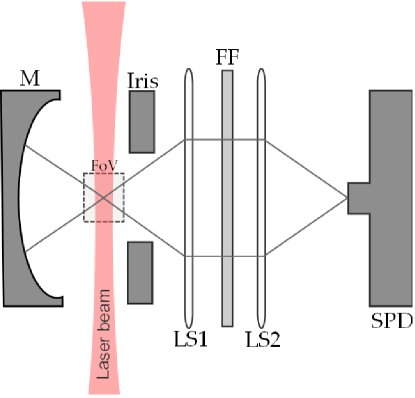
Figure 4: Sketch of a typical scheme for an efficient photon collection system. M: concave mirror, FoV: field of view, FF: frequency filter, LS1, LS2: lens systems, SPD: single-photon detector.

The scheme of Fig.4 is the simplest one can envision, but it may be possible to upgrade it in order to increase the efficiency and/or anticipate possible problems. One possibility is to include a second device like the one in the figure at a different angle in the transverse plane. Another option is to include a multi-mode optical fiber in order to couple the outcome of the optical system to the photon detector. This would allow to place the photon counter away from the experimental zone in order to shield it from eventual secondary radiation, e.g., X-rays, and to reduce undesired background.

Hereafter, we will assume that the optical system can be parametrized by its field of view (FoV), namely, the size of the $z$-region from which scattered photons can be collected, and its numerical aperture (NA), which provides an angular cut for the photons entering the optical system. We also assume that the depth of field (DOF), namely the size of the region that is transverse to the laser beam in the direction of the photon-collecting lens system, does not restrict the detected signal. This approximation is justified if DOF $\gg w_{0}$. We stress that it is only necessary to count the number of photons and not to resolve the location where they were originated.

The field of view and geometric efficiency

Only a fraction of the photons given in Eq. (13) are scattered inside the FoV of the detection system. Assuming that the center of the active detection region coincides with the beam focus, we obtain

$$N_{\gamma,FoV}^{(n)}={\cal K}\int_{-\xi_{m}}^{\xi_{m}}\int_{0}^{\infty}\rho\,{\Gamma}^{(n)}(q)d\rho d\xi.$$ (16)

The integration in $\rho$ is still formally taken up to infinity since typically the beam is concentrated in a submillimeter region in the transverse plane which is assumed to be within the DOF of the collection system in that direction. Our goal in this section is to estimate the geometric efficiency factor associated to the finiteness of the FoV $N_{\gamma,FoV}^{(n)}/N_{\gamma}^{(n)}$ and to discuss the role of $w_{0}$. Notice that $w_{0}$ enters the expression in Eq. (16) in three different ways: in the expression of ${\cal K}$ (recall Eq. (14)), in the value of $q_{0}$ which affects $q$ through Eq. (2) and in the value of the limit value of the integral $\xi_{m}=z_{m}/z_{R}=z_{m}\lambda_{0}/\pi w_{0}^{2}$ where $z_{m}$ is half the FoV. Two examples of the numerically computed value of $N_{\gamma,FoV}^{(n)}$ as a function of $w_{0}$ are presented in Fig. 5.

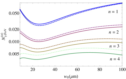
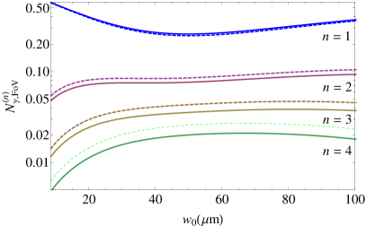
Figure 5: The number of scattered photons within the region $z\in(-z_{m},z_{m})$ from a Gaussian pulse as a function of the beam waist. The parameters of the laser beam and $n_{e}$ are fixed as in Fig. 2. The plot on the left corresponds to $z_{m}=5$mm and the one on the right to $z_{m}=20$mm. Again, the solid lines correspond to linear polarization and the dashed lines to circular polarization. The y-axis (x-axis) is given in logarithmic (linear) scale.

As compared to Fig. 2, we can observe that the dependence of $N_{\gamma,FoV}^{(n)}$ on $w_{0}$ is much milder than that of $N_{\gamma}^{(n)}$. Qualitatively, this can be understood as follows for $n>1$: for moderate values of $w_{0}$, the integral in Eq. (13) is, roughly, proportional to $q_{0}^{3}\propto w_{0}^{-3}$ (multiplying by the prefactor ${\cal K}\propto w_{0}^{4}$, we find $N_{\gamma}^{(n)}\propto w_{0}$). The reason is that the integral is proportional to the volume (in $\rho-\xi$ coordinates) of the region where significant dispersion takes place. The limiting values of $\xi$ and $\rho$ are proportional to $q_{0}$ and thus the volume is proportional to $q_{0}^{3}$ [7]. When the integral is cut as in Eq. (16) and $\xi_{m}$ lies within the significant dispersion region, the integral in $\rho$ still picks up a $q_{0}^{2}\propto w_{0}^{-2}$ factor and the integral in $\xi$ is roughly proportional to $\xi_{m}\propto z_{R}^{-1}\propto w_{0}^{-2}$. Thus, the $w_{0}^{4}$ in ${\cal K}$ cancels out the $w_{0}^{-4}$ from the integral and the dependence of $N_{\gamma,FoV}^{(n)}$ on $\omega_{0}$ is approximately flat. When $w_{0}$ is very small, however, $\xi_{m}$ becomes very large meaning that the region where $q$ is large enough to have significant harmonic production is very small and is comprised within $\xi<\xi_{m}$. Then $N_{\gamma,FoV}^{(n)}\propto w_{0}$ for small $w_{0}$. This can be appreciated in the plot of the right in Fig. 5.

Finally, it is interesting to plot the fraction of photons which are indeed scattered within the FoV of the detection system, namely the geometric efficiency associated to the FoV,

$$\epsilon_{FoV}^{(n)}=\frac{N_{\gamma,FoV}^{(n)}}{N_{\gamma}^{(n)}}.$$ (17)

Notice that this is just the quotient of the quantities plotted in Fig. 5 and Fig. 2. A sample computation is displayed in Fig. 6. The fraction is larger for higher harmonics because the scattering region gets more and more concentrated around the beam focus.

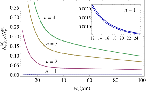
Figure 6: Fraction of photons scattered within the FoV. The physical parameter are those of Fig. 2 together with $z_{m}=5$mm. The region $w_{0}<25\mu$m is enlarged for $n=1$ in the inset.

This plot permits to give an order of magnitude for one of the factors entering the geometric efficiency. For instance, for $n=2$, $w_{0}=15\mu$m with $E_{pulse}=30$J, $\tau=30$fs, $\lambda_{0}=800$nm, FoV=10mm, a 10% photons are scattered from the region from which they do enter the light-collection system. Obviously, this depends strongly on the FoV itself, see Fig. 5.

For simplicity, up to now we have assumed the center of the photon collection system to be at $\xi=0$. However, as a direct consequence of considering the evolution of the Gaussian beam profile, this is not always the optimal choice. In order to get some qualitative insight, let us model (for $n>1$) $\Gamma^{(n)}(q)\approx b_{n}\Theta(q-q_{step,n})$ where $b_{n},q_{step,n}$ are constants and $\Theta(x)$ is Heaviside function. Then, it is straightforward to check that the quantity $\int_{0}^{\infty}\rho\,{\Gamma}^{(n)}(q)d\rho$ has two maxima at $\xi_{c}\approx\pm\sqrt{\frac{q_{0}^{2}}{e\,q_{step,n}^{2}-1}}$. This simple argument qualitatively captures the behaviour depicted in Fig. 7, which can be found by direct numerical integration.

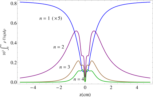
Figure 7: Distribution along the longitudinal direction $z$ of the scattered radiation. The plot has been made taking $E_{pulse}=30$J, $\lambda_{0}=800$nm, $\tau=30$fs, $w_{0}=15\mu$m. In order to present all plots in the same graph, the $n=1$ profile was divided by 5.

By placing the detection system around the corresponding $\xi_{c}$, we obtain

$$N_{\gamma,FoV}^{(n)}={\cal K}\int_{\xi_{c}-\xi_{m}}^{\xi_{c}+\xi_{m}}\int_{0}^{\infty}\rho\,{\Gamma}^{(n)}(q)d\rho d\xi,$$ (18)

which is in general larger than the expression of Eq. (16). Thus, by appropriately displacing the detection system with respect to the beam focus, the geometric efficiency factor can be increased to some extent. We have performed an analysis of an example, using the actual values of $\Gamma^{(n)}(q)$. The results showing the optimal value of $z_{c}=\xi_{c}\pi w_{0}^{2}/\lambda_{0}$ and the increase in the geometric efficiency as compared to Fig. 5 are displayed in Fig. 8.

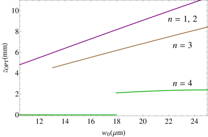
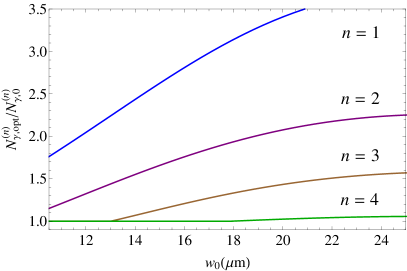
Figure 8: Left: Optimal value of $z_{c}$ for the different harmonics as a function of the waist radius. Right: Plot of the factor by which efficiency is increased, as compared to placing the detector centered around $z=0$. Parameters are as in Figs. 2, 6.

Formally, for $n=1$, the optimal value of $z$ would be $z_{c}\rightarrow\infty$, since the associated profile asymptotes to a constant in Fig. 7. However, for convenience, $z_{c}$ corresponding to $n=1$ will be taken to coincide with that for $n=2$. On the other hand, the discontinuities exhibited by the curves $n=3,4$ in Fig. 8 can be explained by the following argument. The displacement of the detector is useful to capture one of the bumps of the radiation distribution, as shown in Fig. 7. However, when the bumps for both positive and negative values of $z$ come close enough and, as a consequence, can be included within the FoV of the detector, the optimal choice is simply to take $z_{c}=0$. In particular, for a FoV$=10$mm, that would be the case of the $n=4$ lines of Fig. 7.

The optimized geometric efficiency associated to the FoV is then given by the result of Fig. 6 multiplied by the enhancement factor that can be achieved by displacing the detector with respect to the focus (see Fig. 8). For instance, let us consider a laser featuring $E_{pulse}=30$J, $\tau=30$fs, $\lambda=800$nm $w_{0}=15\mu$m and a detector with FoV=10mm. For such a system, the efficiency for the collection of $n=2$ photons would then be optimum (e.g., $\epsilon_{FoV}^{(2)}\approx 0.16$ in this particular case) for $z_{c}=6.85$mm.

Numerical aperture. Angular acceptance

Among all photons coming from the FoV, only those within certain angular cuts are effectively captured by the collection system. The quantity defining the angular acceptance of the optical system is NA. Assuming that the refractive index of the medium is 1, it is defined as NA $=\sin\tilde{\theta}_{i}$, such that the radiation with $\tilde{\theta}<\tilde{\theta}_{i}$ is measured. $\tilde{\theta}$ is defined as the angle between the photon direction and the axis joining the scattering region to the center of the optical system and thus is not the $\theta$ used in the previous sections. The goal of this section is to estimate the fraction of scattered photons lying within the NA, thus finding the corresponding factor for the geometric efficiency of the photon collection system.

The number of photons scattered per unit solid angle by a Gaussian beam traversing a vacuum chamber is easily derived from the expressions given in section 2,

$$\frac{dN_{\gamma}^{(n)}}{d\Omega}={\cal K}\int_{-\infty}^{\infty}\int_{0}^{\infty}\frac{1}{n}\rho{\cal M}f^{(n)}d\rho d\xi.$$ (19)

The efficiency associated to the numerical aperture would then be

$$\epsilon_{NA}^{(n)}=\frac{2\int_{\tilde{\theta}<\tilde{\theta}_{i}}\left(dN_{\gamma}^{(n)}/d\Omega\right)d\Omega}{\int_{\Omega}\left(dN_{\gamma}^{(n)}/d\Omega\right)d\Omega},$$ (20)

where the integral in the denominator is taken over the full solid angle. The factor of 2 in the numerator comes from considering both the integrals in $\tilde{\theta}\in[0,\tilde{\theta}_{i}]$ and in $\tilde{\theta}\in[\pi-\tilde{\theta}_{i},\pi]$ because of the mirror placed opposite to the detector (see Fig. 4).

The expression Eq. (20) can be directly evaluated numerically in any particular case. In fact, we have verified that the angular distribution of Eq. (19) is rather accurately approximated by the low $q$ angular dependence of the integrand. We can then obtain a simple estimate of $\epsilon_{NA}^{(n)}$, depending only on the polarization state, the harmonic number, and the numerical aperture. Defining

$$\Xi^{(n)}(\theta,\varphi)\equiv\frac{1}{n}\lim_{q\to 0}\frac{f^{(n)}}{q^{2n}},$$ (21)

Eq. (20) reads

$$\epsilon_{NA}^{(n)}\approx\frac{2\int_{\tilde{\theta}<\tilde{\theta}_{i}}\Xi^{(n)}d\Omega}{\int_{\Omega}\Xi^{(n)}d\Omega}.$$ (22)

The cases of circular and linear polarization are discussed separately below.

Circular polarization

By expanding Eq. (8), we find

$$\Xi_{c}^{(n)}=\frac{2^{2-3n}n^{2n-1}}{(n-1)!}(1+\cos^{2}\theta)(\sin\theta)^{2n-2},$$ (23)

which gives

$$\int_{\Omega}\Xi_{c}^{(n)}d\Omega=\frac{2^{4-n}\pi(1+n)n^{2n}}{(2n+1)!}.$$ (24)

In order to compute the numerator of Eq. (22), let us define a new set of spherical coordinates obtained by a rotation of $\pi/2$ with respect to the $x$-axis,

$$\cos\theta = \sin\tilde{\theta}\sin\tilde{\varphi}\,\,,$$

$$\tan\varphi = -\cot\tilde{\theta}\sec\tilde{\varphi}\,.$$ (25)

This amounts to placing the detection system ($\tilde{\theta}=0$) along the $y$-axis. By inserting the expression given in Eq. (25) into Eq. (23) and Eq. (22), estimates for $\epsilon_{NA}^{(n)}$ can be found. For instance, if $NA=0.5$, meaning $\tilde{\theta}_{i}=\pi/6$, we obtain $\epsilon_{NA}^{(1)}\approx 0.11$, $\epsilon_{NA}^{(2)}\approx 0.17$, $\epsilon_{NA}^{(3)}\approx 0.20$, $\epsilon_{NA}^{(4)}\approx 0.23$.

Linear polarization

This case is more complicated than the previous one because of the $\varphi$-dependence of the differential cross section and the cumbersome form of Eq. (7). The angle $\beta$ between the polarization direction and the location of the detector has to be properly chosen. All computational details are relegated to appendix B, whereas only the estimates of the geometric efficiency factor related to angular acceptance are quoted here. Assuming NA=0.5, namely $\tilde{\theta}_{i}=\pi/6$, they are $\epsilon_{NA}^{(1)}\approx 0.19$, $\epsilon_{NA}^{(2)}\approx 0.19$, $\epsilon_{NA}^{(3)}\approx 0.31$ and $\epsilon_{NA}^{(4)}\approx 0.49$. Notice that they are larger than the efficiencies that can be achieved with circular polarization. This is due to the breaking of the azimuthal symmetry, implying that the distribution of scattered power is more inhomogeneous over the solid angle. We can profit from this fact by suitably choosing the location of the photon collection system.

Summary and an example

Let us summarize the main results of section 3. Once given the characteristics of a laser pulse ($E_{pulse}$, $\tau$, $\lambda_{0}$) and of a photon collection system (its FoV and NA), the waist radius of the beam and the position of the detector, both in the longitudinal direction $z_{c}$ and its angular position in the transverse plane $\beta$ can be optimized. In section 3.2 and appendix B, we give an estimate of the optimal $\beta$ and the efficiency associated to the angular acceptance. Section 3.1 discusses how to choose values of $w_{0}$ and $z_{c}$ and gives the quantitative results for the geometric efficiency associated to the FoV in a sample case. It does not seem possible to provide a simple estimate for these quantities as a function of all the input parameters.

It is worth mentioning that the full geometric efficiency is not exactly the product of $\epsilon_{FoV}$ and $\epsilon_{NA}$ since, in an actual computation, both cuts should be taken into account simultaneously. However, we have discussed their computations separately for clarity of exposition. In any case, the error we make by splitting the computation in this fashion is not large, although it depends on the particular case. For instance, for the quoted case with linear polarization with $E_{pulse}=30$J, $\tau=30$fs, $\lambda=800$nm, FoV = 10mm, $w_{0}=15\mu$m, $z_{c}=6.85$mm, $NA=0.5$, $\beta=0.84$ the efficiencies given above are $\epsilon_{FoV}^{(2)}=0.163$ and $\epsilon_{NA}^{(2)}=0.19$, such that $\epsilon_{FoV}^{(2)}\epsilon_{NA}^{(2)}=0.031$. This should be compared with the computation including directly in the integrals both cuts which gives $\epsilon_{geom}=0.030$.

Some quantitative estimates

One of the conclusions of the previous sections is that the beam polarization affects only mildly the number of scattered photons, see Figs. 2-8. In contrast, it modifies more severely the angular distribution of radiation and, therefore, the number of photons that propagate within the numerical aperture of the detector. This distribution is more inhomogeneous for linear polarization and this fact permits to enhance the geometric efficiency by suitably placing the detection system, see section 3.2. In the following we will concentrate on linear polarization. It was shown in [7] that in this case the number of scattered photons per pulse is $N_{\gamma}^{(n)}\approx c_{n}{\cal K}\,q_{0}^{3}$ where the $c_{n}$ are coefficients that can be computed numerically, $c_{1}\approx 275$, $c_{2}\approx 1.3$, $c_{3}\approx 0.22$, $c_{4}\approx 0.088$. This expression is valid for large $q_{0}$, corresponding to the region of small $w_{0}$ in Fig. 2, in which $N_{\gamma}^{(n)}\propto w_{0}$. A laser with repetition rate $r_{r}$ operating for a time interval $\Delta t$ produces $\Delta t\,r_{r}$ pulses. Under conditions of XHV, the number of detected photons is proportional to the electron density:

$$N_{\gamma,det}^{(n)}={\cal A}\,n_{e}.$$ (26)

The value of the proportionality constant can be found by substituting the values for ${\cal K}$ and $q_{0}$ in the expression for $N_{\gamma}^{(n)}$ given above [7], so that

$${\cal A}\approx\frac{4c_{n}}{\pi}(\Delta t\,r_{r})\alpha\,\frac{w_{0}\lambda_{0}r_{0}^{3/2}}{(c\,\tau)^{\frac{1}{2}}}\left(\frac{E_{pulse}}{m_{e}c^{2}}\right)^{\frac{3}{2}}f\,\kappa\,.$$ (27)

The parameter $\kappa$ is the correction due to a non-trivial time envelope and will be fixed to a typical value 0.8, see section 2.4. The efficiency factor $f\approx\epsilon_{geom}\epsilon_{q}\epsilon_{\lambda}$ is the efficiency factor including the geometric efficiency (see section 3), the quantum efficiency of the detector and the cuts imposed by the frequency filter.

Furthermore, $n_{e}$ is proportional to the pressure,

$$n_{e}=\eta\frac{p}{k_{B}T},$$ (28)

where $\eta$ is the average number of weakly bound electrons per molecule [7] — namely, those in the barrier suppression regime. It depends on the atomic and molecular composition of the remnant gas in the vacuum chamber. In a canonical XHV, its value would be $\eta\approx 2$ since it is mostly composed of hydrogen molecules [24, 25].

The goal of this section is to provide estimates of these quantities for three PW facilities that will be available in the near future, namely VEGA [26], JuSPARC [27, 28], and a 10 PW branch of the ELI project [29], which have been chosen because of their sizable repetition rates, see table 1.

Facility	$P_{p}$ (PW)	$E_{pulse}$ (J)	$\tau$ (fs)	$\lambda_{0}$ (nm)	$r_{r}$ (Hz)
VEGA	1	30	30	800	1
JuSPARC	1.5	45	30	800	1
ELI 10 PW	10	300	30	800	0.1

Table 1: A few facilities that will operate in the near future.

In all cases, we will assume band-pass filters for each harmonic as $\lambda_{1}$(nm) $\in[800,1200]$, $\lambda_{2}$(nm) $\in[400,800]$, $\lambda_{3}$(nm) $\in[267,400]$, $\lambda_{4}$(nm) $\in[200,267]$ (recall that the photon wavelength is shifted by a $q$-dependent factor, Eq. (10)). This choice should be adjusted for a particular detector and frequency filter, see an enlarged discussion in section 5. We consider an experiment running for $\Delta t=$ 1 day. A detection system with FoV = 10mm, NA = 0.5 and an average quantum efficiency of $\epsilon_{q}=0.25$ within the allowed wavelength bands will be considered. These are sample values intended to be representative and to provide a reasonable estimate for realistic situations.

The results are summarized in table 2. Harmonics $n=1,\dots,4$ are considered in each case, the position of the detector along $z$ is optimized as explained in section 3.1 and the angle $\beta$ is chosen in each case as in appendix B. The waist radii, chosen to comply with (4), are taken to be $w_{0}=15\mu$m, $w_{0}=15\mu$m, $w_{0}=27.5\mu$m for VEGA, JuSPARC and ELI 10, respectively, ($q_{0}\approx 11.5$, $q_{0}\approx 14.1$, $q_{0}\approx 19.8$). The efficiency factors $\epsilon_{geom}$, $\epsilon_{\lambda}$ and the proportionality factor ${\cal A}$ of equations (26), (27) are found by computing the appropriate numerical integrals.

Facility	n	$z_{c}$ (mm)	$\epsilon_{geom}$	$\epsilon_{\lambda}$	${\cal A}$ (mm3)
VEGA	1	6.85	$6.5\times 10^{-4}$	0.94	113
	2	6.85	$3.0\times 10^{-2}$	0.96	25
	3	5.2	$7.2\times 10^{-2}$	0.68	7.6
	4	0	$9.6\times 10^{-2}$	0.16	0.9
JuSPARC	1	8.4	$5.4\times 10^{-4}$	0.94	172
	2	8.4	$2.6\times 10^{-2}$	0.97	41
	3	6.4	$6.8\times 10^{-2}$	0.65	12
	4	2.35	$7.2\times 10^{-2}$	0.19	1.5
ELI 10	1	4.35	$1.2\times 10^{-4}$	0.95	122
	2	4.35	$6.2\times 10^{-3}$	1.0	32
	3	3.3	$1.8\times 10^{-2}$	0.53	8.4
	4	1.25	$1.1\times 10^{-2}$	0.12	0.46

Table 2: Estimates for three future facilities.

The first observation is that, even if the geometric efficiency is much lower for $n=1$, the majority of photons reaching the detector are of this fundamental harmonic. Nevertheless, the difference is less than one order of magnitude with respect to $n=2$. Gauging the pressure by looking at this second harmonic would have several assets: it would help to avoid possible undesired background of photons from the main beam reaching the detector without having been ’Thomson scattered’ and also to reduce other sources of background such as thermal noise. Moreover, photon detectors typically reach higher quantum efficiencies with smaller dark counts in the visible than in the IR, although that can depend on the detector itself, see [30] for a review of single photon detectors. Recall that in table 2, the same quantum efficiency was assumed in all cases. On the other hand, the separate measurement of both the $n=1$ and $n=2$ harmonics can be used to self-calibrate the procedure.

Let us first estimate the minimum pressure that could be gauged, in principle, in a one day experiment at the three mentioned facilities by detecting the $n=1$ photons. Since extreme vacuum is mostly formed by molecular hydrogen, we take $\eta=2$ in Eq. (28). We require that the average number of photons measured in the detection period is at least 10. Then $p_{min}\approx 10k_{B}T/(2{\cal A})$, where the values of ${\cal A}$ are given in table 2. For VEGA, we obtain $p_{min}\approx 1.8\times 10^{-13}$Pa at room temperature $T=300$K or $p_{min}\approx 2.3\times 10^{-15}$Pa at liquid He temperature $T=4$K. For JuSPARC, $p_{min}\approx 1.2\times 10^{-13}$Pa at $T=300$K or $p_{min}\approx 1.5\times 10^{-15}$Pa at $T=4$K. For ELI 10, $p_{min}\approx 1.6\times 10^{-13}$Pa at $T=300$K or $p_{min}\approx 2.2\times 10^{-15}$Pa at $T=4$K. It should be noted that these results may be improved, leading to the possible measurement of even lower pressures, by using a different setup allowing for a greater geometric efficiency. The theoretical limit can be found by multiplying the results of Ref. [7] including the time envelop correction that we have computed above. In any case, the optimization procedure that we have developed above can be straightforwardly generalized to any given geometry.

Let us consider the case in which the second harmonic, $n=2$, is used to gauge the vacuum, and find the estimates of the minimum pressure that could be gauged in one day in the three mentioned facilities. For VEGA, we obtain $p_{min}\approx 8\times 10^{-13}$Pa at room temperature $T=300$K or $p_{min}\approx 1.1\times 10^{-14}$Pa at liquid He temperature $T=4$K. For JuSPARC, $p_{min}\approx 5\times 10^{-13}$Pa at $T=300$K or $p_{min}\approx 0.7\times 10^{-14}$Pa at $T=4$K. For ELI 10, $p_{min}\approx 6.5\times 10^{-13}$Pa at $T=300$K or $p_{min}\approx 0.9\times 10^{-14}$Pa at $T=4$K.

Discussion

In this section, a few interesting questions that have been left out of the general discussion are addressed.

For linear polarization, the trajectory of an electron extracted from an atom by the electromagnetic field passes near the ion during its oscillation, opening the possibility of electron-nucleus recombination with the associated photon emission. This harmonic-generating phenomenon has not been taken into account in the discussion. The safest possibility is to introduce a slight ellipticity in the beam polarization in order to reduce the probability of this circumstance to happen, while keeping nearly unchanged the angular distribution of the Thomson radiation.

We have discussed the minimum pressure that can be gauged in a given situation, associated to having a detectable signal of photons. Another interesting question is which would be the maximum measurable pressure. The method presented in this note would be useful as long as the pressure and the number of scattered photons remain proportional to each other. This can only break down when the density of active electrons is high enough to introduce collective effects. A extremely conservative estimate would be to compare the volume per electron ($n_{e}^{-1}=k_{B}T/\eta p$) to the volume of the laser pulse (roughly $\frac{\pi}{2}w_{0}^{2}c\,\tau$). Taking values $w_{0}=15\mu$m, $\tau=30$fs, $T=300$K, $\eta=2$ gives $p\approx 10^{-6}$Pa. This value is in the so-called high vacuum regime in which pressure can be measured with great precision with standard techniques. In fact, comparing in this regime laser measurements with standard ones would be a valuable benchmark calibration of the method.

It is conceivable to design ultra-high or extreme vacuum gauges using table-top terawatt lasers rather than PW facilities. These could find more applications since the cost of the required device would be orders of magnitude lower. The reduced power would be compensated, at least partially, by larger repetition rates. However, even if the general idea presented here would hold, the actual computations would not. For beams far from the diffraction limit, terawatt lasers would yield $q_{0}<1$, i.e., intensities out of the relativistic regime. For instance, with $P_{p}=3$TW, $w_{0}=15\mu$m, $\lambda_{0}=800$nm, we obtain $q_{0}^{2}\approx 0.4$. Harmonic production would be suppressed and expressions like Eqs. (26)-(27) would fail. Moreover, for pulse durations down to the few-cycle limit, the approximation of slowly-varying envelope considered throughout this paper would no longer hold — see for instance [31]. The exploration of such limiting case, although interesting, lies beyond the scope of the present work.

Finally, it is worth discussing the wavelength spectrum of the scattered photons. In laboratory frame, the spectral distribution that can be computed with the expression used above is rather broad [7]. It would be further broadened by at least two additional effects which are enhanced for short pulses: the width of the incoming laser pulse itself and the departure from the results of [14] when the envelope is not slowly-varying [32, 33]. The spectra for the different harmonics can be overlapping, producing a sort of supercontinuum. In fact, splitting the results in harmonics is just a convenient computational artifact, while the physical measurable result is the sum of all them. In that sense, the results presented in table 2 are lower limits since they only include the first (larger) contribution in the harmonic sum for the different wavelength bands. Notice that this overlap is harmless for the proposed pressure gauge since the total signal remains proportional to the number of scattering electrons. It is obvious that photon detectors with broad efficiency curves would be necessary. Once given a curve in a particular case, the computations shown above can be generalized by properly including it in the integrals, instead of assuming a constant quantum efficiency and a sharp band-pass filter.

Conclusions

The availability of ultra-short and ultra-intense laser pulses opens the possibility of gauging extreme vacuum pressure by photon counting. The huge photon concentration in these pulses allows to overcome, in the long run, the scantiness of scattering centers in extremely rarefied gases. The shortness of the pulses allows to synchronize the measurements with the pulse passage and to eliminate (or, at least, dramatically reduce) the undesired background by gating in time the signal produced by the photon detectors. Moreover, for the high intensities that can be obtained with focused PW laser beams corresponding to $q\gtrsim 1$, a significant quantity of radiation is non-linearly Thomson-scattered in harmonics $n>1$. The selective detection of only these higher harmonics can be used to significantly reduce any possible background coming from the possible deviations of the original beam from the axially-centered Gaussian distribution. We have considered a typical photon collection system and shown how to optimize the vacuum gauge accuracy by properly placing the detectors. Within this realistic setup, we have obtained optimized geometric efficiencies of the order of a few percent for $n>1$. We have also shown that these results hold for any choice of polarization of the incoming pulse, with numerical variations of the order of the unity. With these assumptions, pressures of the order of $p=10^{-13}-10^{-12}$ Pa at room temperature can be measured in a one-day experiment at VEGA, JuSPARC or ELI 10, assuming that such conditions can be created and maintained during this time. This same procedure can be also applied to more encompassing dispositions of the detectors, that can lead to greater geometrical efficiencies and may eventually allow to lower the limiting pressure that can be achieved.

Upgrading and understanding the classical vacuum may be crucial for experiments trying to explore properties of the quantum vacuum [4, 5, 6]. Apart from gauging the pressure, nonlinear Thomson scattering might also be useful for beam characterization [32] since its detection can be a probe of the focusing region where it is impossible to introduce any direct characterization system. Har-Shemesh and Di Piazza have proposed to employ it to provide indirect measurements of the peak intensity [34] and, in the same spirit, the possibility of studying beam profiles or time envelopes is worth investigating. Hopefully, the computations presented here could be instrumental in this direction.

Acknowledgements

We thank M. Büscher, D. González-Díaz, J. Hernández-Toro, J. A. Pérez-Hernández, A. Peralta, L. Roso and C. Ruiz for useful discussions. A.P. is supported by the Ramón y Cajal program. D.T. thanks the InterTech group of Valencia Politechnical University for hospitality during a research visit that was supported by the Salvador de Madariaga program of the Spanish Government. The work of A.P. and D.T. is supported by Xunta de Galicia through grant EM2013/002.

Appendix A Approximate expressions for the $\Gamma^{(n)}(q)$

The functions $\Gamma^{(n)}(q)$ defined in section 2.2 are important tools in the computation of the number of photons scattered by the nonlinear Thomson effect. The formal expressions are rather involved and can only be evaluated numerically. Nevertheless, we have checked that they can be well approximated by simple quotients of polynomials for the values of $n$ considered, see Fig. 1. The error of the approximation is under 1% in most of the range and, in fact, plotting the expressions below in Fig. 1 would display lines not distinguishable from the numerical results. Only even powers of $q$ are considered since, formally, $\Gamma^{(n)}(q)=\Gamma^{(n)}(-q)$.

For linear polarization

$$\Gamma^{(1)}_{l}(q) \approx \frac{8\pi}{3}\frac{q^{2}(1+0.414q^{2})}{1+1.33q^{2}+0.497q^{4}}\,\,,$$

$$\Gamma^{(2)}_{l}(q) \approx \frac{7\pi}{5}\frac{q^{4}(1+0.454q^{2})}{1+2.18q^{2}+1.63q^{4}+0.539q^{6}}\,\,,$$

$$\Gamma^{(3)}_{l}(q) \approx \frac{207\pi}{224}\frac{q^{6}}{1+2.97q^{2}+1.66q^{4}+1.13q^{6}}\,\,,$$

$$\Gamma^{(4)}_{l}(q) \approx \frac{1081\pi}{1620}\frac{q^{8}}{1+2.79q^{2}+4.79q^{4}+2.07q^{6}+1.05q^{8}}\,\,.$$

For circular polarization

$$\Gamma^{(1)}_{c}(q) \approx \frac{8\pi}{3}\frac{q^{2}(1+0.249q^{2})}{1+1.20q^{2}+0.370q^{4}}\,\,,$$

$$\Gamma^{(2)}_{c}(q) \approx \frac{8\pi}{5}\frac{q^{4}(1+0.246q^{2})}{1+1.98q^{2}+1.34q^{4}+0.330q^{6}}\,\,,$$

$$\Gamma^{(3)}_{c}(q) \approx \frac{81\pi}{70}\frac{q^{6}(1+0.245q^{2})}{1+2.74q^{2}+2.94q^{4}+1.44q^{6}+0.305q^{8}}\,\,,$$

$$\Gamma^{(4)}_{c}(q) \approx \frac{512\pi}{567}\frac{q^{8}}{1+1.17q^{2}+7.05q^{4}+1.55q^{6}+1.16q^{8}}\,\,.$$

We have taken into account that the leading term of all $\Gamma^{(n)}(q)$ for small $q$ is of order $q^{2n}$. Its coefficient can be straightforwardly computed by Taylor expansion and has been inserted in the expressions above. The rest of coefficients have been fitted to the data found from numerical integrals.

Appendix B Geometric efficiency related to numerical aperture for linear polarization

It is possible to write down explicit expressions for the $\Xi^{(n)}$ defined in Eq. (21) by expanding (7):

$$\Xi_{l}^{(1)} = \sin^{2}\alpha\,\,,$$

$$\Xi_{l}^{(2)} = \cos^{2}\alpha(2\sin^{2}\alpha-\cos\theta)+\frac{1}{8}\sin^{2}\theta\,\,,$$

$$\Xi_{l}^{(3)} = \frac{27}{64}\Big{(}\frac{1}{4}\sin^{2}\alpha(1-\cos\theta-6\cos^{2}\alpha)^{2}+$$

$$+ \sin^{2}\theta\cos^{2}\alpha+\cos\theta\cos^{2}\alpha(1-\cos\theta-6\cos^{2}\alpha)\Big{)}\,\,,$$

$$\Xi_{l}^{(4)} = \sin^{2}\alpha\cos^{2}\alpha(1-\cos\theta-\frac{8}{3}\cos^{2}\alpha)^{2}+$$ (B.1)

$$- \frac{1}{4}\cos\theta\cos^{2}\alpha(1-\cos\theta-\frac{8}{3}\cos^{2}\alpha)$$

$$(1-\cos\theta-8\cos^{2}\alpha)+$$

$$+ \frac{1}{64}\sin^{2}\theta(1-\cos\theta-8\cos^{2}\alpha)^{2}.$$

Equivalent expressions for $n=1,2,3$ were given in [14] with two typos that were corrected in [35].

Since in the case of linear polarization the azimuthal symmetry is broken, it is convenient to choose the angular position of the detection system with respect to the polarization direction in order to optimize the detection of photons. Consider a new set of spherical coordinates by first performing a $\pi/2$-rotation around the $x$-axis followed by a $\beta$-rotation around the new $y$-axis,

$$\theta = \arccos\left(\sin\tilde{\theta}\,\sin\tilde{\varphi}\right)\,\,,$$

$$\varphi = -\arctan\left(\frac{\sin\beta\sin\tilde{\theta}\cos\tilde{\varphi}+\cos\beta\cos\tilde{\theta}}{\cos\beta\sin\tilde{\theta}\cos\tilde{\varphi}-\sin\beta\cos\tilde{\theta}}\right).$$ (B.2)

For $\beta=0$, Eq. (25) is recovered. For a given value of $\beta$ and the numerical aperture $\sin\tilde{\theta}_{i}$, the efficiency (22) can be computed. Then, it is straightforward to find the value of $\beta$ which optimizes $\epsilon_{NA}^{(n)}$ and which indicates where the optical system should be placed. The optimal $\beta$ depends on the harmonic number and also on the numerical aperture. For instance, fixing $NA=0.5$, namely $\tilde{\theta}_{i}=\pi/6$, we find $\beta=0$ for $n=1$, $\beta\approx 0.84$ for $n=2$ and $\beta=\pi/2$ for $n=3$ and $n=4$. The corresponding values of the efficiency are quoted in section 3.2 of the main text. The value $\beta=0$ for $n=1$ could be expected since, for linear Thomson scattering, the maximum of the scattered radiation is emitted perpendicular to the polarization direction. Nevertheless, that is not the case for harmonic generation from nonlinear Thomson scattering.

References

- [1] D. Strickland and G. Mourou, Opt. Commun. 56, 219 (1985).
- [2] V. Yanovsky et al, Opt. Express 16, 2109 (2008).
- [3] G. A. Mourou, T. Tajima, and S. V. Bulanov, Rev. Mod. Phys. 78, 310 (2006).
- [4] M. Marklund, P. K. Shukla, Rev. Mod. Phys. 78, 591 (2006); F. Ehlotzky, K. Krajewska, J. Z. Kaminski, Rep. Prog. Phys. 72, 046401 (2009); A. Di Piazza, C. Muller, K. Z. Hatsagortsyan, and C. H. Keitel, Rev. Mod. Phys. 84, 1177 (2012).
- [5] S. L. Adler, Ann. Phys. 67, 599 (1971); E. B. Aleksandrov, A. A. Anselm, A. N. Moskalev, Sov. Phys. JETP 62, 680 (1985); Y. J. Ding, A. E. Kaplan, Phys. Rev. Lett. 63, 2725 (1989); F. Moulin, D. Bernard, Opt. Comm. 164, 137 (1999); D. Bernard et al., Eur. Phys. J. D 10, 141 (2000); G. Brodin, M. Marklund, L. Stenflo, Phys. Rev. Lett. 87, 171801 (2001); G. Brodin et al. Phys. Lett. A 306, 206 (2003); V. I. Denisov , I. V. Krivchenkov, N. V. Kravtsov, Phys. Rev. D 69, 066008 (2004); T. Heinzl et al., Opt. Comm. 267, 318 (2006); A. Di Piazza, K.Z. Hatsagortsyan, C.H. Keitel, Phys. Rev. Lett. 97, 083603 (2006); A. Ferrando, H. Michinel, M. Seco, D. Tommasini, Phys. Rev. Lett., 99, 150404 (2007); D. Tommasini, A. Ferrando, H. Michinel, M. Seco, Phys. Rev. A 77, 042101 (2008); E. Lundstrom et al., Phys. Rev. Lett. 96, 083602 (2006); M. Marklund, J. Lundin, Eur. Phys. J. D 55, 319 (2009); B. King, A. Di Piazza, and C. H. Keitel, Nat. Photonics 4, 92 (2010); M. Marklund, Nat. Photonics 4, 72 (2010); D. Tommasini, and H. Michinel, Phys. Rev. A 82, 011803R (2010); B. King, A. Di Piazza and C. H. Keitel, Phys. Rev. A 82, 032114 (2010); H. Gies and L. Roessler, Phys. Rev. D 84, 065035 (2011); B. King, C. H. Keitel, New J. Phys. 14, 103002 (2012); Qiang-Lin Hu et al. Phys. of Plasmas 19, 042306 (2012); L. Kovachev, D. A. Georgieva, A. Daniela, K. L. Kovachev, Opt. Lett. 37, 4047 (2012); E. Milotti, et al., Int. J. Quant. Inf. 10, 1241002 (2012); J. K. Koga et al. Phys. Rev. A 86, 053823 (2012); R. Battesti, and C. Rizzo, Rep. Prog. Phys. 76, 016401 (2013).
- [6] M. Bregant et al., PVLAS, Phys. Rev. D 78, 032006 (2008); G. Zavattini and E. Calloni, Eur. Phys. J. C 62, 459 (2009); D. Tommasini, A. Ferrando, H. Michinel, M. Seco, J. High Energy Phys. 11 043 (2009); B. Dobrich, H. Gies, J. High Energy Phys. 10, 022 (2010); A. Accioly, P. Gaete, J. A. Helayel-Neto, Int. J. Mod. Phys. 25, 5951 (2010); B. Doebrich, A. Eichhorn, J. High Energy Phys. 06, 156 (2012); G. Zavattini, et al. Int. J Mod. Phys. 27, 1260017 (2012); B. Dobrich, H. Gies, N. Neitz, F. Karbstein, Phys. Rev. D 87, 025022 (2013); E. Y. Petrov, A. V. Kudrin, Phys. Rev. D 87, 087703 (2013).
- [7] A. Paredes, D. Novoa and D. Tommasini, Phys. Rev. Lett. 109, 253903 (2012).
- [8] P. A. Redhead, Ultrahigh and Extreme High Vacuum, in ”Foundations of Vacuum Science and Technology”, p. 625, Ed. J. M. Lafferty (Wiley, New York) (1998).
- [9] P.A. Redhead, Cern accelerator school vacuum technology, proceedings, Cern reports 99, 213-226 (1999).
- [10] A. Calcatelli, Measurement 46-2, 1029-1039 (2013).
- [11] J. Z. Chen, C. D. Suen and Y.H. Kuo, J. Vac. Sci. Technol. A. 5, 2373 (1987).
- [12] H. Häffner et al., Eur. Phys. J. D 22, 163-182 (2003).
- [13] J.H. Eberly and A. Sleeper, Phys. Rev. 176, 1570 (1968); E. Esarey, S.K. Ride, P. Sprangle, Phys. Rev. E 48, 3003 (1993); S.-Y. Chen, A. Maksimchuk, D. Umstadter, Nature 396, 653 (1998); S.Y. Chen, A. Maksimchuk, E. Esarey, D. Umstadter, Phys. Rev. Lett., 84, 5528 (2000); M. Babzien et al., Phys. Rev. Lett. 96, 054802(2006). T. Kumita et al. Laser Phys. 16, 267 (2006).
- [14] E.S. Sarachik, G.T. Schappert, Phys. Rev. D 1, 2738 (1970).
- [15] Y.I. Salamin, F.H.M. Faisal, Phys. Rev. A 54, 4383 (1996).
- [16] Y.I. Salamin, F.H.M. Faisal, Phys. Rev. A 55, 3694 (1997).
- [17] J. D. Lawson, IEEE Trans. Nucl. Sci. NS-26, 4217 (1979); E. Esarey, C. B. Schroeder, and W. P. Leemans, Rev. Mod. Phys. 81 ,1229 (2009).
- [18] N.B. Delone, V.P. Krainov, Uspekhi Fizicheskikh Nauk 168 (5), 531 (1998); V.V. Strelkov, A.F. Sterjantov, N.Yu Shubin, V.T. Platonenko, J. Phys. B: At. Mol. Opt. Phys. 39, 577 (2006).
- [19] P. Gibbon, Short Pulse Laser Interaction with Matter, Imperial College Press (2007).
- [20] A. Korneev et al., IEEE Trans. Appl. Supercon. 15, 2, 571 (2005).
- [21] K. Smirnov et al., J. Phys.: Conf. Ser. 61, 1081 (2007).
- [22] K. Clays, A. Persoons, Phys. Rev. Let. 66, 2980 (1991); K. Clays, A. Persoons, Rev., Sci. Instrum. 6 3285 (1992); K. Clays, A. Persoons, L. De Maeyer, Adv. Chem. Phys. 85 (III), 455 (1994).
- [23] E. Hendrickx, K. Clays, A. Persoons, Acc. Chem. Res., 31, 675 (1998).
- [24] P. J. Bryant et al., NASA CR-324 (1965).
- [25] J. L. Abelleira-Fernández et al., J. Phys. G: Nucl. Part. Phys. 39 075001 (2012).
- [26] http://www.clpu.es/es/infraestructuras/linea- principal/fase-3.html .
- [27] Annual Report 2011 of the IKP, Berichte des Forschungszentrums Jülich Juel-4349, ISSN: 0944-2952. http:// donald.cc.kfa-juelich.de/wochenplan/publications/ AR2011/documents/AR2011_Highlights.pdf
- [28] M. Büscher, private communication.
- [29] http://www.extreme-light-infraestructure.eu.
- [30] M.D. Eisaman, J. Fan, A. Migdall, S.V. Polyakov, Rev. Sci. Instrum 82 071101 (2011).
- [31] F. Mackenroth, A. Di Piazza, Phys. Rev. A 83, 032106 (2011).
- [32] G.A. Krafft, Phys. Rev. Lett. 92, 204802 (2004).
- [33] J. Gao, Phys. Rev. Lett. 93, 243001 (2004); Y. Tian et al. Opt. Comm. 261, 104 (2006); Y. Tian, Y. Zheng, Y. Lu, J. Yang, Optik 122, 1373 (2011).
- [34] O. Har-Shemesh, A. Di Piazza, Opt. Lett. 37, 1352 (2012).
- [35] C.I. Castillo-Herrera, T.W. Johnston, IEEE Trans. Plasma Sci. 21, 125 (1993).