Snakes and Ladders in an Inhomogeneous Neural Field Model

Abstract

Continuous neural field models with inhomogeneous synaptic connectivities are known to support traveling fronts as well as stable bumps of localized activity. We analyze stationary localized structures in a neural field model with periodic modulation of the synaptic connectivity kernel and find that they are arranged in a snakes-and-ladders bifurcation structure. In the case of Heaviside firing rates, we construct analytically symmetric and asymmetric states and hence derive closed-form expressions for the corresponding bifurcation diagrams. We show that the approach proposed by Beck and co-workers to analyze snaking solutions to the Swift–Hohenberg equation remains valid for the neural field model, even though the corresponding spatial-dynamical formulation is non-autonomous. We investigate how the modulation amplitude affects the bifurcation structure and compare numerical calculations for steep sigmoidal firing rates with analytic predictions valid in the Heaviside limit.

1 Introduction

Continuous neural field models are a common tool to investigate large-scale activity of neuronal ensembles. Since the seminal work of Wilson and Cowan [57, 58] and Amari [1, 2], these nonlocal models have helped understanding the emergence of spatial and spatio-temporal coherent structures in various experimental observations. Stationary spatially-extended patterns have been found in visual hallucinations [23, 9], while stationary localized structures, commonly referred to as bumps [14], are related to short term (working) memory [28] and feature selectivity in the visual cortex [6, 30]. Traveling waves of neural activity are relevant for information processing [24] and can be evoked in vitro in slice preparations of cortical [60], thalamic [36] or hippocampal [47] tissue by electric stimulation (for recent reviews see [49, 54]). Furthermore, traveling waves have also been observed in vivo in the form of spreading depression in neurological disorders such as migraine [41].

The simplest neural field models are (systems of) integro-differential equations posed on the real line or on the plane. The corresponding nonlocal terms feature a synaptic kernel, a function that models the neural connectivity at a macroscopic scale. For mathematical convenience, neural field models are often chosen to be translationally invariant, that is, the synaptic kernel depends on the Euclidean distance between points on the domain. This assumption reflects well experiments in which cortical slices are pharmacologically prepared. However, in vivo experiments by Hubel and Wiesel [31, 32, 33, 34] revealed that a complex microstructure is present in several areas of mammalian cortex. In order to model this microstructure, Bressloff [7] incorporated a spatially-periodic modulation of the synaptic kernel into a one-dimensional neural field model. The translational invariance is thus broken, leading to slower traveling waves and, for sufficiently large modulation amplitudes, to propagation failure (a similar effect is also caused by inhomogeneities in the input [10]). In the present article we show how inhomogeneities in the synaptic connectivity can give rise to a multitude of stable stationary bumps which are organized in parameter space via a characteristic snaking bifurcation structure.

The formation and bifurcation structure of stationary localized patterns has been studied extensively in partial differential equations (PDEs) posed on domains with one [59, 21, 11, 12, 13, 22, 5], two [52, 53, 43, 42, 3, 46] and three spatial dimensions [56, 4, 44]. Most analytical studies focus on the Swift–Hohenberg equation (or one of its variants) posed on the real line: stationary localized solutions to the PDE connect a homogeneous (background) state to a patterned state at the core of the domain, hence they can be interpreted as homoclinic connections in the corresponding spatial-dynamical system. In a suitable region of parameter space, close to the so-called Maxwell point, there exist infinitely many homoclinic connections, corresponding to PDE solutions with varying spatial extent. Localized states with different symmetries belong to intertwined solution branches that snake between two (or more) limits and are connected by branches of asymmetric states. This bifurcation structure was called snakes and ladders by Burke and Knobloch [12].

It is known that snaking localized structures arise also in systems with nonlocal terms. For instance, snaking bumps are supported by neural field models posed on the real line [38, 40, 17, 26, 25] and on the plane [51], as well as the Swift–Hohenberg equation with nonlocal terms [48]. In neural field models, the choice of the kernel has an impact on the bifurcation structure [51], hence it is interesting to study how inhomogeneities affect the existence and stability of localized states, an investigation that has been carried out very recently by Kao et al. in the context of the Swift–Hohenberg equation [35].

In the present paper, we study a neural field model with a synaptic kernel featuring a tunable harmonic inhomogeneity [55, 16]. As pointed out by Schmidt et al. [55], the inhomogeneity gives rise to stable bumps which do not exist in the homogeneous case. We will show here that the synaptic modulation is also responsible for the snaking behavior of such solutions.

A characteristic of neural field models is that they can be conveniently analyzed in the limit of Heaviside firing rates: for the model under consideration, bumps can be constructed analytically, hence, following Beck et al.[5], we can derive closed form expressions for the snaking bifurcation curves. In addition, we show that the Heaviside limit provides a good approximation to the case of steep sigmoidal firing rates, for which the theory by Beck et al. can not be directly applied.

This article is structured as follows: in Section 2 we present the neural field model and discuss stability of stationary solutions. In Section 3 we show numerical simulations of the model in the case of steep sigmoidal firing rates, for which an equivalent PDE formulation is available. In Section 4 we move to the Heaviside firing rate limit, for which we discuss the construction and stability of generic localized steady states. In Sections 5 and 6 we calculate explicitly periodic and localized steady states and infer the relative bifurcation diagrams. In Section 7 we discuss how the bifurcation structure is affected by changes in the modulation amplitude. We conclude the paper in Section 8.

2 The integral model

We consider a neural field model of the Amari type, posed on the real line,

$$\partial_{t}u(x,t)=-u(x,t)+\int_{-\infty}^{\infty}\,W(x,y)f(u(y,t))\mathop{}\!\mathrm{d}{y},\qquad(x,t)\in\mathbb{R}\times\mathbb{R}^{+}$$ (1)

where $u$ is the synaptic potential, $W$ the synaptic connectivity and $f$ a nonlinear function for the conversion of the synaptic potential into a firing rate. In general, both $W$ and $f$ depend upon a set of control parameters, which have been omitted here for simplicity.

Several studies of neural field models assume translation invariance in the model (see [8, 15] and references therein), therefore the synaptic strength $W$ depends solely on the Euclidean distance between $x$ and $y$, that is $W(x,y)=w(|x-y|)$. A neural field of this type is said to be homogeneous.

A simple way to incorporate an inhomogeneous microstructure is to multiply the homogeneous kernel $w$ by a periodic function $A(y)$ that modulates the synaptic connectivity and thus breaks translational invariance. Following Bressloff [7] we choose $A(y)$ to be a simple harmonic function and we pose

$$W(x,y)=w(|x-y|)A(y),\quad\textrm{where }w(x)=\frac{1}{2}e^{x},\quad A(y)=1+a\cos\frac{y}{\varepsilon}.$$ (2)

Here, $a$ is the amplitude of the modulation and $2\pi\varepsilon$ its wavelength. With this choice, the neural field model is invariant with respect to transformations

$$x\mapsto x+2\pi\varepsilon n,\quad n\in\mathbb{Z}.$$ (3)

In this paper we study stationary localized states of system (1) with inhomogeneous kernels (2). The firing rate $f$ will be either a Heaviside function $f(u)=H(u-h)$, where $h$ is the firing threshold, or a sigmoidal firing rate

$$f(u)=\frac{1}{1+\exp(-\nu(u-h))},\quad$$ (4)

with $\nu\gg 1$. In the limit $\nu\rightarrow\infty$, the sigmoidal firing rate (4) recovers the Heaviside case. As we shall see, a Heaviside firing rate will be more convenient for analytical calculations, whereas a steep smooth firing rate will be employed for numerical computations.

Stationary solutions to the system (1)–(2) satisfy

$$q(x)=\int_{-\infty}^{\infty}W(x,y)f(q(y))\mathop{}\!\mathrm{d}{y}.$$ (5)

Linear stability is studied posing $u(x,t)=q(x)+e^{\lambda t}v(x)$, with $v\ll 1$, and linearizing the right-hand side of (1). This leads to the following nonlocal eigenvalue problem

$$(1+\lambda)v(x)=\int_{-\infty}^{\infty}\,W(x,y)f^{\prime}(q(y))v(y)\mathop{}\!\mathrm{d}{y},$$ (6)

where we have formally denoted by $f^{\prime}$ the derivative of $f$. This linear stability analysis is standard in the study of localized solutions in neural field models [14].

3 PDE formulation for smooth firing rates

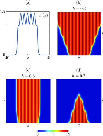
Fig. 1: Time simulations of the PDE model (7) with synaptic kernel (2) and sigmoidal firing rate (4), posed on a large domain $x\in[-L_{x},L_{x}]$ with Neumann boundary conditions $\partial_{x}u(\pm L_{x},t)=0$. Panel (a): initial condition used in the simulations. Panel (b): the periodic core invades the domain (time runs upwards) as two pulsating fronts travel towards the boundary. Panel (c): a stable localized steady state is formed. Panel (d): the homogeneous background invades the domain. Parameters: $L_{x}=90$ (plots show an inset $(x,t)\in[-40,40]\times[0,50]$), $\nu=50$, $a=0.3$, $\epsilon=1$. Spatial operators are discretized via finite differences with $3000$ gridpoints.

When $f$ is a smooth sigmoid, it is advantageous to reformulate the nonlocal problem (1) as a local PDE, more suitable for direct numerical simulation and numerical continuation. Following [40, 20, 16, 18, 39], we take the Fourier transform of (1), with kernel expressed by (2)

$$\partial_{t}\hat{u}(\xi,t)=-\hat{u}(\xi,t)+\hat{w}(\xi)\widehat{\big{(}Af(u)\big{)}}(\xi,t),$$

where $\hat{w}(\xi)=(2\pi)^{-1}/(\xi^{2}+1)$. Multiplying the previous equation by $\xi^{2}+1$ and taking the inverse Fourier transform we obtain

$$(1-\partial^{2}_{x})(\partial_{t}u+u)=A(x)f(u),$$ (7)

where the dependence of $u$ on $x$ and $t$ has been omitted for simplicity. Once complemented with suitable initial and boundary conditions, the equation above constitutes an equivalent PDE formulation of the model problem. Steady states are solutions to

$$0=(\partial^{2}_{x}-1)q+A(x)f(q)$$ (8)

and linear stability is inferred via the generalized eigenvalue problem

$$(1+\lambda)(1-\partial^{2}_{x})v=A(x)f^{\prime}(q)v.$$ (9)

In passing we note that time simulations of (7) and stability calculations (9) can be carried out numerically without forming a discretization for $(1-\partial^{2}_{x})^{-1}$ (see [18]). In Figure 1 we show time simulations of (7) posed on the interval $[-90,90]$ with Neumann boundary conditions, for various values of the firing rate threshold $h$. For selected values of $h$, we find stable localized solutions, which destabilize as the parameter is increased or decreased. Time-dependent solutions, such as the ones shown in Figures 1(b) and 1(d), have been previously analyzed by Coombes and Laing [16], whereas in the present paper we focus on the existence and bifurcation structure of stationary localized states.

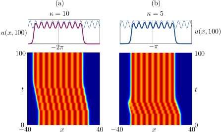
Fig. 2: Time simulations of the PDE model (7) with instantaneous phase slips in the kernel modulation (10). Panel (a): with $\kappa=10$ we obtain a localized steady state that is symmetric with respect to the axis $x=-2\pi$. Panel (b): for $\kappa=5$, the steady state is symmetric with respect to the axis $x=-\pi$. Parameters as in Figure 1(c). In the top panels we plot reference curves that are spatially in phase with the inhomogeneity $A$.

The simulations in Figure 1 are compatible with a snakes-and-ladders bifurcation structure and, owing to the spatial modulation, we expect to find stable localized states that are spatially in-phase with $A$ and centered around its local minima and maxima. In Figure 2 we fix $h$ and perturb a localized steady state with abrupt phase slips in the kernel modulation. More precisely we set

$$A(x,t)=1+a\cos\bigg{(}\frac{x}{\varepsilon}+\sum_{i=1}^{4}i\frac{\pi}{2}\chi_{[t_{i},t_{i+1}]}(t)\bigg{)}$$ (10)

where $t_{i}=10+i\kappa$ and $\chi_{[t_{i},t_{i+1}]}$ is the indicator function with support $[t_{i},t_{i+1}]$. After four phase slips, we return to the original spatial inhomogeneity $A(x)=1+a\cos(x/\varepsilon)$, which is kept constant thereafter. Perturbations with $\kappa=10$ elicit a localized steady state that is symmetric with respect to the axis $x=-2\pi$, whereas shorter phase slips, with $\kappa=5$, give rise to states that are symmetric with respect to the axis $x=-\pi$.

In local models supporting localized states, symmetries of the PDE are reflected in the bifurcation structure: each snaking branch includes solutions with the same symmetry and intertwined branches are connected by ladders of asymmetric solutions. In one-dimensional snaking systems with spatial reversibility, localized states can be interpreted from a spatial-dynamical systems viewpoint and symmetries of the PDE correspond to reversers of the spatial-dynamical system [5, 45]. Following this approach, we recast (8) as a first-order non-autonomous system in $x$

$$\frac{\mathop{}\!\mathrm{d}}{\mathop{}\!\mathrm{d}x}\begin{pmatrix}U_{1}\\ U_{2}\end{pmatrix}=\begin{pmatrix}U_{2}\\ U_{1}-A(x)f(U_{1})\end{pmatrix},$$ (11)

where we posed $(U_{1},U_{2})=(q,q_{x})$. Localized steady states of the nonlocal model correspond to bounded solutions to (11) that decay exponentially as $|x|\to\infty$. System (11) is reversible: for each $n\in\mathbb{Z}$, we consider the following autonomous extension

$$\frac{\mathop{}\!\mathrm{d}}{\mathop{}\!\mathrm{d}x}\begin{pmatrix}U_{1}\\ U_{2}\\ U_{3}\end{pmatrix}=\begin{pmatrix}U_{2}\\ U_{1}-A(U_{3}+n\pi\varepsilon)f(U_{1})\\ 1\end{pmatrix},\qquad n\in\mathbb{Z}$$

with reverser

$$\mathcal{R}\colon(U_{1},U_{2},U_{3})\mapsto(U_{1},-U_{2},-U_{3}).$$

Conversely, we say that a solution is asymmetric if $\mathcal{R}q\neq q$. The stationary profiles plotted in Figures 2(a) and 2(b) correspond to an even- and odd-symmetric solution, respectively.

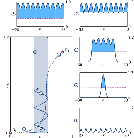
Fig. 3: Branches of periodic and localized steady states of the integral model with inhomogeneous kernel (2) with $a=0.3$, $\varepsilon=1$ and Heaviside firing rate. The bifurcation diagram is plotted in terms of the norm $\|u\|^{2}_{2}=1/(2L_{x})\int_{-L_{x}}^{L_{x}}|u(x)|^{2}\,dx$, where $L_{x}=\pi\varepsilon$ for periodic solutions and $L_{x}=30$ for localized solutions. The trivial steady state $u(x)\equiv 0$ coexists with the fully periodic state for $h\in\big{(}0,1-a\varepsilon^{2}/(1+\varepsilon^{2})\big{)}$. A snaking branch of even-symmetric localized solutions emanates from $B_{0}$. As we ascend the snaking diagram, more bumps are formed. Example solutions are plotted in the panels. For reference, we also plot the activity threshold $u(x)\equiv h$ (dashed magenta). There exist (not shown) a snaking branch of localized odd-symmetric solutions, as well as ladder branches connecting the two snaking branches.

The spatial-dynamic formulation developed in [5, 45] for the Swift–Hohenberg equation allows predictions of snaking branches of localized patterns from the bifurcation structure of fronts connecting the trivial (background) state to the core state.

We can not directly apply this theory to our case, in that system (11) is non-autonomous, and $(0,0)$ is not an equilibrium . However, we shall see that the in the limit of Heaviside firing rate, which gives rise to a non-smooth spatial-dynamic formulation, we are able to compute explicit expressions for connecting orbits and, hence, for the snaking bifurcation diagram, which we partially present in Figure 3. For sigmoidal firing rates we will adopt numerical continuation and compute snaking bifurcation branches solving the boundary-value problem (8) and the associated stability problem (9).

4 Steady states for Heaviside firing rate

In the case of Heaviside firing rate, localized steady states with two threshold crossings can be constructed explicitly for the inhomogeneous model and their stability can be inferred solving a simple 2-by-2 eigenvalue problem. To each steady state $q$ with firing threshold $h$, we associate an active region $\mathcal{B}=\Set{x\in\mathbb{R}}{q(x)>h}$, that is, a subset of the real line in which $q$ is above threshold. In the case of Heaviside firing rate, this implies that $H(q(x))\equiv 1$ if $x\in\mathcal{B}$ and $0$ otherwise. Equation (5) can be rewritten as

$$q(x)=\int_{x_{1}}^{x_{2}}w(|x-y|)A(y)\mathop{}\!\mathrm{d}{y}.$$ (12)

If the threshold crossings $x_{1,2}$ are known, then (12) yields the profile of the stationary solution. The boundaries $x_{1}$ and $x_{2}$ can be determined as functions of system parameters by enforcing the threshold crossing conditions $q(x_{1})=h$, $q(x_{2})=h$.

If $f$ is the Heaviside function, the nonlocal eigenvalue problem (6) is written as

In the following sections we will apply this framework to both periodic and localized solutions in the Heaviside limit.

Remark 1 (Number of threshold crossings).

The framework presented here can be extended to patterns with an arbitrary number of threshold crossings; however, throughout this paper we will restrict analytic calculations to solutions that have only two threshold crossings, or to spatially-periodic patterns with two threshold crossings per period. The linear stability analysis outlined here is valid for small perturbations $v$ that have the same number of threshold crossings of $q$.

Remark 2 (Stability of solutions with no threshold crossing).

Solutions that do not cross threshold are linearly stable, in that the eigenvalue problem (13) gives a single eigenvalue $\lambda=-1$.

5 Homogeneous and spatially periodic solutions for Heaviside firing rates

We now begin exploring steady state solutions to the integral model (1) with inhomogeneous kernel (2) and Heaviside firing rate $f(u)=H(u-h)$. If the kernel is homogeneous, a straightforward computation shows that localized solutions exist and are linearly unstable. These patterns are organized in parameter space with a non-snaking bifurcation diagram: we integrate (12) with $a=0$, $x_{1,2}=\pm L/2$ and obtain

$$q(x)=\begin{cases}1-{\rm e}^{-L/2}\cosh x&\text{if $|x|<L/2$,}\\ {\rm e}^{-|x|}\sinh(L/2)&\text{otherwise}\end{cases}$$

where $h=(1-{\rm e}^{-L})/2$. Using (16) we find $\lambda_{1,2}\geq 0$. We plot these solutions and their bifurcation diagram in Figure 4.

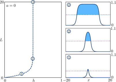
Fig. 4: Bifurcation diagram for localized fronts for the homogeneous kernel. Left: branch of localized unstable fronts obtained for $a=0$. We use the width $L$ of the active region as a solution measure. The branch does not snake and approaches a vertical asymptote. Right: selected profiles along the branch.

From now on, we will concentrate on the more interesting case $a>0$.

Owing to the inhomogeneity, the only spatially-homogeneous solution is the trivial state $q_{0}(x)\equiv 0$: posing $q(x)\equiv\kappa$ we obtain

$$\kappa=H(\kappa-h)\int_{-\infty}^{\infty}W(x,y)\mathop{}\!\mathrm{d}y,\qquad$$

from which we deduce $0=\kappa<h$. The trivial solution is linearly stable for strictly positive $h$ (see Remark 2).

Spatially-periodic states are also supported by the integral model. In A we show that $2\pi\varepsilon$-periodic solutions satisfy

$$q(x)=\int_{-\pi\varepsilon}^{\pi\varepsilon}\tilde{w}(|x-y|)A(y)f(q(y))\mathop{}\!\mathrm{d}y,\qquad x\in[-\pi\varepsilon,\pi\varepsilon)$$ (17)

$$q(-\pi\varepsilon)=q(\pi\varepsilon),$$ (18)

where

$$\widetilde{w}(x)=\frac{1}{2}{\rm e}^{-x}+\frac{{\rm e}^{-2\pi\varepsilon}}{1-{\rm e}^{-2\pi\varepsilon}}\cosh\left(x\right).$$ (19)

In other words, if we seek a stationary $2\pi\varepsilon$-periodic solution, then we may pass from an integral equation posed on $\mathbb{R}$ to a reduced integral formulation posed on the interval $[-\pi\varepsilon,\pi\varepsilon]$, provided that we use the amended kernel $\widetilde{w}$ instead of $w$. In passing, we note that similar conditions for periodic solutions can be derived for generic exponential kernels.

We now specialize the problem (17)–(19) to the case of Heaviside firing rate $f(u)=H(u-h)$, construct $2\pi\varepsilon$-periodic stationary solutions and explore their bifurcation structure. The simplest type of stationary periodic state of the model is the above-threshold solution $q_{\textrm{at}}$, that is, a solution that lies above threshold $h$ for all $x\in\mathbb{R}$. We then formulate the following problem:

Problem 3 (Above-threshold periodic solutions).

For fixed $h,a,\varepsilon\in\mathbb{R}^{+}$, find a smooth $2\pi\varepsilon$-periodic function $q_{\textrm{at}}$ such that

$$\begin{split}q_{\textrm{at}}(x)&=\int_{-\pi\varepsilon}^{\pi\varepsilon}\widetilde{w}(|x-y|)A(y)\mathop{}\!\mathrm{d}y,\qquad x\in[-\pi\varepsilon,\pi\varepsilon),\\ h&<\min_{x\in[-\pi\varepsilon,\pi\varepsilon)}q_{\textrm{at}}(x),\end{split}$$

An explicit solution $q_{\textrm{at}}$ can be computed in closed form for the specific kernel (19), yielding

$$q_{\textrm{at}}(x)=1+\frac{a\varepsilon^{2}}{1+\varepsilon^{2}}\cos\frac{x}{\varepsilon},\quad x\in[-\pi\varepsilon,\pi\varepsilon),$$ (20)

for $h\in\big{(}0,1-a\varepsilon^{2}/(1+\varepsilon^{2})\big{)}$. Since there are no threshold crossings, $q_{\textrm{at}}$ is stable in this interval of $h$ for all values of $a$ and $\varepsilon$. In Figure 3, we show an example of $q_{\textrm{at}}$ for $a=0.3$, $\varepsilon=1$ (solution label $5$).

We now turn to the more interesting case of periodic solutions that cross threshold. The simplest of such cross-threshold states, $q_{\textrm{ct}}$, are solutions that attain the value $h$ exactly twice in $[-\pi\varepsilon,\pi\varepsilon)$, as shown in Figure 5(a). More precisely, we derive cross-threshold solutions as follows:

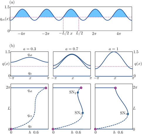
Fig. 5: Periodic solutions in the Heaviside limit. (a) Construction of an even periodic solution $q_{\textrm{ct}}$ with exactly $2$ threshold crossings in each period. (b) Branches of periodic solutions for $\varepsilon=1$ and various values of $a$. A branch of unstable solutions $q_{\textrm{ct}}$ connects the branch of trivial steady states $q_{0}$ to the branch of above-threshold periodic solutions $q_{\textrm{at}}$ (bottom left); for suitable combinations of $a$ and $h$ the system admits three stable solutions (bottom center). A further increase of $a$ leads to a new bistable regime. Stable solutions at $h=0.6$ are shown in the top panels.

Problem 4 (Cross-threshold periodic solutions).

For fixed $h,a,\varepsilon\in\mathbb{R}^{+}$, find an even $2\pi\varepsilon$-periodic smooth function $q_{\textrm{ct}}$ and a number $L\in(0,2\pi\varepsilon)$ such that

$$q_{\textrm{ct}}(L/2)=h,$$ (21)

$$q_{\textrm{ct}}(x)=\int_{-L/2}^{L/2}\widetilde{w}(|x-y|)A(y)\,\mathop{}\!\mathrm{d}y,\qquad\text{for $x\in[-\pi\varepsilon,\pi\varepsilon)$}.$$ (22)

The first equation implies that the threshold crossing occurs at points $x=\pm L/2$, whereas the second one is simply derived from Equation (17) using the identity $f(q_{\textrm{ct}}(x))\equiv 1$ for $x\in[-L/2,L/2]$.

Remark 5 (Bifurcation equation for periodic solutions).

Inspecting Problem 4 we notice that the width $L$ of the active region of $q_{\textrm{ct}}$ is a function of the threshold crossing $h$: combining (21) and (22) we obtain

$$h=I_{\textrm{ct}}(L):=\int_{-L/2}^{L/2}\widetilde{w}(|L/2-y|)A(y)\,\mathop{}\!\mathrm{d}y.$$ (23)

In analogy with [5], we call the equation above a bifurcation equation for periodic solutions $q_{\textrm{ct}}$. Explicit formulae for the solution profile $q_{\textrm{ct}}$ and the corresponding bifurcation equation are given in B.

The stability of a stationary profile $(q_{\textrm{ct}},L)$ is found in a similar fashion to what was done for stationary states in Section 4, with the original kernel $w$ replaced by the amended kernel $\tilde{w}$. We find

$$\begin{split}(1+\lambda)v(x)&=\int_{-\pi\varepsilon}^{\pi\varepsilon}\widetilde{w}(|x-y|)A(y)\sum_{i=1}^{2}\frac{\delta(q_{\textrm{ct}}(y)-x_{i})}{|q_{\textrm{ct}}^{\prime}(y)|}v(y)\,\mathop{}\!\mathrm{d}y\end{split}$$ (24)

where $x_{1,2}=\mp L/2$. Evaluating the equation above at $x=x_{1,2}$ yields the pair of eigenvalues

$$\lambda_{1,2}=-1+(\tilde{w}(0)\pm\tilde{w}(L))\frac{A(x_{0}+L/2)}{|q_{\textrm{ct}}^{\prime}(x_{0}+L/2)|},$$

where we have made use of the fact that $|q_{\textrm{ct}}^{\prime}(x)|$ and $A(x)$ are even. We are now ready to study the bifurcation structure of periodic solutions in greater detail.

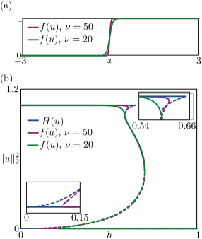
Fig. 6: Branches of periodic solutions for Heaviside firing rate and steep sigmoidal firing rates. Panel (a): sigmoidal firing rates (4) with $h=0$ and $\nu=20,50$. Panel (b): bifurcation diagram of the integral model for $a=0.7$ and $\varepsilon=1$; in the Heaviside limit a branch of periodic solutions connects the trivial steady state $q_{0}$ to the above-threshold periodic state $q_{\textrm{at}}$; for sigmoidal firing rates the trivial steady state does not exist, but the branch behaves in a similar fashion, with $2$ saddle-nodes on the branch for $\nu=20$ and $4$ saddle-nodes on the branch for $\nu=50$.

In the Heaviside limit we use Equations (21)–(24) which allow us to compute the solution profile, its activity region $L$ and its stability as a function of $h$. The resulting bifurcation diagrams are shown in Figure 5(b). The main continuation parameter is $h$ and we set $\varepsilon=1$, $a\in\{0.3,0.7,1\}$: for small values of $a$ the trivial state $q_{0}$ coexists with the above threshold solution $q_{\textrm{at}}$ for $0<h<\big{(}0,1-a\varepsilon^{2}/(1+\varepsilon^{2})\big{)}$. At the grazing point $h=1-a\varepsilon^{2}/(1+\varepsilon^{2})$, the above threshold solution becomes tangent to $u(x)\equiv h$.

The branches of $q_{0}$ and $q_{\textrm{at}}$ are connected by a branch of cross-threshold solutions which are initially unstable. As we increase $a$, two saddle node bifurcations emerge on the cross-threshold branch, at a cusp, and there exists an interval of $h$ in which $q_{0}$, $q_{\textrm{ct}}$ and $q_{\textrm{at}}$ coexist and are stable. As $a$ is further increased, only one saddle node persists and we have an extended bistability region. We refer the reader to Section 7 for a more detailed study of the two-parameter bifurcation diagram.

We can also study the case of continuous sigmoidal firing rates (4) using standard numerical bifurcation analysis techniques: we find steady states $q$ solving (8) with Neumann boundary conditions and we continue the solution in parameter space with pseudo-arclength continuation [29] using the secant code developed in [51]. A comparison between bifurcation diagrams for Heaviside and sigmoidal firing rates is presented in Figure 6. The solution branches are in good agreement, with the exception of the fold points, as it can be seen in the insets.

6 Construction and bifurcation structure of localized solutions for Heaviside firing rates

Localized steady states are solutions to (1) which decay to zero as $|x|\to\infty$ and for which the activity region $\mathcal{B}$ is a finite disjoint union of bounded intervals [2, 25]. In Figure 1 we have shown time simulations of the PDE model (7) posed on a large finite domain with Neumann boundary conditions and steep sigmoidal firing rate with $\nu=50$. The parameters are chosen such that the trivial solution $q_{0}$ and the above-threshold periodic solution $q_{\textrm{at}}$ are supported in the Heaviside firing rate case. As expected, stable localized patterns are found in this region.

In this section, we construct such patterns analytically and study their stability. As it was done in Section 5, we will perform analytical or semi-analytical calculations in the Heaviside limit, whereas we will employ numerical continuation for sigmoidal firing rates.

As seen in Section 4, a generic bump $q_{\textrm{b}}$ with active region $\mathcal{B}=(x_{1},x_{2})\subset\mathbb{R}$ satisfies, in the Heaviside limit,

$$q_{\textrm{b}}(x)=\int_{x_{1}}^{x_{2}}w(|x-y|)A(y)\mathop{}\!\mathrm{d}y.$$ (25)

Without loss of generality, we pose $x_{1,2}=x_{0}\mp L/2$. We note that if $L=0$ then $q_{\textrm{b}}$ coincides with the trivial solution. In analogy with the periodic case, we find a localized solution as follows:

Problem 6 (Localized solutions).

For fixed $h,a,\epsilon\in\mathbb{R}^{+}$ find a smooth function $q_{\textrm{b}}$ and scalars $x_{0}\in\mathbb{R}$, $L\in\mathbb{R}^{+}$, such that

$$q_{\textrm{b}}(x_{0}-L/2)=h,$$ (26)

$$q_{\textrm{b}}(x_{0}+L/2)=h,$$ (27)

$$q_{\textrm{b}}(x)=\int_{x_{0}-L/2}^{x_{0}+L/2}w(|x-y|)A(y)\,\mathop{}\!\mathrm{d}y,\qquad x\in\mathbb{R}.$$ (28)

Remark 7.

In the problem above we do not enforce explicitly asymptotic conditions for $q_{\textrm{b}}$, since they are implied by (28) for our particular choice of $w$ and $A$. Indeed, let $A_{\ast}=\max_{x\in\mathbb{R}}|A(x)|$, then

$$0\leq|q_{\textrm{b}}(x)|\leq A_{\ast}\int_{x_{0}-L/2}^{x_{0}+L/2}w(|x-y|)\,\mathop{}\!\mathrm{d}y,$$

hence $|q_{\textrm{b}}(x)|\to 0$ as $|x|\to\infty$.

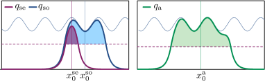
Fig. 7: Examples of localized stationary solutions constructed in the Heaviside limit (dashed magenta line indicates the firing threshold $h$). Left: symmetric solutions satisfy $q(x-x_{0})=q(x_{0}-x)$ where $x_{0}=n\pi\varepsilon$, $n\in\mathbb{Z}$. Even- (Odd-) symmetric solutions, $q_{\textrm{se}}$ ($q_{\textrm{so}}$), are characterized by $n$ even (odd). The profiles in the pictures are constructed for $h=0.55$, $a=0.3$, $\varepsilon=1$. As expected, peaks of localized solutions are in phase with peaks of the periodic solution $q_{\textrm{at}}$. Right: localized asymmetric solutions satisfy $\Psi_{\textrm{asym}}(L;\varepsilon)=0$ (see Equation (31)); for these patterns $x_{0}$ varies in a continuous interval. The asymmetric solution is constructed for $h=0.5$, $a=0.3$, $\varepsilon=1$.

In Section 3 we discussed symmetric and asymmetric solutions in the context of spatial-dynamical systems of the PDE associated with the integral model. Equivalently, a solution is symmetric if $q_{\textrm{b}}(x-x_{0})=q_{\textrm{b}}(x_{0}-x)$ and asymmetric otherwise. Problem 6 does not provide a direct way to distinguish between symmetric and asymmetric states, but it can be reformulated so as to avoid this limitation. Each solution $(q_{\textrm{b}},x_{0},L)$ to Problem 6 is such that $q_{\textrm{b}}(x_{0}-L/2)=q_{\textrm{b}}(x_{0}+L/2)$, which can be written as

$$\Psi_{\textrm{sym}}(x_{0})\Psi_{\textrm{asym}}(L)=0,$$ (29)

where

$$\Psi_{\textrm{sym}}(x_{0})=\sin\bigg{(}\frac{x_{0}}{\varepsilon}\bigg{)},$$ (30)

$$\Psi_{\textrm{asym}}(L)=(1-{\rm e}^{-L})\cos\bigg{(}\frac{L}{2\varepsilon}\bigg{)}-(1+{\rm e}^{-L})\varepsilon\sin\bigg{(}\frac{L}{2\varepsilon}\bigg{)}.$$ (31)

Crucially, (29) holds if either $\Psi_{\textrm{sym}}=0$ or $\Psi_{\textrm{asym}}=0$, so we are now ready to construct symmetric and asymmetric localized solutions as follows:

Problem 8 (Symmetric and asymmetric localized solutions).

For fixed $h,a,\epsilon\in\mathbb{R}^{+}$, find a smooth nonnegative function $q_{\textrm{b}}$ and scalars $x_{0}\in\mathbb{R}$, $L\in\mathbb{R}^{+}$, such that

$$\Psi_{\textrm{sym}}(x_{0})=0,\qquad\text{(or $\Psi_{\textrm{asym}}(L)=0$)}$$ (32)

$$q_{\textrm{b}}(x_{0}+L/2)=h,$$ (33)

$$q_{\textrm{b}}(x)=\int_{x_{0}-L/2}^{x_{0}+L/2}w(|x-y|)A(y)\,\mathop{}\!\mathrm{d}y,\qquad x\in\mathbb{R}.$$ (34)

In symmetric states, the symmetry condition (30) fixes the value of $x_{0}$; more precisely we have $x_{0}=n\pi\varepsilon$ for $n\in\mathbb{Z}$, therefore we distinguish between even- and odd-symmetric solutions, depending on the value of $n$. On the other hand, in asymmetric states the width $L$ is fixed by the asymmetry condition (31) and $x_{0}$ is not restricted to assume discrete values.

For our choice of the connectivity function $w$ and modulation $A$ we derive closed-form expressions for symmetric and asymmetric localized states.

For the profile of symmetric solutions we find

$$q_{\textrm{b}}(x)=\begin{cases}\displaystyle{1+\frac{a\epsilon^{2}}{1+\epsilon^{2}}\cos\frac{x}{\epsilon}-\Theta_{1}(L;x_{0})\cosh\left(x_{0}-x\right)}&\text{if $|x-x_{0}|<L/2$,}\\ \displaystyle{\Theta_{2}(L;x_{0})\,\exp{(-|x-x_{0}|+L/2)}}&\text{otherwise,}\end{cases}$$ (35)

where the auxiliary functions $\Theta_{1}$ and $\Theta_{2}$ are given by

$$\Theta_{1}(L;x_{0})=\left[1+\frac{a\epsilon}{\sqrt{1+\epsilon^{2}}}\cos\frac{x_{0}}{\epsilon}\cos\left(\frac{L}{2\epsilon}+\Phi\right)\right]{\rm e}^{-L/2},$$

$$\begin{split}\Theta_{2}(L;x_{0})=&\frac{1-{\rm e}^{-L}}{2}+\frac{a}{2}\frac{\varepsilon}{\sqrt{\varepsilon^{2}+1}}\cos\frac{x_{0}}{\varepsilon}\\ &\times\left[\cos\left(\frac{L}{2\varepsilon}-\Phi\right)-{\rm e}^{-L}\cos\left(\frac{L}{2\varepsilon}+\Phi\right)\right].\end{split}$$

In the above expressions we posed $\Phi=\arctan\epsilon^{-1}$ and we exploited the fact that $\sin(x_{0}/\epsilon)=0$.

Similarly, for asymmetric solutions we obtain

$$q_{\textrm{b}}(x)=\begin{cases}\displaystyle{1+\frac{a\epsilon^{2}}{1+\epsilon^{2}}\cos\frac{x}{\epsilon}-\Lambda_{1}(x,x_{0};L)}&\text{if $|x-x_{0}|<L/2$,}\\ \displaystyle{\Lambda_{2}(x_{0};L)\,\exp(-|x-x_{0}|+L/2)}&\text{otherwise,}\end{cases}$$

with auxiliary functions $\Lambda_{1}$ and $\Lambda_{2}$ given by

$$\begin{split}\Lambda_{1}(x,x_{0};L)=\frac{a\epsilon}{\sqrt{1+\epsilon^{2}}}{\rm e}^{-L/2}\bigg{\{}\sinh(x_{0}-x)\sin\frac{x}{\epsilon}\sin\left(\frac{L}{2\epsilon}+\Phi\right)\\ +\cosh(x_{0}-x)\cos\frac{x}{\epsilon}\cos\left(\frac{L}{2\epsilon}+\Phi\right)\bigg{\}},\end{split}$$

$$\Lambda_{2}(x_{0};L)=\frac{1-{\rm e}^{-L}}{2}\bigg{[}1+a\cos\bigg{(}\frac{x_{0}}{\varepsilon}\bigg{)}\cos\bigg{(}\frac{L}{2\varepsilon}\bigg{)}\bigg{]}.$$

Examples of symmetric and asymmetric localized solutions are plotted in Figure 7. These patterns are computed in a region of parameter space where the trivial solution $q_{0}$ and the periodic above-threshold $q_{\textrm{at}}$ solution coexist. As expected, localized solutions are in-phase with the inhomogeneity $A$.

Remark 9 (Bifurcation equation for localized solutions).

Similarly to the periodic case, $h$ is related to $L$ and $x_{0}$ via a bifurcation equation. For a solution $(q_{\textrm{b}},x_{0},L)$ of Problem 8, we find the general expression

$$h=I_{\textrm{b}}(L,x_{0}):=\int_{x_{0}-L/2}^{x_{0}+L/2}w(|x_{0}+L/2-y|)A(y)\,\mathop{}\!\mathrm{d}y.$$

which can be specialized for the symmetric and asymmetric cases as follows:

$$h=I_{\textrm{sym}}(L;x_{0}):= \Theta_{2}(L;x_{0})$$ (36)

$$h=I_{\textrm{asym}}(x_{0};L):= \Lambda_{2}(x_{0};L),$$ (37)

where $\Theta_{2}$ and $\Lambda_{2}$ are auxiliary functions defined above. In the bifurcation function $I_{\textrm{sym}}$ the value of $x_{0}$ is fixed by the condition $\Psi_{\textrm{sym}}(x_{0})=0$, hence $\cos(x_{0}/\epsilon)=\pm 1$. Similarly, $L$ is fixed in the expression of $I_{\textrm{asym}}$ and its value is determined by $\Psi_{\textrm{asym}}(L)=0$.

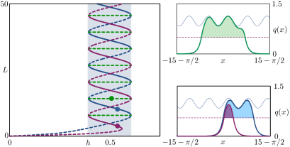
Fig. 8: Snakes and ladders computed in the Heaviside limit. Selected profiles along the branch are reported on the right (they correspond to the ones in Figure 7). Parameters as in Figure 7.

Following [5], we notice that the bifurcation equation (36) is a parametrization of snaking branches of even- and odd-symmetric solutions, whereas equation (37) is a parametrization of ladder branches of asymmetric solutions: indeed both $x_{0}$ and $L$ depend on $h$, as they solve Problem 8. In this case, however, the bifurcation equations are available in closed form so we can proceed directly to plot snakes and ladders. In Figure 8, we fix $a$ and $\varepsilon$, construct localized solutions and plot their bifurcation diagrams as loci of points on the $(L,h)$-plane that satisfy the bifurcation equations. In particular we use $I_{\textrm{sym}}(L;0)$ and $I_{\textrm{sym}}(L;\pi\varepsilon)$ to plot representative branches of even- and odd-symmetric solutions, respectively. As expected, in the limit for large $L$, $I_{\textrm{sym}}$ is well approximated by a cosinusoidal function. On the other hand, ladders are found using $I_{\textrm{asym}}(x_{0};L)$, where $L$ satisfies the asymmetry condition $\Psi_{\textrm{asym}}(L)=0$.

The stability problem of a localized state $(q_{\textrm{b}},x_{0},L)$ is determined following the scheme outlined in Section 2: we use , with threshold crossings $x_{1,2}=x_{0}\mp L/2$. For symmetric solutions we find

$$\lambda_{1,2}=-1+(w(0)\pm w(L))\frac{A(x_{0}+L/2)}{|q_{\textrm{b}}^{\prime}(x_{0}+L/2)|}.$$ (38)

In Figure 9 we plot eigenvalues $\lambda_{1,2}$, along the even-symmetric snaking branch for $n=0$. The results show that solutions on this branch undergo a sequence of saddle-nodes and pitchfork bifurcations, as indicated by the corresponding eigenfunctions. Similar results (not shown) are found for odd-symmetric states.

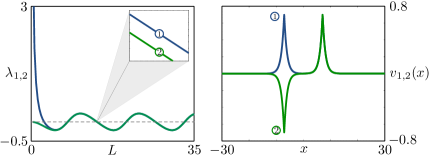
Fig. 9: Eigenvalues and eigenfunctions of localized even-symmetic solutions. Left: eigenvalues of localized even-symmetric solutions along the snaking branch of Figure 8 (see Equation (38)). Right: eigenfunctions of selected states, in the proximity of a saddle node and a pitchfork on the snaking branch.

For asymmetric solutions we obtain

$$\lambda_{1,2}=\frac{{\rm e}^{-L}}{1-{\rm e}^{-L}}\pm\frac{\Gamma(L)}{2|q_{\textrm{b}}^{\prime}(x_{0}+L/2)|},$$ (39)

where

$$\Gamma(L)=\sqrt{\left(1+{\rm e}^{-2L}\right)\left(a\sin\frac{x_{0}}{\varepsilon}\sin\frac{L}{2\varepsilon}\right)^{2}+{\rm e}^{-2L}\left(1+a\cos\frac{x_{0}}{\varepsilon}\cos\frac{L}{2\varepsilon}\right)^{2}}.$$ (40)

Here we have made use of the fact that, with our choice of the synaptic kernel, we have

$$|q_{\textrm{b}}^{\prime}(x_{0}-L/2)|=|q_{\textrm{b}}^{\prime}(x_{0}+L/2)|=I_{\textrm{asym}}(x_{0};L),$$ (41)

which is found by differentiating (6). Further, we note that

$$\Gamma(L)\geq{\rm e}^{-L}\left(1+a\cos\frac{x_{0}}{\varepsilon}\cos\frac{L}{2\varepsilon}\right).$$ (42)

By using (37), (41) and (42) we see that the eigenvalues $\lambda_{1,2}$ are such that $\lambda_{1}>0$ and $\lambda_{2}\leq 0$. As a consequence, all asymmetric solutions are linearly unstable. For completeness, we find values of $h$ at which pitchfork bifurcations are attained: such points can also be computed analytically by setting $I_{\textrm{sym}}=I_{\textrm{asym}}$ and obtaining

$$h=\frac{1-{\rm e}^{-L}}{2}\left(1+a\cos\frac{x_{0}}{\epsilon}\cos\frac{L}{2\epsilon}\right),\quad\cos(x_{0}/\epsilon)=\pm 1$$

at which

$$\lambda_{1}=\frac{2{\rm e}^{-L}}{1-{\rm e}^{-L}},\qquad\lambda_{2}=0.$$ (43)

The snake-and-ladder bifurcation structure derived here for Heaviside firing rates is also found in the case of steep sigmoidal firing rates: in particular, we have performed numerical continuation for the firing rate function (4) with $\nu=50$ and found an analogous bifurcation diagram (not shown).

7 Changes in the modulation amplitude

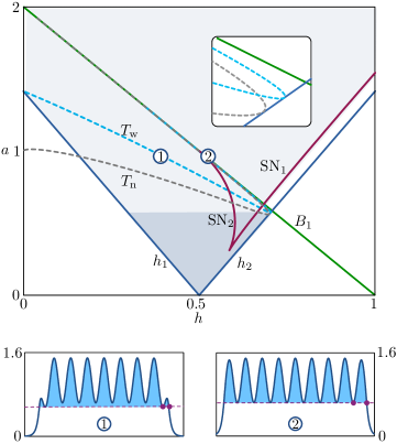
Fig. 10: Two-parameter bifurcation diagram for Heaviside firing rates in the $(a,\varepsilon)$-plane. Top: We plot the grazing curve $B_{1}$ (in green), below which we have bistability between $q_{0}$ and $q_{\textrm{at}}$, curves of snaking limits $h_{1,2}$ (blue), curves of saddle nodes bifurcations of $q_{\textrm{ct}}$, $\textrm{SN}_{1,2}$ (magenta) and lines at which a simple threshold crossing is followed by a tangency in wide ($T_{\textrm{w}}$, dashed blue line, ) and narrow ($T_{\textrm{n}}$, dashed grey line) solutions. We find a simple snake and ladder scenario in the shaded blue area and a more complicated snaking scenario in the shaded grey area. Bottom: selected solution profiles on the curve $T_{\textrm{w}}$.

The framework developed in the previous Sections can be employed to study two-parameter bifurcation diagrams. So far, we have fixed the parameters $a$, $\varepsilon$ and used $h$ as our main continuation parameter. It is interesting to explore how variations in secondary parameters affect the snaking branches. In [35], the authors explore variations in the spatial scale of the heterogeneity for the Swift–Hohenberg equation. Here, we concentrate on the amplitude $a$ of the heterogeneity $A(x)$ for the integral neural field model. Following the previous sections, we study the Heaviside case analytically and then present numerical simulations for the steep sigmoid case.

We begin by considering Heaviside firing rate and outlining the region of parameter space where the trivial steady state $q_{0}$ and the above-threshold periodic solution $q_{\textrm{at}}$ coexist and are stable, that is, we follow the grazing point $B_{1}$ in Figure 3 in the $(a,h)$ plane. The curve is found by imposing the tangency condition $h=\min_{x\in[-\pi\varepsilon,\pi\varepsilon)}q_{\textrm{at}}(x)$, which combined with Equation 20 gives the locus of points

$$a=(1-h)\frac{1+\varepsilon^{2}}{\varepsilon^{2}},\qquad h\in(0,1),$$ (44)

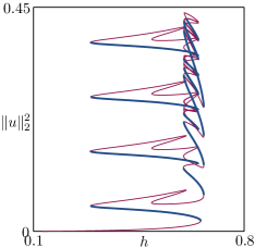
Fig. 11: Branch of even solutions for sigmoidal firing rate with $a=0.6$, $\nu=50$, $\varepsilon=1$. Stable (Unstable) branches are indicated with thick blue (thin magenta) lines.

In Figure 10 we present a two-parameter bifurcation diagram and indicate with a green line the locus of grazing points (44): $q_{\textrm{at}}$ and $q_{0}$ coexist and are stable if $(a,h)$ is below the green line. Next, we compute the snaking limits, for large $L$, as functions of $h$ and $a$. We use the bifurcation equation for symmetric localized states, Equation (36), and find in the limit for large $L$ the following snaking limits

$$h_{1,2}=\frac{1}{2}\bigg{(}1\pm\frac{a\varepsilon}{\sqrt{1+\varepsilon^{2}}}\bigg{)}$$

These curves are plotted in Figure 10 (solid blue lines). Further, we compute the loci of saddle-node bifurcations of the cross-threshold solutions $q_{\textrm{ct}}$ (which are labeled $SN_{1}$ and $SN_{2}$ in Figure 5) by solving for $(a,h)$ the following system

$$h-I_{\textrm{ct}}(L;x_{0})=0$$

$$\frac{\mathop{}\!\mathrm{d}}{\mathop{}\!\mathrm{d}L}I_{\textrm{ct}}(L;x_{0})=0$$

The loci of saddle-node bifurcations are plotted with dark magenta lines in Figure 10. The area between these two curves identifies a region in which $q_{\textrm{ct}}$, $q_{\textrm{at}}$ and $q_{0}$ coexist and are stable. In passing we note that the curve for $SN_{2}$ intersects the curve for the grazing point $B_{1}$ at $a=1$.

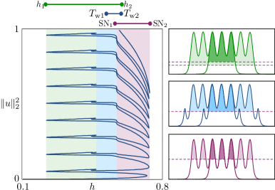
Fig. 12: Bifurcation diagram for $a=0.8$ $\nu=50$, $\varepsilon=1$. The snaking branch is composed by solutions with two (green), six (blue) or more (magenta) threshold crossings. The snaking structure reflects these three types of solutions and their occurrence is predicted adequately by the two-parameter bifurcation analysis for Heaviside case (reference intervals are reported on top of the bifurcation diagram). Stability is not indicated and a second intertwined branch of odd localized states is also found (not shown).

We found a snake-and-ladder bifurcation structure, as discussed in Section 6, in a wedge delimited by the lines $h_{1}$ and $h_{2}$ for $a\lesssim 0.57$ (dark blue area in Figure 10). Snaking branches in this region are formed of solutions with exactly two threshold crossings at $x_{0}\mp L/2$. However, there exist snaking branches of solutions with more threshold crossings. An example is given for the steep sigmoidal case for $a=0.6$ in : the snaking branch collides with neighbouring branches of solutions with multiple crossings and give rise to an intricate bifurcation structure.

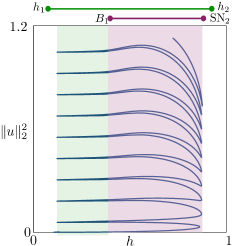
Fig. 13: Bifurcation diagram for $a=1.2$, $\nu=50$, $\varepsilon=1$. Reference intervals for the Heaviside case are reported on top of the bifurcation diagram. The branches occupy a wide region of parameter space, as we expect from the extended bistability region of periodic solutions for high values of $a$ (see panel (b) for $a=1$ in Figure 5)

In order to understand the occurrence of such curves we return to the Heaviside case and concentrate on the even- and odd-symmetric solutions featuring a threshold crossing followed by a threshold tangency at a local minimum (for an example with large $L$, see pattern $1$ in Figure 10). More precisely, we denote by $x_{\ast}$ the point with largest absolute value at which $q_{\textrm{b}}$ attains a local minimum and solve for $(a,h,x_{\ast})$ the system

$$q_{\textrm{b}}(x_{\ast})-q_{\textrm{b}}(x_{0}+L/2)=0$$ (45)

$$q_{\textrm{b}}(x_{\ast})-h=0$$ (46)

$$q_{\textrm{b}}^{\prime}(x_{\ast})=0$$ (47)

where $q_{\textrm{b}}$ is given by Equation (34). We follow solutions to the system above as $L$ varies in a given range and show the corresponding loci of solutions in the $(a,h)$-plane in Figure 10: the dashed curve $T_{\textrm{w}}$ contains solutions to (45)–(47) with a wide active domain ($L$ varies approximately between $45$ and $57$), whereas $T_{\textrm{n}}$ corresponds to solutions with a narrow active domain ($L$ varies approximately between $0.7$ and $12$). Even though $T_{\textrm{w}}$ and $T_{\textrm{n}}$ are not loci of bifurcations, they are indicative of regions of parameter space where solutions with multiple threshold crossings may occur.

In Figure 12 we show a bifurcation diagram for $a=0.8$ for the steep sigmoid: the snaking branch is composed by solutions with two (green), six (blue) or more (magenta) threshold crossings. The snaking structure reflects these three types of solutions and their occurrence is predicted adequately by the two-parameter bifurcation analysis for Heaviside case (reference intervals are reported on top of the bifurcation diagram of Figure 12). Stable and unstable branches alternate in the usual manner and an intertwined branch of localized odd solutions exists as well (not shown). A similar scenario, with an even wider snaking diagram, is found for $a=1.2$ (see Figure 13): for large modulation amplitudes, the bifurcation diagram also contains cross-threshold solutions, but this time their occurrence is marked by the grazing point $B_{1}$ and the saddle nodes $SN_{2}$ (see also the bifurcation diagram for $a=1$ in Figure 5(b)).

8 Conclusions

In the present paper we have studied the existence and bifurcation structure of stationary localized solutions to a neural field model with inhomogeneous synaptic kernel. For Heaviside firing rates, we computed localized as well as spatially-periodic solutions and we followed them in parameter space. We recovered the classical snakes and ladders structure that is found in the one-dimensional Swift–Hohenberg equation as well as previous studies in neural field models: for our model, however, both solutions and bifurcation equations are found analytically. Since linear stability can also be inferred with a simple calculation, it is possible to draw the snaking bifurcation diagrams analytically or semi-analytically (using elementary quadrature rules for the integrals).

Interestingly, we found that the interpretation of the snake and ladder structure proposed by Beck and co-workers [5] and extended by Makrides and Sandstede [45] is valid for the specific inhomogeneous case presented here, for both Heaviside and sigmoidal firing rates: it seems plausible that their framework could be extended to tackle the corresponding non-autonomous spatial-dynamical formulation (11).

With reference to the particular system presented here, we found that a harmonic modulation with an $\mathcal{O}(1)$ spatial wavelength promotes the formation of snaking localized bumps and we note that these structures are driven entirely by the inhomogeneity: in the translation-invariant case, $a=0$, the system supports localized fronts belonging to a non-snaking branch (a scenario that is also found in the homogeneous Swift–Hohenberg equation [37, 3])

We also remark that, in a wide region of parameter space, $a\leq 1$, the kernel is purely excitatory, yet snaking stable bumps are supported. When $a$ is further increased and the kernel becomes excitatory-inhibitory ($a>1$), the snaking limits become wider and involve solutions with multiple threshold crossings. We note that with a modulated but translation-invariant kernel, $A(x-y)$, the integral over the resulting kernel, $W(x)$ would be monotonically increasing and would then prevent the formation of stable bumps for $a<1$ [40]. The inhomogeneity is thus a key ingredient to produce stable solutions in the absence of inhibition when $a<1$.

The analytical methods presented in this paper could be useful in the future to study time-periodic spatially-localized structures (often termed oscillons). A simple mechanism to obtain oscillatory instabilities in neural field models is by introducing linear adaptation [50]. This modification seems amenable to study oscillons, since localized bumps of the extended system can be constructed in the same way presented in this paper, yet the corresponding stability problem changes slightly and may lead to a Hopf bifurcation of the localized steady states. This approach has recently been used by Folias and Ermentrout [27] and Coombes and co-workers [18] in two component models supporting breathers and other spatio-temporal patterns. Another possible extension is to study the effect of spatial modulation in planar neural field models, in which case one could build upon the interface method developed in [19] for homogeneous planar neural fields.

Appendix A Cell reduction for spatially-periodic states

We aim to show that $2\pi\varepsilon$-periodic solutions $q$ to the integral model satisfy

$$q(x)=\int_{-\pi\varepsilon}^{\pi\varepsilon}\tilde{w}(|x-y|)A(y)f(q(y))\mathop{}\!\mathrm{d}y,\qquad x\in[-\pi\varepsilon,\pi\varepsilon)$$

where

$$\widetilde{w}(|x-y|)=\frac{1}{2}{\rm e}^{-|x-y|}+\frac{{\rm e}^{-2\pi\varepsilon}}{1-{\rm e}^{-2\pi\varepsilon}}\cosh\left(|x-y|\right),$$

which correspond to Equations (17) and (19) in the main text.

For exponential kernels $w(|x-y|)=\exp(-|x-y|)/2$, Equation (5) can be rewritten as

$$q(x) = \sum_{m=-\infty}^{-1}\int_{(2m-1)\pi\varepsilon}^{(2m+1)\pi\varepsilon}\frac{1}{2}{\rm e}^{-x+y}A(y)f(q(x-y))\mathop{}\!\mathrm{d}y$$

$$+\sum_{m=1}^{\infty}\int_{(2m-1)\pi\varepsilon}^{(2m+1)\pi\varepsilon}\frac{1}{2}{\rm e}^{x-y}A(y)f(q(x-y))\mathop{}\!\mathrm{d}y$$

$$+\int_{-\pi\varepsilon}^{\pi\varepsilon}\frac{1}{2}{\rm e}^{-|x-y|}A(y)f(q(x-y))\mathop{}\!\mathrm{d}y.$$

By setting $\eta=y-2m\pi\varepsilon$,

$$q(x) = \sum_{m=-\infty}^{-1}\int_{-\pi\varepsilon}^{\pi\varepsilon}\frac{1}{2}{\rm e}^{-x+\eta}{\rm e}^{2m\pi\varepsilon}A(\eta)f(q(x-\eta))\mathop{}\!\mathrm{d}\eta$$

$$+\sum_{m=1}^{\infty}\int_{-\pi\varepsilon}^{\pi\varepsilon}\frac{1}{2}{\rm e}^{x-\eta}{\rm e}^{-2m\pi\varepsilon}A(\eta)f(q(x-\eta))\mathop{}\!\mathrm{d}\eta$$

$$+\int_{-\pi\varepsilon}^{\pi\varepsilon}\frac{1}{2}{\rm e}^{-|x-\eta|}A(\eta)f(q(x-\eta))\mathop{}\!\mathrm{d}\eta.$$

Here, we have made use of the fact that $q(x)$ and $A(x)$ are $2\pi\varepsilon$-periodic functions. Since

$$\sum_{m=-\infty}^{-1}{\rm e}^{2m\pi\varepsilon}=\sum_{m=1}^{\infty}{\rm e}^{-2m\pi\varepsilon}=\frac{{\rm e}^{-2\pi\varepsilon}}{1-{\rm e}^{-2\pi\varepsilon}}.$$

we obtain the reduced formulation (17) with amended kernel (19).

Appendix B Explicit solutions for cross-threshold solutions $q(x)$

An explicit solution for equation (22) with Heaviside nonlinearity and kernel (2) is found by carrying out a direct integration, which gives

$$q_{\textrm{ct}}(x)=\begin{cases}\left({\rm e}^{x}+\dfrac{2{\rm e}^{-2\pi\varepsilon}}{1-{\rm e}^{-2\pi\varepsilon}}\cosh x\right)\Xi(L)&\mbox{if}\quad-\pi\varepsilon<x<-L/2\\ 1+\dfrac{a\varepsilon^{2}}{\varepsilon^{2}+1}\cos\dfrac{x}{\varepsilon}+2\cosh x\left(\dfrac{{\rm e}^{-2\pi\varepsilon}}{1-{\rm e}^{-2\pi\varepsilon}}\Xi(L)+\Upsilon(L)\right)&\mbox{if}\quad-L/2<x<L/2\\ \left({\rm e}^{-x}+\dfrac{2{\rm e}^{-2\pi\varepsilon}}{1-{\rm e}^{-2\pi\varepsilon}}\cosh x\right)\Xi(L)&\mbox{if}\quad L/2<x<\pi\varepsilon\par\end{cases}.$$ (48)

Here,

$$\Xi(L)=\left(\sinh\frac{L}{2}\left(1+\frac{a\varepsilon^{2}}{\varepsilon^{2}+1}\cos\frac{L}{2\varepsilon}\right)+\frac{a\varepsilon}{\varepsilon^{2}+1}\cosh\frac{L}{2}\sin\frac{L}{2\varepsilon}\right),$$ (49)

and

$$\Upsilon(L)={\rm e}^{-L/2}\left(1+\frac{a\varepsilon^{2}}{\varepsilon^{2}+1}\cos\frac{L}{2\varepsilon}-\frac{a\varepsilon}{\varepsilon^{2}+1}\sin\frac{L}{2\varepsilon}\right).$$ (50)

The bifurcation equation is thus given by

$$h=\left({\rm e}^{-L/2}+\frac{2{\rm e}^{-2\pi\varepsilon}}{1-{\rm e}^{-2\pi\varepsilon}}\cosh\frac{L}{2}\right)\times\Xi(L).$$ (51)

References

- [1] S. Amari. Homogeneous nets of neuron-like elements. Biological Cybernetics, 17(4):211–220, 1975.
- [2] S. Amari. Dynamics of pattern formation in lateral-inhibition type neural fields. Biological Cybernetics, 27:77–87, 1977.
- [3] D. Avitabile, D. J. B. Lloyd, J. Burke, E. Knobloch, and B. Sandstede. To snake or not to snake in the planar Swift-Hohenberg equation. SIAM J. Appl. Dyn. Syst., 9:704–733, 2010.
- [4] C. Beaume, A. Bergeon, and E. Knobloch. Convectons and secondary snaking in three-dimensional natural doubly diffusive convection. Physics of Fluids (1994-present), 25(2):024105, February 2013.
- [5] M. Beck, J. Knobloch, D.J.B. Lloyd, B. Sandstede, and T. Wagenknecht. Snakes, ladders, and isolas of localised patterns. SIAM J. Math. Anal, 41(3):936–972, 2009.
- [6] R. Ben-Yishai, R. L. Bar-Or, and H. Sompolinsky. Theory of orientation tuning in visual cortex. Proceedings of the National Academy of Sciences, 92(9):3844–3848, 1995.
- [7] P. C. Bressloff. Traveling fronts and wave propagation failure in an inhomogeneous neural network. Physica D: Nonlinear Phenomena, 155(1):83–100, 2001.
- [8] P. C. Bressloff. Spatiotemporal dynamics of continuum neural fields. Journal of Physics A: Mathematical and Theoretical, 45, 2012.
- [9] P. C. Bressloff, J.D. Cowan, M. Golubitsky, and P.J. Thomas. Scalar and pseudoscalar bifurcations motivated by pattern formation on the visual cortex. Nonlinearity, 14:739, 2001.
- [10] P. C. Bressloff, S. E. Folias, A. Prat, and Y. X. Li. Oscillatory waves in inhomogeneous neural media. Physical Review Letters, 2003.
- [11] J. Burke and E. Knobloch. Homoclinic snaking: structure and stability. Chaos, 17(3):7102, 2007.
- [12] J. Burke and E. Knobloch. Snakes and ladders: localized states in the Swift–Hohenberg equation. Physics Letters A, 360(6):681–688, 2007.
- [13] A. R. Champneys and B. Sandstede. Numerical computation of coherent structures. In Numerical Continuation Methods for Dynamical Systems, pages 331–358. Springer, 2007.
- [14] S. Coombes. Waves, bumps, and patterns in neural field theories. Biological Cybernetics, 93(2):91–108, 2005.
- [15] S. Coombes. Large-scale neural dynamics: Simple and complex. NeuroImage, 52:731–739, 2010.
- [16] S. Coombes and C. R. Laing. Pulsating fronts in periodically modulated neural field models. Physical Review E, 83(1):011912, 2011.
- [17] S. Coombes, G.J. Lord, and M.R. Owen. Waves and bumps in neuronal networks with axo-dendritic synaptic interactions. Physica D: Nonlinear Phenomena, 178(3-4):219–241, 2003.
- [18] S. Coombes, H. Schmidt, and D. Avitabile. Neural Field Theory, chapter Spots: Breathing, drifting and scattering in a neural field model. Springer, 2014.
- [19] S. Coombes, H. Schmidt, and I. Bojak. Interface dynamics in planar neural field models. Journal of mathematical neuroscience, 2012.
- [20] S. Coombes, N. A. Venkov, L. Shiau, I. Bojak, D. T. J. Liley, and C. R. Laing. Modeling electrocortical activity through improved local approximations of integral neural field equations. Physical Review E, 76:051901, 2007.
- [21] P. Coullet, C. Riera, and C. Tresser. Stable static localized structures in one dimension. Phys. Rev. Lett., 84(14):3069–3072, 3 April 2000.
- [22] J. H. P Dawes. Localized Pattern Formation with a Large-Scale Mode: Slanted Snaking. SIAM J. Appl. Dyn. Syst., 7(1):186–206, February 2008.
- [23] G. B. Ermentrout and J. D. Cowan. A mathematical theory of visual hallucination patterns. Biological Cybernetics, 34(3):137–150, 1979.
- [24] G. B. Ermentrout and D Kleinfeld. Traveling electrical waves in cortex: Insights from phase dynamics and speculation on a computational role. Neuron, 29:33–44, 2001.
- [25] G. Faye, J. Rankin, and P. Chossat. Localized states in an unbounded neural field equation with smooth firing rate function: a multi-parameter analysis. Journal of Mathematical Biology, pages 1–36, 2012.
- [26] G. Faye, J. Rankin, and D. J. B. Lloyd. Localized radial bumps of a neural field equation on the euclidean plane and the poincaré disk. Nonlinearity, 26(2):437, 2013.
- [27] S. E. Folias and G. B. Ermentrout. Bifurcations of Stationary Solutions in an Interacting Pair of E-I Neural Fields. SIAM J. Appl. Dyn. Syst., 11(3):895–938, 2012.
- [28] P. S. Goldman-Rakic. Cellular basis of working memory. Neuron, 14:477–485, 1995.
- [29] W. J. F. Govaerts. Numerical Methods for Bifurcations of Dynamical Equilibria. SIAM, January 2000.
- [30] D. Hansel and H. Sompolinsky. Modeling feature selectivity in local cortical circuits. Methods of neuronal modeling, pages 499–567, 1997.
- [31] D. H. Hubel and T. N. Wiesel. Receptive fields, binocular interaction and functional architecture in the cat’s visual cortex. Journal of Physiology, 160:106–154, 1962.
- [32] D. H. Hubel and T. N. Wiesel. Receptive fields and functional architecture of monkey striate cortex. Journal of Physiology, 195:215–243, 1968.
- [33] D. H. Hubel and T. N. Wiesel. Sequence regularity and geometry of orientation columns in the monkey striate cortex. Journal of Comparative Neurology, 158:267–293, 1974.
- [34] D. H. Hubel and T. N. Wiesel. Functional architecture of macaque monkey visual cortex. Proceedings of the Royal Society of London, Series B, Biological Sciences, 198:1–59, 1977.
- [35] H. C. Kao, C. Beaume, and E. Knobloch. Spatial localization in heterogeneous systems. Physical Review E, 89:012903, 2014.
- [36] U. Kim, T. Bal, and D. A. McCormick. Spindle waves are propagating synchronized oscillations in the ferret LGNd in vitro. Journal of Neurophysiology, 74:1301–1323, 1995.
- [37] J. Knobloch and T. Wagenknecht. Homoclinic snaking near a heteroclinic cycle in reversible systems. Physica D: Nonlinear Phenomena, 206(1-2):82–93, June 2005.
- [38] C. L. Laing, W. C. Troy, B. Gutkin, and G. B. Ermentrout. Multiple bumps in a neuronal model of working memory. SIAM J. Appl. Math., 63(1):62–97, 2002.
- [39] C. R. Laing. Neural Field Theory, chapter PDE Methods for Two-Dimensional Neural Fields. Springer, 2013.
- [40] C. R. Laing and W. C. Troy. PDE methods for nonlocal models. SIAM Journal on Applied Dynamical Systems, 2(3):487–516, 2003.
- [41] M. Lauritzen. Pathophysiology of the migraine aura. The spreading depression theory. Brain, 117:199–210, 1994.
- [42] D. J. B. Lloyd and B. Sandstede. Localized radial solutions of the Swift-Hohenberg equation. Nonlinearity, 22(2):485–524, 2009.
- [43] D. J. B. Lloyd, B. Sandstede, D. Avitabile, and A. R. Champneys. Localized hexagon patterns of the planar Swift–Hohenberg equation. SIAM J. Appl. Dyn. Syst., 7:1049–1100, 2008.
- [44] D. Lo Jacono, A. Bergeon, and E. Knobloch. Three-dimensional spatially localized binary-fluid convection in a porous medium. Journal of Fluid Mechanics, 730:R2, 2013.
- [45] E. Makrides and B. Sandstede. Predicting the bifurcation structure of localized snaking patterns. Physica D, 268:59–78, 2014.
- [46] S. McCalla and B. Sandstede. Snaking of radial solutions of the multi-dimensional Swift-Hohenberg equation: A numerical study. Physica D, 239(16):1581–1592, 2010.
- [47] R. Miles, R. D. Traub, and R. K. Wong. Spread of synchronous firing in longitudinal slices from the CA3 region of Hippocampus. Journal of Neurophysiology, 60:1481–1496, 1988.
- [48] D. Morgan and J. H. P Dawes. The Swift–Hohenberg equation with a nonlocal nonlinearity. Physica D, 270:60–80, March 2014.
- [49] L. Muller and A. Destexhe. Propagating waves in thalamus, cortex and the thalamocortical system: Experiments and models. Journal of Physiology-Paris, 106:222–238, 2012.
- [50] D. J. Pinto and G. B. Ermentrout. Spatially structured activity in synaptically coupled neuronal networks: 2. standing pulses. SIAM J. of Appl. Math., 62:226–243, 2001.
- [51] J. Rankin, D. Avitabile, J. Baladron, G. Faye, and D. J. B. Lloyd. Continuation of localised coherent structures in nonlocal neural field equations. SIAM J. Sci. Comput., 36(1):B70–B93, 2013.
- [52] H. Sakaguchi and H. R. Brand. Stable localized solutions of arbitrary length for the quintic Swift-Hohenberg equation. Physica D, 97(1-3):274–285, 1996.
- [53] H. Sakaguchi and H. R. Brand. Localized patterns for the quintic complex Swift-Hohenberg equation. Physica D, 117(1-4):95–105, 1998.
- [54] T. K. Sato, I. Nauhaus, and M. Carandini. Traveling Waves in Visual Cortex. Neuron, 75(2):218–229, 2012.
- [55] H. Schmidt, A. Hutt, and L. Schimansky-Geier. Wave fronts in inhomogeneous neural field models. Physica D, 238(14):1101–1112, 2009.
- [56] T. Schneider, J. F Gibson, and J. Burke. Snakes and ladders: localized solutions of plane Couette flow. Phys. Rev. Lett., 104(10):104501, 2010.
- [57] H. R. Wilson and J. D. Cowan. Excitatory and inhibitory interactions in localized populations of model neurons. Biophys. J., 12:1–24, 1972.
- [58] H. R. Wilson and J. D. Cowan. A mathematical theory of the functional dynamics of cortical and thalamic nervous tissue. Biological Cybernetics, 13(2):55–80, September 1973.
- [59] P. D. Woods and A. R. Champneys. Heteroclinic tangles and homoclinic snaking in the unfolding of a degenerate reversible hamiltonian-hopf bifurcation. Physica D: Nonlinear Phenomena, 129(3-4):147–170, 1999.
- [60] J. Y. Wu, L. Guan, and Y. Tsau. Propagating activation during oscillations and evoked responses in neocortical slices. Journal of Neuroscience, 19:5005–5015, 1999.