The nature of supernovae 2010O and 2010P in Arp 299 - II. Radio emission

Abstract

We report radio observations of two stripped-envelope supernovae (SNe), 2010O and 2010P, which exploded within a few days of each other in the luminous infrared galaxy Arp 299. Whilst SN 2010O remains undetected at radio frequencies, SN 2010P was detected (with an astrometric accuracy better than 1 milli arcsec in position) in its optically thin phase in epochs ranging from $\sim 1$ to $\sim 3$ yr after its explosion date, indicating a very slow radio evolution and a strong interaction of the SN ejecta with the circumstellar medium. Our late-time radio observations toward SN 2010P probe the dense circumstellar envelope of this SN, and imply $\dot{M}[\,\mbox{$\mathrm{M_{\sun}\,yr^{-1}}$}{}]/v_{\mathrm{wind}}[10\,\,\mbox{$\mathrm{km\,s^{-1}}$}{}]=(3.0$–5.1)$\times 10^{{-}{5}}$, with a 5 GHz peak luminosity of $\sim 1.2\mbox{$\times 10^{{2}{7}}$}$ $\,\mathrm{erg\,s^{-1}\,Hz^{-1}}$ on day $\sim$464 after explosion. This is consistent with a Type IIb classification for SN 2010P, making it the most distant and most slowly evolving Type IIb radio SN detected to date.

1 Introduction

Core-collapse supernovae (CCSNe) are the signposts of recent massive star formation. Since much of the massive star formation is embedded in dust, a substantial fraction of the CCSNe in the Universe will remain hidden in optical searches (Mattila et al., 2012). This is particularly true in the case of star formation taking place in the dusty environments of luminous ($10^{11}\,\,\mbox{$\mathrm{L_{\sun}}$}{}<L_{\mathrm{IR}}{}<10^{12}\,\,\mbox{$\mathrm{L_{\sun}}$}{}$), and ultra-luminous ($L_{\mathrm{IR}}{}>10^{12}\,\,\mbox{$\mathrm{L_{\sun}}$}{}$) infrared (IR) galaxies (LIRGs and ULIRGs, respectively), which dominates the star formation rate density at $z>1$ (e.g., Magnelli et al., 2011). In many LIRGs, the bulk of star formation occurs within their circumnuclear regions ($<1$ kpc), so that the need for high-resolution observations becomes crucial in the detection and study of CCSNe therein.

The synergy between high resolution radio and near-infrared (NIR) K-band (where the extinction is 10 times lower than in the optical) observations is currently being used to help build a complete picture of the supernova (SN) activity in dusty starbursts and LIRGs. Outstanding examples are SNe 2000ft (in NGC 7469; Pérez-Torres et al., 2009a, and references therein), 2004ip (in IRAS 18293$-$3413; Mattila et al., 2007; Pérez-Torres et al., 2007), 2008cs (in IRAS 17138$-$1017; Kankare et al., 2008), and 2008iz (in M82; Brunthaler et al., 2009; Mattila et al., 2013) where both high resolution (to disentangle the emission of the SN from its host) and reduced extinction measurements (radio and NIR), were essential in their detection and characterisation.

Arp 299 is a LIRG with an IR luminosity ($L_{\mathrm{IR}}\approx 6.7\mbox{$\times 10^{{1}{1}}$}$ L_☉ (Sanders et al., 2003), at an adopted luminosity distance of 44.8 Mpc, assuming $H_{0}=73$ km s^-1 Mpc^-1. The system is composed of two interacting galaxies, whose major nuclei (A and B1) and core components in the interacting region (C^′ and C) are bright radio and NIR emitters (Gehrz, Sramek, & Weedman, 1983; Alonso-Herrero et al., 2000). Arp 299 is a very prolific SN factory as proved by the detection of several radio SNe and SN remnants (SNRs) in the innermost nuclear regions of Arp 299A and Arp 299B (Pérez-Torres et al., 2009b; Ulvestad, 2009; Romero-Cañizales et al., 2011; Bondi et al., 2012), and the detection within the last 20 years of seven optical/NIR SNe in the circumnuclear regions of the system (see Anderson, Habergham, & James, 2011; Mattila et al., 2012).

Many attempts have been made to detect at radio wavelengths the SNe occurring in the circumnuclear regions of Arp 299, mostly under observing programmes with the Very Large Array (VLA): AS333 carried out from 1990 May to 1993 December; AS525 on 1994 February to detect SN 1993G; AS568 on 1999 January, February, April and October to detect SN 1999D; AW641 on 2005 February, June and August to detect SN 2005U. We are currently monitoring Arp 299 at radio wavelengths under programmes AP592 and AP614, “Unveiling the Hidden Population of SNe in Local Luminous Infrared Galaxies” (PI: M. A. Pérez-Torres), as part of a combined radio and NIR SN search in a sample of local LIRGs. In this paper we study the nature of the most recently detected SNe in the system, 2010O and 2010P, by means of their late-time radio emission.

SN 2010O was discovered at optical wavelengths on 2010 January 24 (Newton, Puckett, & Orff, 2010). The object exploded on 2010 January 7 and lies on a location with intermediate extinction, $A_{V}=2$ mag (Kankare et al. 2013). It was classified as a Type Ib SN by Mattila et al. (2010) based on a low-resolution optical spectrum obtained with the Nordic Optical Telescope (NOT). Nelemans et al. (2010) reported an X-ray transient at the position of SN 2010O prior to its explosion, and suggested that the progenitor of this SN was part of a Wolf-Rayet X-ray binary system, similar to those found in our Galaxy.

SN 2010P was discovered at NIR wavelengths with the NOT on 2010 January 18 (Mattila & Kankare, 2010), a few days after explosion (2010 January 10, Kankare et al. 2013). The spectrum of SN 2010P obtained with the Gemini-North Telescope revealed a deficiency of hydrogen and matched with spectra of Type Ib/IIb SNe (Ryder et al., 2010), and the absolute magnitude and colours from optical and NIR observations with the NOT and the Gemini-North Telescope yielded a likely high host galaxy extinction of $A_{V}\sim 7$ (Kankare et al. 2013).

This paper accompanies Paper I by Kankare et al. (2013) which presents a study of the early optical and NIR emission of SNe 2010O and 2010P. Here we analyse long-term follow-up radio observations of Arp 299 carried out by us and obtained from archives, with particular emphasis on characterising SNe 2010O and 2010P. In Section 2 we give details on the data reduction and analysis. We describe our results in Section 3, which we then discuss in Section 4. In Section 5 we summarize the conclusions of our work.

2 Radio observations

We have collected observations of Arp 299 obtained with the Multi-Element Radio Linked Interferometry Network (MERLIN), the electronic Multi-Element Remotely Linked Interferometer Network (e-MERLIN), the VLA of the National Radio Astronomy Observatory (NRAO), and the European very long baseline interferometry (VLBI) Network (EVN). In Table 1 we show basic information for these observations (all of which have an assigned label) including the range of frequencies observed, the total time on target ($t_{\mathrm{on}}$), and the peak intensity in each epoch of J1128$+$5925, which was used as the phase calibrator in all the observations we report here.

Table 1: Arp 299 radio observations.

Label	Project	Observing	Frequency range	Array / Participating stations	$t_{\mathrm{on}}$	$P_{\nu}$[J1128$+$5925]
		date	(MHz)			( $\mathrm{Jy/beam}$)
E1	-	2010-01-29/02-01	4986–5002	MERLIN / Mk2, Kn, De, Pi, Da, Cm	29 h	0.44 $\pm$ 0.02
E2	AL746	2011-03-29	28500–29500	VLA - B configuration	6 m	0.31 $\pm$ 0.02
E3	AL746	2011-03-29	35500–36500	VLA - B configuration	6 m	0.28 $\pm$ 0.01
E4	AP592	2011-06-15/06-18	8372–8628	VLA - A configuration	19 m	0.44 $\pm$ 0.05
E5	-	2011-07-04	4444–4956	e-MERLIN / Mk2, Kn, De, Pi, Da	25 h	0.40 $\pm$ 0.10
E6	EP075B	2012-05-27	8344–8472	EVN / Ef, Wb, On, Mc, Nt, Ur, Ys, Sv, Zc	4.3 h	0.42 $\pm$ 0.02
E7	EP075C	2012-06-04	4919–5047	EVN / Ef, Wb, Jb1, On, Mc, Nt, Tr, Ur, Ys, Sv, Zc, Bd	2.7 h	0.50 $\pm$ 0.03
E8	EP075D	2012-06-14	1587–1715	EVN / Ef, Wb, Jb1, On, Mc, Nt, Tr, Ur, Sv, Zc, Bd	2.9 h	0.36 $\pm$ 0.02
E9	AP614	2012-10-20	7395–9395	VLA - A configuration	19 m	0.62 $\pm$ 0.03
E10	EP075E	2012-10-31	4919–5047	EVN / Ef, Wb, Jb2, On, Mc, Tr, Ur, Ys, Bd, Sh	4.4 h	0.58 $\pm$ 0.03
E11	AP614	2012-11-05	7395–9395	VLA - A configuration	19 m	0.60 $\pm$ 0.03
E12	AP614	2012-11-21	7395–9395	VLA - A configuration	19 m	0.62 $\pm$ 0.03
E13	AP614	2012-12-26	7395–9395	VLA - A configuration	19 m	0.59 $\pm$ 0.03

Last column: Peak intensity of the phase reference source.

The reduction and analysis for MERLIN, e-MERLIN and EVN data were made following standard procedures within the NRAO Astronomical Image Processing System (aips); for the VLA data, we used the Common Astronomy Software Applications package (casa; McMullin et al., 2007).

Epoch E1 with MERLIN (PI: M. A.  Pérez-Torres) was obtained in an attempt to detect the early radio emission of SNe 2010O and 2010P (results reported in Beswick et al., 2010). Observations of 3C 286 and OQ208 were used for absolute flux density and bandpass calibration.

We used publicly available Ka-band VLA data taken in B configuration (maximum antenna separation of $\approx 11$ km) under project AL746 (PI: A. K. Leroy), which include two sub-bands at 29.0 and 36.0 GHz, which we labelled for convenience E2 and E3, respectively, although these observations were obtained at the same epoch. 3C 286 was observed for absolute flux density calibration. To obtain the final image, we applied standard imaging procedures and two iterations of phase-only self-calibration on the target. Since we were interested in a possible detection of the SN, we applied natural weighting to the data to minimise the root mean square (rms).

We observed Arp 299 with the VLA in its most extended configuration, A ($\approx 36$ km as the maximum antenna separation), under program AP592, and labelled here as epoch E4 (the first radio detection of SN 2010P; Herrero-Illana et al., 2012). For imaging we followed the same procedure as for epochs E2 and E3, except for the use of uniform weighting instead of natural, to reduce the effect of confusion with the extended emission (traced by the shortest baselines) at the SN site. This is also true for epochs E9, E11, E12 and E13 which were obtained under program AP614.

Epoch E5 was observed as part of the commissioning observations of e-MERLIN for the Luminous Infrared Galaxy Inventory legacy project (LIRGI; PIs: J., Conway & M. A. Pérez-Torres). The total on-source time was $\sim 25$ hr (see Table 1) but intense data flagging was needed, leaving only $\sim 16$ hr worth of useful data. As amplitude calibrators we observed 3C 286, OQ208 and DA193; to correct the bandpass we used DA193 and 1803$+$784, the last one being used also as a fringe finder.

Our EVN observations (epochs E6, E7, E8 and E10) originally were aimed at imaging the Arp 299A and -B1 nuclear regions. After confirming the radio detection of SN 2010P in epoch E4 with the VLA (see Herrero-Illana et al., 2012), we requested the correlation of the EVN observations at the position of the radio SN. For all these epochs, the source 4C39.25 was used as a fringe finder, and also together with J1128$+$5925 as a bandpass calibrator, to ensure having solutions for all the antennas. We used the EVN pipeline products and improved the calibration of the data by removing radio interference artifacts and by including ionospheric corrections. We determined gain corrections for each antenna by imaging the calibrators with the Caltech program difmap (Shepherd, Pearson, & Taylor, 1995), and applied corrections larger than 10 per cent to the uv-data using the aips task clcor. The EVN maps of SN 2010P at the different frequencies were all made with natural weighting.

In Table 2 we show the characteristics of the resultant images, such as the synthesised beam, the attained off-source rms noise, together with other relevant information that will be described in the following sections.

3 Results

SNe 2010O and 2010P were not detected in the MERLIN observations carried out between 2010 January 29 and February 1 at 5.0 GHz (Beswick et al., 2010). However, late-time radio observations have shed light on the nature of these SNe.

Table 2: Observational data measured from the radio images of SN 2010P obtained from the observations described in Table 1.

Label	$t_{\mathrm{obs}}-t_{0}$	$\nu$	rms	FWHM, PA	$S_{\nu}$	$L_{\nu}$	log $T_{\mathrm{B}}$
	(days)	(GHz)	( $\mathrm{\mu Jy/beam}$)	(mas2, $\degr{}$)	( $\mathrm{\mu Jy}$)	($10^{26}$$\,\mathrm{erg\,s^{-1}\,Hz^{-1}}$)	(K)
(1)	(2)	(3)	(4)	(5)	(6)	(7)	(8)
E1	19	5.0	62	$46.4\times 44.1$, $-75.1$	$<186$	-	-
E2	443	29.0	47	$304\times 285$, 86.6	278 $\pm$ 49	6.7 $\pm$ 1.2	$<$0.67 $\pm$ 0.08
E3	443	36.0	83	$305\times 260$, $-69.4$	$<249$	-	-
E4	521	8.5	88	$211\times 151$, 12.7	541 $\pm$ 92	13.0 $\pm$ 2.2	$<$2.46 $\pm$ 0.07
E5	540	4.7	63	$187\times 143$, 47.5	585 $\pm$ 69	14.0 $\pm$ 1.7	$<$3.09 $\pm$ 0.05
E6	868	8.4	18	$2.7\times 1.5$, 21.0	123 $\pm$ 19	3.0 $\pm$ 0.5	$<$6.26 $\pm$ 0.07
E7	876	5.0	17	$4.2\times 3.1$, 34.6	288 $\pm$ 22	6.9 $\pm$ 0.5	$<$6.04 $\pm$ 0.03
E8	886	1.7	15	$17.3\times 8.1$,7.9	466 $\pm$ 28	11.2 $\pm$ 0.7	$<$6.17 $\pm$ 0.03
E9	1014	8.5	51	$226\times 135$, 59.7	259 $\pm$ 52	6.2 $\pm$ 1.3	$<$2.16 $\pm$ 0.09
E10	1025	5.0	13	$6.2\times 3.9$,$-78.0$	284 $\pm$ 19	6.8 $\pm$ 0.5	$<$5.76 $\pm$ 0.03
E11	1030	8.5	46	$188\times 136$,$-177.2$	270 $\pm$ 48	6.5 $\pm$ 1.2	$<$2.26 $\pm$ 0.08
E12	1046	8.5	41	$183\times 138$, 8.7	195 $\pm$ 42	4.7 $\pm$ 1.0	$<$2.12 $\pm$ 0.09
E13	1081	8.5	43	$225\times 133$, 62.6	251 $\pm$ 45	6.0 $\pm$ 1.1	$<$2.15 $\pm$ 0.08

Columns: (1) Epoch label. (2) Days since explosion. (3) Observing central frequency. (4) rms noise. (5) Full width at half maximum (FWHM) synthesised interferometric beam. (6) Flux density. (7) Monochromatic luminosity at the observing frequency. (8) Brightness temperature. To calculate the solid angle subtended by the SN we used the major and minor axes from column 5, except for epoch E6 where we could obtain the deconvolved size by means of a Gaussian fitting with the aips task imfit.

3.1 The radio non-detection of SN 2010O

In Paper I we determined that SN 2010O exploded on 2010 January 7. We do not detect it in either early- ($\sim 0.6$ month) or late-time ($\sim 1$ to $\sim 3$ yr after the explosion) radio observations reported by Beswick et al. (2010) and in this paper, respectively. The MERLIN observations (E1 at $\sim 0.6$ month) by Beswick et al. resulted in a $3\sigma$ upper limit of 186 $\mathrm{\mu Jy/beam}$ for the radio emission of SN 2010O, i.e., a luminosity $<4.5\mbox{$\times 10^{{2}{6}}$}$ $\,\mathrm{erg\,s^{-1}\,Hz^{-1}}$. The most sensitive late-time epoch we present here which covers the SN 2010O region (E12 at 2.8 yr), results in a $3\sigma$ upper limit of 123 $\mathrm{\mu Jy/beam}$ ($<3\mbox{$\times 10^{{2}{6}}$}$ $\,\mathrm{erg\,s^{-1}\,Hz^{-1}}$). Our results suggest that: i) the SN was intrinsically weak, with a luminosity $<3\mbox{$\times 10^{{2}{6}}$}$ $\,\mathrm{erg\,s^{-1}\,Hz^{-1}}$; and/or ii) its radio emission was heavily absorbed by the dense CSM at the moment of the early-time MERLIN observations, and owing to a fast-evolving nature, its short radio lifetime prevented its detection in our late-time radio observations.

3.2 The radio emission of SN 2010P

In Herrero-Illana et al. (2012) we reported the identification of SN 2010P with a new high signal-to-noise ratio (S/N$>10$) radio source in our 8.5 GHz VLA map from 2011 June 15-18 (E4), matching the NIR position within its 1$\sigma$ uncertainty reported by Mattila & Kankare (2010). No radio source is visible at that position in any of the 14 VLA epochs from 1990 to 2006 analysed by Romero-Cañizales et al. (2011). The radio detection of SN 2010P is confirmed by our e-MERLIN (4.7 GHz) and EVN observations (at 1.7, 5.0 and 8.4 GHz), and by the archival VLA data, all of these made during 2011 and 2012.

Figure 1: Top: e-MERLIN contour image of Arp 299 at a median central frequency of 4.7 GHz with an rms noise of 63  $\mathrm{\mu Jy/beam}$. The main radio sites are indicated with the letters A, B, C^′ and C, the position of SN 2010O is represented by a cross, and SN 2010P is enclosed by a box. Bottom: EVN contour images of SN 2010P at a median central frequency of 8.4, 5.0 and 1.7 GHz (from left to right). All the EVN maps are centred at $\alpha(J2000)=11\mathrm{{}^{h}}28\mathrm{{}^{m}}31\aas@@fstack{s}3605$, $\delta(J2000)=58\degr 33\arcmin 49\aas@@fstack{\prime\prime}315$. The rms noise in each EVN image is 18, 17 and 15  $\mathrm{\mu Jy/beam}$, respectively. The beam size is shown in the lower left corner of each contour image.

In Table 2 we report the parameters measured from our radio maps at the position of SN 2010P (e-MERLIN and EVN maps are shown in Figure 1). We include the convolving beam, as well as the attained rms and the flux density measurements in each map. Since the SN remains unresolved in all the epochs, we take its measured peak intensity as a good approximation for the flux density, whose uncertainty includes the contributions of the rms and a systematic 5 per cent uncertainty in the absolute flux calibration. For the images presented in Figure 1 we modified the pixel size of the maps (from epochs E6, E7 and E8) to match that of the lowest resolution map obtained at 1.7 GHz, using the task ohgeo within aips.

The luminosities obtained in the late time observations are typical of normal CCSNe. The fact that the SN is detected $\sim 1$ yr after explosion and that it has remained radio bright for about two years (the time between epochs E2 and E13), indicates a slow radio evolution and thus the presence of either a dense and/or extended circumstellar medium (CSM).

At an age of 2.4 and 2.8 yr (epochs E6 to E8 and E10) the $T_{\mathrm{B}}$ values indicate that the radio emission is non-thermal at the three different frequencies observed with the EVN, and corresponds to a compact object of 2.0 $\times$ 0.6 mas² (deconvolved size) at $\alpha(J2000)=11\mathrm{{}^{h}}28\mathrm{{}^{m}}31\aas@@fstack{s}3605\pm 0.2$ mas, $\delta(J2000)=58\degr 33\arcmin 49\aas@@fstack{\prime\prime}315\pm 0.2$ mas in our 8.4 GHz EVN map (E6), which provides the highest resolution and thus the highest astrometric accuracy. The uncertainty in position has been determined by adding in quadrature $\mathrm{FWHM}/(2\times\mathrm{S/N})$ of the SN, plus the uncertainty in position of the phase reference source ($\Delta\alpha=0.23$ mas, $\Delta\delta=0.13$ mas).

We conservatively take the deconvolved size from epoch E6 to set an upper limit to the size of the expanding ejecta of 1.3 mas in diameter on average, which at a distance of 44.8 Mpc, implies an upper limit of 4.3$\times 10^{{1}{7}}$ cm in radius. For any SN progenitor, such a size would imply that the distance from either the progenitor’s centre or the photosphere to the shock region are basically equal. Thus, even considering free-expansion, it is not possible to set a reliable constraint for the shock velocity.

The $T_{\mathrm{B}}$ values from the VLA and e-MERLIN epochs are consistent with non-thermal emission that is being suppressed owing to thermal and/or non-thermal processes. With a larger beam in those epochs (compared to that from our EVN images) it is likely that the flux of the SN itself and the contaminating emission from the host, will contribute jointly to the flux measurements.

3.2.1 Contaminating emission

A meaningful comparison among epochs with different resolution necessitates an estimate of the background emission affecting the flux density measurements of the low-resolution images. Contamination is likely to occur when observing at angular resolutions comparable to, or only a few times the separation between a SN and its host. This is specially important in this case since SN 2010P exploded very close to component C^′ ($\approx 160$ pc projected distance, or $\approx 720$ mas), which is also a bright radio source and is surrounded by diffuse emission.

The diffuse emission detectable in the different low-resolution epochs (e.g., E5, Figure 1) is limited by the thermal rms in the individual images and the weighting used in the mapping process. The wealth of diffuse emission at the position of SN 2010P is revealed in deep Arp 299 images at different frequencies (e.g., Neff, Ulvestad, & Teng, 2004).

We have co-added all the 8.5 GHz epochs analysed by Romero-Cañizales et al. (2011), and produced a deep image with a convolving beam of $0.21\times 0.14$ arcsec², equal to the average of the convolving beam used in our VLA epochs at 8.5 GHz. We then solved for the zero level emission at the position of SN 2010P using the task imfit within aips, which we then adopted as the background emission at 8.5 GHz for SN 2010P.

We estimate the background emission at 4.7 GHz by applying the fiducial spectral index obtained by Leroy et al. (2011) for Arp 299 ($\alpha=-0.62$), to the background emission at 8.5 GHz. Such a spectral index does not apply to frequencies $\ga 30$ GHz where a higher contribution from thermal emission is expected. Instead, we obtained a representative zero level emission at 29.0 GHz, by measuring it at different positions around the SN location in our E2 image, and then taking the average of the retrieved values. We note that the E2 image was made with natural weighting to facilitate a robust SN detection, and thus some diffuse emission was detectable in it. The background emission at 4.7, 8.5 and 29.0 GHz are given in Table 3.

We subtracted the background emission from epochs E2, E4, E5, E9, E11, E12 and E13, at their corresponding frequencies. We then calculated the E4 to E5 and the E6 to E7 spectral indices, to convert the e-MERLIN flux density to be at 5.0 GHz, and allow its comparison with epochs E1 and E7. Similarly, we converted the E6 flux density to be at 8.5 GHz, for the sake of homogeneity. The corrected flux densities at the adopted frequencies along with the observed parameters (from Table 1) are shown in Table 4 for comparison.

Table 3: Contaminating background emission for SN 2010P.

Frequency	$S_{\nu}$
(GHz)	( $\mathrm{\mu Jy}$)
4.7	178 $\pm$ 10
8.5	123 $\pm$ 7
29.0	200 $\pm$ 23

Table 4: SN 2010P measured and contamination-free flux densities.

Epoch		Observed		Adopted	Corrected
label	$t_{\mathrm{obs}}-t_{0}$	$\nu$	$S_{\nu}$	$\nu$	$S_{\nu}$
	(days)	(GHz)	( $\mathrm{\mu Jy}$)	(GHz)	( $\mathrm{\mu Jy}$)
E1	19	5.0	$<186$	5.0	$<186$
E2	443	29.0	278 $\pm$ 49	29.0	76 $\pm$ 72
E3	443	36.0	$<249$	36.0	$<249$
E4	521	8.5	541 $\pm$ 92	8.5	418 $\pm$ 99
E5	540	4.7	585 $\pm$ 69	5.0	408 $\pm$ 81
E6	868	8.4	123 $\pm$ 19	8.5	122 $\pm$ 19
E7	876	5.0	288 $\pm$ 22	5.0	288 $\pm$ 22
E8	886	1.7	466 $\pm$ 28	1.7	466 $\pm$ 28
E9	1014	8.5	259 $\pm$ 52	8.5	136 $\pm$ 59
E10	1025	5.0	284 $\pm$ 19	5.0	284 $\pm$ 19
E11	1030	8.5	270 $\pm$ 48	8.5	147 $\pm$ 55
E12	1046	8.5	195 $\pm$ 42	8.5	71 $\pm$ 49
E13	1081	8.5	251 $\pm$ 45	8.5	127 $\pm$ 52

Note that the values of some epochs are unchanged, but we show them all for completeness.

3.2.2 Radio spectrum

We have obtained a radio continuum spectrum of SN 2010P at three different ages (Figure 2). We used the corrected flux densities retrieved from the quasi-simultaneous epochs E4 and E5 at 1.4 yr, E6 to E8 at 2.4 yr, and from epochs E9 and E10 at an age of 2.8 yr.

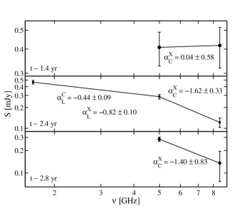
Figure 2: Radio continuum spectrum of SN 2010P at 1.4, 2.4 and 2.8 yr after explosion.

At 1.4 yr, the two-point spectral index $\left(S_{\nu}\propto\nu^{\alpha}\right)$ between 5.0 and 8.5 GHz is $\alpha_{\scriptstyle C}^{\scriptstyle X}(1.4\mathrm{yr})=0.04\pm 0.58$, using the corrected values from Table 4. The resulting 1.7 to 5.0 GHz and 5.0 to 8.5 GHz spectral indices at 2.4 yr are $\alpha_{\scriptstyle L}^{\scriptstyle C}(2.4\mathrm{yr})=-0.44\pm 0.09$, and $\alpha_{\scriptstyle C}^{\scriptstyle X}(2.4\mathrm{yr})=-1.62\pm 0.33$, respectively. At an age of 2.8 yr, the 5.0 to 8.5 GHz spectral index results in $\alpha_{\scriptstyle C}^{\scriptstyle X}(2.8\mathrm{yr})=-1.40\pm 0.83$.

The flat spectral index that we observe at 1.4 yr indicates that the SN emission is becoming transparent at $\sim$500 days after explosion. We note that once a SN reaches its maximum (at time $t_{\mathrm{peak}}$) and enters its optically thin phase, a higher flux density is observed at lower frequencies (Weiler et al., 2002), as we observe for SN 2010P at 2.4 and 2.8 yr. The knee in the spectrum at 2.4 yr would be a consequence of the radio emission being transparent at 5.0 and 8.4 GHz, whilst still being slightly absorbed at 1.7 GHz.

We note that $\alpha_{\scriptstyle C}^{\scriptstyle X}(2.4\mathrm{yr})$ and $\alpha_{\scriptstyle C}^{\scriptstyle X}(2.8\mathrm{yr})$ are highly consistent. However, the latter involves a measurement affected by the galactic background emission unlike the former, and hence it has a larger uncertainty. We thus consider that $\alpha_{\scriptstyle C}^{\scriptstyle X}(2.4\mathrm{yr})$ describes the optically thin phase of the SN more reliably (see Section 3.3).

3.3 The radio light curve of SN 2010P

The shape of a SN light curve is dominated by two main factors: the non-thermal radio emission which declines slowly, and the rapid decline of non-thermal and thermal absorption, mainly, synchrotron self-absorption (SSA) and free-free absorption (FFA). SSA originates at the shocked-CSM region, when the pressure is high enough so that the ultra-relativistic electrons absorb their own synchrotron photons. FFA arises from the ionized medium surrounding the SN, which absorbs the synchrotron photons.

There are a number of models in the literature which allow a successful parametrisation of SN light curves (see e.g., Weiler et al., 2002; Soderberg et al., 2005). Whilst these models include many details on the characteristics of the SN itself and its CSM, a good sampling of the radio emission through time at multiple frequencies is required to constrain all of these parameters.

We make an attempt to parametrise the light curve of SN 2010P using the model described in Weiler et al. (2002). Given that the sampling we have is very limited, we aim to obtain a qualitative view of the SN 2010P radio behaviour when comparing it with other known radio SNe. At the late SN stages covered by our data, we expect that the radio light curves will be dominated by FFA, however, as SSA has been found to be important in the evolution of type Ib/IIb SNe, here we explore both pure SSA and pure FFA models. Whilst a combined SSA and FFA model would be ideal, we note that this is not feasible due to the scarce existing data, specially at early epochs covering the optically thick part of the SN evolution.

Following Weiler et al. (2002), the evolution in time ($t$) of the flux density ($S$) at a frequency ($\nu$) is given by,

$$S[\,\mbox{$\mathrm{mJy}$}]=K_{1}\left(\frac{\nu}{5~{}\mathrm{GHz}}\right)^{\alpha}\left(\frac{t-t_{0}}{1~{}\mathrm{day}}\right)^{\beta}A_{1}~{}A_{2}~{}A_{3}$$ (1)

with

$$A_{1}=e^{-\tau_{\mathrm{external}}};$$

$$A_{2}=\frac{1-e^{-\tau_{\mathrm{CSM}_{\mathrm{clumps}}}}}{\tau_{\mathrm{CSM}_{\mathrm{clumps}}}},$$

where

$$\tau_{\mathrm{external}}=K_{2}\left(\frac{\nu}{5~{}\mathrm{GHz}}\right)^{-2.1}\left(\frac{t-t_{0}}{1~{}\mathrm{day}}\right)^{\delta}+K_{4}\left(\frac{\nu}{5~{}\mathrm{GHz}}\right)^{-2.1}$$

is the optical depth of homogeneous CSM, whereas that corresponding to clumpy CSM is

$$\tau_{\mathrm{CSM}_{\mathrm{clumps}}}=K_{3}\left(\frac{\nu}{5~{}\mathrm{GHz}}\right)^{-2.1}\left(\frac{t-t_{0}}{1~{}\mathrm{day}}\right)^{\delta^{\prime}},$$

with $\delta^{\prime}=\frac{5}{3}\delta$; and

$$A_{3}=\frac{1-e^{-\tau_{\mathrm{internal}_{\mathrm{SSA}}}}}{\tau_{\mathrm{internal}_{\mathrm{SSA}}}},$$

where

$$\tau_{\mathrm{internal}_{\mathrm{SSA}}}=K_{5}\left(\frac{\nu}{5~{}\mathrm{GHz}}\right)^{\alpha-2.5}\left(\frac{t-t_{0}}{1~{}\mathrm{day}}\right)^{\delta^{\prime\prime}},$$

is the optical depth for SSA.

The time dependence of the supernova emission is described by $\beta$, whereas $\delta$ and $\delta^{\prime\prime}$ describe the time dependence of the optical depth for the absorption by the local ionized medium and by SSA, respectively. The explosion date is denoted by $t_{0}$, and the spectral index in the optically thin phase of the SN by $\alpha$. The $K$-terms correspond to the flux density ($K_{1}$), the absorption by a homogeneous ($K_{2}$ and $K_{4}$) and/or clumpy ($K_{3}$) CSM, and the internal non-thermal absorption ($K_{5}$) at a frequency of 5 GHz.

In the following, we adopt $t_{0}=$ 2010 January 10 (from Paper I), $\alpha=-1.62\pm 0.33$ (from Section 3.2.2).

3.3.1 Pure SSA model and results

In the pure SSA model the absorption by the ionized CSM is negligible, so $A_{1}$ and $A_{2}\to 1$ in Equation 1, and we only need to solve for $K_{1}$, $K_{5}$, $\beta$ and $\delta^{\prime\prime}$. We do this by implementing a Monte Carlo simulation as explained in Appendix A. This resulted in $K_{1}=2.64_{-0.19}^{+0.17}\mbox{$\times 10^{{3}}$}$, $K_{5}=8.20_{-0.82}^{+0.80}\mbox{$\times 10^{{1}{2}}$}$, $\beta=-1.34_{-0.01}^{+0.01}$ and $\delta^{\prime\prime}=-4.80_{-0.01}^{+0.01}$, with a reduced $\chi^{2}$ of 5.2. The fitted values were used to draw the parametrised light curves we present in Figure 3, which provides approximate estimates for the peak luminosities at each frequency and the time at which these occurred (see Table 5). We note that the inferred peak flux densities at lower frequencies seem to be much higher than those at higher frequencies. This might be the effect of the absorption decreasing very rapidly (as indicated by the high, negative value of $\delta^{\prime\prime}$) and thus affecting less the lower frequencies than the higher ones.

To infer physical parameters characterising the SN and its progenitor, we will consider in the following that the power-law distribution of relativistic electron energies is governed by $p=3$ ($N(E)\propto E^{-p}$) and assume both that the ratio of the magnetic energy density to that of particles is equal to one (i.e., equipartition), and that the emitting region fills half of the volume determined by a spherical blast wave. We will concentrate on the physical parameters obtained at 5.0 and 8.5 GHz since the radio evolution of SN 2010P is better constrained at these frequencies, compared to 29.0 and 1.7 GHz, where only one data point is available.

When SSA is the dominant absorption mechanism, the radius of the blast wave according to Chevalier (1998) can be obtained from

$$R_{\mathrm{shell}}=8.8\mbox{$\times 10^{{1}{5}}$}\left(\frac{S_{\mathrm{peak}}{}}{\mathrm{Jy}}\right)^{\frac{9}{19}}\left(\frac{D}{\mathrm{Mpc}}\right)^{\frac{18}{19}}\left(\frac{\nu_{\mathrm{peak}}}{5~{}\mathrm{GHz}}\right)^{-1}\mathrm{cm},$$

where $D$ is the distance to the SN (44.8 Mpc). Plugging in the values from Table 5, we obtain $R_{\mathrm{shell}}=(8.3,4.3)\mbox{$\times 10^{{1}{5}}$}$ cm for $\nu_{\mathrm{peak}}=$ 5.0 and 8.5 GHz, respectively. These values are well below the upper limit set by our EVN observations in epoch E6 ($\sim$4.3$\times 10^{{1}{7}}$ cm; Section 3.2). For the different frequencies, we then infer a brightness temperature of $\sim$3.5$\times 10^{{1}{0}}$ K at both frequencies, which is consistent with non-thermal emission, close to, but without surpassing the Inverse Compton Catastrophe limit ($T_{\mathrm{B}}^{\mathrm{ICC}}\sim 1\mbox{$\times 10^{{1}{1}}$}$ K, e.g., Readhead, 1994) above which equipartition no longer holds. We also calculate average expansion speeds from $R_{\mathrm{shell}}/t_{\mathrm{peak}}{}$, leading to sub-relativistic velocities for the radio ejecta of 1,460–1,785  $\mathrm{km\,s^{-1}}$ (or $\sim$0.005$c$).

We can estimate the deceleration parameter ($m$) considering that the blast-wave radius evolves in time as $R_{\mathrm{shell}}\propto t^{m}$. A basic line fitting in the $R_{\mathrm{shell}}$ vs. $t_{\mathrm{peak}}$ plot yields $m=1.4$. This is well outside the possible range of values that guarantee the existence of a self-similar solution for the post-shock flow ($2/3\la m\la 1$, e.g., Chevalier, 1982), with $m<1$ meaning that the shock is decelerating, and $m=1$ remaining steady. Another possibility is to use $m=-(\alpha-\beta-3)/3$ (Weiler et al., 2002), which results in $1.10\pm 0.11$ and represents a permitted value within the uncertainties, but which might also indicate that at least one of the assumptions we have made does not apply.

The magnetic field strength at the time of the peak under the assumptions above, can be calculated as

$$B_{\mathrm{peak}}=0.58\left(\frac{S_{\mathrm{peak}}{}}{\mathrm{Jy}}\right)^{\frac{-2}{19}}\left(\frac{D}{\mathrm{Mpc}}\right)^{\frac{-4}{19}}\left(\frac{\nu_{\mathrm{peak}}}{5~{}\mathrm{GHz}}\right)\mathrm{G}$$

following Chevalier (1998), and resulting in 0.6–1.0 G for SN 2010P.

In addition to the assumptions made above, we also consider a minimum Lorentz factor $\gamma_{\mathrm{m}}=1$, so that the electron density (Horesh et al., 2013),

$$n_{e}=\frac{1}{2}\left(\frac{B_{\mathrm{peak}}^{2}}{8\pi m_{e}c^{2}}\right)\,\mathrm{cm}^{-3}$$

is (0.8, 2.5)$\times 10^{{4}}$ cm^-3 at 5.0 and 8.5 GHz. This allows us to obtain an estimate of the ratio of the mass-loss rate in units of  $\mathrm{M_{\sun}\,yr^{-1}}$ ($\dot{M}$) to wind velocity of the progenitor star in units of 10  $\mathrm{km\,s^{-1}}$ ($v_{\mathrm{wind10}}=v_{\mathrm{wind}}/10\,\,\mbox{$\mathrm{km\,s^{-1}}$}{}$),

$$\frac{\dot{M}}{v_{\mathrm{wind10}}}=1.6\mbox{$\times 10^{{-}{2}{0}}$}\times 4\pi\left(\frac{R_{\mathrm{shell}}}{\mathrm{cm}}\right)^{2}\left(\frac{m_{p}n_{e}}{\mathrm{g}~{}\mathrm{cm}^{-3}}\right),$$

which for SN 2010P yields (1.6–1.9)$\times 10^{{-}{7}}$.

Table 5: Approximate peak values from the pure SSA fit.

Frequency	$t_{\mathrm{peak}}$	$S_{\mathrm{peak}}$	$L_{\mathrm{peak}}$
(GHz)	(days)	( $\mathrm{\mu Jy}$)	($\,\mathrm{erg\,s^{-1}\,Hz^{-1}}$)
1.7	1392	743	1.8$\times 10^{{2}{7}}$
5.0	538	440	1.1$\times 10^{{2}{7}}$
8.5	344	342	8.2$\times 10^{{2}{6}}$
29.0	120	191	4.6$\times 10^{{2}{6}}$

3.3.2 Pure FFA model and results

Just as for the SSA model, we performed a Monte Carlo simulation to solve for $K_{1}$, $K_{2}$, $\beta$ and $\delta$, having adopted the terms $K_{3}$ and $K_{4}$ to be sufficiently small so that

$$\tau_{\mathrm{external}}=K_{2}\left(\frac{\nu}{5~{}\mathrm{GHz}}\right)^{-2.1}\left(\frac{t-t_{0}}{1~{}\mathrm{day}}\right)^{\delta}$$

and $A_{2}\to 1$ in Equation 1(see the discussion on these approximations and details on how the fit was made in Appendix A). In the pure FFA model, SSA is not relevant, so $A_{3}\to 1$ as well.

The Monte Carlo simulation resulted in $K_{1}=9.20_{-1.15}^{+4.12}\mbox{$\times 10^{{3}}$}$, $K_{2}=5.68_{-0.72}^{+0.98}\mbox{$\times 10^{{5}}$}$, $\beta=-1.49_{-0.05}^{+0.01}$ and $\delta=-2.22_{-0.02}^{+0.02}$, with a reduced $\chi^{2}$ of 2.6. The fitted light curve (shown in Figure 3) reproduces the spectral behaviour we infer from our spectral index measurements at 2.4 and 2.8 yr (see Figure 2). In Table 6 we show the approximate time to peak, peak flux density and peak luminosities at the different frequencies, obtained from the FFA light-curve fit (Figure 3).

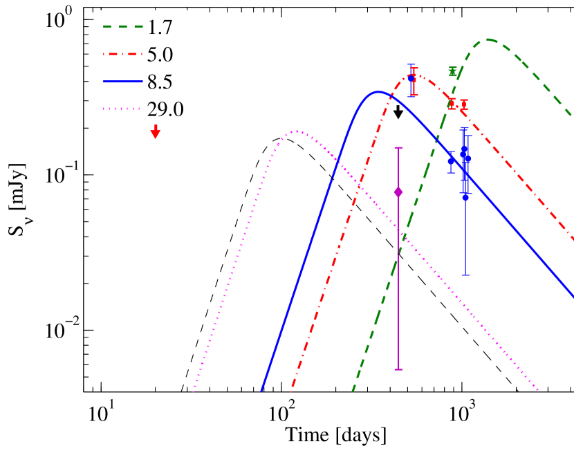
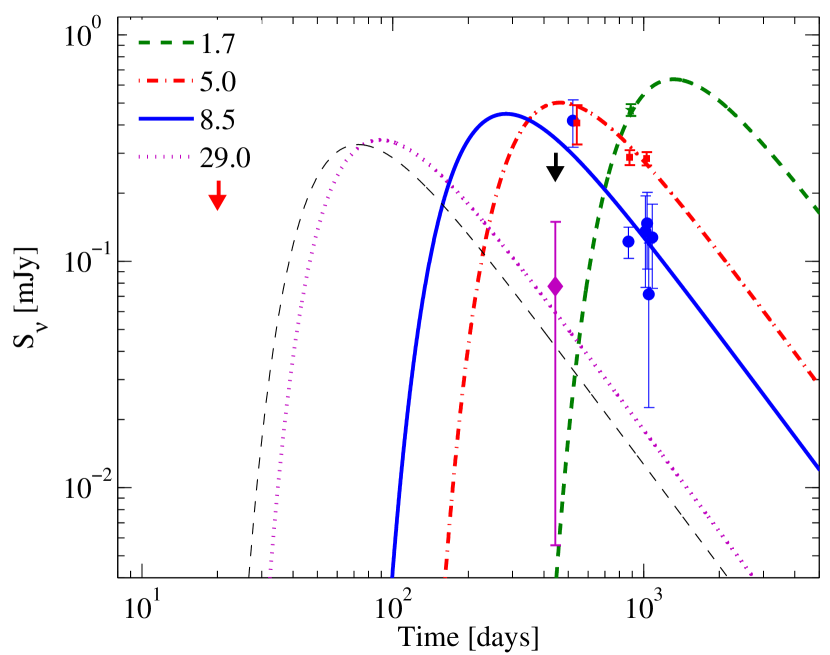
Figure 3: Parametrised radio light curve of SN 2010P –3 pure SSA and 3 pure FFA– at 1.7 GHz (green star, dashed line), 5.0 GHz (red squares, dash-dotted line), 8.5 GHz (blue circles, solid line) and 29 GHz (magenta diamond, dotted line). The downward arrows represent 3$\sigma$ upper limits from epochs E1 (red), and E3 (black). The black dashed line is the predicted light curve at 36.0 GHz.

Using the time dependence of the absorption due to the ionized CSM, the deceleration parameter is calculated as $m=-\delta/3$, resulting in $0.74\pm 0.01$ for SN 2010P. In the FFA case at peak times, if assuming that the ejecta velocity can be measured from optical lines (e.g., H$\alpha$) 45 days after explosion (Weiler et al., 1986), we have that

$$R_{\mathrm{shell}}=\frac{3.89\mbox{$\times 10^{{1}{5}}$}}{m}\left(\frac{v_{\mathrm{shock}}}{1\mbox{$\times 10^{{4}}$}\,\,\mbox{$\mathrm{km\,s^{-1}}$}{}}\right)\left(\frac{t_{\mathrm{peak}}}{45\,\mathrm{days}}\right)^{m}\mathrm{cm}.$$

SN ejecta is expected to have a distribution in velocity as it moves through the CSM. For example, for the Type IIb SN 2011hs, $v_{\mathrm{shock}}$ ranged from 8,000 to 12,000  $\mathrm{km\,s^{-1}}$ (Bufano et al., 2014). Recently, Inserra et al. (2013) investigated the photometric properties of a group of moderately luminous Type II SNe and found that in the early phases of the SN explosion, the expansion velocities as measured from H$\alpha$ and H$\beta$, range between $10,000$–$12,000$  $\mathrm{km\,s^{-1}}$. For SN 2010P we use the commonly used shock velocity value for Type II SNe $v_{\mathrm{shock}}\approx 10,000$  $\mathrm{km\,s^{-1}}$ near maximum light (e.g., Weiler et al., 2002), as we lack measured shock velocity values (Paper I). Using the $m$ value we estimated above and the $t_{\mathrm{peak}}$ values from Table 6, we obtain $R_{\mathrm{shell}}=(29.6,20.3)\mbox{$\times 10^{{1}{5}}$}$ cm for $\nu_{\mathrm{peak}}=$ 5.0 and 8.5 GHz, respectively. These sizes do not violate the EVN limit of 4.3$\times 10^{{1}{7}}$ cm, and imply brightness temperatures of (3.2, 2.1)$\times 10^{{9}}$ K, and thus below the ICC limit. As we did in the SSA model, the average expansion speeds in this case are 7,380–8,410  $\mathrm{km\,s^{-1}}$ (or 0.02–0.03$c$), hence, also sub-relativistic.

To estimate the progenitor’s average mass-loss rate, we can follow two approaches. For the first approach, we consider equation (11) in Weiler et al. (2002) and we assume that only the uniform component of the CSM contributes to the absorption of SN 2010P radio emission, so that at day $t_{\mathrm{peak}}$, the ratio of $\dot{M}$ to $v_{\mathrm{wind10}}$ is given by

$$\frac{\dot{M}}{v_{\mathrm{wind10}}} = 3\mbox{$\times 10^{{-}{6}}$}~{}\langle\tau_{\mathrm{eff}}^{0.5}\rangle~{}m^{-1.5}~{}\left(\frac{v_{\mathrm{shock}}}{10^{4}\,\,\mbox{$\mathrm{km\,s^{-1}}$}}\right)^{1.5}$$

$$\times \left(\frac{t_{\mathrm{peak}}}{45\,\mathrm{days}}\right)^{1.5m}\left(\frac{T}{10^{4}\,\mathrm{K}}\right)^{0.68}$$

with $\langle\tau_{\mathrm{eff}}^{0.5}\rangle=\tau_{\mathrm{external}}^{0.5}$, which for SN 2010P is $\sim 0.82$ at all the considered frequencies. Assuming that $v_{\mathrm{shock}}\approx 10,000$  $\mathrm{km\,s^{-1}}$, and 10,000 K for the CSM temperature $T$ (corresponding to the equilibrium temperature of a typical HII region), we obtain $\dot{M}/v_{\mathrm{wind10}}=(5.1,3.0)\mbox{$\times 10^{{-}{5}}$}$ at 5.0 and 8.5 GHz, respectively.

Alternatively, a second approach would be to follow Weiler et al.’s equation (18) for Type II SNe at 5 GHz:

$$\frac{\dot{M}}{v_{\mathrm{wind10}}}=1\mbox{$\times 10^{{-}{6}}$}\left(\frac{L_{\mathrm{peak}}}{10^{26}\,\,\mathrm{erg\,s^{-1}\,Hz^{-1}}{}}\right)^{0.54}\left(\frac{t_{\mathrm{peak}}}{\mathrm{days}}\right)^{0.38}$$

we obtain $\dot{M}/v_{\mathrm{wind10}}<4.0\mbox{$\times 10^{{-}{5}}$}$, consistent with the upper limit obtained following the first approach. We note that the relation used as a second approach does not depend on $v_{\mathrm{shock}}$ and thus, assuming that $\dot{M}/v_{\mathrm{wind10}}$ is equally good following the first and the second approach, we can plug in the ratio obtained here at 5 GHz into the first relation to solve for $v_{\mathrm{shock}}$. We obtain $v_{\mathrm{shock}}\sim 8,400$  $\mathrm{km\,s^{-1}}$ at 5 GHz, which matches quite well with the average expansion speed we estimated above. From now on, we consider $\dot{M}/v_{\mathrm{wind10}}=(3.0$–5.1)$\times 10^{{-}{5}}$ as a representative value for the mass-loss rate to wind velocity ratio.

We can now also estimate the CSM density as

$$\rho_{\mathrm{CSM}} = 1.6\mbox{$\times 10^{{6}}$}\left(\frac{\dot{M}}{1\mbox{$\times 10^{{-}{5}}$}\,\mbox{$\mathrm{M_{\sun}\,yr^{-1}}$}{}}\right)\left(\frac{v_{\mathrm{wind}}}{10\,\,\mbox{$\mathrm{km\,s^{-1}}$}{}}\right)^{-1}$$

$$\times \left(\frac{R_{\mathrm{shell}}}{1\mbox{$\times 10^{{1}{5}}$}\mathrm{cm}}\right)^{-2}~{}\mathrm{g~{}cm}^{-3}$$

(e.g., Horesh et al., 2013). For SN 2010P, this leads to $\rho_{\mathrm{CSM}}=$ (0.7, 1.2)$\times 10^{{4}}$ g cm^-3 at 5.0 and 8.5 GHz, respectively.

Table 6: Approximate peak values from the pure FFA fit.

Frequency	$t_{\mathrm{peak}}$	$S_{\mathrm{peak}}$	$L_{\mathrm{peak}}$
(GHz)	(days)	( $\mathrm{\mu Jy}$)	($\,\mathrm{erg\,s^{-1}\,Hz^{-1}}$)
1.7	1307	637	1.5$\times 10^{{2}{7}}$
5.0	464	502	1.2$\times 10^{{2}{7}}$
8.5	280	448	1.1$\times 10^{{2}{7}}$
29.0	88	343	8.2$\times 10^{{2}{6}}$

3.3.3 FFA vs. SSA

In Sections 3.3.1 and 3.3.2 we have obtained physical parameters for SN 2010P assuming pure SSA and pure FFA models dominating its radio emission.

The reduced $\chi^{2}$ of the SSA model doubles that of the FFA model, indicating that FFA describes better the late-time observations we present here. Beyond this, we also note some inconsistencies in the inferred parameters from the SSA model. For instance, following two different approaches we found that the deceleration parameter is $\ga 1$ in the pure SSA model. This clashes with the expectation of rapid deceleration as the SN shock moves into a dense CSM, and implies that the blast wave has been expanding at average shock velocities $<2,700\,\,\mbox{$\mathrm{km\,s^{-1}}$}$ (Section 3.3.1). These velocities are unrealistically low, whereas those obtained for FFA are in fact physically reliable and agree better with measured velocities for other SNe (Inserra et al., 2013) (see Section 3.3.2). Furthermore, the low mass-loss to wind velocity ratio we obtained in the pure SSA model ($\dot{M}[\,\mbox{$\mathrm{M_{\sun}\,yr^{-1}}$}{}]/v_{\mathrm{wind}}[10\,\,\mbox{$\mathrm{km\,s^{-1}}$}{}]=$(1.6–1.9)$\times 10^{{-}{7}}$), is difficult to reconcile with the high luminosity of SN 2010P.

Whilst SSA might be important at early stages of SN 2010P (where the existing data is scarce), we find that the FFA model fits the available data better and we thus adopt FFA as the dominant absorption mechanism for SN 2010P.

3.3.4 SN 2010P characterisation and radio parameters

In Table 7 we show the fitting parameters for SN 2010P we obtained when assuming FFA (Section 3.3.2), together with those of other well-studied Type II radio SNe from the literature for comparison purposes. We only included those fitting parameters relevant for comparison with SN 2010P.

From Table 7 we note that Type IIb SNe have the steepest spectral indices among the Type II SNe, as well as the lowest mass-loss rates, and this is the case as well for SN 2010P. Other parameters such as $K_{1}$ and $\beta$ vary greatly among SNe of the same type, thus cannot be used to set further constraints. The value for parameter $\delta$ tends to be smaller for Type IIL and IIn SNe, and the one we obtained for SN 2010P is typical for Type IIb SNe, with the exception of SN 2011hs, whose $\delta$ is significantly different from the value fitted for other Type IIb SNe, however, this is consistent with the rapid deceleration observed in the time evolution of the ejecta velocity (Bufano et al. 2014).

Parameter $K_{2}$ is indeed much larger for SN 2010P compared to other Type IIb SNe. However, we note that such a high value has also been obtained for SN 2001gd when assuming a pure FFA model for its radio light curve (Stockdale et al., 2003), as we have assumed for SN 2010P. Stockdale et al. (2007) improved on their results from 2003 by gathering a more complete data set of observations, and combining SSA and FFA components in the parametrization of the SN 2001gd light curves.

Table 7: Fitting parameters from radio light-curve models of SN 2010P and known Type II SNe.

SN	$\alpha$	$\beta$	$\delta$	$K_{1}$	$K_{2}$	$t_{\mathrm{peak}}$	$L_{\mathrm{peak}}$	$\dot{M}/v_{\mathrm{wind10}}$
				(mJy)		(days)	($\,\mathrm{erg\,s^{-1}\,Hz^{-1}}$)
2010P (IIb)a	$-1.62\pm 0.33$	$-1.49_{-0.05}^{+0.01}$	$-2.22_{-0.02}^{+0.02}$	$9.20_{-1.15}^{+4.12}\mbox{$\times 10^{{3}}$}$	$5.68_{-0.72}^{+0.98}\mbox{$\times 10^{{5}}$}$	$\sim 464$	$\sim 1.2\mbox{$\times 10^{{2}{7}}$}$	($3.0$–$5.1)\mbox{$\times 10^{{-}{5}}$}$
1993J (IIb)b	$-0.81$	$-0.73$	$-1.88$	$4.8\mbox{$\times 10^{{3}}$}$	$1.6\mbox{$\times 10^{{2}}$}$	133	$1.5\mbox{$\times 10^{{2}{7}}$}$	(0.5-5.9)$\times 10^{{-}{5}}$
2001gd (IIb)c	$-0.94$	$-0.92$	$-1.88$	$7.50\mbox{$\times 10^{{2}}$}$	$1.50\mbox{$\times 10^{{3}}$}$	80	$3.8\mbox{$\times 10^{{2}{7}}$}$	$(0.7-5.6)\mbox{$\times 10^{{-}{5}}$}$
2001ig (IIb)d	$-1.06$	$-1.50$	$-2.56$	$2.71\mbox{$\times 10^{{4}}$}$	$1.38\mbox{$\times 10^{{3}}$}$	74	$3.5\mbox{$\times 10^{{2}{7}}$}$	$(2.2\pm 0.5)\mbox{$\times 10^{{-}{5}}$}$
2011hs (IIb)e	$-1.90$	$-1.66$	$-1.31$	$5.2\mbox{$\times 10^{{3}}$}$	$1.5\mbox{$\times 10^{{2}}$}$	59	$1.6\mbox{$\times 10^{{2}{7}}$}$	$(2.0\pm 0.6)\mbox{$\times 10^{{-}{5}}$}$
1970G (IIL)f	$-0.55$	$-1.87$	$-3.00$	$1.77\mbox{$\times 10^{{6}}$}$	$1.80\mbox{$\times 10^{{7}}$}$	307	$1.4\mbox{$\times 10^{{2}{7}}$}$	$6.8\mbox{$\times 10^{{-}{5}}$}$
1979C (IIL)f	$-0.75$	$-0.80$	$-2.94$	$1.72\mbox{$\times 10^{{3}}$}$	$3.38\mbox{$\times 10^{{7}}$}$	556	$2.6\mbox{$\times 10^{{2}{7}}$}$	$1.1\mbox{$\times 10^{{-}{4}}$}$
1980K (IIL)f	$-0.60$	$-0.73$	$-2.69$	$1.15\mbox{$\times 10^{{2}}$}$	$1.42\mbox{$\times 10^{{5}}$}$	134	$1.2\mbox{$\times 10^{{2}{6}}$}$	$1.3\mbox{$\times 10^{{-}{5}}$}$
1978K (IIn)g	$-0.77$	$-1.55$	$-2.22$	(0.2-76)$\times 10^{{7}}$	(0.3-90)$\times 10^{{4}}$	940-1000	(0.9-2.0)$\times 10^{{2}{8}}$	$1.0\mbox{$\times 10^{{-}{4}}$}$
1986J (IIn)f	$-0.66$	$-1.65$	-	$1.19\mbox{$\times 10^{{7}}$}$	-	1210	$2.0\mbox{$\times 10^{{2}{8}}$}$	$4.3\mbox{$\times 10^{{-}{5}}$}$
1988Z (IIn)f	$-0.69$	$-1.25$	-	$1.47\mbox{$\times 10^{{4}}$}$	-	898	$2.3\mbox{$\times 10^{{2}{8}}$}$	$1.1\mbox{$\times 10^{{-}{4}}$}$
2000ft (IIn)h	$-1.27$	$-2.02$	$-2.94$	$4.45\mbox{$\times 10^{{5}}$}$	$1.67\mbox{$\times 10^{{7}}$}$	300	$1.1\mbox{$\times 10^{{2}{8}}$}$	(4.7-5.1)$\times 10^{{-}{5}}$

This is not a complete list of fitting parameters. References: (a) This work, (b) Weiler et al. 2007, (c) Stockdale et al. 2007, (d) Ryder et al. 2004, (e) Bufano et al. 2014, (f) Weiler et al. 2002, (g) Schlegel et al. 1999, (h) Pérez-Torres et al. 2009a.

The fitted light curves we present in Figure 3 assuming FFA, reproduce the optically thin behaviour we infer from our spectral index measurements at 2.4 and 2.8 yr (see Figure 2), and provide a rough estimate for the time it took the SN to reach its peak at 5 GHz ($t_{\mathrm{peak}}\sim 464$ days) and the corresponding peak luminosity at 5 GHz ($L_{\mathrm{peak}}\sim 1.2\mbox{$\times 10^{{2}{7}}$}$$\,\mathrm{erg\,s^{-1}\,Hz^{-1}}$), which can be used to infer the SN type (see Figure 4). We note that SN 2010P lies close to Type IIL SNe in that plot. However, the early optical spectrum of SN 2010P (Paper I) does not show strong hydrogen features, as should be observed in a typical Type IIL SN.

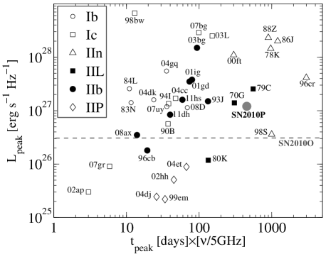
Figure 4: Peak monochromatic luminosity vs. time to peak from explosion date for different types of CCSNe (hypernovae and other peculiar objects included). The first peak is used in case more than one has been reported. The dashed line represents the upper limit in luminosity for SN 2010O. References: Weiler et al. (2002) for SNe 1970G, 1979C, 1980K, 1983N, 1984L, 1986J, 1988Z, 1990B and 1994I; Pooley et al. (2002) for 1998S and 1999em; Wellons, Soderberg, & Chevalier (2012) for 2004cc, 2004dk and 2004gq; van der Horst et al. (2011) for 2007uy and 2008D; Schlegel et al. (1999) for 1978K; Weiler et al. (2007) for 1993J; Weiler et al. (1998) for 1996cb; Bauer et al. (2008) for 1996cr; Weiler, Panagia, & Montes (2001) for 1998bw; Pérez-Torres et al. (2009a) for 2000ft; Stockdale et al. (2007) for 2001gd; Ryder et al. (2004) for 2001ig; Berger, Kulkarni, & Chevalier (2002) for 2002ap; Chevalier, Fransson, & Nymark (2006) for 2002hh; Soderberg et al. (2005) for 2003L; Soderberg et al. (2006) for 2003bg; Beswick et al. (2005) for 2004dj; Martí-Vidal et al. (2007) for 2004et; Salas et al. (2013) for 2007bg; Soderberg et al. (2010) for 2007gr; Roming et al. (2009) for 2008ax; Maeda (2012) for 2011dh (see also Horesh et al., 2013); Bufano et al. (2014) for 2011hs.

4 Discussion

The optical spectroscopy reported in Paper I indicates that 2010O is a Type Ib SN, which are known to be bright at radio frequencies. In fact a peak luminosity $<3\mbox{$\times 10^{{2}{6}}$}$ $\,\mathrm{erg\,s^{-1}\,Hz^{-1}}$ (see Figure 4) is quite uncommon for Type Ib/c SNe (Soderberg, 2007). Additionally, these SNe evolve very rapidly and thus reach their peak luminosity within a few tens of days (e.g., SN 2008D, Soderberg et al., 2008), so the most likely explanation for the radio non-detection of SN 2010O is that it reached its peak some time after the early-time MERLIN observations by Beswick et al., and well before our observations in 2011, so it went unnoticed owing to the lack of prompt radio observations.

SN 2010P lies in a location with larger extinction than seen toward SN 2010O ($A_{V}=7$ mag, Paper I) and at a $\approx 160$ pc projected distance from the component C^′, SN 2010P is the first radio SN detected in the outskirts of a bright radio emitting component in Arp 299, despite the intense radio monitoring. Its strong radio emission 1.4 to 2.8 yr after explosion indicates a strong interaction between the SN ejecta and the CSM. Whilst the early optical spectrum is consistent with the SN being either a Type Ib or IIb (Paper I), the late-time radio detection rules out a Type Ib origin.

The parameters we obtained to fit the radio light curve of SN 2010P are common for luminous Type II SNe (see Table 7). Whilst the inferred peak luminosity and the time to reach the peak are more comparable to those of Type IIL’s, its estimated mass-loss rate to wind velocity ratio, $\dot{M}/v_{\mathrm{wind10}}=(3.0$–$5.1)\mbox{$\times 10^{{-}{5}}$}$, and its inferred deceleration parameter ($\sim 0.74$), support better a Type IIb nature with a slow evolution, and are consistent with the early optical spectra lacking strong hydrogen features (Paper I). We note that some Type IIn SNe have comparable mass-loss rate to wind velocity ratios (see Table 7), however, these SNe are also an order of magnitude more luminous than SN 2010P at their peak.

It has been suggested that Type IIb SNe can be divided into two broad groups (Chevalier & Soderberg, 2010) under the assumption that SSA is the main absorption mechanism: i) slowly evolving SNe at radio frequencies ($t_{\mathrm{peak}}>100$ d) with a large ($>0.1\,\,\mbox{$\mathrm{M_{\sun}}$}{}$) hydrogen mass envelope and slow ejecta velocity ($\sim 10,000\,\,\mbox{$\mathrm{km\,s^{-1}}$}{}$), expected from an extended progenitor ($R\sim 10^{13}$ cm); ii) rapidly evolving SNe ($t_{\mathrm{peak}}<100$ d) with a small hydrogen mass envelope ($<0.1\,\,\mbox{$\mathrm{M_{\sun}}$}{}$) and fast ejecta velocities (a factor of 3-5 larger than in case i), expected from a compact progenitor ($R\sim 10^{11}$ cm). According to this interpretation, SN 2010P would come from an extended progenitor since it took hundreds of days to reach its peak (in both FFA and SSA fits). In Paper I we do not find evidence for a large hydrogen mass envelope (i.e., $>0.1\,\,\mbox{$\mathrm{M_{\sun}}$}{}$) around SN 2010P, in contradiction with the expectations for an extended progenitor as inferred from its radio behaviour. The properties of SNe 2011dh and 2011hs where more direct evidence of the progenitor star has been obtained (Bersten et al., 2012; Bufano et al., 2014, respectively), further suggest that the inferred radio properties of a SN are not a strong beacon of the progenitor size. This could be related to the assumption of SSA dominance for poorly sampled light curves.

In the case of SN 2001gd, the assumptions made to fit its radio light curve greatly affected the estimate for the time it took the SN to reach its peak at 5 GHz, going from 173 d in the FFA model (Stockdale et al., 2003), to 80 d in the SSA$+$FFA model (Stockdale et al., 2007), thus placing this SN in the compact IIb category, following the interpretation from Chevalier & Soderberg (2010). Unlike in the SN 2001gd case, we do not have early data for SN 2010P describing its turn-on phase at any frequency, and thus, we cannot quantify the presence of SSA in its evolution. However, it is rather unlikely that SSA will dominate the absorption for SN 2010P radio emission when the SN has been detected at such late ages. Thus, although the $t_{\mathrm{peak}}{}$ we estimated for SN 2010P represents an upper limit owing to our assumption of FFA being the only absorption mechanism, we have seen that assuming an SSA model pushes the peak at different frequencies to even later times and the same interpretation holds.

However, there is another possible scenario which we cannot exclude. SN 2010P could have reached a first peak at early times not sampled by our data, and we could in fact be witnessing a re-brightening of the SN at later times. In this situation, $t_{\mathrm{peak}}$ would have occurred earlier and SN 2010P would appear closer to other Type IIb SNe in the $L_{\mathrm{peak}}$ vs. $t_{\mathrm{peak}}$ plot.

Observationally, strong variations in the optically thin phase of different types of CCSNe are rather common (see table 4 in Soderberg et al., 2006) owing to the complexity of their CSM. For Type IIb SNe, it has been shown that variations in the mass-loss of the progenitor (e.g., luminous blue variable-like stars), can create inhomogeneities in the CSM and thus modulations in the SN radio light curve (e.g., Kotak & Vink, 2006; Moriya, Groh, & Meynet, 2013).

The sparse sampling of the SN 2010P light curve does not allow us to conclusively determine whether our late-time observations match with the forward shock encountering a first, or a second high-density region. Multiple high-density regions can be produced by mass-loss episodes, meaning variations in the mass-loss rate throughout the lifetime of the progenitor star. However, the early optical/NIR data (Paper I) do not show evidence for interaction with the CSM at the early stages of the SN, i.e., the interaction with the CSM corresponding to the end of the progenitor star’s lifetime. Therefore, although we cannot rule out completely the possibility of the peak radio luminosity corresponding to a secondary mass-loss episode, the observations (both radio and NIR) strongly suggest that we are witnessing a slow radio evolution of SN 2010P.

5 Conclusions

We report radio observations towards SNe 2010O and 2010P in the LIRG Arp 299. SN 2010O was not detected throughout our radio monitoring of the host galaxy which lacked observations of the SN at ages between 0.6 month and 1.4 yr, time enough for a Type Ib SN to have have risen to a peak, then decayed. SN 2010P was detected at various frequencies in its transition to, and in its optically thin phase from $\sim$1 to $\sim$3 yr after explosion. Our observations favour FFA as the dominant absorption mechanism controlling the radio emission of this SN. We characterise it as a luminous, slowly-evolving Type IIb SN with $\dot{M}[\,\mbox{$\mathrm{M_{\sun}\,yr^{-1}}$}{}]/v_{\mathrm{wind}}[10\,\,\mbox{$\mathrm{km\,s^{-1}}$}{}]=(3.0$–5.1)$\times 10^{{-}{5}}$. We have also improved on the coordinates previously reported for SN 2010P with a position accuracy better than 1 mas at $\alpha(J2000)=11\mathrm{{}^{h}}28\mathrm{{}^{m}}31\aas@@fstack{s}3605$, $\delta(J2000)=58\degr 33\arcmin 49\aas@@fstack{\prime\prime}315$.

SN 2010P is one of a select group of 12 Type IIb SNe detected at radio wavelengths: for nine of them a radio light curve has been obtained (see references in Figure 4), and three of them have only reported radio detections (SNe 2008bo, PTF 12os and 2013ak reported in Stockdale et al., 2008, 2012; Kamble et al., 2014, respectively).

SN 2010P is also the most distant Type IIb SN detected so far, and the one that according to our data, has taken the longest time to reach its peak. However, a comprehensive, multi-wavelength study covering both rise and decline of the SN emission is needed to investigate possible progenitor star scenarios. We note that the early epochs after shock breakout are crucial, since this when when we can gather more information about the progenitors and the dominant absorption mechanism (SSA/FFA) shaping the radio light curves, thus helping us to better understand the CCSN phenomenon, and thereby the interplay between massive stars and their CSM.

Appendix A Radio light-curve fit

We performed a Monte Carlo optimization to obtain a robust fit for the radio light curves of SN 2010P. We generated 10,000 random flux densities for each observing epoch with a detection, assuming that these follow a normal distribution with mean $S_{\nu}$ and standard deviation $\sigma$ (from Table 4). The random flux densities were restricted to positive values within the interval $-2\sigma$ to $+2\sigma$, thus covering the $95.4$ per cent of each epoch flux density distribution.

We then created 10,000 sets (each composed of one flux value per epoch) to which we applied a non-linear least-squares regression method within MATLAB (from MathWorks). This process yielded a normal distribution for $K_{1}$, $K_{5}$, $\beta$ and $\delta^{\prime\prime}$ in the pure SSA model as shown in Figure 5, and for $K_{1}$, $K_{2}$, $\beta$ and $\delta$ in the pure FFA model as shown in Figure 6. For each distribution, i.e., for each parameter, the mean value is determined by the intersection of the solid line at $0.5$ with the curve, and the intersection with the dashed lines at $0.16$ and $0.84$ are the $-1\sigma$ and $+1\sigma$ values, respectively.

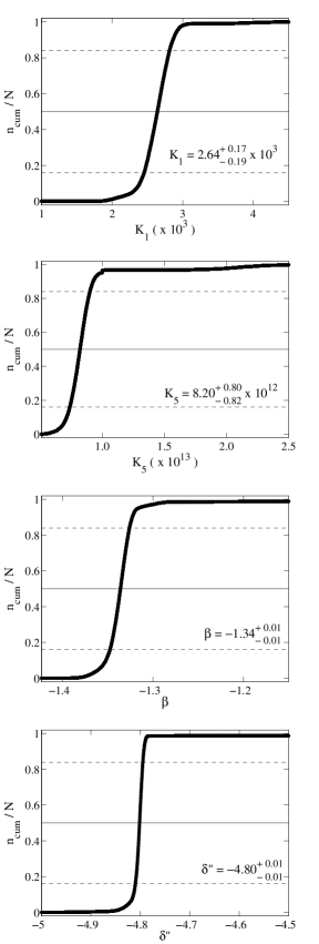
Figure 5: Normalised cumulative distribution of the fitting parameters in the pure SSA model. The solid line represents the mean and the dashed lines represent $-1\sigma$ and $+1\sigma$ of the distribution, repectively.

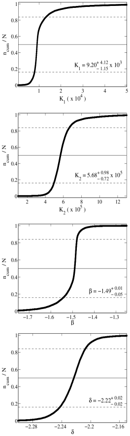
Figure 6: Normalised cumulative distribution of the fitting parameters in the pure FFA model. Solid and dashed lines are as described in Figure 5.

A.1 Pure SSA fit parameters

The cumulative distributions for $K_{1}$, $K_{5}$, $\beta$ and $\delta^{\prime\prime}$, whilst consistent with a Gaussian distribution, show some departures from the expected behaviour, as they reach a value of unity very abruptly. We note that the high value of $K_{5}$ implies that the SSA absorption is very important; however, the high negative value of $\delta^{\prime\prime}$ indicates that the absorption decreases quite quickly with time, and tells us that SSA is more important at early stages in the evolution SN 2010P. Thus, the poor sampling we have on the optically thick part of the radio light curves, inevitably results in a poor SSA fit.

A.2 Pure FFA fit parameters

Parameter $K_{1}$ is the least symmetric in its cumulative distribution, however, it still resembles a Gaussian shape. The available number of epochs with detections at each frequency is not sufficient to constrain further parameters such as $K_{3}$ and $K_{4}$, and we therefore assumed them to be negligible. In Table 8 we compare the values for $K_{3}$ and $K_{4}$ fitted for known Type II SNe and SN 2010P. In most cases the term $K_{4}$ is absent, meaning that a putative distant ionized gas is not affecting the expansion of the SN ejecta. Thus, considering $K4\sim 0$ for SN 2010P is a fair assumption.

In the case of $K_{3}$, we note however that when included in the fit of other SNe, it takes significantly high values. To explore its possible influence on the fit, we investigate the $A_{2}$ term in Equation 1. $A_{2}$ takes values between 0 and 1, and for it to have some effect on the light-curve fitting requires that $0.01\la\tau_{\mathrm{CSM}_{\mathrm{clumps}}}\la 100$ (see Figure 7). This implies that a meaningful $K_{3}$ would take the following values at each of the frequencies we present data for: $6\mbox{$\times 10^{{6}}$}\la K_{3}\la 2\mbox{$\times 10^{{1}{2}}$}$, $6\mbox{$\times 10^{{7}}$}\la K_{3}\la 2\mbox{$\times 10^{{1}{3}}$}$, $2\mbox{$\times 10^{{8}}$}\la K_{3}\la 5\mbox{$\times 10^{{1}{3}}$}$ and $3\mbox{$\times 10^{{9}}$}\la K_{3}\la 7\mbox{$\times 10^{{1}{4}}$}$ at 5.0 and 8.5 GHz, respectively. Therefore, $K_{3}<6\mbox{$\times 10^{{6}}$}$ would have the same effect as $K_{3}\sim 0$ at all the frequencies considered here. We cannot set strong constraints on $K_{3}$ owing to our sparse sampling at each frequency, and we note that the presence of a clumpy absorbing medium is not needed to reproduce the spectral behaviour of SN 2010P. Thus, we assume $K_{3}\sim 0$.

Table 8: Absorption terms $K_{3}$ and $K_{4}$ from radio light-curve models of SN 2010P and known Type II SNe.

SN	$K_{3}$	$K_{4}$
2010P (IIb)a	0.0	0.0
1993J (IIb)b	$4.6\mbox{$\times 10^{{5}}$}$	0.0
2001gd (IIb)c	-	-
2001ig (IIb)d	$1.47\mbox{$\times 10^{{5}}$}$	0.0
2011hs (IIb)e	$1.9\mbox{$\times 10^{{5}}$}$	0.0
1970G (IIL)f	-	-
1979C (IIL)f	-	-
1980K (IIL)f	-	-
1978K (IIn)g	(0.03-30)$\times 10^{{1}{1}}$	$9\mbox{$\times 10^{{-}{3}}$}$
1986J (IIn)f	$3.06\mbox{$\times 10^{{9}}$}$	-
1988Z (IIn)f	$5.39\mbox{$\times 10^{{8}}$}$	0.0
2000ft (IIn)h	-	$\ga 0.17$

The references are those from Table 7.

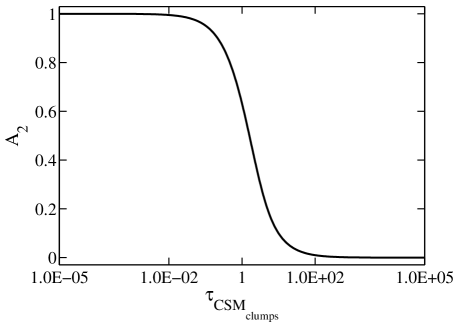
Figure 7: Behaviour of the absorption by a clumpy medium.

References

- Alonso-Herrero et al. (2000) Alonso-Herrero A., Rieke G. H., Rieke M. J., Scoville N. Z., 2000, ApJ, 532, 845
- Anderson, Habergham, & James (2011) Anderson J. P., Habergham S. M., James P. A., 2011, MNRAS, 416, 567
- Bauer et al. (2008) Bauer F. E., Dwarkadas V. V., Brandt W. N., Immler S., Smartt S., Bartel N., Bietenholz M. F., 2008, ApJ, 688, 1210
- Berger, Kulkarni, & Chevalier (2002) Berger E., Kulkarni S. R., Chevalier R. A., 2002, ApJ, 577, L5
- Bersten et al. (2012) Bersten M. C., et al., 2012, ApJ, 757, 31
- Beswick et al. (2005) Beswick R. J., Muxlow T. W. B., Argo M. K., Pedlar A., Marcaide J. M., Wills K. A., 2005, ApJ, 623, L21
- Beswick et al. (2010) Beswick R. J., Perez-Torres M. A., Mattila S., Garrington S. T., Kankare E., Ryder S., Alberdi A., Romero-Canizales C., 2010, ATel, 2432, 1
- Bondi et al. (2012) Bondi M., Pérez-Torres M. A., Herrero-Illana R., Alberdi A., 2012, A&A, 539, A134
- Brunthaler et al. (2009) Brunthaler A., Menten K. M., Reid M. J., Henkel C., Bower G. C., Falcke H., 2009, ATel, 2020, 1
- Bufano et al. (2014) Bufano F., et al., 2014, MNRAS, 224
- Chevalier (1982) Chevalier R. A., 1982, ApJ, 259, 302
- Chevalier (1998) Chevalier R. A., 1998, ApJ, 499, 810
- Chevalier, Fransson, & Nymark (2006) Chevalier R. A., Fransson C., Nymark T. K., 2006, ApJ, 641, 1029
- Chevalier & Soderberg (2010) Chevalier R. A., Soderberg A. M., 2010, ApJ, 711, L40
- Gehrz, Sramek, & Weedman (1983) Gehrz R. D., Sramek R. A., Weedman D. W., 1983, ApJ, 267, 551
- Herrero-Illana et al. (2012) Herrero-Illana R., Romero-Canizales C., Perez-Torres M. A., Alberdi A., Kankare E., Mattila S., Ryder S. D., 2012, ATel, 4432, 1
- Horesh et al. (2013) Horesh A., et al., 2013, MNRAS, 2312
- Inserra et al. (2013) Inserra C., et al., 2013, A&A, 555, A142
- Kamble et al. (2014) Kamble A., Soderberg A., Zauderer B. A., Chakraborti S., Margutti R., Milisavljevic D., 2014, ATel, 5763, 1
- Kankare et al. (2008) Kankare E., et al., 2008, ApJ, 689, L97
- Paper I (2013) Kankare E., et al., 2013, MNRAS, 2968
- Kotak & Vink (2006) Kotak R., Vink J. S., 2006, A&A, 460, L5
- Krauss et al. (2012) Krauss M. I., et al., 2012, ApJ, 750, L40
- Leroy et al. (2011) Leroy A. K., et al., 2011, ApJ, 739, L25
- Maeda (2012) Maeda K., 2012, ApJ, 758, 81
- Magnelli et al. (2011) Magnelli B., Elbaz D., Chary R. R., Dickinson M., Le Borgne D., Frayer D. T., Willmer C. N. A., 2011, A&A, 528, A35
- Martí-Vidal et al. (2007) Martí-Vidal I., et al., 2007, A&A, 470, 1071
- Mattila et al. (2007) Mattila S., et al., 2007, ApJ, 659, L9
- Mattila & Kankare (2010) Mattila S., Kankare E., 2010, CBET, 2145, 1
- Mattila et al. (2010) Mattila S., Kankare E., Datson J., Pastorello A., 2010, CBET, 2149, 1
- Mattila et al. (2012) Mattila S., et al., 2012, ApJ, 756, 111
- Mattila et al. (2013) Mattila S., Fraser M., Smartt S. J., Meikle W. P. S., Romero-Cañizales C., Crockett R. M., Stephens A., 2013, MNRAS, 431, 2050
- McMullin et al. (2007) McMullin J. P., Waters B., Schiebel D., Young W., Golap K., 2007, ASPC, 376, 127
- Moriya, Groh, & Meynet (2013) Moriya T. J., Groh J. H., Meynet G., 2013, A&A, 557, L2
- Neff, Ulvestad, & Teng (2004) Neff S. G., Ulvestad J. S., Teng S. H., 2004, ApJ, 611, 186
- Nelemans et al. (2010) Nelemans G., Voss R., Nielsen M. T. B., Roelofs G., 2010, MNRAS, 405, L71
- Newton, Puckett, & Orff (2010) Newton J., Puckett T., Orff T., 2010, CBET, 2144, 2
- Pérez-Torres et al. (2009a) Pérez-Torres M. A., Alberdi A., Colina L., Torrelles J. M., Panagia N., Wilson A., Kankare E., Mattila S., 2009a, MNRAS, 399, 1641
- Pérez-Torres et al. (2007) Pérez-Torres M. A., et al., 2007, ApJ, 671, L21
- Pérez-Torres et al. (2009b) Pérez-Torres M. A., Romero-Cañizales C., Alberdi A., Polatidis A., 2009b, A&A, 507, L17
- Pooley et al. (2002) Pooley D., et al., 2002, ApJ, 572, 932
- Readhead (1994) Readhead A. C. S., 1994, ApJ, 426, 51
- Romero-Cañizales et al. (2011) Romero-Cañizales C., Mattila S., Alberdi A., Pérez-Torres M. A., Kankare E., Ryder S. D., 2011, MNRAS, 415, 2688
- Roming et al. (2009) Roming P. W. A., et al., 2009, ApJ, 704, L118
- Ryder et al. (2010) Ryder S., Mattila S., Kankare E., Perez-Torres M., 2010, CBET, 2189, 1
- Ryder et al. (2004) Ryder S. D., Sadler E. M., Subrahmanyan R., Weiler K. W., Panagia N., Stockdale C., 2004, MNRAS, 349, 1093
- Salas et al. (2013) Salas P., Bauer F. E., Stockdale C., Prieto J. L., 2013, MNRAS, 428, 1207
- Sanders et al. (2003) Sanders D. B., Mazzarella J. M., Kim D.-C., Surace J. A., Soifer B. T., 2003, AJ, 126, 1607
- Schlegel et al. (1999) Schlegel E. M., Ryder S., Staveley-Smith L., Petre R., Colbert E., Dopita M., Campbell-Wilson D., 1999, AJ, 118, 2689
- Shepherd, Pearson, & Taylor (1995) Shepherd M. C., Pearson T. J., Taylor G. B., 1995, BAAS, 27, 903
- Soderberg (2007) Soderberg A. M., 2007, AIPC, 937, 492
- Soderberg et al. (2008) Soderberg A. M., et al., 2008, Natur, 453, 469
- Soderberg et al. (2010) Soderberg A. M., Brunthaler A., Nakar E., Chevalier R. A., Bietenholz M. F., 2010, ApJ, 725, 922
- Soderberg et al. (2006) Soderberg A. M., Chevalier R. A., Kulkarni S. R., Frail D. A., 2006, ApJ, 651, 1005
- Soderberg et al. (2005) Soderberg A. M., Kulkarni S. R., Berger E., Chevalier R. A., Frail D. A., Fox D. B., Walker R. C., 2005, ApJ, 621, 908
- Stockdale et al. (2003) Stockdale C. J., Weiler K. W., Van Dyk S. D., Montes M. J., Panagia N., Sramek R. A., Perez-Torres M. A., Marcaide J. M., 2003, ApJ, 592, 900
- Stockdale et al. (2007) Stockdale C. J., Williams C. L., Weiler K. W., Panagia N., Sramek R. A., Van Dyk S. D., Kelley M. T., 2007, ApJ, 671, 689
- Stockdale et al. (2008) Stockdale C. J., Weiler K. W., Immler S., Marcaide J. M., Panagia N., van Dyk S. D., Sramek R. A., Pooley D., 2008, IAUC, 8939, 2
- Stockdale et al. (2012) Stockdale C. J., et al., 2012, ATel, 3882, 1
- Ulvestad (2009) Ulvestad J. S., 2009, AJ, 138, 1529
- van der Horst et al. (2011) van der Horst A. J., et al., 2011, ApJ, 726, 99
- Weiler et al. (1986) Weiler K. W., Sramek R. A., Panagia N., van der Hulst J. M., Salvati M., 1986, ApJ, 301, 790
- Weiler et al. (1998) Weiler K. W., van Dyk S. D., Montes M. J., Panagia N., Sramek R. A., 1998, ApJ, 500, 51
- Weiler, Panagia, & Montes (2001) Weiler K. W., Panagia N., Montes M. J., 2001, ApJ, 562, 670
- Weiler et al. (2002) Weiler K. W., Panagia N., Montes M. J., Sramek R. A., 2002, ARA&A, 40, 387
- Weiler et al. (2007) Weiler K. W., Williams C. L., Panagia N., Stockdale C. J., Kelley M. T., Sramek R. A., Van Dyk S. D., Marcaide J. M., 2007, ApJ, 671, 1959
- Wellons, Soderberg, & Chevalier (2012) Wellons S., Soderberg A. M., Chevalier R. A., 2012, ApJ, 752, 17