Abstract

Three classes of finite-dimensional models of quantum systems exhibiting spectral degeneracies called quantum catastrophes are described in detail. Computer-assisted symbolic manipulation techniques are shown unexpectedly efficient for the purpose.

Keywords

quantum theory; PT symmetry; finite-dimensional non-Hermitian Hamiltonians; exceptional-point localization; quantum theory of catastrophes; methods of computer algebra;

1 Introduction

For non-specialists, the presentation of some of the key ideas of quantum theory may be mediated by the technically next-to-trivial toy-model quantum systems ${\cal S}_{(N=2)}$ in which the representation of a dynamical state, i.e., in the Dirac’s notation, of the ket-vector element $|\psi^{(P)}\rangle$ of a pre-selected physical Hilbert space ${\cal H}^{(P)}$ is just a two-component complex vector

$$|\psi^{(P)}_{(N=2)}\rangle=\left(\begin{array}[]{c}\psi^{(P)}_{1}\\ \psi^{(P)}_{2}\end{array}\right)\,\in\,{\cal H}^{(P)}_{(N=2)}\,,\ \ \ \ \ {\cal H}^{(P)}_{(N=2)}\ \equiv\ \mathbb{C}^{2}\,.$$ (1)

Exaggerated as such a drastic reduction might seem, it still may be found in various analyses of the meaning and modern interpretations of quantum theory. In particular, precisely this simplification has been chosen by Dorey et al [1] as playing a crucial methodical role in the running development of the so called ${\cal PT}$-symmetric quantum mechanics (PTQM) in 2001.

One should remember that the ultimate formulation of PTQM theory was only completed a few years later (cf. [2, 3] and also [4] for more details). The key conceptual problems encountered during the introduction and development of the PTQM physics appeared difficult, albeit more or less purely technical. The work with $N-$dimensional analogues of Eq. (1) at suitable finite $N<\infty$ proved helpful.

Some of the problems emerged immediately after Bender and Boettcher [5] proposed, in 1998, a generalization of the usual description of the unitary evolution based on the current physical Schrödinger equation

$${\rm i}\partial_{t}\,|\psi^{(P)}\rangle=\mathfrak{h}\,|\psi^{(P)}\rangle\,$$ (2)

containing a Hermitian Hamiltonian $\mathfrak{h}=\mathfrak{h}^{\dagger}$. They declared that the explicit postulate of the Hermiticity of the Hamiltonian had to be weakened. Such an attempt opened the Pandora’s box of complicated mathematical questions, some of which remain unresolved up to these days (cf., e.g., [6]).

On positive side, the PTQM framework was found mathematically correct (it is briefly summarized in Appendix A below). Under suitable formal restrictions the formulation of which dates back to paper [7] by Scholtz et al in 1992, the potential applications of the theory do not even require any excessively complicated mathematics.

We intend to demonstrate that the PTQM formalism is exceptionally suitable for a computer-assisted model building. Having chosen a triplet of suitable $N$ by $N$ matrix examples (cf. their introduction in section 2) we shall present their detailed methodical analysis in a fully constructive and non-numerical, symbolic-manipulation-based spirit.

The key purpose of our message will lie in the demonstration of the not quite obvious feasibility of constructions at all dimensions. We shall assume that our Hamiltonians $H\neq H^{\dagger}$ can vary with one or more free parameters. This will open perspectives in analysis of less common quantum systems ${\cal S}$.

We shall consider the three series of $N$ by $N$ matrix models as initiated by the respective $N=2$ Hamiltonian matrices

$$\left[\begin{array}[]{cc}2-{\rm i}\lambda&-1\\ {}-1&2+{\rm i}\lambda\end{array}\right]\,,\ \ \ \left[\begin{array}[]{cc}2&-1+\lambda\\ {}-1-\lambda&\ 2\end{array}\right]\,,\ \ \ \left[\begin{array}[]{cc}2&-1+\lambda\\ {}-1-\lambda&\ 2\end{array}\right]\,$$ (3)

(notice that the second and the third items coincide at $N=2$). In all of these $N=2$ initial cases the determination of the bound state energies remains trivial yielding, incidentally, the same result,

$$E_{\pm}=2\pm\sqrt{1-\lambda^{2}}\,.$$

Surprisingly enough, we shall reveal that for all of our toy models, the facilitated tractability of spectra survives the generalizations $(N=2)\to(N>2)$. At any matrix dimension our examples will share the property of possessing a compact domain of acceptable physical parameters $\lambda\in{\cal D}$ at which the spectrum is real and non-degenerate. The $N>2$ descendants $H^{(N)}$ of the above three $N=2$ matrices will also share a number of further qualitative features. One of the important ones is that our Hamiltonians will cease to be diagonalizable at the boundary points of the respective domains ${\cal D}$. According to Kato [8], these boundary points may be called exceptional points (EP). We may also see that ${\cal D}=(-1,1)$ for $N=2$.

From the point of physics every EP manifold $\partial{\cal D}^{(N)}$ forms, in the space of parameters, a natural horizon of observability of the system. These horizons may intuitively be perceived as formal singularities alias instants of the physical system’s collapse. Depending on a more concrete interpretation of the system they may also carry the meaning of phase transition or of a cusp-like quantum catastrophe (QC, [9]). In section 3 we shall briefly return to this point and to the results of Ref. [9] which will be cited as paper I in what follows. These results will serve us as a methodical guide because, in particular, the underlying $N=2$ Hamiltonian

$$\left[\begin{array}[]{cc}1&\ \lambda\\ {}-\lambda&\ 3\end{array}\right]\,$$

might have very easily been added to the above list (3) as a fourth item.

In the rest of the paper we shall pay detailed attention to the new models and to the role of the computer-assisted symbolic manipulations in their analysis. In particular, in section 4 we shall sample the secular equations of the three new classes of $N$ by $N$ matrix models. As long as we will not impose restrictions on the size of dimension $N$, we shall argue that the computerized manipulations may be expected vital for the feasibility and success of the search for the parameters and spectra in the vicinity of the QC singularities.

In section 5 we shall re-attract the reader’s attention to an interplay between the topologically anomalous EP degeneracies of the spectra and certain geometrical features of the related physical Hilbert space. We shall explain how the computer-assisted manipulations can mediate or improve our insight into the mathematical structures of quantum systems which are close to the QC dynamical regime.

In the last section 6 a few comments on the purpose of our toy-model simulations and on the possible physics of quantum systems near QC will be added.

2 The QC menu of $N$ by $N$ matrix models

In paper I one of us studied the cusp-like quantum catastrophes at $\lambda\in\partial{\cal D}^{(N)}$ via an analysis of specific toy models. In respective paragraphs 2.1 - 2.3 let us now introduce three other illustrative QC-generating models.

2.1 The first series of models: Systematic discrete approximants of differential-operator Hamiltonians

People often restrict the class of interesting PTQM Hamiltonians to the most common superposition $H=T+V$ of a kinetic-energy Laplacean $T\sim-\triangle$ with a local potential $V=V(x)$ [5]. For analogous Hamiltonians $H^{(N)}$ given in a finite-dimensional matrix form, it is most natural to insert, in the same formula $H^{(N)}=T^{(N)}+V^{(N)}$, the free-motion form of the discrete Laplacean

$$T^{(N)}=\left[\begin{array}[]{ccccc}2&-1&0&\ldots&0\\ -1&\ \ \ 2&\ddots&\ddots&\vdots\\ 0&\ddots&\ \ \ \ddots&-1&0\\ \vdots&\ddots&-1&2&-1\\ 0&\ldots&0&-1&2\end{array}\right]\,.$$ (4)

This matrix must be complemented by a suitable real and confining local interaction defined along an underlying discrete equidistant coordinate lattice $x_{j}\sim hj+const$. Here, $h>0$ is a given grid-point distance. The construction leads to the family of grid-point models (GPM)

$${H}^{(N)}=\left(\begin{array}[]{ccccc}2+h^{2}V(x_{1})&-1&&&\\ -1&2+h^{2}V(x_{2})&-1&&\\ &-1&2+h^{2}V(x_{3})&\ddots&\\ &&\ddots&\ddots&-1\\ &&&-1&2+h^{2}V(x_{N})\end{array}\right)\,.$$ (5)

Once we restrict our attention to the discrete analogues of the purely imaginary cubic oscillator potential $V(x)={\rm i}x^{3}$ of Ref. [5], our GPM Hamiltonians become ${\cal PT}-$symmetric (cf. Appendix A), with the parity-transformation-representing real matrix

$${\cal P}={\cal P}^{(N)}=\left[\begin{array}[]{ccccc}0&0&\ldots&0&1\\ {}0&\ldots&0&1&0\\ {}\vdots&{\large\bf{}_{.}}\cdot{\large\bf{}^{{}^{.}}}&{\large\bf{}_{.}}\cdot{\large\bf{}^{{}^{.}}}&{\large\bf{}_{.}}\cdot{\large\bf{}^{{}^{.}}}&\vdots\\ {}0&1&0&\ldots&0\\ {}1&0&\ldots&0&0\end{array}\right]\,.$$ (6)

The necessarily antilinear operator ${\cal T}$ may be prescribed by formula (27) of Appendix A. For illustration, a number of semi-qualitative spectrum-analyzing results of GPM systems may be found, e.g., in Ref. [10].

2.2 The second model: Non-local interaction at the boundary

A serious conceptual weakness of GPM Hamiltonians (5) emerges when one tries to move to the scattering dynamical regime (cf. [11]). In Ref. [12] a consistent conceptual remedy of this weakness has been found in a transition to suitable non-local interactions $V(x,x^{\prime})$. The transition to non-local interactions converts realistic Hamiltonians $H=T+V$ into integro-differential operators at $N=\infty$. This forces us to pick up the exceptionally simple potentials $V$ of course.

One of the best and simplest differential-operator candidates is provided by the boundary-interaction model (BIM) of Ref. [13]. A discrete, approximative $N<\infty$ version of such a BIM choice of $H$ has been analyzed in Ref. [14]. We argued there that for the sake of simplicity one should prefer just minimally non-diagonal, tridiagonal matrices $V(x_{j},x^{\prime}_{k})$ for illustration purposes. We decided to select such a special Schrödinger equation $H^{(N)}(\lambda)|\psi\rangle=E\,|\psi\rangle$ which is best presented in the following tri-partitioned matrix form

$$\left[\begin{array}[]{cc|cc|cc}2-E&-1-{\it{\lambda}}&0&\ldots&0&0\\ {}-1+{\it{\lambda}}&2-E&-1&0&\ldots&0\\ \hline\cr{}0&-1&\ \ \ 2-E&\ddots&\ddots&\vdots\\ {}\vdots&0&\ddots&\ \ \ \ddots&-1&0\\ \hline\cr{}0&\vdots&\ddots&-1&2-E&-1+{\it{\lambda}}\\ {}0&0&\ldots&0&-1-{\it{\lambda}}&2-E\end{array}\right]\,\left[\begin{array}[]{c}\psi_{1}\\ \psi_{2}\\ \hline\cr\psi_{3}\\ \vdots\\ \psi_{N-2}\\ \hline\cr\psi_{N-1}\\ \psi_{N}\end{array}\right]=0\,.$$ (7)

As long as the interaction is non-local, a few further comments on its properties are due and may be found in Appendix B below.

2.3 The third option: Multi-parametric discrete square wells

In paper [15] the authors felt inspired by the formal parallels between local and non-local interactions supported at the endpoints of the spatial lattice. One of us further generalized the interaction matrix $V$ which was now left non-vanishing far from the two ends of the lattice [16]. In the continuous coordinate limit $N\to\infty$ this may still simulate certain less elementary boundary conditions but the overall perception of the interaction is different, more general. At the finite dimensions $N<\infty$, the interaction Hamiltonians of the latter type may be called here nearest-neighbor-interaction models (NNIM). In their spirit we may now replace Eq. (7) by its “maximal”, two-parametric generalization at $N=4$,

$$H^{(4)}(\vec{\lambda})=\left[\begin{array}[]{cccc}2&-1+\beta&0&0\\ \vskip 6.0pt plus 2.0pt minus 2.0pt\cr-1-\beta&2&-1+\alpha&0\\ \vskip 6.0pt plus 2.0pt minus 2.0pt\cr 0&-1-\alpha&2&-1+\beta\\ \vskip 6.0pt plus 2.0pt minus 2.0pt\cr 0&0&-1-\beta&2\end{array}\right]\,$$ (8)

etc. In general one may demand either

$$V_{21}=-V_{12}=V_{N-1,N}=-V_{N,N-1}=\lambda\,,$$

$$V_{23}=-V_{32}=V_{N-1,N-2}=-V_{N-2,N-1}=\mu\,,$$ (9)

$$V_{43}=-V_{34}=V_{N-3,N-2}=-V_{N-2,N-3}=\nu\,,$$

$$\ldots\,.$$

or

$$V_{21}=-V_{12}=-V_{N-1,N}=V_{N,N-1}=\lambda\,,$$

$$V_{23}=-V_{32}=-V_{N-1,N-2}=V_{N-2,N-1}=\mu\,,$$ (10)

$$V_{43}=-V_{34}=-V_{N-3,N-2}=V_{N-2,N-3}=\nu\,,$$

$$\ldots\,$$

Without any real change of the model’s phenomenological appeal, the surviving correspondence with the $N=\infty$ differential-operator partners is more flexible. In spite of that, the closed-form solvability need not be lost.

3 Non-Hermiticity of Hamiltonians revisited

3.1 Elementary toy model: Discrete ${\cal PT}-$symmetric anharmonic oscillator

In paper [17] one of us revealed that the family of toy-model Hamiltonians

$$H^{(N)}=\left[\begin{array}[]{ccccc}\ 1&0&0&\ldots&0\\ 0&\ 3&0&\ldots&0\\ 0&0&5&\ddots&\vdots\\ \vdots&\vdots&\ddots&\ddots&0\\ 0&0&\ldots&0&2\!N\!\!-\!\!1\end{array}\right]+g\,V^{(N)}$$ (11)

is most naturally interpreted, at the sufficiently small couplings $g$, as a diagonalized and truncated harmonic oscillator which is complemented by a suitable perturbation $g\,V^{(N)}$. The perturbation was assumed maximally elementary and maximally non-Hermitian. Tridiagonal and real matrices $V^{(N)}$ were chosen, therefore, antisymmetric and pseudo-Hermitian with respect to the parity-simulating $N$ by $N$ matrix operator (6).

The most interesting one-parametric version of this anharmonic-oscillator model (AOM) has been found represented by $N-$numbered interaction matrices

$$V^{(2)}=\left[\begin{array}[]{cc}0&1\\ {}-1&0\end{array}\right]\,,\ \ \ \ V^{(3)}=\left[\begin{array}[]{ccc}0&\sqrt{2}&0\\ {}-\sqrt{2}&0&\sqrt{2}\\ 0&-\sqrt{2}&0\end{array}\right]\,,\ \ \ \$$

$$V^{(4)}=\left[\begin{array}[]{cccc}0&\sqrt{3}&0&0\\ -\sqrt{3}&0&2&0\\ 0&-2&0&\sqrt{3}\\ 0&0&-\sqrt{3}&0\end{array}\right]\,,\ \ldots\,.$$ (12)

From our present QC-oriented point of view the most important property of such a family of models is that in the strong-coupling regime, they all admit a remarkable reparametrization of coupling $g=\sqrt{1-t}$, yielding equidistant spectrum which “blows up” with $t\geq 0$,

$$E_{n}(t)=(2n+1)\sqrt{t}+const\,,\ \ \ \ n=0,1,\ldots,N-1\,.$$ (13)

At any $N<\infty$ it is real for positive “time” $t>0$ while it totally degenerates to the single real value $E_{n}(0)=const$ at $t=0$. At negative $t<0$ this spectrum loses both the degeneracy and the observability (i.e., reality).

3.2 A rederivation of the maximal QC confluence

In the spirit of paper I the latter observations characterize a QC regime. These results are to be extended now to the other Hamiltonians. Yet before doing so, let us still return, briefly, to the algorithms for the derivation of the QC-producing interactions (12), restricting attention to the even dimensions $N=2K$. In comparison with the study as performed in paper I, we intend to shift emphasis from the qualitative needs of quantum phenomenology to its constructive and quantitative aspects and, in particular, to the merits of applicability of the methods of computational linear algebra. In this spirit, let us now review some vital technicalities.

The first step of a re-derivation of Eq. (12) is a constant shift of energies plus their square-root re-parametrization $E-const=\pm\sqrt{s}$ (i.e., a symmetrization of the spectrum with respect to the origin). Under the choice of NNIM Hamiltonian with $K=1$ this yields the simplified secular equation

$$\det\left(H^{(2)}-(E-2)\right)=\det\left[\begin{array}[]{cc}-1-\sqrt{s}&\sqrt{\alpha}\\ \vskip 6.0pt plus 2.0pt minus 2.0pt\cr-\sqrt{\alpha}&1-\sqrt{s}\end{array}\right]=0\,$$ (14)

which proves reducible to the utterly elementary explicit formula $s=1-\alpha$. The nontrivial challenge only comes at the next dimension $N=2K=4$ with

$$\det\left(H^{(4)}-(E-4)\right)=\det\left[\begin{array}[]{cccc}-3-\sqrt{s}&\sqrt{\beta}&0&0\\ \vskip 6.0pt plus 2.0pt minus 2.0pt\cr-\sqrt{\beta}&-1-\sqrt{s}&\sqrt{\alpha}&0\\ \vskip 6.0pt plus 2.0pt minus 2.0pt\cr 0&-\sqrt{\alpha}&1-\sqrt{s}&\sqrt{\beta}\\ \vskip 6.0pt plus 2.0pt minus 2.0pt\cr 0&0&-\sqrt{\beta}&3-\sqrt{s}\end{array}\right]=0\,.$$ (15)

This secular equation is reducible to the exactly solvable quadratic equation

$${s}^{2}+\left(-10+2\,\beta+\alpha\right)s+9+6\,\beta-9\,\alpha+{\beta}^{2}=0.$$

Without even solving it explicitly, this equation proves suitable for the tests of applicability and efficiency of computer-assisted symbolic manipulations.

In a methodically motivated search for domain ${\cal D}$ we would have to start from the re-derivation of the QC-related parameters as given in Eq. (12). Before knowing the ultimate, $N-$times confluent QC singularity in explicit form we can only say that all of the QC energy roots of the secular equation must degenerate to zero in such a limit ($s=0$). This means that at any $K$ one has to satisfy a multiplet of polynomial equations. They should be solved by the Gröbner-basis techniques.

The procedure is lengthy and may be found described in [17]. In its $N=4$ illustration the coupled set is merely formed by two polynomial equations

$$-10+2\,\beta+\alpha=0\,,\ \ \ \ 9+6\,\beta-9\,\alpha+{\beta}^{2}=0\,.$$ (16)

As long as $N=2K=4$, one does not need any software to solve the problem. Incidentally, the solution may be also obtained in closed form and proved unique at all $N$. For another NNIM explicit illustration of algebra let us now put $K=3$ and get the secular equation

$${s}^{3}+\left(-35+2\,\gamma+\alpha+2\,\beta\right){s}^{2}+$$

$$+\left(-34\,\alpha+2\,\alpha\,\gamma+259+{\beta}^{2}+{\gamma}^{2}+28\,\gamma+2\,\beta\,\gamma-44\,\beta\right)s-$$

$$-225-30\,\gamma+30\,\alpha\,\gamma-10\,\beta\,\gamma-150\,\beta-25\,{\beta}^{2}+\alpha\,{\gamma}^{2}+225\,\alpha-{\gamma}^{2}=0\,.$$

By its inspection, the unavoidable necessity of symbolic manipulations at $N\geq 6$ becomes entirely obvious.

4 Secular equations in closed form

4.1 The GPM models of paragraph 2.1

For the first nontrivial $N=3$ GPM Hamiltonian of Ref. [10],

$$H^{(3)}=H^{(3)}(\alpha)=\left[\begin{array}[]{ccc}-i\alpha&-1&0\\ \vskip 6.0pt plus 2.0pt minus 2.0pt\cr-1&0&-1\\ \vskip 6.0pt plus 2.0pt minus 2.0pt\cr 0&-1&i\alpha\end{array}\right]$$

the triplet of energies is easily obtained in closed form, with $E_{0}=0$ while $E_{\pm}=\pm\sqrt{2-{\alpha}^{2}}$. Alas, such a model is merely one-parametric. With interval ${\cal D}^{(2)}=(-\sqrt{2},\sqrt{2})$ and with just the two isolated boundary EPs, it is still too elementary.

At the next dimension $N=4$ let us contemplate GPM Hamiltonian

$$H^{(4)}=\left[\begin{array}[]{cccc}-i\alpha&-1&0&0\\ \vskip 6.0pt plus 2.0pt minus 2.0pt\cr-1&-i\beta&-1&0\\ \vskip 6.0pt plus 2.0pt minus 2.0pt\cr 0&-1&i\beta&-1\\ \vskip 6.0pt plus 2.0pt minus 2.0pt\cr 0&0&-1&i\alpha\end{array}\right]\,$$ (17)

and let us simplify $E=\sqrt{s}$. The resulting secular equation

$${{\it s}}^{2}+\left({\alpha}^{2}+{\beta}^{2}-3\right){{\it s}}+{\alpha}^{2}{\beta}^{2}+2\,\alpha\,\beta-{\alpha}^{2}+1=0\,$$ (18)

yields the energy eigenvalues in closed form. Still, its two-parametric nature already provides a nontrivial methodical guidance for a move to any matrix dimension $N$. It may be summarized as follows. First of all, while starting from matrix dimension $N=4$ it makes sense to pre-assist the algebraic manipulations by recalling some graphical software. A rough orientation can be obtained concerning both the topology of spectra and of the EP boundaries $\partial{\cal D}$. A characteristic sample of the latter structure is provided by Fig. 1.

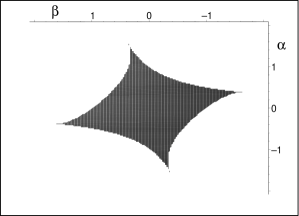
Figure 1: In the $\alpha-\beta$ plane the eigenvalues of matrix (17) only remain real inside the black domain.

Starting from $N=4$ it makes also sense to search for the multiply and, in particular, maximally degenerate EPs (MEPs), i.e., for the vertices of the spikes as seen in our two-dimensional Fig. 1. The required algorithm may be entirely universal. Indeed, as long as all of the roots $s_{n}$, $n=1,2,\ldots,N$ of our secular equation must degenerate to zero at MEPs, each coefficient in the secular polynomial must vanish (up to the leading one of course). One obtains a multiplet of polynomial equations, perfectly fitting the capabilities of the Gröbner-basis reduction and elimination techniques [18].

The $N=4$ example is already sufficiently instructive because its two MEP conditions derived from secular Eq. (18) form a nontrivial coupled pair of polynomial equations

$$\alpha^{2}+\beta^{2}=3\,,\ \ \ \ \ \ \ \ \alpha^{2}=(1+\alpha\beta)^{2}\,.$$ (19)

Under a proper account of symmetries the Gröbner-basis elimination provides the effective quartic polynomial equation

$$2-6\,\beta+2\,{\beta}^{2}+2\,{\beta}^{3}-{\beta}^{4}=0$$

possessing the two complex and two real MEP roots. Their numerical localization enables us, finally, to find the exact coordinates of the four spikes in Fig. 1, viz.,

$$\beta=\pm 1.691739510\,,\ \ \ \ \ \ \alpha=\mp 0.3715069717$$

$$\beta=\pm 0.4060952085\,,\ \ \ \ \ \ \alpha=\pm 1.683771565.$$

No genuine methodical news appear during the transition to the more realistic as well as more complicated secular equations at any larger $N>4$.

4.2 The new BIM and NNIM models of paragraphs 2.2 and 2.3, respectively

As long as the one- or few-parametric GPM Hamiltonian matrices of paragraph 2.2 may be perceived as mere special cases of the fully general multi-parametric NNIM $N$ by $N$ matrices of paragraph 2.3, both of these dynamical scenarios may be studied in parallel. Also the majority of observations of subsection 4.1 may be taken over without truly essential changes. Thus, for our first nontrivial $N=4$ illustrative example (8) the energy spectrum coincides with the roots of the following elementary secular equation

$${{\it E}}^{4}+\left({\alpha}^{2}-3+2\,{\beta}^{2}\right){{\it E}}^{2}+1-2\,{\beta}^{2}+{\beta}^{4}=0\,.$$

These energies will occur in pairs $E_{\pm,\pm}=\pm\sqrt{Z_{\pm}}$ where the symbol $Z_{\pm}$ denotes the two easily deduced roots of quadratic equation. As above, the latter two roots must be non-negative inside the closure of the physical parametric domain ${\cal D}$. Thus, mutatis mutandis one can repeat the construction steps as made in preceding subsection. At any dimension $N$ these steps involve again the comprehensive graphical analysis of the energy spectra as well as the explicit Gröbner-basis constructions of the MEP parameters.

Our enthusiasm over the efficiency of algorithms gets enhanced by the wealth of complexity of the topological structure of the spectral loci (cf. their graphical samples in Ref. [15]). Similar pleasant surprises also emerge in the MEP-construction perspective. Let us display one of the results in which the tedious Gröbner-basis constructive effort resulted in an amazing $N\to N+1$ extrapolation hypothesis. The essence of this new scenario is best illustrated by the following $N=10$ example

$$\left[\begin{array}[]{cccccccccc}2&-1-t&0&0&0&0&0&0&0&0\\ \vskip 6.0pt plus 2.0pt minus 2.0pt\cr-1+t&2&-1+t&0&0&0&0&0&0&0\\ \vskip 6.0pt plus 2.0pt minus 2.0pt\cr 0&-1-t&2&-1-t&0&0&0&0&0&0\\ \vskip 6.0pt plus 2.0pt minus 2.0pt\cr 0&0&-1+t&2&-1+t&0&0&0&0&0\\ \vskip 6.0pt plus 2.0pt minus 2.0pt\cr 0&0&0&-1-t&2&-1-t&0&0&0&0\\ \vskip 6.0pt plus 2.0pt minus 2.0pt\cr 0&0&0&0&-1+t&2&-1+t&0&0&0\\ \vskip 6.0pt plus 2.0pt minus 2.0pt\cr 0&0&0&0&0&-1-t&2&-1-t&0&0\\ \vskip 6.0pt plus 2.0pt minus 2.0pt\cr 0&0&0&0&0&0&-1+t&2&-1+t&0\\ \vskip 6.0pt plus 2.0pt minus 2.0pt\cr 0&0&0&0&0&0&0&-1-t&2&-1-t\\ \vskip 6.0pt plus 2.0pt minus 2.0pt\cr 0&0&0&0&0&0&0&0&-1+t&2\end{array}\right]\,$$ (20)

for which the $t-$dependence of the spectrum is shown in Fig. 2.

Figure 2: Real eigenvalues of Hamiltonian (20) exhibiting the two phase-transition MEP complexification singularities at $t=\pm 1$.

5 Remarks on the constructions of metrics

The explicit constructive assignment of a nontrivial metric $\Theta\neq I$ to a given Hamiltonian $H$ with real spectrum is not easy even at $N<\infty$ and even with the assistance of computers. In one of the most ambitious approaches to this problem (as accepted also in paper I) the general assignment of a metric $\Theta$ to the given Hamiltonian $H$ relies on the brute-force solution of the set of $N^{2}$ linear-algebraic equations (29) of Appendix A. The technical details of such an assignment remain nontrivial (cf. [19]).

There exist several successful strategies of the explicit evaluation of solutions $\Theta=\Theta(H)$. As mentioned, one of them consists in a linear-algebraic approach to Eq. (29) of Appendix A. It may prove to be the most efficient one, especially in sparse-matrix models [20]. An alternative recipe is offered by the spectral-type expansion formula

$$\Theta=\Theta(H,\vec{\kappa})=\sum_{j=0}^{N-1}\,|\Xi_{j}\rangle\,\kappa_{n}\,\langle\Xi_{j}|\,$$ (21)

where symbols $|\Xi_{j}\rangle$ denote the eigenkets of the conjugate operator $H^{\dagger}$ while the optional parameters $\kappa_{j}>0$ remain arbitrary [21].

For illustration let us now return, once more, to the discrete AOM quantum system. The model can only be declared completed after the Hamiltonian $H$ had been complemented by the selection of the Hilbert-space metric $\Theta$. In paper I we showed that the construction of such a metric is, with the assistance of sophisticated computer-mediated symbolic manipulations, feasible even if complicated. The brute-force strategy with $N^{2}$ linear equations has been recommended there. Due to the natural limitations of the display of formulae we merely replaced the printout of metrics by the more compact (and, for reconstruction, sufficient) presentation of the mere $N-$plets of eigenvectors $|\Xi_{j}\rangle$.

Once we now have to move to a sample application of the two alternative recipes to the three new models, let us pick up just the one of paragraph 2.3 for the sake of definiteness. In contrast to paper I where we were mainly interested in the physics of quantum catastrophes (for which the knowledge of the metric proved essential), we are now mainly interested in the same problem from the point of view of computer-assisted mathematics. While our present main interest remained concentrated on the genuinely non-linear problems of section 4, such a change of point of view also implies a definite weakening of our interest in the linear-algebraic problem of solution of Eq. (29) for the metric.

This being said we may now recall our particular $N=4$ illustrative example (8) and reveal that the construction of the metric leads to challenging problems. Let us explain the essence of one of them which refers to both of the above alternative approaches. The core of the message will lie in the construction which assigns the two different metrics to the same Hamiltonian in dependence of the choice of parameters from inside ${\cal D}$.

In the first step, in the spirit of Ref. [20] one can show that for any pair of “small” dynamical parameters $\alpha\in(-1,1)$ and $\beta\in(-1,1)$ one of the metrics for Hamiltonian (8) may be chosen diagonal (i.e., $\Theta_{ij}=0$ iff $i\neq j$). This choice is well defined and unique so that any other non-equivalent positive definite metric $\Theta(H)$ must necessarily acquire a non-diagonal matrix form.

Now one reveals a paradox by picking up a special version of quantum Hamiltonian (8) in which we choose a “small” $\alpha=\alpha_{0}=1/2$ and “large” $\beta=\beta_{0}=3\sqrt{2}/4\approx 1.060660172>1$. Then we easily verify that the whole spectrum of energies remains real and that it may even be written in closed form, $E_{\pm,\pm}=(\pm 1\pm\sqrt{3})/4$. Still, as long as $1.060660172>1$, the simplest possible diagonal-metric anssatz would not work anymore in this regime – it will simply fail to remain positive definite. Such a conclusion declares the use of the brute-force method useless in the whole domain of parameters ${\cal D}$. In some of its parts, a return to the robust spectral-like formula (21) emerges as unavoidable.

As long as the eigenvectors of $H^{\dagger}$ as needed in (21) are not mutually orthogonal, the alternative metrics need not be sparse matrices anymore. The resulting closed and entirely general four-parametric form (21) of metric $\Theta=\Theta(H,\vec{\kappa})$ cannot be printed on a single page as a consequence. Thus, one only has to display the explicit eigenvectors in place of the whole matrix of metric. For illustration we may pick up the sample values of $\alpha=\alpha_{0}=1/2$ and $\beta=\beta_{0}=3\sqrt{2}/4$ and show that the resulting eigenvectors still remain compact and easily displayed,

$$|\Xi_{++}\rangle=\left(\begin{array}[]{c}2+3\,\sqrt{2}-2\,\sqrt{3}-6\,\left(1/4+1/4\,\sqrt{3}\right)\sqrt{2}\\ 1\\ -1/3\,\sqrt{3}\\ 2-2/3\,\sqrt{3}-2\,\sqrt{2}+2\,\left(1/4+1/4\,\sqrt{3}\right)\sqrt{2}\end{array}\right)\,,$$ (22)

$$|\Xi_{+-}\rangle=\left(\begin{array}[]{c}2+3\,\sqrt{2}+2\,\sqrt{3}-6\,\left(1/4-1/4\,\sqrt{3}\right)\sqrt{2}\\ 1\\ 1/3\,\sqrt{3}\\ 2+2/3\,\sqrt{3}-2\,\sqrt{2}+2\,\left(1/4-1/4\,\sqrt{3}\right)\sqrt{2}\end{array}\right)\,,$$ (23)

$$|\Xi_{-+}\rangle=\left(\begin{array}[]{c}-2-3\,\sqrt{2}-2\,\sqrt{3}-6\,\left(-1/4+1/4\,\sqrt{3}\right)\sqrt{2}\\ 1\\ -1/3\,\sqrt{3}\\ 2+2/3\,\sqrt{3}-2\,\sqrt{2}-2\,\left(-1/4+1/4\,\sqrt{3}\right)\sqrt{2}\end{array}\right)\,,$$ (24)

$$|\Xi_{--}\rangle=\left(\begin{array}[]{c}-2-3\,\sqrt{2}+2\,\sqrt{3}-6\,\left(-1/4-1/4\,\sqrt{3}\right)\sqrt{2}\\ 1\\ 1/3\,\sqrt{3}\\ 2-2/3\,\sqrt{3}-2\,\sqrt{2}-2\,\left(-1/4-1/4\,\sqrt{3}\right)\sqrt{2}\end{array}\right)\,.$$ (25)

Their insertion in the general four-parametric formula (21) would be straightforward, confirming the efficiency of the computer-assisted manipulations in dealing with the problems of quantum catastrophes within the overall PTQM theoretical framework.

6 Conclusions

Via several families of solvable models we showed that besides the well known role of the numerical calculations and besides the standard use of graphics, the tools of computer-assisted algebra and symbolic manipulations might also prove particularly useful and productive in quantitative and theoretical analyses of many sufficiently elementary quantum systems and phenomena.

Our main attention has been paid to the study of behavior of a triplet of toy models near their horizons of observability $\partial{\cal D}^{(N)}$. In this light, the physics-oriented readers of this MS might ask questions about the practical phenomenological applicability of the models. Let us, therefore, fill the gap and let us touch this question in this section.

Firstly, let us mention that many years ago, the primary source of interest in quantum models possessing EP singularities emerged within the broad framework of perturbation calculations. Although the most influential Kato’s monograph [8] on perturbation series was not strictly aimed at physicists (typically, Barry Simon bitterly complained, as a student, that he had to study the Kato’s non-Hermitian examples), it left a lasting impact in the field (one of main reasons was that the EP positions in the complex plane of couplings determined, mathematically, the radii of convergence of the series).

Many years later, the majority of quantum physicists still considered the Kato’s introduction of his EP concept via $N=2$ real matrices rather formal. Nevertheless, these special definitions of the simplest possible square-root-type EP singularities found in fact numerous applications in a fairly broad variety of quantum as well as non-quantum physical contexts (cf., e.g., the webpage [22] of a recent dedicated international conference).

In comparison, not too much attention has still been paid to the EP singularities of the higher degeneracy. In many practical realizations of these degeneracies there emerges a fine-tuning problem because the mere random variation of phenomenological parameters offers just very small chances of a fusion of the simple EP singularities (forming, at $N>2$, the higher-order-EP or multiple EP alias MEP degeneracies).

The latter argument looks persuasive [23]. It seems to have kept the theoretical studies as well as experimental simulations of the MEP-related phenomena out of the mainstream in contemporary physics until very recently. Currently, the scepticism may be weakening. A particularly encouraging physics-oriented sample of the potentially important applications of the MEP-related ideas has been presented, for example, in preliminary report [24]. In this text one of us argued that the formalism of PTQM might be able to offer a long-needed innovative conceptual ground for the unification of the classical Big Bang evolution scenario with the standard principles of quantum theory in theoretical cosmology.

In paper I [9] the latter idea was prepared and developed beyond the simplest examples. In order to make any attempted application feasible one still had to restrict attention to the Hilbert spaces with finite dimensions. On conceptual level this already enabled one of us to establish, i.a., one of the first successful connections of quantum mechanics with the classical Thom’s theory of catastrophes (cf. [25]).

The key mathematical message of paper I was that the availability of the optional and, in principle, variable metric $\Theta^{(S)}$ which defines the inner product in the standard Hilbert space ${\cal H}^{(S)}$ opens the way towards an innovated, deeply quantum-theoretical concept of a quantum catastrophe. During such a catastrophe the very Hilbert space ${\cal H}^{(S)}$ ceases to exist. In the present continuation of the theory we complemented paper I by a number of further models and by the description of a few technical details including also illustrative explicit constructions.

In a slightly sceptical mood we should add that in contrast to the discrete anharmonic oscillator model as used in paper I, the present three new discrete-lattice models proved slightly less user friendly. The truly unique and exceptional close-form MEP roots of paper I had to be replaced, in places, by the mere numerical roots of the analogous effective polynomials (cf., e.g., the end of paragraph 4.1 for our present illustrative example).

In the broader physical area of a realistic phenomenology a lot of work still remains to be done as well. The main reason is that at the present stage of development the PTQM approach is still characterized by the technical difficulties given by the fact that $\Theta\neq I$. Anyhow, we believe that a systematic analysis of these difficulties is both necessary and feasible. In this sense, one of our main conclusions is that for the time being, the best chances of an imminent progress are still just in a continued study of the finite-dimensional Hilbert spaces and of the special families of models.

Appendix A: A brief account of the PTQM formalism

A.1. Introduction of sophisticated Hilbert spaces ${\cal H}^{(S)}$ with nontrivial physical inner products

In the Bender’s and Boettcher’s PTQM quantum theory one replaces Eq. (2) by a less usual but, presumably, “friendlier” Schrödinger equation

$${\rm i}\partial_{t}\,|\psi^{(F)}\rangle=H\,|\psi^{(F)}\rangle\,$$ (26)

where $|\psi^{(F)}\rangle\,\in\,{\cal H}^{(F)}\,$ and where the Hamiltonian is allowed non-Hermitian, $H\neq H^{\dagger}$. It is only required that $H$ possesses a real and non-degenerate bound-state-type spectrum. The basic mathematical idea of the PTQM theory may be then formulated as a natural rejection of the “first” Hilbert space ${\cal H}^{(F)}$ as “false” and unphysical, i.e., as yielding a manifestly non-unitary evolution of the system in question via Eq. (26). Once we want to interpret Eq. (26) as fully compatible with any textbook on quantum mechanics, we simply must move to an amended, “second” Hilbert space ${\cal H}^{(S)}$ [7].

The first condition of consistency of such a procedure is that the two Hilbert spaces ${\cal H}^{(F)}$ and ${\cal H}^{(S)}$ only differ from each other by the definition of the respective inner products. With no difference between the ket-vectors themselves, $|\psi^{(S)}\rangle\ \equiv\ |\psi^{(F)}\rangle\$, the change only involves the linear functionals (i.e., the so called bra-vectors). Thus, one simply replaces the common (a.k.a. “Dirac’s”) anti-linear Hermitian-conjugation operation

$${\cal T}^{(F)}:|\psi^{(F)}\rangle\ \to\langle\psi^{(F)}|$$ (27)

valid in ${\cal H}^{(F)}$ by its alternative

$${\cal T}^{(S)}:|\psi^{(S)}\rangle\ \to\langle\!\langle\psi^{(S)}|\ \equiv\ \langle\psi^{(F)}|\,\Theta\,$$ (28)

valid in the “standard” physical Hilbert-space ${\cal H}^{(S)}$ (cf. also [4] for more details). The purpose of the introduction of the latter general formula which contains an optional Hilbert-space metric operator $\Theta=\Theta^{\dagger}>0$ is that an appropriate choice of the metric $\Theta$ must make our Hamiltonian $H$ self-adjoint in ${\cal H}^{(S)}$. Mathematically speaking [20] one must merely guarantee the validity of the Dieudonné’s compatibility condition

$$H^{\dagger}\,\Theta=\Theta\,H\,.$$ (29)

The key problem of the assignment of a suitable Hermitizing metric $\Theta$ to a given non-Hermitian Hamiltonian $H$ is that the Dieudonné’s constraint (29) still leaves the metric $\Theta=\Theta(H)$ (and, hence, the physical inner product and the physical Hilbert space ${\cal H}^{(S)}$) non-unique. Fortunately, according to the older review [7] the resolution of the problem is imminent. One merely specifies a $K-$plet of additional observables ${\cal C}_{j}$, $j=1,2,\ldots,K$ with such a count $K$ that the metric (which makes them all self-adjoint) becomes unique.

A.2. ${\cal PT}-$symmetric quantum systems

A hidden reason of the recent success and appeal of the PTQM formalism in applications [2] may be traced back to its trademark use of an additional, heuristically enormously productive assumption

$$H^{\dagger}{\cal P}={\cal P}\,H\,.$$ (30)

This means that our Hamiltonian operator $H$ is required self-adjoint in another, associated Krein space ${\cal K}$ which is defined as endowed with an indefinite metric (i.e., pseudo-metric) ${\cal P}$ [3, 26]. Relation (30) re-written in its formally equivalent and, among physicists, perceivably more popular representation $H{\cal PT}={\cal PT}\,H\,$ explains the words “${\cal PT}-$symmetry of $H$”.

The uniqueness of the physical interpretation of ${\cal PT}-$symmetric quantum models is often based on the $K=1$ postulate of existence of a single “missing observable” ${\cal C}_{1}$, exhibiting all of the characteristics of a charge (cf. [2] for a virtually exhaustive account of this version of the theory). In our present paper a less widespread strategy of making the metric unique is taken from paper I.

Appendix B. BIM - GPM correspondence at large $N$

In Eq. (7) the inner subvector $Q|\psi\rangle$ with $(N-4)$ components $\{\psi_{3},\ldots,\psi_{N-2}\}$ may be interpreted as an exact solution of an incomplete set of the standard discrete free-motion conditions

$$-\triangle\psi_{k}=E\,\psi_{k}\,,\ \ \ k=3,4,\ldots,N-2\,.$$ (31)

Whenever this middle-partition vector $Q|\psi\rangle$ is given in advance, then, on the contrary, the third line of Eq. (7) may be re-read as the definition of component $\psi_{2}$ while the $(N-2)$nd line defines $\psi_{N-1}$. At this moment we are left just with the remaining first two rows of our equation,

$$2\psi_{1}-(1+\lambda)\psi_{2}\ \equiv\ \psi_{1}+\delta\psi_{3/2}-\lambda\,\psi_{2}=E\,\psi_{1}\,,$$

$$(-1+\lambda)\psi_{1}+(2-E)\,\psi_{2}-\psi_{3}\ \equiv\ (-\triangle-E)\psi_{2}+\lambda\psi_{1}=0\,$$

plus, mutatis mutandis, with the last two rows. In terms of the not yet specified parameter $\delta\psi_{3/2}$ the first row enables us to define the last ket-vector component $\psi_{1}$. Once we eliminate $\psi_{1}$ from the second row, we obtain

$$(1-E)(-\triangle-E)\psi_{2}=\lambda^{2}\psi_{2}-\lambda\,\delta\psi_{3/2}\,.$$ (32)

At the large dimensions $N\gg 1$, the latter relation may now be quite naturally re-read as an extension of Eq. (31) to $k=2$, based on a self-consistency condition

$$\lambda\psi_{2}-\delta\psi_{3/2}=0\,.$$ (33)

Now one may recall the most natural approximate, large$-N$ identification of the matrix indices $j=1,2,\ldots,N$ with the suitable equidistant grid points of a real interval. In the corresponding map $j\to x_{j}=x_{0}+jh$, the constant $h>0$ is assumed small, $h\sim 1/N$.

In the limit of large $N$, the ket-vector elements $\psi_{j}$ may be then re-read as the values of a wave function $\psi(x)$ at the respective coordinate $x=x_{j}$. Similarly, relation (33) acquires the simplified meaning of the so called Robin’s boundary condition at $x=x_{0}$,

$$\lambda\psi(x_{0})-\partial_{x}\psi(x_{0})=0\,.$$ (34)

A close connection emerges with the local-interaction model of Ref. [13]. It is worth adding that the latter, manifestly non-Hermitian model found an interesting immediate physical interpretation via an R-matrix description of one-dimensional quantum scattering [27, 28]. These observations may be also read as another encouragement of the study of the multiparametric NNIM generalizations of the one-parametric BIM model (7).

References

- [1] Dorey, P., Dunning, C., Tateo, R.: Spectral equivalences, Bethe Ansatz equations, and reality properties in -symmetric quantum mechanics. J. Phys. A: Math. Gen. 34, 5679–5704 (2001)
- [2] Bender, C. M.: Making sense of non-hermitian Hamiltonians. Rep. Prog. Phys. 70, 947–1018 (2007); Dorey, P., Dunning, C., Tateo, R.: The ODE/IM correspondence. J. Phys. A: Math. Theor. 40, R205–R283 (2007)
- [3] Mostafazadeh, A.: Pseudo-Hermitian Representation of Quantum Mechanics. Int. J. Geom. Meth. Mod. Phys. 7, 1191–1306 (2010)
- [4] Znojil, M.: Three-Hilbert-space formulation of Quantum Mechanics. Symmetry, Integrability and Geometry: Methods and Applications 5, 001, 19 pages (2009)
- [5] Bender, C.M., Boettcher, S.: Real Spectra in Non-Hermitian Hamiltonians Having PT Symmetry. Phys. Rev. Lett. 80, 5243 5246 (1998)
- [6] Siegl, P., D. Krejčiřík, D.: On the metric operator for the imaginary cubic oscillator. Phys. Rev. D 86, 121702(R) (2012)
- [7] Scholtz, F.G., Geyer, H.B., Hahne, F.J.H.: Quasi-Hermitian Operators in Quantum Mechanics and the Variational Principle. Ann. Phys. (NY) 213, 74–101 (1992)
- [8] Kato,T.: Perturbation theory for linear operators. Spinger, Berlin (1966)
- [9] Znojil, M.: Quantum catastrophes: a case study. J. Phys. A: Math. Theor. 45, 444036 (2012)
- [10] Znojil, M.: N-site-lattice analogues of . Ann. Phys. (NY) 327, 893–913 (2012)
- [11] Jones, H.F.: Interface between Hermitian and non-Hermitian Hamiltonians in a model calculation. Phys. Rev. D 78, 065032 (2008)
- [12] Znojil, M.: Scattering theory with localized non-Hermiticities. Phys. Rev. D 78, 025026 (2008)
- [13] Krejčiřík, D., Bíla, H., Znojil, M.: Closed formula for the metric in the Hilbert space of a -symmetric model. J. Phys. A: Math. Gen. 39, 10143–10153 (2006)
- [14] Znojil, M.: Complete set of inner products for a discrete -symmetric square-well Hamiltonian. J. Math. Phys. 50, 122105 (2009)
- [15] Znojil, M., Wu, J.: Int. J. Theor. Phys. 52, 2152–2162 (2013).
- [16] Znojil, M.: Solvable model of quantum phase transitions and the symbolic-manipulation-based study of its multiply degenerate exceptional points and of their unfolding. Ann. Phys. (NY) 336, 98–111 (2013).
- [17] Znojil, M.: Maximal couplings in -symmetric chain-models with the real spectrum of energies. J. Phys. A: Math. Theor. 40, 4863–4875 (2007)
- [18] Char, B. W. et al: Maple V Language Reference Manual. Springer, New York (1993)
- [19] Znojil, M.: Symbolic-manipulation constructions of Hilbert-space metrics in quantum mechanics. Lecture Notes in Computer Science 6885, 348–357 (2011)
- [20] Znojil, M.: Quantum inner-product metrics via recurrent solution of Dieudonne equation. J. Phys. A: Math. Theor. 45, 085302 (2012)
- [21] Znojil, M.: On the role of the normalization factors and of the pseudo-metric P in crypto-Hermitian quantum models. SYMMETRY, INTEGRABILITY and GEOMETRY: METHODS and APPLICATIONS SIGMA 4, 001 (2008)
- [22] http://www.nithep.ac.za/2g6.htm
- [23] Heiss, W.D.: The physics of exceptional points. J. Phys. A: Math. Theor. 45, 444016 (2012)
- [24] M. Znojil, M.: Quantum Big Bang without fine-tuning in a toy-model. J Phys: Conf. Ser. 343, 012136 (2012)
- [25] Thom, R.: Structural stability and morphogenesis. An outline of a general theory of models. Benjamin, Reading (1975); Arnold, V.I.: Catastrophe Theory. Springer-Verlag, Berlin (1992)
- [26] Langer, H., Tretter, C.: A Krein space approach to PT symmetry. Czechosl. J. Phys. 70, 1113 1120 (2004); Krejčiřík, D., Siegl, P., Železný, J.: On the similarity of Sturm-Liouville operators with non-Hermitian boundary conditions to self-adjoint and normal operators. Complex Anal. Oper. Theory, to appear (arXiv:1108.4946).
- [27] Hernandez-Coronado, H., Krejčiřík, D., Siegl, P.: Perfect transmission scattering as a -symmetric spectral problem. Phys. Lett. A 375, 2149–2152 (2011)
- [28] Ambichl, P., Makris, K. G., Ge, L., Chong, Y.-D., Stone, A. D., Rotter, S.: Breaking of PT Symmetry in Bounded and Unbounded Scattering Systems. Phys. Rev. X 3, 041030 (2013) [9 pages].