Relativistic electrons and magnetic field of the M87 jet on $\sim$ten Schwarzschild radii scale

Abstract

We explore energy densities of magnetic field and relativistic electrons in the M87 jet. Since the radio core at the jet base is identical to the optically thick surface against synchrotron self absorption (SSA), the observing frequency is identical to the SSA turnover frequency. As a first step, we assume the radio core as a simple uniform sphere geometry. Using the observed angular size of the radio core measured by the Very Long Baseline Array at 43 GHz, we estimate the energy densities of magnetic field ($U_{B}$) and relativistic electrons ($U_{e}$) based on the standard SSA formula. Imposing the condition that the Poynting power and relativistic electron one should be smaller than the total power of the jet, we find that (i) the allowed range of the magnetic field strength ($B_{\rm tot}$) is $1~{}{\rm G}\leq B_{\rm tot}\leq 15~{}{\rm G}$, and that (ii) $1\times 10^{-5}\leq U_{e}/U_{B}\leq 6\times 10^{2}$ holds. The uncertainty of $U_{e}/U_{B}$ comes from the strong dependence on the angular size of the radio core and the minimum Lorentz factor of non-thermal electrons ($\gamma_{e,\rm min}$) in the core. It is still open that the resultant energetics is consistent with either the magnetohydrodynamic jet or with kinetic power dominated jet even on $\sim 10$ Schwarzschild radii scale.

1. Introduction

Formation mechanism of relativistic jets in active galactic nuclei (AGNs) remains as a longstanding unresolved problem in astrophysics. Although the importance of magnetic field energy density ($U_{\rm B}$) and relativistic electron one ($U_{e}$) for resolving the formation mechanism has been emphasized (e.g., Blandford and Rees 1978), it is not observationally clear whether either $U_{\rm B}$ or $U_{e}$ is dominant at the jet base. Relativistic magnetohydrodynamics models for relativistic jets generally assume highly magnetized plasma at the jet base (e.g., Koide et al. 2002; Vlahakis and Konigl 2003; McKinney and Gammie 2004; Krolik et al. 2005; McKinney 2006; Komissarov et al. 2007; Tchekhovskoy et al. 2011; Toma and Takahara 2013; Nakamura and Asada 2013), while an alternative model assumes a pair plasma dominated “fireball”-like state at the jet base (e.g., Iwamoto and Takahara 2002; Asano and Takahara 2009 and reference therein). Although deviation from equi-partition (i.e., $U_{e}/U_{B}\approx 1$) is essential for investigation of relativistic jet formation, none has succeeded in obtaining a robust estimation of $U_{e}/U_{B}$ at the jet base.

M87, a nearby giant radio galaxy located at a distance of $D_{\rm L}=16.7~{}{\rm Mpc}$ (Jordan et al. 2005), hosts one of the most massive super massive black hole $M_{\bullet}=(3-6)\times 10^{9}~{}M_{\odot}$ (e.g., Macchetto et al. 1997; Gebhardt and Thomas 2009; Walsh et al. 2013). Because of the largeness of the angular size of its central black hole, M87 is well known as the best source for imaging the deepest part of the jet base (e.g., Junor et al. 1999). Furthermore, M87 has been well studied at wavelengths from radio to Very High Energy (VHE) $\gamma$-ray (Abramowski et al. 2012; Hada et al. 2012 and reference therein) and causality arguments based on VHE $\gamma$-ray outburst in February 2008 indicate that the VHE emission region is less than $\sim 5\delta~{}{\rm R_{s}}$ where $\delta$ is the relativistic Doppler factor (Acciari et al. 2009). The Very-Long-Baseline-Array (VLBA) beam resolution at 43 GHz typically attains about $0.21\times 0.43~{}{\rm mas}$ which is equivalent to $5.3\times 10^{16}\times 1.1\times 10^{17}~{}{\rm cm}$. When $M_{\bullet}=6\times 10^{9}~{}M_{\odot}$ holds (Gebhardt et al. 2009), then VLBA beam resolution approximately corresponds to $30\times 60~{}{\rm R_{s}}$. Recent progresses of Very-Long-Baseline-Interferometry (VLBI) observations have revealed the inner jet structure, i.e., frequency and core-size relation, and distance and core-size relation down to close to $\sim 10$ Schwarzschild radii ($R_{\rm s}$) scale (Hada et al. 2011, hereafter H11). Thus, the jet base of M87 is the best laboratory for investigations of $U_{e}/U_{B}$ in the real vicinity of the central engine.

Two significant forward steps are recently obtained in M87 observations which motivate the present work. First, Hada et al. (2011) succeeded in directly measuring core-shift phenomenon at the jet base of M87 at 2, 5, 8, 15, 24 and 43 GHz. The radio core position at each frequency has been obtained by the astrometric observation (H11). Since the radio core surface corresponds to the optically-thick surface at each frequency, the synchrotron-self-absorption (SSA) turnover frequency $\nu_{\rm ssa}$ is identical to the observing frequency itself. Second, we recently measure core sizes in Hada et al. (2013a) (hereafter H13). Hereafter we focus on the radio core at 43 GHz. In H13, we select VLBA data observed after 2009 with sufficiently good qualities (all 10 stations participated and good uv-coverages). To measure the width of the core, a single, full-width-half-maximum (FWHM) Gaussian is fitted for the observed radio core at 43 GHz in the perpendicular direction to the jet axis and we derive the width of the core ($\theta_{\rm FWHM}$). We stress that the core width is free from the uncertainty of viewing angle. Therefore, using $\theta_{\rm FWHM}$ at 43 GHz, we can estimate values of $U_{e}/U_{B}$ in the 43 GHz core of M87 for the first time.

In section 2, we derive an explicit form of $U_{e}/U_{B}$ by using the standard formulae of synchrotron absorption processes. As a first step, we simplify a geometry of the radio core as a single uniform sphere although the real geometry is probably more complicated. In section 3, we estimate $U_{e}/U_{\rm B}$ in the M87 jet base by using the VLBA data at 43 GHz obtained in H13. In section 4, we summarize the result and discuss relevant implications. In this work, we define the radio spectral index $\alpha$ as $S_{\nu}\propto\nu^{-\alpha}$ and we assume $M_{\bullet}=6\times 10^{9}~{}M_{\odot}$.

2. Model

Here, we derive explicit expressions of the strength of total magnetic field $B_{\rm tot}$ and $U_{e}/U_{B}$. Several papers have extensively discussed the determination of magnetic field strength $B_{\rm tot}$. Fundamental formulae of SSA processes are shown in the following references and we follow them (Ginzburg and Syrovatskii 1965, hereafter GS65; Blumenthal and Gould 1970, hereafter BG70; Pacholczyk 1970, Rybicki and Lightman 1979, hereafter RL79). Here, we will show a simple derivation of the explicit expressions of $B_{\rm tot}$ and $U_{e}/U_{B}$ with sufficient accuracy.

2.1. Method

For clarity, we briefly summarize the method for determining $B_{\rm tot}$ and $U_{e}/U_{B}$ in advance. The theoretical unknowns related to the magnetic field and relativistic electrons in the observed radio core with its angular diameter $\theta_{\rm obs}$ are following four; $B_{\rm tot}$, $K_{e}$ (the normalization factor of non-thermal electron number density), $\gamma_{e,\rm min}$ (the minimum Lorentz factor of non-thermal electrons) , and $p$ (the spectral index of non-thermal electrons). Among them, $\gamma_{e,\rm min}$, and $p$ are directly constrained by radio observations at mm/sub-mm wavebands. The remaining $B_{\rm tot}$ and $K_{e}$ can be solved by using the two general relations which hold at $\nu=\nu_{\rm ssa}$ shown in Eqs. (3) and (4). The solved $B_{\rm tot}$ and $K_{e}$ are written as functions of $\theta_{\rm obs}$, $\gamma_{e,\rm min}$, $\nu_{\rm ssa}$, and the observed flux at $\nu=\nu_{\rm ssa}$.

Lastly, we further impose total jet power constraint not to overproduce Poynting- or kinetic-power shown in Eq. (3.3). This constraint can partially exclude larger value of $\theta_{\rm obs}$. Then, we can determine $B_{\rm tot}$ and $U_{e}/U_{\rm B}$ of M87 consistently.

2.2. Assumptions

Following assumptions are adopted in this work:

• We assume uniform and isotropic distribution of relativistic electrons and magnetic fields in the emission region. For M87, polarized flux does not seem very large. Therefore, we assume isotropic tangled magnetic field in this work. Hereafter, we denote $B$ as the magnetic field strength perpendicular to the direction of electron motion. Then, the total field strength is

  $$B_{\rm tot}=\sqrt{3}B.$$ (1)

  Hereafter, we define $U_{B}\equiv B_{\rm tot}^{2}/8\pi$.

• We assume the emission region is spherical with its radius $R$ measured in the comoving frame. The radius is defined as

  $$2R=\theta_{\rm obs}D_{A},$$ (2)

  where $D_{A}=D_{L}/(1+z)^{2}$ is the angular diameter distance to a source (e.g., Weinberg 1972). Because M87 is the very low redshift source, we only use $D_{A}$ throughout this paper. There might be a slight difference between $\theta_{\rm FWHM}$ and $\theta_{\rm obs}$. VLBI measured $\theta_{\rm FWHM}$ is conventionally treated as $\theta_{\rm obs}=\theta_{\rm FWHM}$, while Marscher (1983) pointed out a deviation expressed as $\theta_{\rm obs}\approx 1.8\theta_{\rm FWHM}$ which is caused by a forcible fitting of Gaussians to a non-Gaussian component. In this work, we introduce a factor $A$ defined as $\theta_{\rm obs}\equiv A\theta_{\rm FWHM}$ and $1\leq A\leq 1.8$ is assumed.

We stress that the uniform and isotropic sphere model is a first step simplification and the realistic jet base probably contains more complicated geometry and nonuniform distributions in magnetic field and electron density. We will investigate such complicated cases in the future.

2.3. Synchrotron emissions and absorptions

In order to obtain explicit expression of $B$ and $K_{e}$ in terms of $\theta_{\rm obs}$, $\nu_{\rm ssa,obs}$, and $S_{\nu_{\rm ssa},\rm obs}$, here we briefly review synchrotron emissions and absorptions. At the radio core, $\tau_{\nu_{\rm ssa}}$ becomes an order of unity at $\nu=\nu_{\rm ssa}$;

$$\tau_{\nu_{\rm ssa}}=2\alpha_{\nu_{\rm ssa}}R,$$ (3)

where $\tau_{\nu_{\rm ssa}}$ and $\alpha_{\nu_{\rm ssa}}$ are the optical depth for SSA and the absorption coefficient for SSA, respectively. We impose that optically thin emission formula is still applicable at $\nu_{\rm ssa}$:

$$\frac{4\pi}{3}R^{3}\epsilon_{\nu_{\rm ssa}} = 4\pi R^{2}S_{\nu_{\rm ssa}},$$ (4)

where $\epsilon_{\nu_{\rm ssa}}$ and $S_{\nu_{\rm ssa}}$ are he emissivity and flux per unit frequency, respectively. Combining Eq. 4 and the approximation of $\tau_{\nu_{\rm ssa}}=1$, we can solve $B$ and $K_{e}$. This derivation is much simpler than previous studies of Marscher (1983) and Hirotani (2005) (hereafter H05). We will compare the derived $B_{\rm tot}$ in this work, Marscher (1983) and H05, and they will coincide with each other within a small difference in the range of $2.5\leq p\leq 3.5$.

Next, let us break down relevant physical quantities. The term $K_{e}$, the normalization factor of electron number density distribution $n_{e}(\gamma)$, is defined as (e.g., Eq.3.26 in GS65)

$$n_{e}(E_{e})dE_{e} = K_{e}E_{e}^{-p}dE_{e}\quad(E_{e,\rm min}\leq E_{e}\leq E_{e,\rm max}),$$

$$= \frac{K_{e}}{(m_{e}c^{2})^{p-1}}\gamma_{e}^{-p}d\gamma_{e}\quad(\gamma_{e,\rm min}\leq\gamma_{e}\leq\gamma_{e,\rm max}),$$

where $E_{e}=\gamma_{e}m_{e}c^{2}$ $p=2\alpha+1$, $E_{e,{\rm min}}=\gamma_{e,{\rm min}}m_{e}c^{2}$, and $E_{e,{\rm max}}=\gamma_{e,{\rm max}}m_{e}c^{2}$ are the electron energy, the spectral index, minimum energy, and maximum energy of relativistic (non-thermal) electrons, respectively. Let us further review optically thin synchrotron emissions. The maximum in the spectrum of synchrotron radiation from an electron occurs at the frequency: (Eq. 2.23 in GS65)

$$\nu_{\rm syn}=1.2\times 10^{6}B\gamma_{e}^{2}.$$ (6)

Synchrotron self-absorption coefficient measured in the comoving frame is given by (Eqs. 4.18 and 4.19 in GS65; Eq. 6.53 in RL79)

$$\alpha_{\nu} = \frac{\sqrt{3}e^{3}}{8\pi m_{e}}\left(\frac{3e}{2\pi m_{e}^{3}c^{5}}\right)^{p/2}c_{1}(p)$$ (7)

$$\times K_{e}B^{(p+2)/2}\nu^{-(p+4)/2},$$

where the numerical coefficient $c_{1}(p)$ is expressed by using the gamma-functions as follows; $c_{1}(p)=\Gamma[(3p+2)/12]\Gamma[(3p+22)/12]$. For convenience, we define $\alpha_{\nu}=X_{1}c_{1}(p)B^{(p+2)/2}K_{e}\nu^{-(p+4)/2}$.

Optically thin synchrotron emissivity per unit frequency $\epsilon_{\nu}$ from uniform emitting region is given by (Eqs. 4.59 and 4.60 in BG70; see also Eqs. 3.28, 3.31 and 3.32 in GS65)

$$\epsilon_{\nu} = 4\pi\frac{\sqrt{3}e^{3}}{8\sqrt{\pi}m_{e}c^{2}}\left(\frac{3e}{2\pi m_{e}^{3}c^{5}}\right)^{(p-1)/2}c_{2}(p)$$ (8)

$$\times K_{e}B^{(p+1)/2}\nu^{-(p-1)/2},$$

where the numerical coefficient is $c_{2}(p)=\Gamma[(3p+19)/12]\Gamma[(3p-1)/12)]\Gamma[(p+5)/4)]/\Gamma[(p+7)/4)]/(p+1)$. For convenience, we define $\epsilon_{\nu}\equiv 4\pi X_{2}c_{2}(p)B^{(p+1)/2}K_{e}\nu^{-(p-1)/2}$.

2.4. Relations between quantities measured in source and observer frames

Let us summarize the Lorentz transformations and cosmological effect using the Doppler factor ($\delta\equiv 1/(\Gamma(1-\cos\theta_{\rm LOS})$) where $\theta_{\rm LOS}$ is the angle between the jet and our line-of-sight) and the redshift ($z$). Hereafter, we put subscript (obs) for quantities measured at observer frame.

$$\nu_{\rm obs}=\nu\frac{\delta}{1+z}.$$ (9)

The observed flux from an optically thin source at a large distance is given by (Eq. 1.13 in RL79; Eqs. (7) in H05; see also Eq. C4 in Begelman et al. 1984):

$$S_{\nu_{\rm obs},\rm obs} = \left(\frac{\delta}{1+z}\right)^{3}S_{\nu}\left(\frac{\theta_{\rm obs}}{2}\right)^{2}.$$ (10)

2.5. Obtained $B$ and $K_{e}$

Combining the above shown relations, we finally obtain

$$B = b(p)\left(\frac{\nu_{\rm ssa,obs}}{1~{}{\rm GHz}}\right)^{5}\left(\frac{\theta_{\rm obs}}{1~{}{\rm mas}}\right)^{4}\left(\frac{S_{\nu_{\rm ssa},\rm obs}}{1~{}{\rm Jy}}\right)^{-2}$$ (11)

$$\times \left(\frac{\delta}{1+z}\right),$$

where the numerical value of $b(p)=[(2\times 3)/(4\pi)]^{2}(c_{2}(p)X_{2}/c_{1}(p)X_{1})^{2}$ are shown in Table 1. In the Table, we also note the values the obtained $b(p)$ with the ones in Marscher (1983) and H05. From this, we see that the derived $B_{\rm tot}$ in this work coincide with each other within the small difference.

Inserting Eq. (11) into Eq. (3) or Eq. (4), we then obtain $K_{e}$ as

$$K_{e} = k(p)\left(\frac{D_{\rm A}}{1~{}{\rm Gpc}}\right)^{-1}\left(\frac{\nu_{\rm ssa,obs}}{1~{}{\rm GHz}}\right)^{-2p-3}\left(\frac{\theta_{\rm obs}}{1~{}{\rm mas}}\right)^{-2p-5}$$ (12)

$$\times \left(\frac{S_{\nu_{\rm ssa},\rm obs}}{1~{}{\rm Jy}}\right)^{p+2}\left(\frac{\delta}{1+z}\right)^{-p-3},$$

where $k(p)=b(p)^{(-p-2)/2}X_{1}^{-1}c_{1}(p)^{-1}(D_{\rm A}/1~{}{\rm Gpc})^{-1}\nu_{\rm ssa,obs}^{(p+4)/2}$. The cgs units of $K_{e}$ and $k(p)$ depend on $p$: erg^p-1cm^-3. The numerical values of $k(p)$ are summarized in Table 1 and they are similar to the ones in Marscher (1983) which are $k(2.5)=1.2\times 10^{-2}$ and $k(3.0)=0.59\times 10^{-3}$. Using the obtained $K_{e}$, we can evaluate $U_{e}$ as

$$U_{e} = \int^{E_{e,\rm max}}_{E_{e,\rm min}}E_{e}n_{e}(E_{e})dE_{e}$$ (13)

$$= \frac{K_{e}E_{e,\rm min}^{-p+2}}{p-2}\quad({\rm for}\quad p>2).$$

Then, we can obtain the ratio $U_{e}/U_{B}$ explicitly as

$$\frac{U_{e}}{U_{B}} = \frac{8\pi}{3b^{2}(p)}\frac{k(p)E_{e,\rm min}^{-p+2}}{(p-2)}\left(\frac{D_{\rm A}}{1~{}{\rm Gpc}}\right)^{-1}\left(\frac{\nu_{\rm ssa,obs}}{1~{}{\rm GHz}}\right)^{-2p-13}$$ (14)

$$\times \left(\frac{\theta_{\rm obs}}{1~{}{\rm mas}}\right)^{-2p-13}\left(\frac{S_{\nu_{\rm ssa},\rm obs}}{1~{}{\rm Jy}}\right)^{p+6}\left(\frac{\delta}{1+z}\right)^{-p-5}$$

$$({\rm for}\quad p>2).$$

From this, we find that $\nu_{\rm ssa,obs}$ and $\theta_{\rm obs}$ have the same dependence on $p$. Using this relation, we can estimate $U_{e}/U_{B}$ without minimum energy (equipartition $B$ field) assumption. It is clear that the measurement of $\theta_{\rm obs}$ is crucial for determining $U_{e}/U_{B}$. We argue details on it in the next subsection. It is also evident that a careful treatment of $\gamma_{e,\rm min}$ is crucial for determining $U_{e}/U_{B}$ (Kino et al. 2002; Kino and Takahara 2004).

3. Application to M87

Based on recent VLBA observations of M87 at 43 GHz, we derive $U_{e}/U_{\rm B}$ at the base of M87 jet. Here, we set typical index of electrons as $p=3.0$ (Doi et al. 2013).

3.1. Electrons emitting 43 GHz radio waves

First, let us constrain on $\gamma_{e,\rm min}$. At least, $\gamma_{e,\rm min}$ should be smaller than the Lorentz factor of electrons radiating synchrotron emission at 43 GHz. Therefore, minimum Lorentz factor of electrons is constrained as

$$\gamma_{e,\rm min} \leq 2.0\times 10^{2}\left(\frac{\nu_{\rm ssa,obs}}{43~{}{\rm GHz}}\right)^{-2}\left(\frac{\theta_{\rm obs}}{0.11~{}{\rm mas}}\right)^{-2}$$ (15)

$$\times \left(\frac{S_{\nu_{\rm ssa},\rm obs}}{0.7~{}{\rm Jy}}\right)^{1}\left(\frac{\delta}{1+z}\right)^{-1}.$$

where we use Eqs. (6) and (9).

3.2. Normalized physical quantities

For convenience, we rewrite above quantities to normalized quantitates associated with the observed 43 GHz core. $B$ field inside the 43 GHz core is estimated as

$$B_{\rm tot} = 1.5~{}{\rm G}~{}\left(\frac{\nu_{\rm ssa,obs}}{43~{}{\rm GHz}}\right)^{5}\left(\frac{\theta_{\rm obs}}{0.11~{}{\rm mas}}\right)^{4}\left(\frac{S_{\nu_{\rm ssa},\rm obs}}{0.7~{}{\rm Jy}}\right)^{-2}$$ (16)

$$\times \left(\frac{\delta}{1+z}\right).$$

Here we use $0.11~{}{\rm mas}$ as a normalization of $\theta_{\rm FWHM}$. As mentioned in the Introduction, $\nu_{\rm ssa,obs}=43~{}{\rm GHz}$ holds at the 43 GHz core surface, because of the clear detection of the core shift phenomena in H11. As for $K_{e}$, we obtain

$$K_{e} = 1.6\times 10^{-6}~{}{\rm erg^{2}~{}cm^{-3}}~{}\left(\frac{\nu_{\rm ssa,obs}}{43~{}{\rm GHz}}\right)^{-9}\left(\frac{\theta_{\rm obs}}{0.11~{}{\rm mas}}\right)^{-11}$$ (17)

$$\times \left(\frac{S_{\nu_{\rm ssa},\rm obs}}{0.7~{}{\rm Jy}}\right)^{5}\left(\frac{\delta}{1+z}\right)^{-6}\left(\frac{D_{\rm A}}{16.7~{}{\rm Mpc}}\right)^{-1}.$$

Then, we finally obtain $U_{e}/U_{B}$ as

$$\frac{U_{e}}{U_{B}} = 2.2~{}\left(\frac{\nu_{\rm ssa,obs}}{43~{}{\rm GHz}}\right)^{-19}\left(\frac{\theta_{\rm obs}}{0.11~{}{\rm mas}}\right)^{-19}$$ (18)

$$\times \left(\frac{S_{\nu_{\rm ssa},\rm obs}}{0.7~{}{\rm Jy}}\right)^{9}\left(\frac{\delta}{1+z}\right)^{-8}\left(\frac{\gamma_{e,\rm min}}{10}\right)^{-1}$$

$$\times \left(\frac{D_{\rm A}}{16.7~{}{\rm Mpc}}\right)^{-1}.$$

This typical $U_{e}/U_{B}$ apparently shows the order of unity but it has strong dependences on $\theta_{\rm obs}$ and $\nu_{\rm ssa}$. Regarding $\nu_{\rm ssa,obs}$, an uncertainty only comes from the bandwidth. In our VLBA observation, the bandwidth is $128~{}{\rm MHz}$ with its central frequency 43.212 GHz. Therefore, it causes only a very small uncertainty $\sim(43.276/43.148)^{19}=1.06$. The accuracy of flux calibration of VLBA can be conservatively estimated as $10~{}\%$. An intrinsic flux of the radio core at 43 GHz also fluctuates with an order of $10~{}\%$ during a quiescent phase (e.g., Acciari et al. 2009; Hada et al. 2012). Therefore, the flux term also causes an uncertainty of $\sim 1.21^{9}=5.6$. The angular size $\theta_{\rm obs}$ and $\gamma_{e,\rm min}$ have much larger ambiguities than those evaluated above and we derive $U_{e}/U_{\rm B}$ by taking into account of these ambiguities in the next sub-section. At the same time, we again emphasize that $\theta_{\rm obs}$ obtained in H13 can be bearable for the estimate of $U_{e}/U_{\rm B}$ in spite of such strong dependence on $\theta_{\rm obs}$.

3.3. On $\theta_{\rm obs}$, $p$, and $L_{\rm jet}$

The most important quantity for the estimate of $U_{e}/U_{\rm B}$ is $\theta_{\rm obs}$. Based on VLBA observation data with sufficiently good qualities, here we set

$$0.11~{}{\rm mas}\leq\theta_{\rm obs}\leq 0.20~{}{\rm mas},$$ (19)

where we use the average value $\theta_{\rm FWHM}=0.11~{}{\rm mas}$ from H13 and maximum of $\theta_{\rm obs}$ is $0.11~{}{\rm mas}\times 1.8=0.198~{}{\rm mas}$. We note that the measured core’s FWHM overlaps with the measured width of the jet (length between the jet limb-structure) in H13. Therefore, we consider $A\approx 1$ more likely for the M87 jet base. From Eq. (15), the maximal value of $\gamma_{e,\rm min}$ is given by $\sim 2\times 10^{2}$ when $\theta_{\rm obs}=0.11~{}{\rm mas}$.

Regarding the value of $p=2\alpha+1$, a simultaneous observation of the spectrum measurement at sub-mm wavelength range is crucial, since most of the observed fluxes at sub-mm range come from the innermost part of the jet. It has been indeed measured by Doi et al. (2013) by conducting a quasi-simultaneous multi-frequency observation with the Atacama Large Millimeter/submillimeter Array (ALMA) observation (in cycle 0 slot) and it is robust that $\alpha>0.5$ at $>200~{}{\rm GHz}$ where synchrotron emission becomes optically-thin against SSA. Maximally taking uncertainties into account, we set the allowed range of $p$ as

$$2.5\leq p\leq 3.5,$$ (20)

in this work.

We further impose the condition that time-averaged total jet power ($L_{\rm jet}$) inferred from its large-scale jet properties should not be exceeded by the kinetic power of relativistic electrons ($L_{e}$) and Poynting power ($L_{\rm poy}$) at the 43 GHz core

$$L_{\rm jet} \geq \max[L_{\rm poy},L_{e}],$$

$$L_{e} = \frac{4\pi}{3}\Gamma^{2}\beta R^{2}cU_{e},$$

$$L_{\rm poy} = \frac{4\pi}{3}\Gamma^{2}\beta R^{2}cU_{B},$$ (21)

where $L_{\rm jet}$ at large-scale is estimated maximally a few $\times 10^{44}~{}{\rm erg~{}s^{-1}}$ (e.g., Reynolds et al. 1996; Bicknell and Begelman 1996; Owen et al. 2000; Stawarz et al. 2006; Rieger and Aharonian 2012). Hereafter, we conservatively assume $\Gamma\beta=1$ and a slight deviation from this does not influence the main results in this work. Regarding $L_{\rm jet}$ in the M87 jet, we set

$$1\times 10^{44}~{}{\rm erg~{}s^{-1}}\leq L_{\rm jet}\leq 5\times 10^{44}~{}{\rm erg~{}s^{-1}}.$$ (22)

Here we include an uncertainty due to the deviation from time-averaged $L_{\rm jet}$ at large-scale which may attribute to flaring phenomena at the jet base. X-ray light curve at the M87 core over 10 years showed a flux variation by a factor of several except for exceptionally high X-ray flux during giant VHE flares happened in 2008 and 2010 (Fig. 1 in Abramowski et al. 2012). Based on it, we set the largest jet kinetic power case as $L_{\rm jet}=5\times 10^{44}~{}{\rm erg~{}s^{-1}}$.

3.3.1 On jet speed

Jet speed in the vicinity of M87’s central black hole is quite an issue. Ly et al. (2007) and Kovalev et al. (2007) show sub-luminal speed proper motions of the M87 jet base. The recent study by Asada et al. (2014) also support it. Hada (2013b) also explores the proper motion near the jet base with the VERA (VLBI Exploration of Radio Astrometry) array. The VERA observation has been partly performed in the GENJI programme (Gamma-ray Emitting Notable AGN Monitoring with Japanese VLBI) aiming for densely-sampled monitoring of bright AGN jets (see Nagai et al. 2013 for details) and the observational data obtained by VERA also shows a sub-luminal motion at the jet base. Furthermore, Acciari et al. (2009) report that the 43 GHz core is stationary within $\sim 6~{}R_{\rm s}$ based on their phase-reference observation at 43 GHz. Therefore, currently there is no clear observational support of super-luminal motion within the 43 GHz radio core. The brightness temperature $T_{b}=\frac{1+z}{\delta}\frac{S_{\nu_{\rm obs},\rm obs}c^{2}}{2\pi k\nu_{\rm obs}^{2}(\theta_{\rm obs}/2)^{2}}$ (e.g., Lähteenmäki et al. 1999; Doi et al. 2006) of the 43 GHz radio core is evaluated as

$$T_{b}\sim 6\times 10^{10}~{}{\rm K}\left(\frac{S_{\nu_{\rm ssa},\rm obs}}{0.7~{}{\rm Jy}}\right)\left(\frac{\theta_{\rm obs}}{0.11~{}{\rm mas}}\right)^{-2},$$ (23)

which is below the critical temperature $\sim 10^{11}~{}{\rm K}$ limited by inverse-Compton catastrophe process (Kellermann and Pauliny-Toth 1969). Because of these two reasons, we assume $\delta\approx 1$ throughout this paper.

4. Results

Here, we examine the three cases of electron indices as $p=$2.5, 3.0, and 3.5 against the two cases of the jet power as $L_{\rm jet}=1\times 10^{44}~{}{\rm erg~{}s^{-1}}$ and $L_{\rm jet}=5\times 10^{44}~{}{\rm erg~{}s^{-1}}$.

4.1. Allowed B strength

First of all, it should be noted that $B$ is primarily determined by a value of $\theta_{\rm obs}$ since $\nu_{\rm ssa}$ is exactly identical to the observing frequency. By combining Eqs. (16)  (3.3), and (22), we obtain the allowed range of magnetic field strength in the 43 GHz core. We summarize the obtained maximum and minimum values of $B_{\rm tot}$ in Table 2. An upper limit of $B$ is governed by the constraint of $L_{\rm jet}\geq L_{\rm poy}$. From Eqs. (11) and (3.3), it is clear that $L_{\rm poy}$ behaves as

$$L_{\rm poy} \propto \theta_{\rm obs}^{10}\propto B_{\rm tot}^{5/2}.$$ (24)

apart from a weak dependence on $p$ originating in $b(p)$. We thus obtain the allowed range $1~{}{\rm G}\leq B_{\rm tot}\leq 15~{}{\rm G}$ in the 43 GHz core. This is a robust constraint on the M87 core’s B strength.

4.2. Allowed $U_{e}/U_{B}$ with $p=3.0$

In Fig. 2, we show the allowed region in $\gamma_{e,\rm min}$ and $B_{\rm tot}$ plane (the red-colored boxed region) and the corresponding $\log(U_{e}/U_{B})$ values with $L_{\rm jet}=5\times 10^{44}~{}{\rm erg~{}s^{-1}}$ and $p=3.0$ which is based on the power law index measured by ALMA (Doi et al. 2013). The larger $\gamma_{e,\rm min}$ leads to smaller $\log(U_{e}/U_{B})$ because $U_{e}$ becomes smaller for larger $\gamma_{e,\rm min}$. Similar to the aforementioned $B_{\rm tot}$ constraints, the lower limit of $U_{e}/U_{B}$ is bounded by $L_{\rm jet}=L_{\rm poy}$, while the upper limit is governed by the lowest value of $B_{\rm tot}$. From this, we conclude that both $U_{e}/U_{B}>1$ and $U_{e}/U_{B}<1$ can be possible. We again stress that the field strength $B_{\rm tot}$ has one-to-one correspondence to $\theta_{\rm obs}$. In other words, acculate determination of $\theta_{\rm obs}$ is definitely important for the estimate of $U_{e}/U_{B}$. By the energetic constraint shown in Eq. (3.3), the maximum $\theta_{\rm obs}$ becomes smaller than $0.20~{}{\rm mas}$. In this case, we obtain

$$0.11~{}{\rm mas}\leq\theta_{\rm obs}\leq 0.19~{}{\rm mas}.$$ (25)

The maximum $\theta_{\rm obs}$ is derived from $L_{\rm jet}=L_{\rm poy}=5\times 10^{44}~{}{\rm erg~{}s^{-1}}$. Then, the factor $(0.19/0.11)^{18}\sim 2\times 10^{4}$ makes the allowed $U_{e}/U_{B}$ range broaden. Independent of this factor, $\gamma_{e,\rm min}$ has uncertainty about the factor of $2\times 10^{2}$. These factors govern the overall allowed $U_{e}/U_{B}$ range of the order of a few times $10^{6}$ which is presented in Table 3. Additionally, we note that the right-top part is dropped out according to Eq. (15). This changes minimum values of $U_{e}/U_{\rm B}$ by a factor of a few.

Additionally, we show the allowed $\log(U_{e}/U_{B})$ and $B$ with $L_{\rm jet}=1\times 10^{44}~{}{\rm erg~{}s^{-1}}$ and $p=3.0$ in Tables 2 and 3. Compared with the case in Fig. 2, the upper limit of $L_{\rm poy}$ becomes smaller. Then the allowed $\theta_{\rm obs}$ becomes

$$0.11~{}{\rm mas}\leq\theta_{\rm obs}\leq 0.16~{}{\rm mas}.$$ (26)

The maximum $\theta_{\rm obs}$ is also derived from $L_{\rm jet}=L_{\rm poy}=1\times 10^{44}~{}{\rm erg~{}s^{-1}}$. The decrease of the maximum $\theta_{\rm obs}$ value leads to the increase of $U_{e}/U_{\rm B}$ correspondingly.

4.3. Allowed $U_{e}/U_{B}$ with $p=3.5$

In Fig. 3, we show the allowed region in $\gamma_{e,\rm min}$ and $B_{\rm tot}$ plane (the red-colored boxed region) and the corresponding $\log(U_{e}/U_{B})$ values with $L_{\rm jet}=5\times 10^{44}~{}{\rm erg~{}s^{-1}}$ and $p=3.5$. Compared with the case with $p=3.0$, the $U_{e}/U_{\rm B}>1$ region increases in the allowed parameter range according to the relation of $U_{e}/U_{\rm B}\propto\theta_{\rm obs}^{-2p-13}\gamma_{e,\rm min}^{-p+2}$ . The allowed $\theta_{\rm obs}$ in this case is

$$0.11~{}{\rm mas}\leq\theta_{\rm obs}\leq 0.20~{}{\rm mas},$$ (27)

which remains the same as Eq. (19) because both $L_{e}$ and $L_{\rm poy}$ do not exceed $L_{\rm jet}=5\times 10^{44}~{}{\rm erg~{}s^{-1}}$ in this case. The $\theta_{\rm obs}$ factor leads to $(0.196/0.11)^{20}\approx 1\times 10^{5}$ uncertainty while $\gamma_{e,\rm min}$ factor has $\sim 2\times 10^{2}$ uncertainty. Therefore, the allowed $U_{e}/U_{\rm B}$ in this case has a few times $10^{7}$ of uncertainty which is shown in Table 3. The left-bottom part is slightly deficit because of $L_{e}>L_{\rm jet}$.

In Tables 2 and 3, we show the allowed $\log(U_{e}/U_{B})$ and $B$ with $L_{\rm jet}=1\times 10^{44}~{}{\rm erg~{}s^{-1}}$ and $p=3.5$. In this case, the allowed $\theta_{\rm obs}$ is

$$0.11~{}{\rm mas}\leq\theta_{\rm obs}\leq 0.18~{}{\rm mas}.$$ (28)

The relation of $L_{\rm jet}=L_{\rm poy}=1\times 10^{44}~{}{\rm erg~{}s^{-1}}$ leads to the value of maximum $\theta_{\rm obs}$. This upper and lower $U_{e}/U_{B}$ are governed in the same way as in in Fig. 3.

4.3.1 Allowed $U_{e}/U_{B}$ with $p=2.5$

In Fig. 4, we show the allowed region in $\gamma_{e,\rm min}$ and $B_{\rm tot}$ plane (the red-colored boxed region) and the corresponding $\log(U_{e}/U_{B})$ values with $L_{\rm jet}=5\times 10^{44}~{}{\rm erg~{}s^{-1}}$ and $p=2.5$. In this case, the allowed $\theta_{\rm obs}$ is

$$0.11~{}{\rm mas}\leq\theta_{\rm obs}\leq 0.17~{}{\rm mas}.$$ (29)

The relation of $L_{\rm jet}=L_{\rm poy}=5\times 10^{44}~{}{\rm erg~{}s^{-1}}$ determines the maximum $\theta_{\rm obs}$. The allowed $B_{\rm tot}$ is in the narrow range of $2.5~{}{\rm G}\leq B_{\rm tot}\leq 14.7~{}{\rm G}$. It should be stressed that this case shows the magnetic field energy dominande in all of the allowed $B_{\rm tot}$ $\gamma_{e,\rm min}$ ranges.

In Tables 2 and 3, we show the allowed $\log(U_{e}/U_{B})$ and $B$ with $L_{\rm jet}=1\times 10^{44}~{}{\rm erg~{}s^{-1}}$ and $p=2.5$. Basic behavior is similar to the case shown in Fig. 4. In this case, the allowed $\theta_{\rm obs}$ is

$$0.11~{}{\rm mas}\leq\theta_{\rm obs}\leq 0.15~{}{\rm mas}.$$ (30)

The relation of $L_{\rm jet}=L_{\rm poy}=1\times 10^{44}~{}{\rm erg~{}s^{-1}}$ determines the maximum $\theta_{\rm obs}$. Corresponding to the narrow allowed range of $\theta_{\rm obs}$, the allowed field strength resides in the narrow range of $2.5~{}{\rm G}\leq B_{\rm tot}\leq 7.7~{}{\rm G}$.

5. Summary and discussions

Based on VLBA observation data at 43 GHz, we explore $U_{e}/U_{B}$ at the base of the M87 jet. We apply the standard theory of synchrotron radiation to the 43 GHz radio core together with the assumption of a simple uniform sphere geometry. We impose the condition that the Poynting and relativistic electron kinetic power should be smaller than the total power of the jet. Obtained values of $B_{\rm tot}$ and $U_{e}/U_{\rm B}$ are summarized in Tables 2 and 3 and we find the followings;

• We obtain the allowed range of magnetic field strength in the 43 GHz core as $1~{}{\rm G}\leq B_{\rm tot}\leq 15~{}{\rm G}$ in the observed radio core at 43 GHz with its diameter $0.11\--0.20~{}{\rm mas}$ $(15.5\--28.2~{}R_{\rm s})$. Our estimate of $B$ is basically close to the previous estimate in the literature (e.g., Neronov and Aharonian 2007), although fewer assumptions have been made in this work. We add to note that even if $\delta$ of the 43 GHz core becomes larger than unity, the field strength only changes according to $B_{\rm tot}\propto\delta$.

  It is worth to compare these values with independently estimated $B_{\rm tot}$ in previous works more carefully. Abdo et al. (2009) has estimated Poynting power and kinetic power of the jet by the model fitting of the observed broad band spectrum and derive $B_{\rm tot}=0.055~{}{\rm G}$ with $R=1.4\times 10^{16}~{}{\rm cm}=0.058~{}{\rm mas}$, although they do not properly include SSA effect. Acciari et al. (2009) predict field strength $B_{\rm tot}\sim 0.5~{}{\rm G}$ based on the synchrotron cooling argument. Since smaller values of $B_{\rm tot}$ lead to smaller $\theta_{\rm obs}$, if we assume $\theta_{\rm obs,min}$ by a factor of $\sim 3$ than the true $\theta_{\rm obs}=0.11~{}{\rm mas}$, the predicted $B_{\rm tot}$ lies between 0.05 and 0.5 gauss which seems to be in a good agreement with previous work. However, for such a small core, electron kinetic power much exceeds the observed jet power.

  Our result excludes a strong magnetic field such as $B_{\rm tot}\sim 10^{3-4}~{}{\rm G}$ which is frequently assumed in previous works in order to activate Blandford-Znajek process (Blandford and Znajek 1977; Thorne et al. 1986; Boldt & Loewenstein 2000). Although M87 has been a prime target for testing relativistic MHD jet simulation studies powered by black-hole spin energy, our result throw out the caveat that the maximum $B_{\rm tot}$, one of the critical parameters in relativistic MHD jets model, $B_{\rm tot}$ should be smaller than $\sim 15$ G for M87.

• We obtain the allowed region of $U_{e}/U_{B}$ in the allowed $\theta_{\rm obs}$ and $\gamma_{e,\rm min}$ plane. The resultant $U_{e}/U_{B}$ contains both the region of $U_{e}/U_{B}>1$ and $U_{e}/U_{B}<1$. It is found that the allowed range is $1\times 10^{-5}\leq U_{e}/U_{B}\leq 6\times 10^{2}$. The uncertainty of $U_{e}/U_{B}$ is caused by the strong dependence on $\theta_{\rm obs}$ and $\gamma_{e,\rm min}$. Our result gives an important constraint against relativistic MHD models in which they postulate very large $U_{\rm B}/U_{e}$ at a jet-base (e.g., Vlahakis and Konigel 2003; Komissarow et al. 2007, 2009; Tchekhovskoy et al. 2011). To realize sufficiently magnetic dominated jet such as $U_{\rm B}/U_{e}\sim 10^{3-4}$, relatively large $\gamma_{e,\rm min}$ of the order of $\sim 10^{2}$ and a relatively large $\theta_{\rm obs}$ are required. Thus, the obtained $U_{e}/U_{\rm B}$ in this work gives a new constraint on the initial conditions in relativistic MHD models.

Last, we shortly note key future works.

• Observationally, it is crucial to obtain resolved images of the radio cores at 43 GHz with space/sub-mm VLBI which would clarify whether there is a sub-structure or not inside $\sim 16$ Rs scale at the M87 jet base. Towards this observational final goal, as a first step, it is important to explore physical relations between the results of the present work and observational data at higher frequencies such as 86 GHz and 230 GHz (e.g., Krichbaum et al. 2005; Krichbaum et al. 2006; Doeleman et al. 2012). Indeed, we conduct a new observation of M87 with VLBA and the Green Bank Telescope at 86 GHz and we will explore this issue using the new data. Space-VLBI program also could play a key role since lower frequency observation can attain higher dynamic range images with a high resolution (e.g., Dodson et al. 2006; Asada et al. 2009; Takahashi and Mineshige 2010; Dodson et al. 2013). If more compact regions inside the 0.11mas region are found by space-VLBI in the future, then $U_{e}/U_{\rm B}$ in the compact regions are larger than the ones shown in the present work.

• Theoretically, we leave following issues as our future work. (1) Constraining plasma composition (i.e, electron/proton ratio) is one of the most important issue in AGN jet physics (Reynolds et al. 1996; Kino et al. 2012) and we will study it in the future. Roughly saying, inclusion of proton powers ($L_{p}$) will simply reduce the upper limit of $B_{\rm tot}$ because $L_{\rm jet}\approx L_{e}+L_{p}\approx L_{\rm poy}$ would hold. (2) On $\sim 10~{}R_{\rm s}$ scale, general relativistic (GR) effects can be important and they will induce non-spherical geometry. If there is a Kerr black hole at its jet base, for example following GR-related phenomena may happen; (i) magneto-spin effect which aligns a jet-base along black hole spin, and it leads to asymmetric geometry (McKinney et al. 2013). (ii) the accretion disk might be warped by Bardeen and Peterson effect caused by the frame dragging effect (Bardeen and Peterson 1975; Hatchett et al. 1981). Although a recent research by Dexter et al. (2012) suggests that the core emission is not dominated by the disk but the jet component, the disk emission should be taken into account if accretion flow emission is largely blended in the core emission in reality (see also Broderick and Loeb 2009). We should take these GR effects into account when they are indeed effective. (3) Apart form GR effect, pure geometrical effect between jet opening angle and viewing angle which may cause a partial blending of SSA thin part of the jet. It might also cause non-spherical geometry and inclusion of them is also important.

Acknowledgment

We acknowledge the anonymous referee for his/her careful review and suggestions for improving the paper. MK thank A. Tchekhovskoy for useful discussions. This work is partially supported by Grant-in-Aid for Scientific Research, KAKENHI 24540240 (MK) and 24340042 (AD) from Japan Society for the Promotion of Science (JSPS).

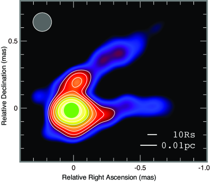
Figure 1.— The one-zone sphere region treated in this work (the yellow-green colored circle) overlayed on the actual VLBA image of M87 at 43 GHz. While the limb-brightening structure is seen at the outer part, the central region of the radio core can be approximately described as a uniform sphere. The diameter of this yellow-green circle corresponds to $\theta_{\rm FWHM}=0.11~{}{\rm mas}$. Details of the 43 GHz image have been explained in H13.

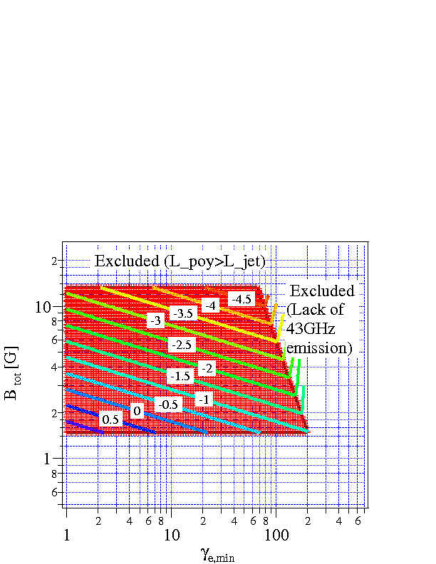
Figure 2.— The allowed region in $\gamma_{e,\rm min}$ and $B_{\rm tot}$ plane (the red-colored boxed region) and the corresponding $\log(U_{e}/U_{B})$ values with $L_{\rm jet}=5\times 10^{44}~{}{\rm ergs^{-1}}$ and $p=3.0$. The $\log(U_{e}/U_{B})$ value is obtained from Eq. (14). The boundary of the allowed region is determined by Eqs. (15), (3.3), and (27). (Short stray lines from the box should be ignored.)

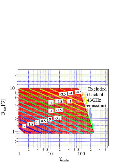
Figure 3.— Same as Fig. (2) but with $p=3.5$.

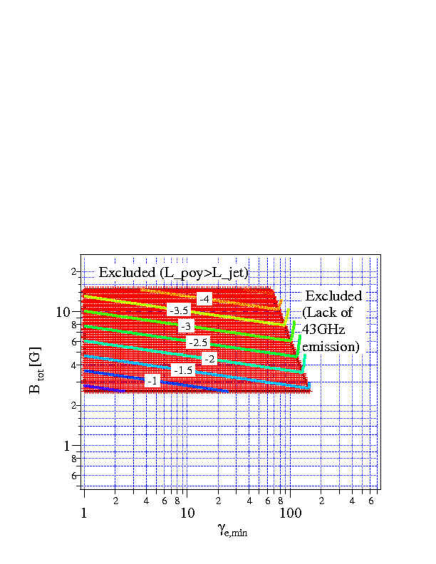
Figure 4.— Same as Fig. (2) but with $p=2.5$.

Table 1Relevant coefficients for $B$ and $K_{e}$

$p$	$c_{1}(p)$	$c_{2}(p)$	$b(p)$	$b(p)$ by Hirotani (2005)	$b(p)$ by Marscher (1983)	$k(p)$
2.5	1.516	0.405	$3.3\times 10^{-5}$	$2.36\times 10^{-5}$	$3.6\times 10^{-5}$	$1.4\times 10^{-2}$
3.0	1.490	0.303	$1.9\times 10^{-5}$	$2.08\times 10^{-5}$	$3.8\times 10^{-5}$	$2.3\times 10^{-3}$
3.5	1.520	0.245	$1.2\times 10^{-5}$	$1.78\times 10^{-5}$	–	$3.6\times 10^{-4}$

Table 2Allowed $B_{\rm tot}$ and $\theta_{\rm obs}$

$p$	$L_{\rm j}$	minimum $B_{\rm tot}$	maximum $B_{\rm tot}$	minimum $\theta_{\rm obs}$	maximum $\theta_{\rm obs}$
	[erg s-1]	[G]	[G]	[G]	[mas]
2.5	$1\times 10^{44}$	2.5	7.7	0.11	0.15
2.5	$5\times 10^{44}$	2.5	14.7	0.11	0.17
3.0	$1\times 10^{44}$	1.5	6.9	0.11	0.16
3.0	$5\times 10^{44}$	1.5	13.3	0.11	0.19
3.5	$1\times 10^{44}$	0.93	6.3	0.11	0.18
3.5	$5\times 10^{44}$	0.93	9.6	0.11	0.20

Table 3Obtained maximum and minimum $U_{e}/U_{B}$

$p$	$L_{\rm j}~{}{\rm[erg~{}s^{-1}]}$	$\max U_{e}/U_{B}$	$\min U_{e}/U_{B}$
2.5	$1\times 10^{44}$	$0.5$	$3.6\times 10^{-4}$
2.5	$5\times 10^{44}$	$0.5$	$2.4\times 10^{-5}$
3.0	$1\times 10^{44}$	$22$	$1.6\times 10^{-4}$
3.0	$5\times 10^{44}$	$22$	$1.0\times 10^{-5}$
3.5	$1\times 10^{44}$	$1.2\times 10^{2}$	$0.9\times 10^{-4}$
3.5	$5\times 10^{44}$	$6.1\times 10^{2}$	$1.3\times 10^{-5}$

References

- Abdo et al. (2009) Abdo, A. A., Ackermann, M., Ajello, M., et al. 2009, ApJ, 707, 55
- Abramowski et al. (2012) Abramowski, A., Acero, F., Aharonian, F., et al. 2012, ApJ, 746, 151
- Acciari et al. (2009) Acciari, V. A., et al. 2009, Sci, 325, 444
- Asada et al. (2014) Asada, K., Nakamura, M., Doi, A., Nagai, H., & Inoue, M. 2014, ApJ, 781, L2
- Asada et al. (2009) Asada, K., Doi, A., Kino, M., et al. 2009, Approaching Micro-Arcsecond Resolution with VSOP-2: Astrophysics and Technologies, 402, 262
- Asano & Takahara (2009) Asano, K., & Takahara, F. 2009, ApJ, 690, L81
- Bardeen & Petterson (1975) Bardeen, J. M., & Petterson, J. A. 1975, ApJ, 195, L65
- Bicknell & Begelman (1996) Bicknell, G. V., & Begelman, M. C. 1996, ApJ, 467, 597
- Blandford & Rees (1978) Blandford, R. D., & Rees, M. J. 1978, Phys. Scr, 17, 265
- Blandford & Znajek (1977) Blandford, R. D., & Znajek, R. L. 1977, MNRAS, 179, 433
- Blumenthal & Gould (1970) Blumenthal, G. R., & Gould, R. J. 1970, Reviews of Modern Physics, 42, 237 (BG70)
- Boldt & Loewenstein (2000) Boldt, E., & Loewenstein, M. 2000, MNRAS, 316, L29
- Broderick & Loeb (2009) Broderick, A. E., & Loeb, A. 2009, ApJ, 697, 1164
- Burbidge et al. (1974) Burbidge, G. R., Jones, T. W., & Odell, S. L. 1974, ApJ, 193, 43
- Dexter et al. (2012) Dexter, J., McKinney, J. C., & Agol, E. 2012, MNRAS, 421, 1517
- Dodson et al. (2013) Dodson, R., Rioja, M., Asaki, Y., et al. 2013, AJ, 145, 147
- Dodson et al. (2006) Dodson, R., Edwards, P. G., & Hirabayashi, H. 2006, PASJ, 58, 243
- Doeleman et al. (2012) Doeleman, S. S., Fish, V. L., Schenck, D. E., et al. 2012, Science, 338, 355
- Doi et al. (2013) Doi, A., Hada, K., Nagai, H., et al. 2013, The Innermost Regions of Relativistic Jets and Their Magnetic Fields, Granada, Spain, Edited by Jose L. Gomez; EPJ Web of Conferences, European Physical Journal Web of Conferences, 61, 8008
- Doi et al. (2006) Doi, A., Nagai, H., Asada, K., et al. 2006, PASJ, 58, 829
- Gebhardt & Thomas (2009) Gebhardt, K., & Thomas, J. 2009, ApJ, 700, 1690
- Ginzburg & Syrovatskii (1965) Ginzburg, V. L., & Syrovatskii, S. I. 1965, ARA&A, 3, 297 (GS65)
- Hada (2013) Hada, K. 2013b, The Innermost Regions of Relativistic Jets and Their Magnetic Fields, Granada, Spain, Edited by Jose L. Gomez; European Physical Journal Web of Conferences, 61, 1002
- Hada et al. (2013) Hada, K., Kino, M., Doi, A., et al. 2013a, ApJ, 775, 70 (H13)
- Hada et al. (2012) Hada, K., Kino, M., Nagai, H., et al. 2012, ApJ, 760, 52
- Hada et al. (2011) Hada, K., Doi, A., Kino, M., et al. 2011, Nature, 477, 185 (H11)
- Hatchett et al. (1981) Hatchett, S. P., Begelman, M. C., & Sarazin, C. L. 1981, ApJ, 247, 677
- Hirotani (2005) Hirotani, K. 2005, ApJ, 619, 73
- Iwamoto & Takahara (2002) Iwamoto, S., & Takahara, F. 2002, ApJ, 565, 163
- Jones et al. (1974) Jones, T. W., O’dell, S. L., & Stein, W. A. 1974a, ApJ, 192, 261
- Jones et al. (1974) Jones, T. W., O’dell, S. L., & Stein, W. A. 1974b, ApJ, 188, 353
- Jordán et al. (2005) Jordán, A., Côté, P., Blakeslee, J. P., et al. 2005, ApJ, 634, 1002
- Junor et al. (1999) Junor, W., Biretta, J. A., & Livio, M. 1999, Nature, 401, 891
- Kellermann & Pauliny-Toth (1969) Kellermann, K. I., & Pauliny-Toth, I. I. K. 1969, ApJ, 155, L71
- Kino et al. (2012) Kino, M., Kawakatu, N., & Takahara, F. 2012, ApJ, 751, 101
- Kino & Takahara (2004) Kino, M., & Takahara, F. 2004, MNRAS, 349, 336
- Kino et al. (2002) Kino, M., Takahara, F., & Kusunose, M. 2002, ApJ, 564, 97
- Koide et al. (2002) Koide, S., Shibata, K., Kudoh, T., & Meier, D. L. 2002, Science, 295, 1688
- Komissarov et al. (2009) Komissarov, S. S., Vlahakis, N., Konigl, A., & Barkov, M. V. 2009, MNRAS, 394, 1182
- Komissarov et al. (2007) Komissarov, S. S., Barkov, M. V., Vlahakis, N., Konigl, A. 2007, MNRAS, 380, 51
- Kovalev et al. (2007) Kovalev, Y. Y., Lister, M. L., Homan, D. C., & Kellermann, K. I. 2007, ApJ, 668, L27
- Krolik et al. (2005) Krolik, J. H., Hawley, J. F., & Hirose, S. 2005, ApJ, 622, 1008
- Krichbaum et al. (2006) Krichbaum, T. P., Graham, D. A., Bremer, M., et al. 2006, Journal of Physics Conference Series, 54, 328
- Krichbaum et al. (2005) Krichbaum, T. P., Zensus, J. A., & Witzel, A. 2005, AN, 326, 548
- Lähteenmäki et al. (1999) Lähteenmäki, A., Valtaoja, E., & Wiik, K. 1999, ApJ, 511, 112
- Ly et al. (2007) Ly, C., Walker, R. C., & Junor, W. 2007, ApJ, 660, 200
- Macchetto et al. (1997) Macchetto, F., Marconi, A., Axon, D. J., et al. 1997, ApJ, 489, 579
- Marscher (1987) Marscher, A. P. 1987, Superluminal Radio Sources, 280
- Marscher (1983) Marscher, A. P. 1983, ApJ, 264, 296 (M83)
- McKinney et al. (2013) McKinney, J. C., Tchekhovskoy, A., & Blandford, R. D. 2013, Science, 339, 49
- McKinney (2006) McKinney, J. C. 2006, MNRAS, 368, 1561
- McKinney & Gammie (2004) McKinney, J. C., & Gammie, C. F. 2004, ApJ, 611, 977
- Nagai et al. (2013) Nagai, H., Kino, M., Niinuma, K., et al. 2013, PASJ, 65, 24
- Nakamura & Asada (2013) Nakamura, M., & Asada, K. 2013, 775, 118
- Neronov & Aharonian (2007) Neronov, A., & Aharonian, F. A. 2007, ApJ, 671, 85
- Owen et al. (2000) Owen, F. N., Eilek, J. A., & Kassim, N. E. 2000, ApJ, 543, 611
- Pacholczyk (1970) Pacholczyk, A. G. 1970, Series of Books in Astronomy and Astrophysics, San Francisco: Freeman, 1970,
- Reynolds et al. (1996) Reynolds, C. S., Fabian, A. C., Celotti, A., & Rees, M. J. 1996, MNRAS, 283, 873
- Rieger & Aharonian (2012) Rieger, F. M., & Aharonian, F. 2012, Modern Physics Letters A, 27, 30030
- Rybicki & Lightman (1979) Rybicki, G. B., & Lightman, A. P. 1979, New York, Wiley-Interscience, 1979 (RL79)
- Stawarz et al. (2006) Stawarz, Ł., Kneiske, T. M., & Kataoka, J. 2006, ApJ, 637, 693
- Takahashi & Mineshige (2011) Takahashi, R., & Mineshige, S. 2011, ApJ, 729, 86
- Tchekhovskoy et al. (2011) Tchekhovskoy, A., Narayan, R., & McKinney, J. C. 2011, MNRAS, 418, L79
- Thorne et al. (1986) Thorne, K. S., Price, R. H., & MacDonald, D. A. 1986, Black Holes: The Membrane Paradigm, Yale University Press
- Toma & Takahara (2013) Toma, K., & Takahara, F. 2013, Progress of Theoretical and Experimental Physics, 2013, 080003
- Vlahakis Konigl (2003) Vlahakis, N., Konigl, A. 2003, ApJ, 596, 1080
- Walsh et al. (2013) Walsh, J. L., Barth, A. J., Ho, L. C., & Sarzi, M. 2013, ApJ, 770, 86
- Weinberg (1972) Weinberg, S. 1972, Gravitation and Cosmology: Principles and Applications of the General Theory of Relativity, ISBN 0-471-92567-5. Wiley-VCH