The tunneling model of laser-induced ionization and its failure at low frequencies
Abstract
The tunneling model of ionization applies only to longitudinal fields: quasistatic electric fields that do not propagate. Laser fields are transverse: plane wave fields that possess the ability to propagate. Although there is an approximate connection between the effects of longitudinal and transverse fields in a useful range of frequencies, that equivalence fails completely at very low frequencies. Insight into this breakdown is given by an examination of radiation pressure, which is a unique transverse-field effect whose relative importance increases rapidly as the frequency declines. Radiation pressure can be ascribed to photon momentum, which does not exist for longitudinal fields. Two major consequences are that the near-universal acceptance of a static electric field as the zero frequency limit of a laser field is not correct; and that the numerical solution of the dipole-approximate Schrödinger equation for laser effects is inapplicable as the frequency declines. These problems occur because the magnetic component of the laser field is very important at low frequencies, and hence the dipole approximation is not valid. Some experiments already exist that demonstrate the failure of tunneling concepts at low frequencies.
pacs:
32.80.Rm, 33.80.Rv, 42.50.Hz, 03.50.De7 May 2014]
I Introduction
The quantum phenomenon of tunneling through a potential barrier has been known and fruitfully employed since its introduction in 1928 to describe nuclear alpha decaygamow and, in the same year, to calculate the ionization of the hydrogen atom by a constant electric fieldoppie . Both of those early applications involved static electric fields. The same concept has been applied in more recent yearskeldysh ; n+r ; ppt to laser-induced ionization when the laser field is approximated as a quasistatic electric field. The concept of tunneling ionization is that an impenetrable potential barrier is rendered penetrable by the superposition of an oscillatory electric field: . It is usual to describe the applied field by a scalar potential,
| (1) |
since this leads to the familiar graphical illustration where a potential well representing the force binding an electron to an atom is periodically depressed to allow the electron to escape by tunneling through the depressed barrier. The potentials in Eq.(1) describe a longitudinal field. Longitudinal fields can oscillate in time, but they do not propagate. The scalar-potential-only nature of Eq.(1) is usual but not essential. It is always possible to find a gauge transformation that replaces the scalar potential in Eq.(1) by a vector potential . Gauge equivalence means that such a vector-potential description also represents a longitudinal field.
Actual laser fields are true propagating plane-wave (PW) fields, also known as transverse fields. The name comes from the fact that a PW field has electric and magnetic components of equal magnitude (in Gaussian units) that are perpendicular to each other, and the plane they define is perpendicular to the direction of propagation. That is, propagation is in a direction transverse to the electric and magnetic fields. Laser fields are vector fields that cannot be completely described by a scalar potential, nor by any potential that is gauge-equivalent to a scalar potential. The simplest way to describe transverse fields (see, for example, the textbook of Jacksonjackson ) is by a vector potential function alone
| (2) |
that depends on spacetime coordinates only in the combination
| (3) | ||||
| (4) |
The quantity is the phase of a propagating field, and and are the 4-vector propagation vector and its 3-vector component. This prescription for the potentials is known as the radiation gauge (or Coulomb gauge).
Longitudinal and transverse fields are fundamentally different electromagnetic phenomena. These differences are explored in depth in this article.
For some purposes it is possible to neglect the dependence of on the spatial coordinate , in which case (known as the dipole approximation) there is a gauge transformation due to Göppert-Mayergm (GM) that provides a gauge equivalence between the dipole-approximation vector potential and the scalar potential of Eq.(1). It is of fundamental importance to maintain awareness that fields described within the GM gauge (also known as the length gauge) cannot be anything more than longitudinal fields. A longitudinal field can never be gauge-equivalent to a transverse field, but only to an approximation to a transverse field. This means that the tunneling concept, dependent on the scalar potential (1) or any potential gauge-equivalent to (1), can never be more than a limited approximation for laser phenomena. It is the elucidation of these limitations that is a major focus of this article.
Tunneling is a concept applicable only to longitudinal fields, and is only a very limited approximation for transverse (e.g. laser) fields. The focus of attention is now shifted to an examination of parameters wherein tunneling can be a meaningful approximation for laser fields.
There is an upper limit on the field frequency for which the dipole approximation is applicable that was pointed out by Göppert-Mayergm . When the field wavelength is less than the size of the atom, it can act as a probe of the structure of the atom. That is not possible for , which limits the field frequency to
| (5) |
in atomic units.
It is not generally recognized that there is a lower limit to the frequency at which the dipole approximation can be applied. This lower limit is of far more practical importance than the upper limit of Eq.(5). The reason for this oversight may be that no such lower limit exists for QSE fields but, importantly, it does for PW fields
Section II gives a qualitative insight into the atomic domain as it appears for QSE fields; that is for fields describable by Eq.(1), and Section III repeats the analysis for PW fields. The contrast between the two types of fields is striking. This comes about because the strength of a longitudinal field is judged only by the magnitude of the electric field, whereas it is the strongly frequency-dependent ponderomotive potential that is required for appraisal of transverse fieldshr62b ; hr89 . For instance, a parameter domain that applies to very weak QSE fields is shown to consist of very strong PW fields, and vice versa. Important matters elaborated in Section III include the criteria for the onset of nondipole effects at low frequencies. Section IV concentrates explicitly on low-frequency behavior.
The analytical methods available for the description of ionization by strong laser fields are described in Section V. These include the tunneling model, the strong-field approximation (SFA), and the numerical solution of the time-dependent Schrödinger equation (TDSE). The domains of applicability have some overlap, but this overlap is far more limited than is evident from the current literature. In particular, the literature exhibits widespread dependence on the “exactness” of the TDSE without regard for the failure of the dipole approximation for low-frequency laser fields.
Finally, the results are summarized and evaluated in Section VI. Qualitative assessments are made, including the conclusion that the tunneling approximation is useful for laser-induced ionization problems in only a very small region in the frequency and intensity domain of laser fields.
II Quasistatic electric fields
The simplest electromagnetic field is a static electric field. This can be described by the potentials
| (6) |
where the subscript on the electric field vector is a reminder that the field so described is constant. A simple but important generalization is a field configuration in which there is no magnetic field and the electric field is time-dependent, as in Eq.(1). This a quasistatic electric (QSE) field. Another indicator of this identification is the Lorentz invariant
| (7) |
where the inner product of the two electromagnetic-field tensors on the right-hand side of the equation shows the reason why this quantity is a Lorentz scalar; that is, its value is invariant under any Lorentz transformation. For QSE fields, it is always true that
| (8) |
By contrast, a laser field is a PW field for which it is always true that
| (9) |
The important conclusion is that the GM gauge, that employs the potentials (1) (or any potentials gauge-equivalent to (1)) for the description of a laser field, approximates the laser field by a QSE field. There is no limit in which the GM gauge is exact.
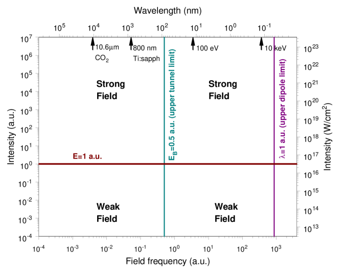
A QSE field is a longitudinal field, which means that there is only one spatial direction that is important: the electric field direction. A QSE field does not possess a propagation capability; it can oscillate with time, but it cannot propagate. The electromagnetic field enters into the potentials through the direction and the magnitude of the electric field. In atomic applications, the electric field is strong when , and it is weak when This is indicated in Fig. 1, which is a plot showing field frequency on the and field intensity on the . Intrinsic frequency considerations do not occur, but two frequency limits of atomic origin are shown. One is the well-known upper limit on the dipole approximation, where Fig.1 shows the frequency that is given in Eq.(5). Another upper limitation on the frequency comes from the tunneling method itself, since tunneling is only meaningful when an uncountably large number of photons participate. In practical terms, “uncountably large” in an ionization event may be satisfied by a number of the order of . Figure 1 shows this tunneling limit in terms of the binding energy of an electron in ground-state hydrogen at
Among the qualitative properties just listed about QSE fields, there is nothing to serve as an indicator that the dipole approximation is inapplicable to laser fields at low frequencies. This is apparently the underlying reason why a low-frequency limit has escaped notice in the Atomic, Molecular, and Optical (AMO) community. Even a modern book entitled Atoms in Intense Laser Fieldsjkp asserts (see pp.267-289) that the GM gauge is the preferred gauge for laser problems since it is well-behaved as the frequency approaches zero. There is no awareness that there is a low-frequency limit for the applicability of the GM gauge to laser problems. The line of reasoning followed by the authors is based on the concept of adiabaticity, and the entire discussion depends on the validity of the dipole approximation. The fact that a constant electric field emerges as is prima facie evidence that the discussion in Ref.jkp relates only to longitudinal fields and not to laser fields.
Another clear indication of the problem that exists in the AMO community can be found in a recent paper in a prestigious rapid-publication journal, where two consecutive sentences that are contradictory are viewed as if they were mutually supportivearissian . The first sentence is: “In adiabatic tunneling the laser field is treated as if it were a static field, time serving only as a parameter.” That is, the authors state that they are treating the laser field as if it were a QSE field, where Eq.(8) is valid. The next sentence is: “It is rigorously valid for long wavelengths …” The authors thereby state that they view the laser field as if it has a zero-frequency limit, and they view that limit as a static electric field, despite the previous statement that they are concerned with laser fields, where Eq.(9) applies. Equations (8) and (9) are incompatible, not equivalent. References jkp and arissian are not singled out for special criticism, but they are cited because they are especially visible representations of the prevailing view.
The following Section further elaborates the fundamental differences between QSE fields and laser fields.
III Plane wave fields
Plane wave (PW) fields are transverse fields. (See Chapter 7 in the text by Jacksonjackson .) An essential property of PW fields is that any occurrence of the spacetime 4-vector must occur as the scalar product with the propagation 4-vector schwinger ; s+s ; hrjmo , as shown in Eq.(3). This product, which is the phase of a propagating field, will be called . The descriptions “PW”, “transverse”, and “propagating” are here viewed as equivalent designations of the type of fields that lasers produce. A basic property of such fields is that, once generated, they propagate indefinitely in vacuum without the need for sources.
This last property is very important. The GM gauge does not have that feature of a freedom from sources. That is, no field can exist in the GM gauge without sources to sustain ithrjpb13 . They are “virtual sources” in the sense that they do not actually exist in the laboratory. Because of the gauge equivalence between the GM gauge and a dipole approximation to a PW, the properties of those sources do not normally intrude in a calculation. There are special cases, however, when the virtual sources of the GM gauge can produce unintended consequenceshrjpb13 even when the dipole approximation is valid.
The best indicator of the strength of coupling of a PW field to a charged particle is the ponderomotive potential given by
| (10) |
in atomic units, where is the field intensity. In the radiation gauge, this quantity is a true potential energyhr89 that depends on the local values of and . Its dimensionless form also serves as the coupling constant between a strong PW field and an electron, replacing the fine structure constant of perturbation theoryhr62a ; hr62b ; hr89 . The analog of in the GM gauge is a “quiver energy” that corresponds to the oscillation of the charged particle as it is driven by the QSE field. The magnitude of is the same in both gauges, but the interpretation is different. In the GM gauge, is a kinetic energy of the charged particle that results from the virtual sources described above. In the radiation gauge, there are no sources to drive the particle, and is a potential energy, not a kinetic energy.
In the nonperturbative theory of the interaction of charged free particles with strong laser fields, as in Compton scatteringsengupta , photon-multiphoton pair productionhr62a , or pair annihilationn+r64 , a single intensity parameter occurs that is the same for all free-particle interactions. Many different notations occur in the literature, but it will be designated here as , where
| (11) |
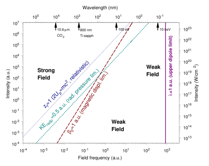
The quantity can be viewed as a dimensionless statement of the ponderomotive potential. When , then equals the rest energy of the particle, and the process is unequivocally relativistic. This means that the dipole approximation has no validity. Figure 2 is the PW analog of Fig.1 for QSE fields, and the line corresponding to shows immediately that there is a drastic difference between the behavior of QSE and PW fields. For example, the lower left region of Fig.1 corresponds to a very weak QSE field, whereas the same region in Fig.2 represents a very strong PW field. The line corresponding to is given by
| (12) |
in atomic units.
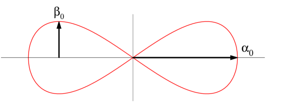
The condition refers to a strongly relativistic environment, but the onset of nondipole behavior can occur at significantly lower intensities. One way to estimate the lower-frequency limit of the dipole approximation is to examine the well-known “figure-8” motion of a free charged particle in a PW fieldl+l ; s+s . This is shown in Fig.3 in the frame of reference where the particle is at rest when averaged over a full cycle. At low field intensity, the figure-8 reduces to a straight-line oscillation of amplitude . Departure from straight-line behavior occurs at increasing intensity since the coupled action of the electric and magnetic fields of the PW causes a motion in the direction of propagation of the field. When the amplitude in the propagation direction is of the order of one atomic unit,
| (13) |
this signals an important contribution from the magnetic field that will certainly influence the nature of the interaction with the ion, and the dipole approximation is not valid. The line determined by the condition (13) is
| (14) |
in atomic units, and is shown in Fig.2.
An alternative way to assess the importance of nondipole effects is to consider the momentum and energy of a motion induced by radiation pressure. The momentum in the direction of field propagation resulting from radiation pressure ishrrel ; t+d ; hr87
| (15) |
The kinetic energy corresponding to this momentum is
| (16) |
where the nonrelativistic form on the left-hand side is sufficient since this limitation occurs well before the fully relativistic limit is reached at The condition (16) gives the line in Fig.2 determined by
| (17) |
in atomic units. This is parallel to the of Eq.(12), but smaller by the factor a.u. That is, the onset of a relativistic effect like radiation pressure makes its presence felt well before the fully relativistic condition of Eq.(12).
By using very sensitive measurement techniques, radiation pressure effects have already been observed in the laboratorysmeenk at 800 nm wavelength. An intensity of was specifically analyzedt+d ; hr87 . In atomic units, the intensity was , whereas Eq.(17) predicts for that wavelength. Thus the experiment detected radiation pressure at little more than one percent of the condition stated in Eq.(17). This confirms that Eq.(17) gives a realistic assessment of conditions where the dipole approximation will fail.
IV Low Frequencies
Figures 1 and 2 make it very clear that longitudinal fields and transverse fields are different electromagnetic phenomena. That major distinction arises from the unique properties of a propagating field. The failure of correspondence is most striking at low frequencies. From the point of view of longitudinal fields, low frequencies are viewed as being in the so-called tunneling limit, where QSE fields approach static electric fields. For transverse fields, low frequencies correspond to the completely different domain of Extreme Low Frequency (ELF) radio waves. The qualitative features of these two fundamentally different domains of electromagnetic phenomena are outlined here.
IV.1 “Tunneling limit” and the Keldysh parameter
The tunneling view of ionization leads to a single controlling intensity parameter known as the Keldysh parameterkeldysh that can be written as
| (18) |
where is the binding energy of the electron in the atom or molecule. This quantity is also called the ionization potential, and designated by or . The putative tunneling domain is defined by
| (19) |
and the tunneling limit is
| (20) |
The opposite case to the tunneling domain is the so-called multiphoton domain: . It has become standard practice in the description of laser-induced processes to specify whether an experiment or theory relates to one or the other of these two longitudinal-field domains, without regard to the qualitatively different behavior of actual laser (transverse) fields.
With Eq.(10) used to introduce field intensity and frequency into Eq.(18), the dividing line between these two domains will be called , and is given by
| (21) |
which leads to the tunneling limit expressed as . Equation (21) has the same dependence as in Eq.(12) and in Eq.(17), although the prefactors are such that lies well below the other two lines in a diagram such as Fig.2. As the frequency declines, however, the physical system heads inexorably towards the relativistic domain where the dipole approximation certainly fails and the tunneling approximation has no applicability to laser effectshr82 . On the other hand, from the point of view of longitudinal fields, declining frequency is simply a matter of an ac field approaching a dc limit. This appears to present no conceptual problemsshakeshaft , and the AMO community routinely evaluates analytical methods by the limit as . If that limit corresponds to static-electric-field results, this is regarded as evidence of an acceptable theory. The fact that for such a limit seems never to be noticed.
IV.2 ELF radio waves
Transverse fields always retain their propagation property as meaning that is sustained and the magnetic field is always present. Maintenance of the propagation property means that decreasing frequency implies a progression from ultraviolet to visible to infrared to microwave to radio phenomena. The zero frequency limit can be approached, but never reached. The divergence of as , shown in Eq.(10), is symptomatic of the energy demands of producing ELF radio transmissions. The lowest ELF frequency of which this writer is aware is the system that the U.S. Navy proposed as a means of communicating with submerged submarines. The project was named “Project Sanguine”sanguine , and the original design (never built) required a massive of power to produce a signal with such small bandwidth that only simple coded messages could be sent.
An ELF radio wave is conceptually as distant from a constant electric field as would be a pure magnetic field when judged by the relevant value. Nevertheless, the hallmark of success valued from a QSE point of view in the AMO community is that theoretical predictions should match the properties of constant electric fields. This is completely inappropriate for laser fields.
V Analytical methods
A brief survey is given here of some of the consequences of the foregoing considerations for theoretical techniques employed to describe atomic systems subjected to very intense laser fields.
V.1 Tunneling
Time-independent potential barriers that are penetrable by quantum tunneling processes are treated in essentially all textbooks on quantum mechanics, and that problem is thoroughly understood. Tunneling methods were later applied to QSE fieldskeldysh ; n+r ; ppt . Many investigators who depend on tunneling methods to solve problems in laser-induced ionization processes regard the existence of a static-field limit of their method as a reassurance of accuracy. This should be worrisome rather than reassuring. Transverse fields do not have a physically attainable zero frequency limit, which is evident in several ways. The radiation pressure result would be divergent were there a zero frequency limit, as is clear from Eqs.(15) and (10). Figure 2 shows that there is no access to zero frequency of a PW field without entering into the relativistic domain where the dipole approximation necessarily fails. Under relativistic conditions the magnetic component of a transverse field becomes as important as the electric component. Theories of relativistic tunneling have been publishedkmp , but they relate only to extremely strong QSE fields. Relativistically strong laser fields cannot be treated by QSE methods.
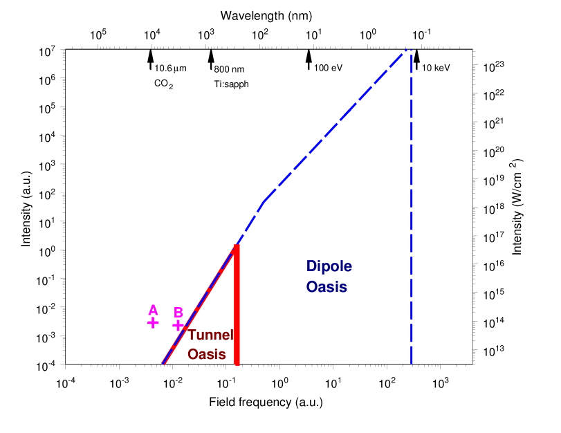
Figure 4 shows the domain in an intensity-frequency diagram where the tunneling method is applicable for laser-induced processes. This domain is dubbed the “Tunnel Oasis”, since that is where a tunneling model can be applied successfully without concern for the broader limitations of the tunneling approximation. The lower limits on frequency come entirely from transverse-field effects as shown in Fig.2. Such effects are not present in a longitudinal-field analysis, as Fig.1 clearly shows. The upper limit on frequency is specific to tunneling, since the basic premise of a tunneling theory is that it is a field-emission effect, not explicable in terms of a limited number of photons.
Experiments done with a laser in the 1980slaval showed a striking departure from the properties of tunneling behaviorhr102 . The -laser parameters are shown as the point labeled “” in Fig.4. This is plainly outside the Tunnel Oasis. The pioneering “low-energy-structure” (LES) experimentsosu1 ; osu2 of the group at Ohio State University also possess spectrum features that are not explicable within the tunneling approximation, which is to be expected from the location marked “” in Fig.4. Both of these sets of experiments with linearly polarized light show clear departures from tunneling behavior, where the spectrum peaks sharply at zero energycbb ; dk .
A remarkable feature of the Tunnel Oasis is how small it is when compared to the overall parameter space which is, or will become, the range of laser parameters. One may call it an “accident of Nature” that the most commonly used source of strong laser fields operates at about , within the Oasis except at extremely large intensities where saturation will occur, and the failure of the tunneling model is obscured.
Another aspect of Fig.4 is that the lowest intensity shown is (). Traditional AMO physics is conducted at much lower intensities than that, where the triangular Tunnel Oasis expands considerably. This is the underlying reason why the limitations of the GM gauge and its low-frequency failure have not become visible until recently.
V.2 Strong-Field Approximation
The Strong-Field Approximation (SFA) is based on the idea that after a photoelectron has been ionized from an atom by a very intense field, its behavior is dominated by the field that caused the ionization, rather than by the residual effects of the binding potentialhr80 . Discussion of the SFA is difficult because its definition has become muddled. The analytical approximation method of Ref.hr80 is not a tunneling method, so the name “Strong-Field Approximation” was proposedhr90 for this method to distinguish it from GM-gauge methods that are all basically tunneling approximations. Unfortunately, the purpose of Ref.hr90 was not understood, and so the designation “SFA” began to be applied to all approximations where the field in the final state dominates residual Coulomb effects.
The remarks that follow pertain only to the non-tunneling SFA of 1980hr80 . The 1990 paperhr90 showed that the method of Ref.hr80 is actually based on a completely relativistic formalism, when that can be subjected to the dipole approximation. The distinction that is vital is that the magnetic field is always present but, apart from the essential propagation property it imparts, its direct effect can otherwise be ignored when nonrelativistic conditions obtain. This confines the 1980 SFA to the portion of Fig.4 labeled “Dipole Oasis”, but not to the much smaller Tunnel Oasis. (Actually, the SFA appears to retain some of its relativistic character even into the low-frequency domain below the Tunnel Oasishr102 .) This equivalence to a full transverse-field approximation was demonstrated explicitly in another paper, also in 1990hrrel , by a completely relativistic calculation that reduced in the nonrelativistic case to the 1980 SFA directly with no resort to any tunneling-type approximations. The applicability of the 1980 SFA to domains outside the Tunnel Oasis, but within the Dipole Oasis has been verified by successful high frequency comparisons with the TDSEbondar and with the High-Frequency Approximation (HFA) of Gavrilahrjosa96 .
V.3 Time-Dependent Schrödinger Equation
Direct numerical solution of the time-dependent Schrödinger equation for laser-induced processes has come to be called “TDSE”. Numerical methods have advanced to the point that accurate TDSE calculations can be performed over a wide range of laboratory parameters. TDSE is regarded as “exact”, and it is frequently applied to verify the accuracy of analytical approximations. A disadvantage of TDSE is that it does not give clear physical insights as to why particular types of behavior occur in physical systems, whereas analytical approximations can give rise to instructive physical interpretations.
The perception of exactness of the TDSE approach has been carried too far. Many investigators (see, for example, Ref.jkp ) fail to notice the low-frequency limit of the dipole approximation, and make the assumption that TDSE can comfortably be extended all the way to zero frequency. The range of applicability of the TDSE numerical method is indicated by the Dipole Oasis domain in Fig.4. Numerical methods applied to frequencies lower than the Dipole Oasis would require eschewing the dipole approximation for frequencies somewhat less than the low frequency limit of the Tunnel Oasis, and full solution of the Dirac equation in three spatial coordinates for still lower frequencies. Those capabilities do not exist at present.
V.4 Length gauge and velocity gauge
The meaning of “length gauge” is unambiguous: it is identical to the GM gauge. That is, it refers to the representation of an electromagnetic field of laser origin by the scalar potential of Eq.(1). In other words, it approximates a PW field by the conceptually simpler QSE field.
The term “velocity gauge” can be misinterpreted, as detailed in the above discussion about the SFA. The simplest solution to this situation is to confine the meaning of velocity gauge to that use of the dipole approximation that is exactly gauge-equivalent to the GM (or length) gauge. The basic interaction Hamiltonian for the velocity gauge is, in atomic units and for a single particle:
| (22) |
VI Summary
For a charged particle in a laser field (or in any propagating field), it is at low frequencies that the magnetic component of the field becomes most important. This stands in sharp contrast to charged particle behavior in any field describable by a scalar potential of the form (a longitudinal field) for which no magnetic field exists. The tunneling model of ionization is confined entirely to longitudinal fields, so it has no relevance for low-frequency laser fields.
Quality indices based on the potential are actually counter-indicative. A frequently-employed example is the concept that an analytical method should reproduce static-electric-field properties as the frequency declines. This violates the very concept of a propagating field that, to maintain its propagation property, must always retain the appropriate time dependence given by the phase of the propagating field.
The low-frequency failure of dipole-approximation methods applies to all such techniques employed for laser fields, including numerical methods for solution of the Schrödinger equation (TDSE) and all length-gauge and velocity-gauge treatments. The tunneling model is a length-gauge approximation that has the additional limitation imposed by the high-frequency constraint that the energy of a single photon of the field must be much less than the binding potential of a prospective detached electron. The result is that the “Tunnel Oasis” of Fig.4, defining the domain of laser parameters for which the tunneling model can be applied, is far smaller than the overall “Dipole Oasis” in Fig.4 within which the dipole approximation for laser-field effects has validity.
The Oases shown in Fig.4 continue to expand as the intensity falls below the lowest intensity of the figure. Traditional AMO physics is conducted at much lower intensities where the low-frequency failures of the GM gauge and of the tunneling model are not in evidence. This is the most likely explanation for why the low-frequency failure of the dipole approximation has not previously attracted notice. That situation is changing.
Existing laser experiments at low frequencies already show the failure of the tunneling approximation.
References
- (1) Gamow G 1928 Z. Physik 51 204-212
- (2) Oppenheimer J R 1928 Phys. Rev. 31 66-81
- (3) Keldysh L V 1965 Sov. Phys.–JETP 20 1307-14
- (4) Nikishov A I and Ritus V I 1966 Sov. Phys.–JETP 23 168-177
- (5) Perelomov A M, Popov V S and Terent’ev M V 1966 Sov. Phys.–JETP 23 924-934
- (6) Jackson J D 1975 Classical Electrodynamics 2nd edn (New York: Wiley)
- (7) Göppert-Mayer M 1931 Ann. Phys., Lpz. 9 273-94
- (8) Reiss H R 1962 J. Math. Phys. 3 387-395
- (9) Reiss H R 2014 Phys. Rev. A 89 022116
- (10) Joachain C J, Kylstra N J and Potvliege R M 2012 Atoms in Intense Laser Fields (Cambridge: Cambridge)
- (11) Arissian L, Smeenk C, Turner F, Trallero C, Sokolov A V, Villeneuve D M, Staudte A and Corkum P B 2010 Phys. Rev. Lett. 105 133002
- (12) Schwinger J 1951 Phys. Rev. 82 664-79
- (13) Sarachik E S and Schappert G T 1970 Phys. Rev. D 1 2738-53
- (14) Reiss H R 2012 J. Mod. Opt. 59 1371-1383; 2013 60 687
- (15) Reiss H R 2013 J. Phys. B: At. Mol. Opt. Phys. 46 175601
- (16) Reiss H R 1962 J. Math. Phys. 3 59-67
- (17) Sengupta N D 1952 Bull. Math. Soc. (Calcutta) 44 175-80
- (18) Nikishov A I and Ritus V I 1964 Sov. Phys.–JETP 19 529
- (19) Landau L D and Lifshitz E M 1975 The Classical Theory of Fields (Oxford: Pergamon)
- (20) Reiss H R 1990 J. Opt. Soc. Am. B 7 574-86
- (21) Titi A S and Drake G W F 2012 Phys. Rev. A 85 041404(R)
- (22) Reiss H R 2013 Phys. Rev. A 87 033421
- (23) Smeenk C T L, Arissian L, Zhou B, Mysyrowicz A, Villenueve D M, Staudte A and Corkum P B 2011 Phys. Rev. Lett. 106 193002
- (24) Reiss H R 2010 Phys. Rev. A 82 023418
- (25) Shakeshaft R, Potvliege R M, Dörr M and Cooke W E 1990 Phys. Rev. A 42 1656-1668
- (26) http://en.wikipedia.org/wiki/Project_Sanguine
- (27) Popov V S, Karnakov B M and Mur V D 2004 JETP Letters 79 262-7
- (28) Xiong W, Yergeau F, Chin S L and Lavigne P 1988 J. Phys. B: At. Mol. Opt. Phys. 21 L159-64
- (29) Reiss H R 2009 Phys. Rev. Lett. 102 143003
- (30) Colosimo P, Duomy G, Blaga C I, Wheeler J, Haury C, et al. 2008 Nat. Phys. 4 386-9
- (31) Blaga C I, Catoire F, Colosimo P, Paulus G G, Muller H G, Agostini P and DiMauro L F 2009 Nat. Phys. 5 335-8
- (32) Corkum P B, Burnett N H and Brunel F 1989 Phys. Rev. Lett. 62 1259-1262
- (33) Delone N B and Krainov V P 1991 J. Opt. Soc. Am. B 8 1207-1211
- (34) Reiss H R 1980 Phys. Rev. A 22 1786-1813
- (35) Reiss H R 1990 Phys. Rev. A 42 1476-1486
- (36) Bondar D I, Spanner M, Liu W K and Yudin G L 2009 Physical Review A 79 063404
- (37) Reiss H R 1996 J. Opt. Soc. Am. B 13 355-362
- (38) Reiss H R 1992 Prog. Quantum Electron. 16 1-71
- (39) Crawford D P 1994 PhD Dissertation: Relativistic Ionization with Intense Linearly Polarized Light (Washington, DC: American University)