Observations and three-dimensional photoionization modelling of the Wolf–Rayet planetary nebula Abell 48

Abstract

Recent observations reveal that the central star of the planetary nebula Abell 48 exhibits spectral features similar to massive nitrogen-sequence Wolf–Rayet stars. This raises a pertinent question, whether it is still a planetary nebula or rather a ring nebula of a massive star. In this study, we have constructed a three-dimensional photoionization model of Abell 48, constrained by our new optical integral field spectroscopy. An analysis of the spatially resolved velocity distributions allowed us to constrain the geometry of Abell 48. We used the collisionally excited lines to obtain the nebular physical conditions and ionic abundances of nitrogen, oxygen, neon, sulphur and argon, relative to hydrogen. We also determined helium temperatures and ionic abundances of helium and carbon from the optical recombination lines. We obtained a good fit to the observations for most of the emission-line fluxes in our photoionization model. The ionic abundances deduced from our model are in decent agreement with those derived by the empirical analysis. However, we notice obvious discrepancies between helium temperatures derived from the model and the empirical analysis, as overestimated by our model. This could be due to the presence of a small fraction of cold metal-rich structures, which were not included in our model. It is found that the observed nebular line fluxes were best reproduced by using a hydrogen-deficient expanding model atmosphere as the ionizing source with an effective temperature of $T_{\rm eff}$ = 70 kK and a stellar luminosity of $L_{\rm\star}$ = 5500 L_⨀, which corresponds to a relatively low-mass progenitor star ($\sim 3$ M_⨀) rather than a massive Pop I star.

1 Introduction

The highly reddened planetary nebula Abell 48 (PN G029.0$+$00.4) and its central star (CS) have been the subject of recent spectroscopic studies (Wachter et al., 2010; Depew et al., 2011; Todt et al., 2013; Frew et al., 2013). The CS of Abell 48 has been classified as Wolf–Rayet [WN5] (Todt et al., 2013), where the square brackets distinguish it from the massive WN stars. Abell 48 was first identified as a planetary nebula (PN) by Abell (1955). However, its nature remains a source of controversy whether it is a massive ring nebula or a PN as previously identified. Recently, Wachter et al. (2010) described it as a spectral type of WN6 with a surrounding ring nebula. But, Todt et al. (2013) concluded from spectral analysis of the CS and the surrounding nebula that Abell 48 is rather a PN with a low-mass CS than a massive (Pop I) WN star. Previously, Todt et al. (2010) also associated the CS of PB 8 with [WN/C] class. Furthermore, IC 4663 is another PN found to possess a [WN] star (Miszalski et al., 2012).

A narrow-band H$\alpha$+[N ii] image of Abell 48 obtained by Jewitt et al. (1986) first showed its faint double-ring morphology. Zuckerman & Aller (1986) identified it as a member of the elliptical morphological class. The H$\alpha$ image obtained from the SuperCOSMOS Sky H$\alpha$ Survey (Parker et al., 2005) shows that the angular dimensions of the shell are about 46$\hbox{${}^{\prime\prime}$}\times$ 38^′′, and are used throughout this paper. The first integral field spectroscopy of Abell 48 shows the same structure in the H$\alpha$ emission-line profile. But, a pair of bright point-symmetric regions is seen in [N ii] (see Fig. 2), which could be because of the N⁺ stratification layer produced by the photoionization process. A detailed study of the kinematic and ionization structure has not yet been carried out to date. This could be due to the absence of spatially resolved observations.

Table 1: Journal of the IFU observations with the ANU 2.3-m Telescope.

PN	Date (ut)	$\lambda$ range (Å)	$R$	Exp.(s)
Abell 48	2010/04/22	4415–5589	7000	1200
		5222–7070	7000	1200
	2012/08/23	3295–5906	3000	1200
		5462–9326	3000	1200

The main aim of this study is to investigate whether the [WN] model atmosphere from Todt et al. (2013) of a low-mass star can reproduce the ionization structure of a PN with the features like Abell 48. We present integral field unit (IFU) observations and a three-dimensional photoionization model of the ionized gas in Abell 48. The paper is organized as follows. Section 2 presents our new observational data. In Section 3 we describe the morpho-kinematic structure, followed by an empirical analysis in Section 4. We describe our photoionization model and the derived results in Sections 5 and 6, respectively. Our final conclusion is stated in Section 7.

2 Observations and data reduction

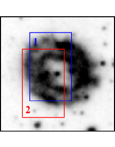
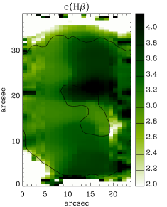
(a)                                 (b)

Figure 1: From left to right: (a) narrow-band filter image of PN Abell 48 in H$\alpha$ obtained from the SuperCOSMOS Sky H$\alpha$ Survey (SHS; Parker et al., 2005). The rectangles correspond the $25\times 38$-arcsec² IFU: 1 (blue) and 2 (red) taken in 2010 April and 2012 August, respectively. Image dimension is $60\times 60$ arcsec². (b) Extinction $c({\rm H}\beta)$ map of Abell 48 calculated from the flux ratio H$\alpha$/H$\beta$ from fields. Black contour lines show the distribution of the narrow-band emission of H$\alpha$ in arbitrary unit obtained from the SHS. North is up and east is towards the left-hand side.

Integral field spectra listed in Table 1 were obtained in 2010 and 2012 with the 2.3-m ANU telescope using the Wide Field Spectrograph (WiFeS; Dopita et al., 2007, 2010). The observations were done with a spectral resolution of $R\sim 7000$ in the 441.5–707.0 nm range in 2010 and $R\sim 3000$ in the 329.5–932.6 nm range in 2012. The WiFeS has a field-of-view of $25\hbox{${}^{\prime\prime}$}\times 38\hbox{${}^{\prime\prime}$}$ and each spatial resolution element of $1\aas@@fstack{\prime\prime}0\times 0\aas@@fstack{\prime\prime}5$ (or $1\hbox{${}^{\prime\prime}$}\times 1\hbox{${}^{\prime\prime}$}$). The spectral resolution of $R\,(=\lambda/\Delta\lambda)\sim 3000$ and $R\sim 7000$ corresponds to a full width at half-maximum (FWHM) of $\sim 100$ and 45 km s^-1, respectively. We used the classical data accumulation mode, so a suitable sky window has been selected from the science data for the sky subtraction purpose.

Table 2: Observed and dereddened relative line fluxes of the PN Abell 48, on a scale where H$\beta=100$. Uncertain and very uncertain values are followed by ‘:’ and ‘::’, respectively. The symbol ‘*’ denotes blended emission lines.

$\lambda_{\rm lab}$(Å)	ID	Mult	$F(\lambda)$	$I(\lambda)$	Err(%)
$3726.03$	[O ii]	F1	$20.72$:	$128.96$:	$25.7$
$3728.82$	[O ii]	F1	*	*	*
$3868.75$	[Ne iii]	F1	$7.52$	$38.96$	$9.4$
$4340.47$	H i 5-2	H5	$21.97$	$54.28$:	$17.4$
$4471.50$	He i	V14	$3.76$:	$7.42$:	$12.0$
$4861.33$	H i 4-2	H4	$100.00$	$100.00$	$6.2$
$4958.91$	[O iii]	F1	$117.78$	$99.28$	$5.3$
$5006.84$	[O iii]	F1	$411.98$	$319.35$	$5.2$
$5754.60$	[N ii]	F3	$1.73$::	$0.43$::	$40.8$
$5875.66$	He i	V11	$87.70$	$18.97$	$5.3$
$6312.10$	[S iii]	F3	$4.47$::	$0.60$::	$46.9$
$6461.95$	C ii	V17.04	$3.36$:	$0.38$:	$26.2$
$6548.10$	[N ii]	F1	$252.25$	$26.09$	$5.2$
$6562.77$	H i 3-2	H3	$2806.94$	$286.00$	$5.1$
$6583.50$	[N ii]	F1	$874.83$	$87.28$	$5.3$
$6678.16$	He i	V46	$55.90$	$5.07$	$5.3$
$6716.44$	[S ii]	F2	$85.16$	$7.44$	$5.1$
$6730.82$	[S ii]	F2	$92.67$	$7.99$	$5.5$
$7135.80$	[Ar iii]	F1	$183.86$	$10.88$	$5.2$
$7236.42$	C ii	V3	$29.96$:	$1.63$:	$20.7$
$7281.35$	He i	V45	$11.08$::	$0.58$::	$41.3$
$7751.43$	[Ar iii]	F1	$111.83$::	$4.00$::	$34.5$
$9068.60$	[S iii]	F1	$1236.22$	$19.08$	$5.3$
$c({\rm H}\beta)$				$3.10\pm 0.04$
H$\beta$/10-13 $\frac{\rm erg}{{\rm cm}^{2}{\rm s}}$		$1.076\pm 0.067$		$1354.6\pm 154.2$

The positions observed on the PN are shown in Fig. 1(a). The centre of the IFU was placed in two different positions in 2010 and 2012. The exposure time of 20 min yields a signal-to-noise ratio of $S/N\gtrsim 10$ for the [O iii] emission line. Multiple spectroscopic standard stars were observed for the flux calibration purposes, notably Feige 110 and EG 274. As usual, series of bias, flat-field frames, arc lamp exposures, and wire frames were acquired for data reduction, flat-fielding, wavelength calibration and spatial calibration.

Data reductions were carried out using the iraf pipeline wifes (version 2.0; 2011 Nov 21). The reduction involves three main tasks: WFTABLE, WFCAL and WFREDUCE. The iraf task WFTABLE converts the raw data files with the single-extension Flexible Image Transport System (FITS) file format to the Multi-Extension FITS file format, edits FITS file key headers, and makes file lists for reduction purposes. The iraf task WFCAL extracts calibration solutions, namely the master bias, the master flat-field frame (from QI lamp exposures), the wavelength calibration (from Ne–Ar or Cu–Ar arc exposures and reference arc) and the spatial calibration (from wire frames). The iraf task WFREDUCE applies the calibration solutions to science data, subtracts sky spectra, corrects for differential atmospheric refraction, and applies the flux calibration using observations of spectrophotometric standard stars.

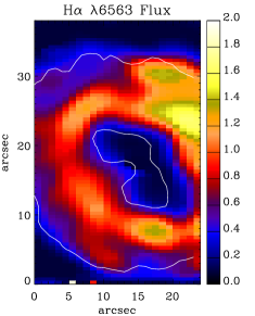
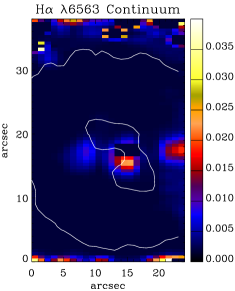
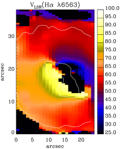
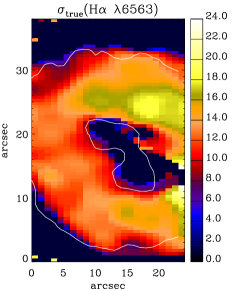
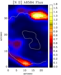
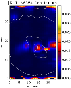
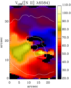
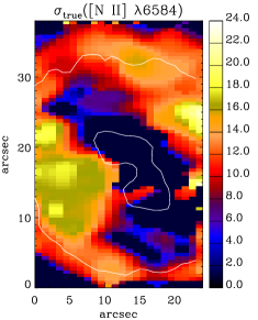
Figure 2: Maps of the PN Abell 48 in H$\alpha$ $\lambda$6563 Å (top) and $[$N ii$]$ $\lambda$6584 Å (bottom) from the IFU (${\rm PA}=0^{\circ}$) taken in 2010 April. From left to right: spatial distribution maps of flux intensity, continuum, LSR velocity and velocity dispersion. Flux unit is in $10^{-15}$ erg s^-1 cm^-2 spaxel^-1, continuum in $10^{-15}$ erg s^-1 cm^-2 Å^-1 spaxel^-1, and velocities in km s^-1. North is up and east is towards the left-hand side. The white contour lines show the distribution of the narrow-band emission of H$\alpha$ in arbitrary unit obtained from the SHS.

A complete list of observed emission lines and their flux intensities are given in Table 2 on a scale where H$\beta$ = 100. All fluxes were corrected for reddening using $I(\lambda)_{\rm corr}=F(\lambda)_{\rm obs}10^{c({\rm H}\beta)[1+f(\lambda)]}.$ The logarithmic $c({\rm H}\beta)$ value of the interstellar extinction for the case B recombination ($T_{\rm e}=10\,000$ K and $N_{\rm e}=1000$ cm^-3; Storey & Hummer, 1995) has been obtained from the H$\alpha$ and H$\beta$ Balmer fluxes. We used the Galactic extinction law $f(\lambda)$ of Howarth (1983) for $R_{V}=A(V)/E(B-V)=3.1$, and normalized such that $f({\rm H}\beta)=0$. We obtained an extinction of $c({\rm H}\beta)=3.1$ for the total fluxes (see Table 2). Our derived nebular extinction is in excellent agreement with the value derived by Todt et al. (2013) from the stellar spectral energy (SED). The same method was applied to create $c({\rm H}\beta)$ maps using the flux ratio H$\alpha$/H$\beta$, as shown in Fig. 1(b). Assuming that the foreground interstellar extinction is uniformly distributed over the nebula, an inhomogeneous extinction map may be related to some internal dust contributions. As seen, the extinction map of Abell 48 depicts that the shell is brighter than other regions, and it may contain the asymptotic giant branch (AGB) dust remnants.

3 Kinematics

Fig. 2 shows the spatial distribution maps of the flux intensity, continuum, radial velocity and velocity dispersion of H$\alpha$ $\lambda$6563 and $[$N ii$]$ $\lambda$6584 for Abell 48. The white contour lines in the figures depict the distribution of the emission of H$\alpha$ obtained from the SHS (Parker et al., 2005), which can aid us in distinguishing the nebular borders from the outside or the inside. The observed velocity $v_{\rm obs}$ was transferred to the local standard of rest (LSR) radial velocity $v_{\rm LSR}$ by correcting for the radial velocities induced by the motions of the Earth and Sun at the time of our observation. The transformation from the measured velocity dispersion $\sigma_{\rm obs}$ to the true line-of-sight velocity dispersion $\sigma_{\rm true}$ was done by $\sigma_{\rm true}=\sqrt{\sigma^{2}_{\rm obs}-\sigma^{2}_{\rm ins}-\sigma^{2}_{\rm th}}$, i.e. correcting for the instrumental width (typically $\sigma_{\rm ins}\approx 42$ km/s for $R\sim 3000$ and $\sigma_{\rm ins}\approx 18$ km/s for $R\sim 7000$) and the thermal broadening ($\sigma_{\rm th}^{2}=8.3\,T_{\rm e}[{\rm kK}]/Z$, where $Z$ is the atomic weight of the atom or ion).

(a) Morpho-kinematic mesh model

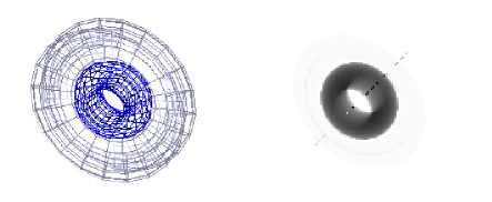
(b) Model results

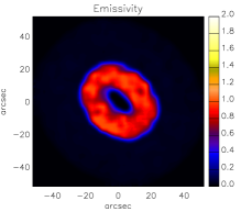
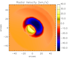
Figure 3: (a) The shape mesh model before rendering at the best-fitting inclination and corresponding rendered model. (b) The normalized synthetic intensity map and the radial velocity map at the inclination of $-35{}^{\circ}$ and the position angle of $135{}^{\circ}$, derived from the model ($v_{\rm sys}=0$), which can be compared directly with Fig. 2.

We have used the three-dimensional morpho-kinematic modelling program shape (version 4.5) to study the kinematic structure. The program described in detail by Steffen & López (2006) and Steffen et al. (2011), uses interactively moulded geometrical polygon meshes to generate the 3D structure of objects. The modelling procedure consists of defining the geometry, emissivity distribution and velocity law as a function of position. The program produces several outputs that can be directly compared with long slit or IFU observations, namely the position–velocity (P–V) diagram, the 2-D line-of-sight velocity map on the sky and the projected 3-D emissivity on the plane of the sky. The 2-D line-of-sight velocity map on the sky can be used to interpret the IFU velocity maps. For best comparison with the IFU maps, the inclination ($i$), the position angle ‘PA’ in the plane of the sky, and the model parameters are modified in an iterative process until the qualitatively fitting 3D emission and velocity information are produced. We adopted a model, and then modified the geometry and inclination to conform to the observed H$\alpha$ and [N ii] intensity and radial velocity maps. For this paper, the three-dimensional structure has then been transferred to a regular cell grid, together with the physical emission properties, including the velocity that, in our case, has been defined as radially outwards from the nebular centre with a linear function of magnitude, commonly known as a Hubble-type flow (see e.g. Steffen et al., 2009).

The morpho-kinematic model of Abell 48 is shown in Fig. 3(a), which consists of a modified torus, the nebular shell, surrounded by a modified hollow cylinder and the faint outer halo. The shell has an inner radius of $10\hbox{${}^{\prime\prime}$}$ and an outer radius of $23\hbox{${}^{\prime\prime}$}$ and a height of $23\hbox{${}^{\prime\prime}$}$. We found an expansion velocity of $v_{\rm exp}=35\pm 5$ km s^-1 and a LSR systemic velocity of $v_{\rm sys}=65\pm 5$ km s^-1. Our value of the LSR systemic velocity is in good agreement with the heliocentric systemic velocity of $v_{\rm hel}=50.4\pm 4.2$ km s^-1 found by Todt et al. (2013). Following Dopita et al. (1996), we estimated the nebula’s age around 1.5 of the dynamical age, so the star left the top of the AGB around $8880$ years ago.

Fig. 3 shows the orientation of Abell 48 on to the plane of the sky. The nebula has an inclination of $i=-35^{\circ}$ between the line of sight and the nebular symmetry axis. The symmetry axis has a position angle of ${\rm PA}=135^{\circ}$ projected on to the plane of the sky, measured from the north towards the east in the equatorial coordinate system (ECS). The PA in the ECS can be transferred into the Galactic position angle (GPA) in the Galactic coordinate system (GCS), measured from the north Galactic pole (NGP; ${\rm GPA}=0^{\circ}$) towards the Galactic east (${\rm GPA}=90^{\circ}$). Note that ${\rm GPA}=90^{\circ}$ describes an alignment with the Galactic plane, while ${\rm GPA}=0^{\circ}$ is perpendicular to the Galactic plane. As seen in Table 3, Abell 48 has a GPA of $197\aas@@fstack{\circ}8$, meaning that the symmetry axis is approximately perpendicular to the Galactic plane.

Based on the systemic velocity, Abell 48 must be located at less than 2 kpc, since higher distances result in very high peculiar velocities ($v_{\rm pec}>189$ km s^-1; $v_{\rm pec}=170$ km s^-1 found in few PNe in the Galactic halo by Maciel & Dutra, 1992). However, it cannot be less than 1.5 kpc due to the large interstellar extinction. Using the infrared dust maps of Schlegel et al. (1998), we found a mean reddening value of $E(B-V)=11.39\pm 0.64$ for an aperture of $10\hbox{${}^{\prime}$}$ in diameter in the Galactic latitudes and longitude of $(l,b)=(29.0,0.4)$, which is within a line-of-sight depth of $\lesssim 20$ kpc of the Galaxy. Therefore, Abell 48 with $E(B-V)\simeq 2.14$ must have a distance of less than $3.3$ kpc. Considering the fact that the Galactic bulge absorbs photons overall 1.9 times more than the Galactic disc (Driver et al., 2007), the distance of Abell 48 should be around 2 kpc, as it is located at the dusty Galactic disc.

Table 3: Kinematic results obtained for Abell 48 based on the morpho-kinematic model matched to the observed 2-D radial velocity map.

Parameter	Value
$r_{\rm out}$ (arcsec)	$23\pm 4$
$\delta r$ (arcsec)	$13\pm 2$
$h$ (arcsec)	$23\pm 4$
$i$	$-35^{\circ}\pm 2^{\circ}$
PA	$135^{\circ}\pm 2^{\circ}$
GPA	$197^{\circ}48\hbox{${}^{\prime}$}\pm 2^{\circ}$
$v_{\rm sys}$(km/s)	$65\pm 5$
$v_{\rm exp}$(km/s)	$35\pm 5$

4 Nebular empirical analysis

4.1 Plasma diagnostics

The derived electron temperatures ($T_{\rm e}$) and densities ($N_{\rm e}$) are listed in Table 5, together with the ionization potential required to create the emitting ions. We obtained $T_{\rm e}$ and $N_{\rm e}$ from temperature-sensitive and density-sensitive emission lines by solving the equilibrium equations of level populations for a multilevel atomic model using equib code (Howarth & Adams, 1981). The atomic data sets used for our plasma diagnostics from collisionally excited lines (CELs), as well as for abundances derived from CELs, are given in Table 4. The diagnostics procedure to determine temperatures and densities from CELs is as follows: we assume a representative initial electron temperature of 10 000 K in order to derive $N_{\rm e}$ from $[$S ii$]$ line ratio; then $T_{\rm e}$ is derived from $[$N ii$]$ line ratio in conjunction with the mean density derived from the previous step. The calculations are iterated to give self-consistent results for $N_{\rm e}$ and $T_{\rm e}$. The correct choice of electron density and temperature is important for the abundance determination.

We see that the PN Abell 48 has a mean temperature of $T_{\rm e}([$N ii$])=6980\pm 930$ K, and a mean electron density of $N_{\rm e}([$S ii$])=750\pm 200$ cm^-3, which are in reasonable agreement with $T_{\rm e}([$N ii$])=7\,200\pm 750$ K and $N_{\rm e}([$S ii$])=1000\pm 130$ cm^-3 found by Todt et al. (2013). The uncertainty on $T_{\rm e}([$N ii$])$ is order of $40$ percent or more, due to the weak flux intensity of [N ii] $\lambda$5755, the recombination contribution, and high interstellar extinction. Therefore, we adopted the mean electron temperature from our photoionization model for our CEL abundance analysis.

Table 4: References for atomic data.

Ion	Transition probabilities	Collision strengths
N+	Bell et al. (1995)	Stafford et al. (1994)
O+	Zeippen (1987)	Pradhan et al. (2006)
O2+	Storey & Zeippen (2000)	Lennon & Burke (1994)
Ne2+	Landi & Bhatia (2005)	McLaughlin & Bell (2000)
S+	Mendoza & Zeippen (1982)	Ramsbottom et al. (1996)
S2+	Mendoza & Zeippen (1982)	Tayal & Gupta (1999)
	Huang (1985)
Ar2+	Biémont & Hansen (1986)	Galavis et al. (1995)
Ion	Recombination coefficient	Case
H+	Storey & Hummer (1995)	B
He+	Porter et al. (2013)	B
C2+	Davey et al. (2000)	B

Table 5 also lists the derived He i temperatures, which are lower than the CEL temperatures, known as the ORL-CEL temperature discrepancy problem in PNe (see e.g. Liu et al., 2000, 2004b). To determine the electron temperature from the He i $\lambda\lambda$5876, 6678 and 7281 lines, we used the emissivities of He I lines by Smits (1996), which also include the temperature range of $T_{\rm e}<5000$ K. We derived electron temperatures of $T_{\rm e}({\rm He~{}I})=5110$ K and $T_{\rm e}({\rm He~{}I})=4360$ K from the flux ratio He i $\lambda\lambda$7281/5876 and $\lambda\lambda$7281/6678, respectively. Similarly, we got $T_{\rm e}({\rm He~{}I})=6960$ K for He i $\lambda\lambda$7281/5876 and $T_{\rm e}({\rm He~{}I})=7510$ K for $\lambda\lambda$7281/6678 from the measured nebular spectrum by Todt et al. (2013).

Table 5: Diagnostics for the electron temperature, $T_{\rm e}$ and the electron density, $N_{\rm e}$. References: D13 – this work; T13 – Todt et al. (2013).

Ion	Diagnostic	I.P.(eV)	$T_{\rm e}({\rm K})$	Ref.
$[$N ii$]$	$\frac{\lambda 6548+\lambda 6584}{\lambda 5755}$	14.53	$6980\pm 930$	D13
			$7200\pm 750$	T13
$[$O iii$]$	$\frac{\lambda 4959+\lambda 5007}{\lambda 4363}$	35.12	$11870\pm 1640$	T13
He i	$\frac{\lambda 7281}{\lambda 5876}$	24.59	$5110\pm 2320$	D13
			$6960\pm 450$	T13
He i	$\frac{\lambda 7281}{\lambda 6678}$	24.59	$4360\pm 1820$	D13
			$7510\pm 4800$	T13
			$N_{\rm e}({\rm cm}^{-3})$
$[$S ii$]$	$\frac{\lambda 6717}{\lambda 6731}$	10.36	$750\pm 200$	D13
			$1000\pm 130$	T13

4.2 Ionic and total abundances from ORLs

Using the effective recombination coefficients (given in Table 4), we determine ionic abundances, Xⁱ⁺/H⁺, from the measured intensities of optical recombination lines (ORLs) as follows:

$$\frac{N({\rm X}^{i+})}{N({\rm H}^{+})}=\frac{I({\lambda})}{I({{\rm H}\beta})}\frac{\lambda({\rm{\AA}})}{4861}\frac{\alpha_{\rm eff}({\rm H}\beta)}{\alpha_{\rm eff}(\lambda)},$$ (1)

where $I({\lambda})$ is the intrinsic line flux of the emission line $\lambda$ emitted by ion ${\rm X}^{i+}$, $I({{\rm H}\beta})$ is the intrinsic line flux of H$\beta$, $\alpha_{\rm eff}({\rm H}\beta)$ the effective recombination coefficient of H$\beta$, and $\alpha_{\rm eff}(\lambda)$ the effective recombination coefficient for the emission line $\lambda$.

Abundances of helium and carbon from ORLs are given in Table 6. We derived the ionic and total helium abundances from He i $\lambda$4471, $\lambda$5876 and $\lambda$6678 lines. We assumed the Case B recombination for the He i lines (Porter et al., 2012, 2013). We adopted an electron temperature of $T_{\rm e}=5\,000$ K from He i lines, and an electron density of $N_{\rm e}=1000$ cm^-3. We averaged the He⁺/H⁺ ionic abundances from the He i $\lambda$4471, $\lambda$5876 and $\lambda$6678 lines with weights of 1:3:1, roughly the intrinsic intensity ratios of these three lines. The total He/H abundance ratio is obtained by simply taking the sum of He⁺/H⁺ and He²⁺/H⁺. However, He²⁺/H⁺ is equal to zero, since He ii $\lambda$4686 is not present. The C²⁺ ionic abundance is obtained from C ii $\lambda$6462 and $\lambda$7236 lines.

Table 6: Empirical ionic abundances derived from ORLs.

Ion	$\lambda$(Å)	Mult	Value a
He+	4471.50	V14	0.141
	5876.66	V11	0.121
	6678.16	V46	0.115
	Mean		0.124
He2+	4685.68	3.4	0.0
He/H			0.124
C2+	6461.95	V17.40	3.068($-3$)
	7236.42	V3	1.254($-3$)
	Mean		2.161($-3$)

• Assuming $T_{\rm e}=5\,000$ K and $N_{\rm e}=1000$ ${\rm cm}^{-3}$.

4.3 Ionic and total abundances from CELs

We determined abundances for ionic species of N, O, Ne, S and Ar from CELs. To deduce ionic abundances, we solve the statistical equilibrium equations for each ion using equib code, giving level population and line sensitivities for specified $N_{\rm e}=1000$ cm^-3 and $T_{\rm e}=10\,000$ K adopted according to our photoionization modelling. Once the equations for the population numbers are solved, the ionic abundances, Xⁱ⁺/H⁺, can be derived from the observed line intensities of CELs as follows:

$$\frac{N({\rm X}^{i+})}{N({\rm H}^{+})}=\frac{I(\lambda_{ij})}{I({{\rm H}\beta})}\frac{\lambda_{ij}({\rm{\AA}})}{4861}\frac{\alpha_{\rm eff}({{\rm H}\beta})}{A_{ij}}\frac{N_{\rm e}}{n_{i}},$$ (2)

where $I(\lambda_{ij})$ is the dereddened flux of the emission line $\lambda_{ij}$ emitted by ion ${\rm X}^{i+}$ following the transition from the upper level $i$ to the lower level $j$, $I({{\rm H}\beta})$ the dereddened flux of H$\beta$, $\alpha_{\rm eff}({{\rm H}\beta})$ the effective recombination coefficient of H$\beta$, $A_{ij}$ the Einstein spontaneous transition probability of the transition, $n_{i}$ the fractional population of the upper level $i$, and $N_{\rm e}$ is the electron density.

Total elemental and ionic abundances of nitrogen, oxygen, neon, sulphur and argon from CELs are presented in Table 7. Total elemental abundances are derived from ionic abundances using the ionization correction factors ($icf$) formulas given by Kingsburgh & Barlow (1994). The total O/H abundance ratio is obtained by simply taking the sum of the O⁺/H⁺ derived from [O ii] $\lambda\lambda$3726,3729 doublet, and the O²⁺/H⁺ derived from [O iii] $\lambda\lambda$4959,5007 doublet, since He ii $\lambda$4686 is not present, so O³⁺/H⁺ is negligible. The total N/H abundance ratio was calculated from the N⁺/H⁺ ratio derived from the [N ii] $\lambda\lambda$6548,6584 doublet, correcting for the unseen N²⁺/H⁺ using,

$$\footnotesize\frac{{\rm N}}{{\rm H}}=\left(\frac{{\rm N}^{+}}{{\rm H}^{+}}\right)\left(\frac{{\rm O}}{{\rm O}^{+}}\right).$$ (3)

The Ne²⁺/H⁺ is derived from [Ne iii] $\lambda$3869 line. Similarly, the unseen Ne⁺/H⁺ is corrected for, using

$$\frac{{\rm Ne}}{{\rm H}}=\left(\frac{{\rm Ne}^{2+}}{{\rm H}^{+}}\right)\left(\frac{{\rm O}}{{\rm O}^{2+}}\right).$$ (4)

For sulphur, we have S⁺/H⁺ from the [S ii] $\lambda\lambda$6716,6731 doublet and S²⁺/H⁺ from the [S iii] $\lambda$9069 line. The total sulphur abundance is corrected for the unseen stages of ionization using

$$\footnotesize\frac{{\rm S}}{{\rm H}}=\left(\frac{{\rm S}^{+}}{{\rm H}^{+}}+\frac{{\rm S}^{2+}}{{\rm H}^{+}}\right)\left[1-\left(1-\frac{{\rm O}^{+}}{{\rm O}}\right)^{3}\right]^{-1/3}.$$ (5)

The [Ar iii] 7136 line is only detected, so we have only Ar²⁺/H⁺. The total argon abundance is obtained by assuming Ar⁺/Ar = N⁺/N:

$$\footnotesize\frac{{\rm Ar}}{{\rm H}}=\left(\frac{{\rm Ar}^{2+}}{{\rm H}^{+}}\right)\left(1-\frac{{\rm N}^{+}}{{\rm N}}\right)^{-1}.$$ (6)

As it does not include the unseen Ar³⁺, so the derived elemental argon may be underestimated.

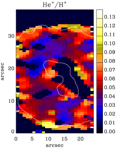
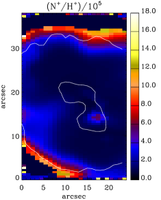
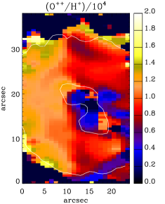
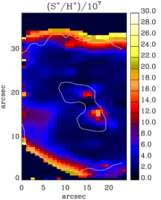
Figure 4: Ionic abundance maps of Abell 48. From left to right: spatial distribution maps of singly ionized Helium abundance ratio He⁺/H⁺ from He i ORLs (4472, 5877, 6678); ionic nitrogen abundance ratio N⁺/H⁺ ($\times 10^{-5}$) from $[$N ii$]$ CELs (5755, 6548, 6584); ionic oxygen abundance ratio O²⁺/H⁺ ($\times 10^{-4}$) from $[$O iii$]$ CELs (4959, 5007); and ionic sulphur abundance ratio S⁺/H⁺ ($\times 10^{-7}$) from $[$S ii$]$ CELs (6716, 6731). North is up and east is towards the left-hand side. The white contour lines show the distribution of the narrow-band emission of H$\alpha$ in arbitrary unit obtained from the SHS.

Fig. 4 shows the spatial distribution of ionic abundance ratio He⁺/H⁺, N⁺/H⁺, O²⁺/H⁺ and S⁺/H⁺ derived for given $T_{\rm e}=10000$ K and $N_{\rm e}=1000$ cm^-3. We notice that both O²⁺/H⁺ and He⁺/H⁺ are very high over the shell, whereas N⁺/H⁺ and S⁺/H⁺ are seen at the edges of the shell. It shows obvious results of the ionization sequence from the highly inner ionized zones to the outer low ionized regions.

Table 7: Empirical ionic abundances derived from CELs.

Ion	$\lambda$(Å)	Mult	Value a
N+	6548.10	F1	1.356($-5$)
	6583.50	F1	1.486($-5$)
	Mean		1.421($-5$)
	$icf$(N)		3.026
N/H			4.299($-5$)
O+	3727.43	F1	5.251($-5$)
O2+	4958.91	F1	1.024($-4$)
	5006.84	F1	1.104($-4$)
	Average		1.064($-4$)
	$icf$(O)		1.0
O/H			1.589($-4$)
Ne2+	3868.75	F1	4.256($-5$)
	$icf$(Ne)		1.494
Ne/H			6.358($-5$)
S+	6716.44	F2	4.058($-7$)
	6730.82	F2	3.896($-7$)
	Average		3.977($-7$)
S2+	9068.60	F1	5.579($-6$)
	$icf$(S)		1.126
S/H			6.732($-6$)
Ar2+	7135.80	F1	9.874($-7$)
	$icf$(Ar)		1.494
Ar/H			1.475($-6$)

• Assuming $T_{\rm e}=10\,000$ K and $N_{\rm e}=1000$ ${\rm cm}^{-3}$.

5 Photoionization modelling

The 3-D photoionization code mocassin (version 2.02.67; Ercolano et al., 2003b, 2005, 2008) was used to study the best-fitting model for Abell 48. The code has been used to model a number of PNe, for example NGC 3918 (Ercolano et al., 2003a), NGC 7009 (Gonçalves et al., 2006), NGC 6302 (Wright et al., 2011), and SuWt 2 (Danehkar et al., 2013). The modelling procedure consists of defining the density distribution and elemental abundances of the nebula, as well as assigning the ionizing spectrum of the CS. This code uses a Monte Carlo method to solve self-consistently the 3-D radiative transfer of the stellar radiation field in a gaseous nebula with the defined density distribution and chemical abundances. It produces the emission-line spectrum, the thermal structure and the ionization structure of the nebula. It allows us to determine the stellar characteristics and the nebula parameters. The atomic data sets used for the calculation are energy levels, collision strengths and transition probabilities from the CHIANTI data base (version 5.2; Landi et al., 2006), hydrogen and helium free–bound coefficients of Ercolano & Storey (2006), and opacities from Verner et al. (1993) and Verner & Yakovlev (1995).

The best-fitting model was obtained through an iterative process, involving the comparison of the predicted H$\beta$ luminosity $L_{{\rm H}\beta}$(erg s^-1), the flux intensities of some important lines, relative to H$\beta$ (such as $[$O iii$]$ $\lambda$5007 and $[$N ii$]$ $\lambda$6584), with those measured from the observations. The free parameters included distance and nebular parameters. We initially used the stellar luminosity ($L_{\star}=6000$ L_⨀) and effective temperature ($T_{\rm eff}=70$kK) found by Todt et al. (2013). However, we slightly adjusted the stellar luminosity to match the observed line flux of $[$O iii$]$ emission line. Moreover, we adopted the nebular density and abundances derived from empirical analysis in Section 4, but they have been gradually adjusted until the observed nebular emission-line spectrum was reproduced by the model. The best-fitting $L_{{\rm H}\beta}$ depends upon the distance and nebula density. The plasma diagnostics yields $N_{\rm e}=750$–1000 cm^-3, which can be an indicator of the density range. Based on the kinematic analysis, the distance must be less than 2 kpc, but more than 1.5 kpc due to the large interstellar extinction. We matched the predicted H$\beta$ luminosity $L({\rm H}\beta)$ with the value derived from the observation by adjusting the distance and nebular density. Then, we adjusted abundances to get the best emission-line spectrum.

5.1 The ionizing spectrum

The hydrogen-deficient synthetic spectra of Abell 48 was modelled using stellar model atmospheres produced by the Potsdam Wolf–Rayet (PoWR) models for expanding atmospheres (Gräfener et al., 2002; Hamann & Gräfener, 2004). It solves the non-local thermodynamic equilibrium (non-LTE) radiative transfer equation in the comoving frame, iteratively with the equations of statistical equilibrium and radiative equilibrium, for an expanding atmosphere under the assumptions of spherical symmetry, stationarity and homogeneity. The result of our model atmosphere is shown in Fig. 5. The model atmosphere calculated with the PoWR code is for the stellar surface abundances H:He:C:N:O = 10:85:0.3:5:0.6 by mass, the stellar temperature $T_{\rm eff}$ = 70 kK, the transformed radius $R_{\rm t}=0.54$ R_⨀ and the wind terminal velocity $v_{\infty}=1000$ km s^-1. The best photoionization model was obtained with an effective temperature of 70 kK (the same as PoWR model used by Todt et al., 2013) and a stellar luminosity of $L_{\rm\star}/$L_⨀= 5500, which is close to $L_{\star}/$L_⨀= 6000 adopted by Todt et al. (2013). This stellar luminosity was found to be consistent with the observed H$\beta$ luminosity and the flux ratio of $[$O iii$]$/H$\beta$. A stellar luminosity higher than 5500 L_⨀ produces inconsistent results for the nebular photoionization modelling. The emission-line spectrum produced by our adopted stellar parameters was found to be consistent with the observations.

Table 8: Input parameters for the mocassin photoionization model.

Stellar and Nebular			Nebular Abundances
Parameters			Model	Obs.
$T_{\rm eff}$ (kK)	70	He/H	0.120	0.124
$L_{\rm\star}$ (L⨀)	5500	C/H $\times 10^{3}$	3.00	–
$N_{\rm H}$ (cm-3)	800-1200	N/H $\times 10^{5}$	6.50	4.30
$D$ (kpc)	1.9	O/H $\times 10^{4}$	1.40	1.59
$r_{\rm out}$ (arcsec)	23	Ne/H $\times 10^{5}$	6.00	6.36
$\delta r$ (arcsec)	13	S/H $\times 10^{6}$	6.00	6.73
$h$ (arcsec)	23	Ar/H $\times 10^{6}$	1.20	1.48

5.2 The density distribution

We initially used a three-dimensional uniform density distribution, which was developed from our kinematic analysis. However, the interacting stellar winds (ISW) model developed by Kwok et al. (1978) demonstrated that a slow dense superwind from the AGB phase is swept up by a fast tenuous wind during the PN phase, creating a compressed dense shell, which is similar to what we see in Fig. 6. Additionally, Kahn & West (1985) extended the ISW model to describe a highly elliptical mass distribution. This extension later became known as the generalized interacting stellar winds theory. There are a number of hydrodynamic simulations, which showed the applications of the ISW theory for bipolar PNe (see e.g. Mellema, 1996, 1997). As shown in Fig. 6, we adopted a density structure with a toroidal wind mass-loss geometry, similar to the ISW model. In our model, we defined a density distribution in the cylindrical coordinate system, which has the form $N_{\rm H}(r)=N_{0}[1+(r/r_{\rm in})^{-\alpha}],$ where $r$ is the radial distance from the centre, $\alpha$ the radial density dependence, $N_{0}$ the characteristic density, $r_{\rm in}=r_{\rm out}-\delta r$ the inner radius, $r_{\rm out}$ the outer radius and $\delta r$ the thickness.

The density distribution is usually a complicated input parameter to constrain. However, the values found from our plasma diagnostics ($N_{\rm e}=750$–1000 cm^-3) allowed us to constrain our density model. The outer radius and the height of the cylinder are equal to $r_{\rm out}=23\hbox{${}^{\prime\prime}$}$ and the thickness is $\delta r=13\hbox{${}^{\prime\prime}$}$. The density model and distance (size) were adjusted in order to reproduce $I$(H$\beta)=1.355\times 10^{-10}$ erg s^-1 cm^-2, dereddened using c(H$\beta$) = 3.1 (see Section 2). We tested distances, with values ranging from 1.5 to 2.0 kpc. We finally adopted the characteristic density of $N_{0}=600$ cm^-3 and the radial density dependence of $\alpha=1$. The value of 1.90 kpc found here, was chosen, because of the best predicted H$\beta$ luminosity, and it is in excellent agreement with the distance constrained by the synthetic spectral energy distribution (SED) from the PoWR models. Once the density distribution and distance were identified, the variation of the nebular ionic abundances were explored.

Table 9: Dereddened observed and predicted emission-line fluxes for Abell 48. References: D13 – this work; T13 – Todt et al. (2013). Uncertain and very uncertain values are followed by ‘:’ and ‘::’, respectively. The symbol ‘*’ denotes blended emission lines.

Line	Observed		Predicted
	D13	T13
$I$(H$\beta$)/10${}^{-10}\,\frac{\rm erg}{\rm cm^{2}s}$	1.355	–	1.371
H$\beta$ 4861	100.00	100.00	100.00
H$\alpha$ 6563	286.00	290.60	285.32
H$\gamma$ 4340	54.28:	45.10	46.88
H$\delta$ 4102	–	–	25.94
He i 4472	7.42:	–	6.34
He i 5876	18.97	20.60	17.48
He i 6678	5.07	4.80	4.91
He i 7281	0.58::	0.70	0.97
He ii 4686	–	–	0.00
C ii 6462	0.38	–	0.27
C ii 7236	1.63	–	1.90
$[$N ii$]$ 5755	0.43::	0.40	1.20
$[$N ii$]$ 6548	26.09	28.20	26.60
$[$N ii$]$ 6584	87.28	77.00	81.25
$[$O ii$]$ 3726	128.96:	–	59.96
$[$O ii$]$ 3729	*	–	43.54
$[$O ii$]$ 7320	–	0.70	2.16
$[$O ii$]$ 7330	–	0.60	1.76
$[$O iii$]$ 4363	–	3.40	2.30
$[$O iii$]$ 4959	99.28	100.50	111.82
$[$O iii$]$ 5007	319.35	316.50	333.66
$[$Ne iii$]$ 3869	38.96	–	39.60
$[$Ne iii$]$ 3967	–	–	11.93
$[$S ii$]$ 4069	–	–	1.52
$[$S ii$]$ 4076	–	–	0.52
$[$S ii$]$ 6717	7.44	5.70	10.30
$[$S ii$]$ 6731	7.99	6.80	10.57
$[$S iii$]$ 6312	0.60::	–	2.22
$[$S iii$]$ 9069	19.08	–	16.37
$[$Ar iii$]$ 7136	10.88	10.20	12.75
$[$Ar iii$]$ 7751	4.00::	–	3.05
$[$Ar iv$]$ 4712	–	–	0.61
$[$Ar iv$]$ 4741	–	–	0.51

5.3 The nebular elemental abundances

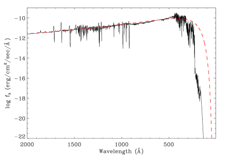
Figure 5: Non-LTE model atmosphere flux (solid line) calculated with the PoWR models for the surface abundances H:He:C:N:O = 10:85:0.3:5:0.6 by mass and the stellar temperature $T_{\rm eff}$ = 70 kK, compared with a blackbody (dashed line) at the same temperature.

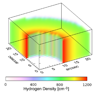
Figure 6: The density distribution based on the ISW models adopted for photoionization modelling of Abell 48. The cylinder has outer radius of $23\hbox{${}^{\prime\prime}$}$ and thickness of $13\hbox{${}^{\prime\prime}$}$. Axis units are arcsec, where 1 arcsec is equal to $9.30\times 10^{-3}$ pc based on the distance determined by our photoionization model.

Table 8 lists the nebular elemental abundances (with respect to H) used for the photoionization model. We used a homogeneous abundance distribution, since we do not have any direct observational evidence for the presence of chemical inhomogeneities. Initially, we used the abundances from empirical analysis as initial values for our modelling (see Section 4). They were successively modified to fit the optical emission-line spectrum through an iterative process. We obtain a C/O ratio of 21 for Abell 48, indicating that it is predominantly C-rich. Furthermore, we find a helium abundance of 0.12. This can be an indicator of a large amount of mixing processing in the He-rich layers during the He-shell flash leading to an increase carbon abundance. The nebulae around H-deficient CSs typically have larger carbon abundances than those with H-rich CSs (see review by De Marco & Barlow, 2001). The ${\rm O}/{\rm H}$ we derive for Abell 48 is lower than the solar value (${\rm O}/{\rm H}=4.57\times 10^{-4}$; Asplund et al., 2009). This may be due to that the progenitor has a sub-solar metallicity. The enrichment of carbon can be produced in a very intense mixing process in the He-shell flash (Herwig et al., 1997). Other elements seem to be also decreased compared to the solar values, such as sulphur and argon. Sulphur could be depleted on to dust grains (Sofia et al., 1994), but argon cannot have any strong depletion by dust formation (Sofia & Jenkins, 1998). We notice that the N/H ratio is about the solar value given by Asplund et al. (2009), but it can be produced by secondary conversion of initial carbon if we assume a sub-solar metallicity progenitor. The combined (C+N+O)/H ratio is by a factor of 3.9 larger than the solar value, which can be produced by multiple dredge-up episodes occurring in the AGB phase.

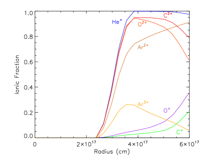
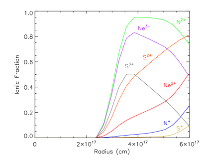
Figure 7: Top: electron density and temperature as a function of radius along the equatorial direction. Bottom: ionic stratification of the nebula. Ionization fractions are shown for helium, carbon, oxygen, argon (left-hand panel), nitrogen, neon and sulphur (right-hand panel).

Table 10: Fractional ionic abundances for Abell 48 obtained from the photoionization model.

	Ion
Element	i	ii	iii	iv	v	vi	vii
H	3.84($-2$)	9.62($-1$)
He	3.37($-2$)	9.66($-1$)	1.95($-6$)
C	5.43($-4$)	1.73($-1$)	8.18($-1$)	8.93($-3$)	1.64($-15$)	1.00($-20$)	1.00($-20$)
N	1.75($-2$)	1.94($-1$)	7.79($-1$)	8.98($-3$)	2.72($-15$)	1.00($-20$)	1.00($-20$)
O	4.32($-2$)	2.60($-1$)	6.97($-1$)	1.18($-7$)	3.09($-20$)	1.00($-20$)	1.00($-20$)
Ne	9.94($-3$)	3.88($-1$)	6.03($-1$)	1.12($-13$)	1.00($-20$)	1.00($-20$)	1.00($-20$)
S	6.56($-5$)	8.67($-2$)	6.99($-1$)	2.12($-1$)	2.42($-3$)	1.66($-15$)	1.00($-20$)
Ar	2.81($-3$)	3.74($-2$)	8.43($-1$)	1.17($-1$)	1.02($-13$)	1.00($-20$)	1.00($-20$)

6 Model results

6.1 Comparison of the emission-line fluxes

Table 9 compares the flux intensities predicted by the best-fitting model with those from the observations. Columns 2 and 3 present the dereddened fluxes of our observations and those from Todt et al. (2013). The predicted emission-line fluxes are given in Column 4, relative to the intrinsic dereddened H$\beta$ flux, on a scale where $I($H$\beta)$ = 100. The most emission-line fluxes presented are in reasonable agreement with the observations. However, we notice that the [O ii] $\lambda$7319 and $\lambda$7330 doublets are overestimated by a factor of 3, which can be due to the recombination contribution. Our photoionization code incorporates the recombination term to the statistical equilibrium equations. However, the recombination contribution are less than 30 per cent for the values of $T_{\rm e}$ and $N_{\rm e}$ found from the plasma diagnostics. Therefore, the discrepancy between our model and observed intensities of these lines can be due to inhomogeneous condensations such as clumps and/or colder small-scale structures embedded in the global structure. It can also be due to the measurement errors of these weak lines. The [O ii] $\lambda\lambda$3726,3729 doublet predicted by the model is around 25 per cent lower, which can be explained by either the recombination contribution or the flux calibration error. There is a notable discrepancy in the predicted [N ii] $\lambda$5755 auroral line, being higher by a factor of $\sim 3$. It can be due to the errors in the flux measurement of the [N ii] $\lambda$5755 line. The predicted [Ar iii] $\lambda$7751 line is also 30 per cent lower, while [Ar iii] $\lambda$7136 is about 20 per cent higher. The [Ar iii] $\lambda$7751 line usually is blended with the telluric line, so the observed intensity of these line can be overestimated. It is the same for [S iii] $\lambda$9069, which is typically affected by the atmospheric absorption band.

Table 11: Integrated ionic abundance ratios for He, C, N, O, Ne, S and Ar, derived from model ionic fractions and compared to those from the empirical analysis.

Ionic ratio	Observed	Model
He+/H+	0.124	0.116
C2+/H+	2.16($-3$)	2.45($-3$)
N+/H+	1.42($-5$)	1.26($-5$)
O+/H+	5.25($-5$)	3.63($-5$)
O2+/H+	1.06($-4$)	9.76($-5$)
Ne2+/H+	4.26($-5$)	3.62($-5$)
S+/H+	3.98($-7$)	5.20($-7$)
S2+/H+	5.58($-6$)	4.19($-6$)
Ar2+/H+	9.87($-7$)	1.01($-6$)

6.2 Ionization and thermal structure

The volume-averaged fractional ionic abundances are listed in Table 10. We note that hydrogen and helium are singly-ionized. We see that the O⁺/O ratio is higher than the N⁺/N ratio by a factor of 1.34, which is dissimilar to what is generally assumed in the $icf$ method. However, the O²⁺/O ratio is nearly a factor of 1.16 larger than the Ne²⁺/Ne ratio, in agreement with the general assumption for $icf$(Ne). We see that only 19 per cent of the total nitrogen in the nebula is in the form of N⁺. However, the total oxygen largely exists as O²⁺ with 70 per cent and then O⁺ with 26 per cent.

The elemental abundances we used for the photoionization model returns ionic abundances listed in Table 11, are comparable to those from the empirical analysis derived in Section 4. The ionic abundances derived from the observations do not show major discrepancies in He⁺/H⁺, C²⁺/H⁺, N⁺/H⁺, O²⁺/H⁺, Ne²⁺/H⁺ and Ar²⁺/H⁺; differences remain below 18 per cent. However, the predicted and empirical values of O⁺/H⁺, S⁺/H⁺ and S²⁺/H⁺ have discrepancies of about 45, 31 and 33 per cent, respectively.

Fig. 7(bottom) shows plots of the ionization structure of helium, carbon, oxygen, argon (left-hand panel), nitrogen, neon and sulphur (right-hand panel) as a function of radius along the equatorial direction. As seen, ionization layers have a clear ionization sequence from the highly ionized inner parts to the outer regions. Helium is 97 percent singly-ionized over the shell, while oxygen is 26 percent singly ionized and 70 percent doubly ionized. Carbon and nitrogen are about $\sim 20$ percent singly ionized $\sim 80$ percent doubly ionized. The distribution of N⁺ is in full agreement with the IFU map, given in Fig 4. Comparison between the He⁺, O²⁺ and S⁺ ionic abundance maps obtained from our IFU observations and the ionic fractions predicted by our photoionization model also show excellent agreement.

Table 12: Mean electron temperatures (K) weighted by ionic species for the whole nebula obtained from the photoionization model.

	Ion
El.	i	ii	iii	iv	v	vi	vii
H	9044	10194
He	9027	10189	10248
C	9593	9741	10236	10212	10209	10150	10150
N	8598	9911	10243	10212	10209	10150	10150
O	9002	10107	10237	10241	10211	10150	10150
Ne	8672	10065	10229	10225	10150	10150	10150
S	9386	9388	10226	10208	10207	10205	10150
Ar	8294	9101	10193	10216	10205	10150	10150

Table 12 lists mean temperatures weighted by the ionic abundances. Both [N ii] and [O iii] doublets, as well as He i lines arise from the same ionization zones, so they should have roughly similar values. The ionic temperatures increasing towards higher ionization stages could also have some implications for the mean temperatures averaged over the entire nebula. However, there is a large discrepancy by a factor of 2 between our model and ORL empirical value of $T_{\rm e}$(He i$)$. This could be due to some temperature fluctuations in the nebula (Peimbert, 1967, 1971). The temperature fluctuations lead to overestimating the electron temperature deduced from CELs. This can lead to the discrepancies in abundances determined from CELs and ORLs (see e.g. Liu et al., 2000). Nevertheless, the temperature discrepancy can also be produced by bi-abundance models (Liu, 2003; Liu et al., 2004a), containing some cold hydrogen-deficient material, highly enriched in helium and heavy elements, embedded in the diffuse warm nebular gas of normal abundances. The existence and origin of such inclusions are still unknown. It is unclear whether there is any link between the assumed H-poor inclusions in PNe and the H-deficient CSs.

7 Conclusion

We have constructed a photoionization model for the nebula of Abell 48. This consists of a dense hollow cylinder, assuming homogeneous abundances. The three-dimensional density distribution was interpreted using the morpho-kinematic model determined from spatially resolved kinematic maps and the ISW model. Our aim was to construct a model that can reproduce the nebular emission-line spectra, temperatures and ionization structure determined from the observations. We have used the non-LTE model atmosphere from Todt et al. (2013) as the ionizing source. Using the empirical analysis methods, we have determined the temperatures and the elemental abundances from CELs and ORLs. We notice a discrepancy between temperatures estimated from $[$O iii$]$ CELs and those from the observed He i ORLs. In particular, the abundance ratios derived from empirical analysis could also be susceptible to inaccurate values of electron temperature and density. However, we see that the predicted ionic abundances are in decent agreement with those deduced from the empirical analysis. The emission-line fluxes obtained from the model were in fair agreement with the observations.

We notice large discrepancies between He i electron temperatures derived from the model and the empirical analysis. The existence of clumps and low-ionization structures could solve the problems (Liu et al., 2000). Temperature fluctuations have been also proposed to be responsible for the discrepancies in temperatures determined from CELs and ORLs (Peimbert, 1967, 1971). Previously, we also saw large ORL–CEL abundance discrepancies in other PNe with hydrogen-deficient CSs, for example Abell 30 (Ercolano et al., 2003a) and NGC 1501 (Ercolano et al., 2004). A fraction of H-deficient inclusions might produce those discrepancies, which could be ejected from the stellar surface during a very late thermal pulse (VLTP) phase or born-again event (Iben & Renzini, 1983). However, the VLTP event is expected to produce a carbon-rich stellar surface abundance (Herwig, 2001), whereas in the case of Abell 48 negligible carbon was found at the stellar surface (C/He = $3.5\times 10^{-3}$ by mass; Todt et al., 2013). The stellar evolution of Abell 48 still remains unclear and needs to be investigated further. But, its extreme helium-rich atmosphere (85 per cent by mass) is more likely connected to a merging process of two white dwarfs as evidenced for R Cor Bor stars of similar chemical surface composition by observations (Clayton et al., 2007; García-Hernández et al., 2009) and hydrodynamic simulations (Staff et al., 2012; Zhang & Jeffery, 2012; Menon et al., 2013).

We derived a nebula ionized mass of $\sim 0.8$ M_⨀. The high C/O ratio indicates that it is a predominantly C-rich nebula. The C/H ratio is largely over-abundant compared to the solar value of Asplund et al. (2009), while oxygen, sulphur and argon are under-abundant. Moreover, nitrogen and neon are roughly similar to the solar values. Assuming a sub-solar metallicity progenitor, a 3rd dredge-up must have enriched carbon and nitrogen in AGB-phase. However, extremely high carbon must be produced through mixing processing in the He-rich layers during the He-shell flash. The low N/O ratio implies that the progenitor star never went through the hot bottom burning phase, which occurs in AGB stars with initial masses more than 5M_⨀ (Karakas & Lattanzio, 2007; Karakas et al., 2009). Comparing the stellar parameters found by the model, $T_{\rm eff}$ = 70 kK and $L_{\rm\star}/$L_⨀= 5500, with VLTP evolutionary tracks from Blöcker (1995), we get a current mass of $\sim 0.62{\rm M}_{\bigodot}$, which originated from a progenitor star with an initial mass of $\sim 3{\rm M}_{\bigodot}$. However, the VLTP evolutionary tracks by Miller Bertolami & Althaus (2006) yield a current mass of $\sim 0.52{\rm M}_{\bigodot}$ and a progenitor mass of $\sim 1{\rm M}_{\bigodot}$, which is not consistent with the derived nebula ionized mass. Furthermore, time-scales for VLTP evolutionary track (Blöcker, 1995) imply that the CS has a post-AGB age of about $\sim$ 9 000 yr, in agreement with the nebula’s age determined from the kinematic analysis. We therefore conclude that Abell 48 originated from an $\sim 3$ M_⨀ progenitor, which is consistent with the nebula’s features.

References

- Abell (1955) Abell G. O., 1955, PASP, 67, 258
- Asplund et al. (2009) Asplund M., Grevesse N., Sauval A. J., Scott P., 2009, ARA&A, 47, 481
- Bell et al. (1995) Bell K. L., Hibbert A., Stafford R. P., 1995, Phys. Scr, 52, 240
- Biémont & Hansen (1986) Biémont E., Hansen J. E., 1986, Phys. Scr, 34, 116
- Blöcker (1995) Blöcker T., 1995, A&A, 299, 755
- Clayton et al. (2007) Clayton G. C., Geballe T. R., Herwig F., Fryer C., Asplund M., 2007, ApJ, 662, 1220
- Danehkar et al. (2013) Danehkar A., Parker Q. A., Ercolano B., 2013, MNRAS, 434, 1513
- Davey et al. (2000) Davey A. R., Storey P. J., Kisielius R., 2000, A&AS, 142, 85
- De Marco & Barlow (2001) De Marco O., Barlow M. J., 2001, Ap&SS, 275, 53
- Depew et al. (2011) Depew K., Parker Q. A., Miszalski B., De Marco O., Frew D. J., Acker A., Kovacevic A. V., Sharp R. G., 2011, MNRAS, 414, 2812
- Dopita et al. (2007) Dopita M., Hart J., McGregor P., Oates P., Bloxham G., Jones D., 2007, Ap&SS, 310, 255
- Dopita et al. (2010) Dopita M. et al., 2010, Ap&SS, 327, 245
- Dopita et al. (1996) Dopita M. A. et al., 1996, ApJ, 460, 320
- Driver et al. (2007) Driver S. P., Popescu C. C., Tuffs R. J., Liske J., Graham A. W., Allen P. D., de Propris R., 2007, MNRAS, 379, 1022
- Ercolano et al. (2005) Ercolano B., Barlow M. J., Storey P. J., 2005, MNRAS, 362, 1038
- Ercolano et al. (2003a) Ercolano B., Barlow M. J., Storey P. J., Liu X.-W., Rauch T., Werner K., 2003a, MNRAS, 344, 1145
- Ercolano et al. (2003b) Ercolano B., Morisset C., Barlow M. J., Storey P. J., Liu X.-W., 2003b, MNRAS, 340, 1153
- Ercolano & Storey (2006) Ercolano B., Storey P. J., 2006, MNRAS, 372, 1875
- Ercolano et al. (2004) Ercolano B., Wesson R., Zhang Y., Barlow M. J., De Marco O., Rauch T., Liu X.-W., 2004, MNRAS, 354, 558
- Ercolano et al. (2008) Ercolano B., Young P. R., Drake J. J., Raymond J. C., 2008, ApJS, 175, 534
- Frew et al. (2013) Frew D. J. et al., 2013, preprint (arXiv:e-prints:1301.3994)
- Galavis et al. (1995) Galavis M. E., Mendoza C., Zeippen C. J., 1995, A&AS, 111, 347
- García-Hernández et al. (2009) García-Hernández D. A., Hinkle K. H., Lambert D. L., Eriksson K., 2009, ApJ, 696, 1733
- Gonçalves et al. (2006) Gonçalves D. R., Ercolano B., Carnero A., Mampaso A., Corradi R. L. M., 2006, MNRAS, 365, 1039
- Gräfener et al. (2002) Gräfener G., Koesterke L., Hamann W.-R., 2002, A&A, 387, 244
- Hamann & Gräfener (2004) Hamann W.-R., Gräfener G., 2004, A&A, 427, 697
- Herwig (2001) Herwig F., 2001, Ap&SS, 275, 15
- Herwig et al. (1997) Herwig F., Blöcker T., Schönberner D., El Eid M., 1997, A&A, 324, L81
- Howarth (1983) Howarth I. D., 1983, MNRAS, 203, 301
- Howarth & Adams (1981) Howarth I. D., Adams S., 1981, Program EQUIB. University College London, (Wesson R., 2009, Converted to FORTRAN 90)
- Huang (1985) Huang K.-N., 1985, Atomic Data and Nuclear Data Tables, 32, 503
- Iben & Renzini (1983) Iben, Jr. I., Renzini A., 1983, ARA&A, 21, 271
- Jewitt et al. (1986) Jewitt D. C., Danielson G. E., Kupferman P. N., 1986, ApJ, 302, 727
- Kahn & West (1985) Kahn F. D., West K. A., 1985, MNRAS, 212, 837
- Karakas & Lattanzio (2007) Karakas A., Lattanzio J. C., 2007, PASA, 24, 103
- Karakas et al. (2009) Karakas A. I., van Raai M. A., Lugaro M., Sterling N. C., Dinerstein H. L., 2009, ApJ, 690, 1130
- Kingsburgh & Barlow (1994) Kingsburgh R. L., Barlow M. J., 1994, MNRAS, 271, 257
- Kwok et al. (1978) Kwok S., Purton C. R., Fitzgerald P. M., 1978, ApJ, 219, L125
- Landi & Bhatia (2005) Landi E., Bhatia A. K., 2005, Atomic Data and Nuclear Data Tables, 89, 195
- Landi et al. (2006) Landi E., Del Zanna G., Young P. R., Dere K. P., Mason H. E., Landini M., 2006, ApJS, 162, 261
- Lennon & Burke (1994) Lennon D. J., Burke V. M., 1994, A&AS, 103, 273
- Liu (2003) Liu X.-W., 2003, in IAU Symposium, Vol. 209, Planetary Nebulae: Their Evolution and Role in the Universe, Kwok S., Dopita M., Sutherland R., eds., p. 339
- Liu et al. (2000) Liu X.-W., Storey P. J., Barlow M. J., Danziger I. J., Cohen M., Bryce M., 2000, MNRAS, 312, 585
- Liu et al. (2004a) Liu Y., Liu X.-W., Barlow M. J., Luo S.-G., 2004a, MNRAS, 353, 1251
- Liu et al. (2004b) Liu Y., Liu X.-W., Luo S.-G., Barlow M. J., 2004b, MNRAS, 353, 1231
- Maciel & Dutra (1992) Maciel W. J., Dutra C. M., 1992, A&A, 262, 271
- McLaughlin & Bell (2000) McLaughlin B. M., Bell K. L., 2000, Journal of Physics B Atomic Molecular Physics, 33, 597
- Mellema (1996) Mellema G., 1996, Ap&SS, 245, 239
- Mellema (1997) Mellema G., 1997, A&A, 321, L29
- Mendoza & Zeippen (1982) Mendoza C., Zeippen C. J., 1982, MNRAS, 198, 127
- Menon et al. (2013) Menon A., Herwig F., Denissenkov P. A., Clayton G. C., Staff J., Pignatari M., Paxton B., 2013, ApJ, 772, 59
- Miller Bertolami & Althaus (2006) Miller Bertolami M. M., Althaus L. G., 2006, A&A, 454, 845
- Miszalski et al. (2012) Miszalski B., Crowther P. A., De Marco O., Köppen J., Moffat A. F. J., Acker A., Hillwig T. C., 2012, MNRAS, 423, 934
- Parker et al. (2005) Parker Q. A., Phillipps S., Pierce M., et al., 2005, MNRAS, 362, 689
- Peimbert (1967) Peimbert M., 1967, ApJ, 150, 825
- Peimbert (1971) Peimbert M., 1971, Boletin de los Observatorios Tonantzintla y Tacubaya, 6, 29
- Porter et al. (2012) Porter R. L., Ferland G. J., Storey P. J., Detisch M. J., 2012, MNRAS, 425, L28
- Porter et al. (2013) Porter R. L., Ferland G. J., Storey P. J., Detisch M. J., 2013, MNRAS, 433, L89
- Pradhan et al. (2006) Pradhan A. K., Montenegro M., Nahar S. N., Eissner W., 2006, MNRAS, 366, L6
- Ramsbottom et al. (1996) Ramsbottom C. A., Bell K. L., Stafford R. P., 1996, Atomic Data and Nuclear Data Tables, 63, 57
- Schlegel et al. (1998) Schlegel D. J., Finkbeiner D. P., Davis M., 1998, ApJ, 500, 525
- Smits (1996) Smits D. P., 1996, MNRAS, 278, 683
- Sofia et al. (1994) Sofia U. J., Cardelli J. A., Savage B. D., 1994, ApJ, 430, 650
- Sofia & Jenkins (1998) Sofia U. J., Jenkins E. B., 1998, ApJ, 499, 951
- Staff et al. (2012) Staff J. E. et al., 2012, ApJ, 757, 76
- Stafford et al. (1994) Stafford R. P., Bell K. L., Hibbert A., Wijesundera W. P., 1994, MNRAS, 268, 816
- Steffen et al. (2009) Steffen W., García-Segura G., Koning N., 2009, ApJ, 691, 696
- Steffen et al. (2011) Steffen W., Koning N., Wenger S., Morisset C., Magnor M., 2011, IEEE Transactions on Visualization and Computer Graphics, 17, 454
- Steffen & López (2006) Steffen W., López J. A., 2006, RMxAA, 42, 99
- Storey & Hummer (1995) Storey P. J., Hummer D. G., 1995, MNRAS, 272, 41
- Storey & Zeippen (2000) Storey P. J., Zeippen C. J., 2000, MNRAS, 312, 813
- Tayal & Gupta (1999) Tayal S. S., Gupta G. P., 1999, ApJ, 526, 544
- Todt et al. (2013) Todt H. et al., 2013, MNRAS, 430, 2302
- Todt et al. (2010) Todt H., Peña M., Hamann W.-R., Gräfener G., 2010, A&A, 515, A83
- Verner & Yakovlev (1995) Verner D. A., Yakovlev D. G., 1995, A&AS, 109, 125
- Verner et al. (1993) Verner D. A., Yakovlev D. G., Band I. M., Trzhaskovskaya M. B., 1993, Atomic Data and Nuclear Data Tables, 55, 233
- Wachter et al. (2010) Wachter S., Mauerhan J. C., Van Dyk S. D., Hoard D. W., Kafka S., Morris P. W., 2010, AJ, 139, 2330
- Wright et al. (2011) Wright N. J., Barlow M. J., Ercolano B., Rauch T., 2011, MNRAS, 418, 370
- Zeippen (1987) Zeippen C. J., 1987, A&A, 173, 410
- Zhang & Jeffery (2012) Zhang X., Jeffery C. S., 2012, MNRAS, 419, 452
- Zuckerman & Aller (1986) Zuckerman B., Aller L. H., 1986, ApJ, 301, 772