The honeycomb lattice with multi-orbital structure: topological and quantum anomalous Hall insulators with large gaps

Abstract

We construct a minimal four-band model for the two-dimensional (2D) topological insulators and quantum anomalous Hall insulators based on the $p_{x}$- and $p_{y}$-orbital bands in the honeycomb lattice. The multiorbital structure allows the atomic spin-orbit coupling which lifts the degeneracy between two sets of on-site Kramers doublets $j_{z}=\pm\frac{3}{2}$ and $j_{z}=\pm\frac{1}{2}$. Because of the orbital angular momentum structure of Bloch-wave states at $\Gamma$ and $K(K^{\prime})$ points, topological gaps are equal to the atomic spin-orbit coupling strengths, which are much larger than those based on the mechanism of the $s$-$p$ band inversion. In the weak and intermediate regime of spin-orbit coupling strength, topological gaps are the global gap. The energy spectra and eigen wave functions are solved analytically based on Clifford algebra. The competition among spin-orbit coupling $\lambda$, sublattice asymmetry $m$ and the Néel exchange field $n$ results in band crossings at $\Gamma$ and $K(K^{\prime})$ points, which leads to various topological band structure transitions. The quantum anomalous Hall state is reached under the condition that three gap parameters $\lambda$, $m$, and $n$ satisfy the triangle inequality. Flat bands also naturally arise which allow a local construction of eigenstates. The above mechanism is related to several classes of solid state semiconducting materials.

I Introduction

The two-dimensional (2D) quantum Hall effect Klitzing et al. (1980) is among the early examples of topological states of matter whose magnetic band structure is characterized by the first Chern number Thouless et al. (1982); Halperin (1982); Kohmoto (1985); Haldane (1988). Later on, quantum anomalous Hall (QAH) insulators were proposed with Bloch band structures Haldane (1988). Insulators with nontrivial band topology were also generalized into time-reversal (TR) invariant systems, termed topological insulators (TIs) in both 2D and 3D, which have become a major research focus in contemporary condensed matter physics Qi and Zhang (2010, 2011); Hasan and Kane (2010). The topological index of TR invariant TIs is no longer just integer valued, but $\mathbb{Z}_{2}$ valued, in both 2D and 3D Kane and Mele (2005a); Bernevig and Zhang (2006); Bernevig et al. (2006); Qi et al. (2008); Fu and Kane (2007); Moore and Balents (2007); Roy (2010). In 4D, it is the integer-valued second Chern number Zhang and Hu (2001); Qi et al. (2008). Various 2D and 3D TI materials were predicted theoretically and observed experimentally Bernevig et al. (2006); König et al. (2007); Hsieh et al. (2008); Zhang et al. (2009); Xia et al. (2009); Chen et al. (2009). They exhibit gapless helical 1D edge modes and 2D surface modes through transport and spectroscopic measurements.

Solid state materials with the honeycomb lattice structure (e.g., graphene) are another important topic of condensed matter physics Castro Neto et al. (2009); Novoselov et al. (2005); Zhang et al. (2005). There are several proposals of QAH model in the honeycomb latticeZhang et al. ; Wu et al. . As a TR invariant doublet of Haldane’s QAH model Kane and Mele (2005a, b), the celebrated 2D Kane-Mele model was originally proposed in the context of graphene-like systems with the $p_{z}$ band. However, the atomic level spin-orbit (SO) coupling in graphene does not directly contribute to opening the topological band gap Min et al. (2006). Because of the single band structure and the lattice symmetry, the band structure SO coupling is at the level of a high-order perturbation theory and thus is tiny.

Recently, the $p_{x}$- and $p_{y}$-orbital physics in the honeycomb lattice has been systematically investigated in the context of ultracold-atom optical lattices Wu et al. (2007); Wu (2008a); Wu and Das Sarma (2008); Wu (2008b); Zhang et al. (2010); Lee et al. (2010); Zhang et al. (2011). The optical potential around each lattice potential minimum is locally harmonic. The $s$- and $p$-orbital bands are separated by a large band gap, and thus the hybridization between them is very small. The $p_{z}$-orbital band can also be tuned to high energy by imposing strong laser beams along the $z$ direction. Consequently, we can have an ideal $p_{x}$- and $p_{y}$-orbital system in the artificial honeycomb optical lattice.

Such an orbitally active system provides a great opportunity to investigate the interplay between nontrivial band topology and strong correlations, which is fundamentally different from graphene Wu et al. (2007); Wu and Das Sarma (2008); Wu (2008b). Its band structure includes not only Dirac cones but also two additional narrow bands which are exactly flat in the limit of vanishing $\pi$ bonding. Inside the flat bands, due to the vanishing kinetic energy scale, nonperturbative strong correlation effects appear, such as the Wigner crystallization of spinless fermions Wu et al. (2007); Wu and Das Sarma (2008) and ferromagnetism Zhang et al. (2010) of spinful fermions as exact solutions. Very recently, the honeycomb lattice for polaritons has been fabricated Jacqmin et al. (2014). Both the Dirac cone and the flat dispersion for the $p_{x}/p_{y}$ orbital bands have been experimentally observed. The band structure can be further rendered topologically nontrivial by utilizing the existing experimental technique of the on-site rotation around each trap center Gemelke et al. . This provides a natural way to realize the QAH effect (QAHE) as proposed in Refs. Wu, 2008b and Zhang et al., 2011, and the topological gaps are just the rotation angular velocity Wu (2008b); Zhang et al. (2011). In the Mott-insulating states, the frustrated orbital exchange can be described by a novel quantum 120^∘ model Wu (2008a), whose classic ground states map to all the possible loop configurations in the honeycomb lattice. The $p_{x}$- and $p_{y}$-orbital structure also enables unconventional $f$-wave Cooper pairing even with conventional interactions exhibiting flat bands of zero energy Majorana edge modes along boundaries parallel to gap nodal directions Lee et al. (2010).

The $p_{x}$- and $p_{y}$-orbital structures have also been studied very recently in several classes of solid state semiconducting materials including fluoridated tin film Xu et al. (2013); Wang et al. ; Wu et al. , functionalized germanene systems Si et al. (2014), Bi$X$/Sb$X$ ($X$=H,F,Cl,Br) systems Liu et al. ; Song et al. , and in organic materials Wang et al. (2013a, b); Liu et al. (2013). All these materials share the common feature of the active $p_{x}$ and $p_{y}$ orbitals in the honeycomb lattice, enabling a variety of rich structures of topological band physics. The most striking property is the prediction of the large topological band gap which can even exceed room temperature.

In the literature, a common mechanism giving rise to topological band gaps is the band inversion, which typically applies for two bands with different orbital characters, say, the $s$-$p$ bands. However, although band inversion typically occurs in systems with strong SO coupling, the SO coupling does not directly contribute to the value of the gap. The band inversion would lead to gap closing at finite momenta in the absence of the $s$-$p$ hybridization, and the $s$-$p$ hybridization reopens the gap whose nature becomes topological. The strength of the hybridization around the $\Gamma$ point linearly depends on the magnitude of the momenta, in the spirit of the $k\cdot p$ perturbation theory, which is typically small. This is why in usual topological insulators based on band inversion, in spite of considerable SO coupling strengths, the topological gap values are typically small. On the other hand, as for the single band systems in the honeycomb lattice such as graphene, the effect from the atomic level SO coupling to the band structure is also tiny, as a result of the high-order perturbation theory.

In the model presented in this paper, here are only $p$ orbitals. The two-sublattice structure and the $p_{x}/p_{y}$-orbital configuration together greatly enhance the effect of SO coupling, as illustrated in Fig. 5. The atomic-scale SO coupling directly contributes to the opening of the topological gap at the $K(K^{\prime})$ point between bands 2 and 3, and that at the $\Gamma$ point between bands 1 and 2. Since the atomic SO coupling can be very large, the topological band gap can even reach the level of $0.3\,eV$ according to the estimation in Ref. Si et al., 2014.

In this article, we construct a minimal four-band model to analyze the topological properties based on the $p_{x}$- and $p_{y}$-orbital structure in the honeycomb lattice. The eigen energy spectra and wave functions can be analytically solved with the help of Clifford $\Gamma$ matrices. The atomic SO coupling lifts the degeneracy between two on-site Kramers pairs with $j_{z}=\pm\frac{3}{2}$ and $j_{z}=\pm\frac{1}{2}$. As explained in the preceding paragraph, the topological gap in this class of systems is extraordinary large. In the weak and intermediate regime of spin-orbit coupling strength, the topological gaps are the global gap. The lattice asymmetry and the SO coupling provide two different gap opening mechanisms, and their competition leads to a variety of topological band structures. With the introduction of both the sublattice anisotropy and the Néel exchange field, the system can become a large gap QAH insulator.

The article is organized as follows. The four-band model for the $p_{x}$- and $p_{y}$-orbital system in the honeycomb lattice is constructed in Sec. II. The symmetry analysis is presented in Sec. III. In Sec. IV, the analytic solutions of energy spectra and eigen wave functions are presented. The study of band topology and band crossing is presented in Sec. V. Effective two-band models are constructed around high-symmetry points near band crossings in Sec. VI. The mechanism of large topological band gap is explained in Sec. VII. We add the Néel exchange field term in Sec. VIII, and investigate how to get a large gap QAH insulator. Conclusions are presented in Sec. IX.

II The $p_{x}$ and $p_{y}$ band Hamiltonian

The two sublattices of the honeycomb lattice are denoted $A$ and $B$. The bonding part of the Hamiltonian is

$$H_{0} = t_{\parallel}\sum_{\vec{r}\in A,s}\big{\{}p^{\dagger}_{i,s}(\vec{r})p_{i,s}(\vec{r}+a\hat{e}_{i})+{\rm H.c.}\big{\}}$$ (1)

$$- t_{\perp}\sum_{\vec{r}\in A,s}\big{\{}p^{\prime\dagger}_{i,s}(\vec{r})p^{\prime}_{i,s}(\vec{r}+a\hat{e}_{i})+{\rm H.c.}\big{\}},$$

where $s=\uparrow,\downarrow$ represents two eigenstates of spin $s_{z}$; $\hat{e}_{1,2}=\pm\frac{\sqrt{3}}{2}\hat{e}_{x}+\frac{1}{2}\hat{e}_{y}$ and $\hat{e}_{3}=-\hat{e}_{y}$ are three unit vectors from one $A$ site to its three neighboring $B$ sites; $a$ is the nearest neighbor bond length; $p_{i}\equiv(p_{x}\hat{e}_{x}+p_{y}\hat{e}_{y})\cdot\hat{e}_{i}$ and $p^{\prime}_{i}\equiv(-p_{x}\hat{e}_{y}+p_{y}\hat{e}_{x})\cdot\hat{e}_{i}$ are the projections of the $p$ orbitals parallel and perpendicular to the bond direction $\hat{e}_{i}$ for $i=1,\cdots,3$, respectively; $t_{\parallel}$ and $t_{\perp}$ are the corresponding $\sigma$- and $\pi$-bonding strengths, respectively. Typically speaking, $t_{\perp}$ is much smaller than $t_{\parallel}$. The signs of the $\sigma$- and $\pi$-bonding terms are opposite to each other because of the odd parity of $p$-orbitals. The $p_{z}$ orbital is inactive because it forms $\sigma$ bonding with halogen atoms or the hydrogen atom.

There exists the atomic SO coupling $\vec{s}\cdot\vec{L}$ on each site. However, under the projection into the $p_{x}$- and $p_{y}$-orbital states, there are only four on-site single-particle states. They can be classified into two sets of Kramers doublets: $p^{\dagger}_{+,\uparrow}|0\rangle$ and $p_{-,\downarrow}^{\dagger}|0\rangle$ with $j_{z}=\pm\frac{3}{2}$, and $p_{+,\downarrow}^{\dagger}|0\rangle$ and $p_{-,\uparrow}^{\dagger}|0\rangle$ with $j_{z}=\pm\frac{1}{2}$, where $p^{\dagger}_{\pm,s}=\frac{1}{\sqrt{2}}(p^{\dagger}_{x,s}\pm ip^{\dagger}_{y,s})$ are the orbital angular momentum $L_{z}$ eigenstates and $j_{z}$ is the $z$ component of total angular momentum. These four states cannot be mixed under $j_{z}$ conservation, and thus only the $s_{z}L_{z}$ term survives which splits the degeneracy between the two sets of Kramers doublets. The SO coupling is modeled as

$$H_{so}=-\lambda\sum_{\vec{r},\sigma,s}\sigma\,s\,p^{\dagger}_{\sigma,s}(\vec{r})p_{\sigma,s}(\vec{r}),$$ (2)

where $\sigma=\pm$ refers to the orbital angular momentum number $L_{z}$, $s=\pm$ corresponds to the eigenvalues of $s_{z}=\uparrow,\downarrow$, and $\lambda$ is the SO coupling strength. For completeness, we also add the sublattice asymmetry term

$$H_{m} = m\Big{\{}\sum_{\vec{r}\in A,\sigma,s}p^{\dagger}_{\sigma,s}(\vec{r})p_{\sigma,s}(\vec{r})-\sum_{\vec{r}\in B,\sigma,s}p^{\dagger}_{\sigma,s}(\vec{r})p_{\sigma,s}(\vec{r})\Big{\}}.$$

In Sec. VIII, we will consider the QAH state based on this system by adding the following time-reversal (TR) symmetry breaking Néel exchange term

$$H_{n} = n\Big{\{}\sum_{\vec{r}\in A,\sigma,s}s\,p^{\dagger}_{\sigma,s}(\vec{r})p_{\sigma,s}(\vec{r})$$ (4)

$$- \sum_{\vec{r}\in B,\sigma,s}s\,p^{\dagger}_{\sigma,s}(\vec{r})p_{\sigma,s}(\vec{r})\Big{\}}.$$

where $n$ is the Néel exchange field strength. Before Sec. VIII, we only consider the Hamiltonian $H_{0}+H_{so}+H_{m}$ without the Néel exchange term.

III Symmetry properties

One key observation is that electron spin $s_{z}$ is conserved for the total Hamiltonian $H_{0}+H_{so}+H_{m}$. We will analyze the band structure in the sector with $s=\uparrow$, and that with $s=\downarrow$ can be obtained by performing time-reversal (TR) transformation. $H_{0}+H_{so}$ is a TR doubled version of the QAH model proposed in ultracold fermion systems in honeycomb optical lattices Wu (2008b). In the sector with $s=\uparrow$, we introduce the four-component spinor representation in momentum space defined as

$$\psi_{\uparrow\tau\sigma}(\vec{k}) = (\psi_{\uparrow,A,+}(\vec{k}),\psi_{\uparrow,B,+}(\vec{k}),$$ (5)

$$\psi_{\uparrow,A,-}(\vec{k}),\psi_{\uparrow,B,-}(\vec{k}))^{T},$$

where two sublattice components are denoted $A$ and $B$. The doublet of orbital angular momentum and that of the sublattice structure are considered as two independent pseudospin degrees of freedom, which are denoted by two sets of Pauli matrices as $\sigma_{1,2,3}$ and $\tau_{1,2,3}$, respectively. Unlike $s_{z}$, these two pseudospins are not conserved. The nearest neighbor hopping connects $A$-$B$ sublattices, which does not conserve the orbital angular momentum due to orbital anisotropy in lattice systems.

The Hamiltonian $H_{\uparrow}(\vec{k})$ can be conveniently represented as

$$H_{\uparrow}(\vec{k}) = h_{03}1_{\tau}\otimes\sigma_{3}+h_{30}\tau_{3}\otimes 1_{\sigma}+h_{10}(\vec{k})\tau_{1}\otimes 1_{\sigma}$$ (6)

$$+ h_{20}(\vec{k})\tau_{2}\otimes 1_{\sigma}+h_{11}(\vec{k})\tau_{1}\otimes\sigma_{1}+h_{22}(\vec{k})\tau_{2}\otimes\sigma_{2}$$

$$+ h_{21}(\vec{k})\tau_{2}\otimes\sigma_{1}+h_{12}(\vec{k})\tau_{1}\otimes\sigma_{2},$$

with the expressions of

$$h_{03} = -\lambda,\ \ \,\ \ \,h_{30}=m,$$

$$h_{10} = t_{1}\sum_{i=1}^{3}\cos(\vec{k}\cdot\hat{e}_{i}),$$

$$h_{20} = -t_{1}\sum_{i=1}^{3}\sin(\vec{k}\cdot\hat{e}_{i}),$$

$$h_{11} = t_{2}\sum_{i=1}^{3}\cos(\vec{k}\cdot\hat{e}_{i})\cos 2\theta_{i},$$

$$h_{22} = -t_{2}\sum_{i=1}^{3}\sin(\vec{k}\cdot\hat{e}_{i})\sin 2\theta_{i},$$

$$h_{21} = -t_{2}\sum_{i=1}^{3}\sin(\vec{k}\cdot\hat{e}_{i})\cos 2\theta_{i},$$

$$h_{12} = t_{2}\sum_{i=1}^{3}\cos(\vec{k}\cdot\hat{e}_{i})\sin 2\theta_{i},$$ (7)

where $t_{1,2}=\frac{1}{2}(t_{\parallel}\pm t_{\perp})$ and $\theta_{i}=\frac{1}{6}\pi,\frac{5}{6}\pi$, $\frac{3}{2}\pi$ are the azimuthal angles of the bond orientation $\hat{e}_{i}$ for $i=1,2$ and 3, respectively.

For the sector with $s=\downarrow$, the four-component spinors $\psi_{\downarrow}$ are constructed as $\psi_{\downarrow\tau\sigma}(\vec{k})=(\psi_{\downarrow,A,+}(\vec{k}),\psi_{\downarrow,B,+}(\vec{k}),\psi_{\downarrow,A,-}(\vec{k}),\psi_{\downarrow,B,-}(\vec{k}))^{T}$. Under this basis, $H_{\downarrow}(\vec{k})$ has the same matrix form as that of $H_{\uparrow}(\vec{k})$ except we flip the sign of $\lambda$ in the $h_{03}$ term.

Next we discuss the symmetry properties of $H_{\uparrow}(\vec{k})$. We first consider the case of $m=0$, i.e., in the absence of the lattice asymmetry. $H_{\uparrow}(\vec{k})$ satisfies the parity symmetry defined as

$$PH_{\uparrow}(\vec{k})P^{-1}=H_{\uparrow}(-\vec{k}),$$ (8)

with $P=\tau_{1}\otimes 1_{\sigma}$. $H_{\uparrow}(\vec{k})$ also possesses the particle-hole symmetry

$$C^{\prime}H_{\uparrow}(\vec{k})(C^{\prime})^{-1}=-H_{\uparrow}^{*}(-\vec{k}),$$ (9)

where $C^{\prime}=\tau_{3}\otimes\sigma_{1}$, satisfying $(C^{\prime})^{2}=1$, and $*$ represents complex conjugation. $C^{\prime}$ is the operation of $p_{\uparrow,A,\sigma}\rightarrow p_{\uparrow,A,\sigma}$ and $p_{\uparrow,B,\sigma}\rightarrow-p_{\uparrow,B,\sigma}$ combined with switching eigenstates of $L_{z}$.

Furthermore, when combining two sectors of $s=\uparrow$ and $\downarrow$ together, the system satisfies the TR symmetry defined as $T=is_{2}\otimes 1_{\tau}\otimes\sigma_{1}\otimes K$ with $T^{2}=-1$, where $K$ is the complex conjugation. Due to the above symmetry proprieties, our system is in the DIII class Schnyder et al. (2008) in the absence of lattice asymmetry. However, in the presence of lattice asymmetry, the particle-hole symmetry $C^{\prime}$ is broken, and only the TR symmetry exists. In that case, the system is the in sympletic class AII. In both cases, the topological index is $\mathbb{Z}_{2}$.

Nevertheless, in the presence of sublattice asymmetry $m$, the product of parity and particle-hole transformations remains a valid symmetry as

$$CH_{\uparrow}(\vec{k})C^{-1}=-H^{*}_{\uparrow}(\vec{k}),$$ (10)

where $C=i\tau_{2}\otimes\sigma_{1}$ satisfying $C^{2}=-1$. This symmetry ensures the energy levels, for each $\vec{k}$, appear symmetric with respect to the zero energy.

Without loss of generality, we choose the convention that $m>0$ and $\lambda>0$ throughout the rest of this article. The case of $m<0$ can be obtained through a parity transformation that flips the $A$ and $B$ sublattices as

$$H_{m<0}(\vec{k})=(\tau_{1}\otimes 1_{\sigma})H_{m>0}(-\vec{k})(\tau_{1}\otimes 1_{\sigma})^{-1}.$$ (11)

The case of $\lambda<0$ can be obtained through a partial TR transformation only within each spin sector but without flipping electron spin:

$$H_{\lambda<0}(\vec{k})=(1_{\tau}\otimes\sigma_{1})H^{*}_{\lambda>0}(-\vec{k})(1_{\tau}\otimes\sigma_{1})^{-1}.$$ (12)

IV Energy spectra and eigenfunctions

In this section, we provide solutions to the Hamiltonian of $p_{x}$- and $p_{y}$-orbital bands in honeycomb lattices. Based on the properties of $\Gamma$ matrices, most results can be expressed analytically.

IV.1 Analytic solution to eigen energies

Due to Eq. (10), the spectra of $H_{\uparrow}(\vec{k})$ are symmetric with respect to the zero energy. Consequently, they can be analytically solved as follows. The square of $H_{\uparrow}(\vec{k})$ can be represented in the standard $\Gamma$-matrix representation as

$$H^{2}(\vec{k})=g_{0}(\vec{k})+2\sum_{i=1}^{5}g_{i}(\vec{k})\Gamma_{i},$$ (13)

with the $g_{i}$’s expressed as

$$g_{0} = \lambda^{2}+m^{2}+3(t_{1}^{2}+t_{2}^{2})+(2t_{2}^{2}-t_{1}^{2})\sum_{j=1}^{3}\cos\vec{k}\cdot\vec{b}_{j},$$

$$g_{1} = -t_{1}t_{2}\sum_{j=1}^{3}\cos\vec{k}\cdot\vec{b}_{j}\sin\theta_{i},\ \ \,g_{5}=-t_{1}t_{2}\sum_{j=1}^{3}\cos\vec{k}\cdot\vec{b}_{j}\cos\theta_{i},$$

$$g_{2} = -\lambda t_{2}\sum_{j=1}^{3}\cos\vec{k}\cdot\vec{a}_{j},\ \ \,\ \ \,g_{3}=-\lambda t_{2}\sum_{j=1}^{3}\sin\vec{k}\cdot\vec{a}_{j},$$

$$g_{4} = \frac{\sqrt{3}}{2}t_{1}^{2}\sum_{j=1}^{3}\sin\vec{k}\cdot\vec{b}_{j}-m\lambda,\ \ \,\ \ \,$$ (14)

where $\vec{b}_{1}=\hat{e}_{2}-\hat{e}_{3}$, $\vec{b}_{2}=\hat{e}_{3}-\hat{e}_{1}$, and $\vec{b}_{3}=\hat{e}_{1}-\hat{e}_{2}$.

The $\Gamma$ matrices satisfy the anticommutation relation as $\{\Gamma_{i},\Gamma_{j}\}=2\delta_{ij}$. They are defined here as

$$\Gamma_{1}=1_{\tau}\otimes\sigma_{1},\ \ \,\Gamma_{2,3,4}=\tau_{1,2,3}\otimes\sigma_{3},\ \ \,\Gamma_{5}=1_{\tau}\otimes\sigma_{2}.\ \ \$$ (15)

The spectra are solved as $E^{2}(\vec{k})=g_{0}\pm 2(\sum_{i=1}^{5}g_{i}^{2})^{\frac{1}{2}}$.

In the case of neglecting the $\pi$ bonding, i.e., $t_{1}=t_{2}=\frac{1}{2}t_{\parallel}$, the spectra can be expressed as

$$E_{1,4}(\vec{k}) = \pm\sqrt{f_{1}(\vec{k})+\sqrt{f_{2}(\vec{k})}},$$

$$E_{2,3}(\vec{k}) = \pm\sqrt{f_{1}(\vec{k})-\sqrt{f_{2}(\vec{k})}},$$ (16)

where

$$f_{1}(\vec{k}) = \lambda^{2}+m^{2}+\frac{3}{2}t_{\parallel}^{2}+\frac{1}{4}t_{\parallel}^{2}\eta_{c}(\vec{k}),$$

$$f_{2}(\vec{k}) = \big{\{}\frac{t^{2}_{\parallel}}{4}[3-\eta_{c}(\vec{k})]-4\lambda^{2}\big{\}}^{2}$$ (17)

$$+ \lambda^{2}(9t_{\parallel}^{2}-16\lambda^{2}+4m^{2})-\frac{\sqrt{3}}{4}t_{\parallel}^{2}m\lambda\eta_{s}(\vec{k}),\ \ \$$

and the expressions for $\eta_{c}$, $\eta_{s}$ are defined as

$$\eta_{c}(\vec{k}) = \sum_{j=1}^{3}\cos\vec{k}\cdot\vec{b}_{j},\ \ \,\eta_{s}(\vec{k})=\sum_{j=1}^{3}\sin\vec{k}\cdot\vec{b}_{j}.$$ (18)

IV.2 Solution to eigen wave functions

Eigen-wave functions $\psi_{i}(\vec{k})$ for the band index $i=1,\cdots,4$ can be obtained by applying two steps of projection operators successively. The first projection is based on $H^{2}(\vec{k})$ which separates the subspace spanned by $\psi_{1,4}(\vec{k})$ from that by $\psi_{2,3}(\vec{k})$. We define

$$P_{14}(\vec{k}) = \frac{1}{2}\big{[}1+\sum_{i=1}^{5}g^{\prime}_{i}(\vec{k})\Gamma_{i}\big{]},$$

$$P_{23}(\vec{k}) = \frac{1}{2}\big{[}1-\sum_{i=1}^{5}g^{\prime}_{i}(\vec{k})\Gamma_{i}\big{]},$$ (19)

where $g^{\prime}_{i}$ is normalized according to $g_{i}^{\prime}(\vec{k})=g_{i}(\vec{k})/\sqrt{f_{2}(\vec{k})}$ such that $\sum_{i}g^{\prime,2}_{i}=1$. In each subspace, we can further distinguish the positive and negative energy states by applying

$$P_{i}(\vec{k})=\frac{1}{2}\big{\{}1+\frac{1}{E_{i}}H_{\uparrow}(\vec{k})\big{\}}.$$ (20)

for each band $i=1,\cdots,4$. In other words, starting from an arbitrary state vector $\psi(\vec{k})$, we can decompose it into $\psi(\vec{k})=\sum_{i=1}^{4}\phi_{i}(\vec{k})$ according to

$$\phi_{1,4}(\vec{k}) = P_{1,4}(\vec{k})P_{14}(\vec{k})\psi,$$

$$\phi_{2,3}(\vec{k}) = P_{2,3}(\vec{k})P_{23}(\vec{k})\psi.$$ (21)

which satisfy $H\phi_{i}(\vec{k})=E_{i}\phi_{i}(\vec{k})$. Nevertheless, the concrete expressions of eigen wave functions $\psi_{i}(i=1,\cdots,4)$ after normalization are rather complicated and thus we will not present their detailed forms.

IV.3 A new set of bases

Below we present a simplified case in the absence of SO coupling, i.e., $\lambda=0$, in which the two-step diagonalizations can be constructed explicitly. This also serves as a set of convenient bases for further studying the band topology after turning on SO coupling. We introduce a new set of orthonormal bases denoted as

$$|A_{1}(\vec{k})\rangle = \frac{1}{\sqrt{2N_{k}}}\left(\begin{array}[]{c}\gamma^{*}_{1-}(\vec{k})\\ 0\\ \gamma^{*}_{1+}(\vec{k})\\ 0\\ \end{array}\right),$$ (26)

$$|B_{1}(\vec{k})\rangle = \frac{1}{\sqrt{2N_{k}}}\left(\begin{array}[]{c}0\\ \gamma_{1+}(\vec{k})\\ 0\\ \gamma_{1-}(\vec{k})\\ \end{array}\right),$$ (31)

and

$$|A_{2}(\vec{k})\rangle = \frac{1}{\sqrt{2N_{k}}}\left(\begin{array}[]{c}\gamma_{2-}(\vec{k})\\ 0\\ \gamma_{2+}(\vec{k})\\ 0\end{array}\right),$$ (36)

$$|B_{2}(\vec{k})\rangle = \frac{1}{\sqrt{2N_{k}}}\left(\begin{array}[]{c}0\\ \gamma_{2+}^{*}(\vec{k})\\ 0\\ \gamma_{2-}^{*}(\vec{k})\end{array}\right)$$ (41)

where

$$\gamma_{1\pm}(\vec{k}) = \sum_{i=1}^{3}e^{i\vec{k}\cdot\hat{e}_{i}\pm 2i\theta_{i}},\ \ \,\gamma_{2\pm}(\vec{k})=\sum_{i=1}^{3}e^{i\vec{k}\cdot\hat{e}_{i}\pm i\theta_{i}},$$

$$N(\vec{k}) = 3-\eta_{c}(\vec{k}).$$ (42)

In terms of this set of new bases, $H_{\uparrow}(\vec{k})$ is represented as

$$H_{\uparrow}(\vec{k})=\left[\begin{array}[]{cccc}m-n(\vec{k})&-\frac{3}{2}t_{\parallel}&h(\vec{k})&0\\ -\frac{3}{2}t_{\parallel}&-m+n(\vec{k})&0&h(-\vec{k})\\ h^{*}(\vec{k})&0&m+n(\vec{k})&-\frac{1}{2}t_{\parallel}l^{*}(\vec{k})\\ 0&h^{*}(-\vec{k})&-\frac{1}{2}t_{\parallel}l(\vec{k})&-m-n(\vec{k})\end{array}\right],$$ (47)

where for simplicity $t_{\perp}$ is set to 0; $n(\vec{k})$, $l(\vec{k})$, and $h(\vec{k})$ are expressed as

$$n(\vec{k}) = \frac{\sqrt{3}\lambda}{N_{k}}\eta_{s}(\vec{k}),\ \ \,\ \ \,l(\vec{k})=\sum_{i}e^{i\vec{k}\cdot\hat{e}_{i}},$$

$$h(\vec{k}) = \frac{i\lambda}{N_{k}}\Big{\{}(\sum_{i}e^{i\vec{k}\cdot\hat{e}_{i}})^{2}-3(\sum_{i}e^{-i\vec{k}\cdot\hat{e}_{i}})\Big{\}}.$$ (48)

In the absence of SO coupling, $h(\vec{k})=n(\vec{k})=0$, the above matrix of $H_{\uparrow}(\vec{k})$ is already block diagonalized. The left-up block represents the Hamiltonian matrix in the subspace spanned by the bottom band $|\phi_{1}(\vec{k})\rangle$ and top band $|\phi_{4}(\vec{k})\rangle$, and the right-bottom block represents that in the subspace spanned by the middle two bands $|\phi_{2,3}(\vec{k})\rangle$. Apparently, the bottom and top bands are flat as

$$E_{1,4}=\pm\sqrt{(\frac{3}{2}t_{\parallel})^{2}+m^{2}},$$ (49)

whose eigen wave functions are solved as

$$\left[\begin{array}[]{c}|\phi_{1}(\vec{k})\rangle\\ |\phi_{4}(\vec{k})\rangle\end{array}\right]=\left[\begin{array}[]{cc}\sin\frac{\alpha}{2}&\cos\frac{\alpha}{2}\\ \cos\frac{\alpha}{2}&-\sin\frac{\alpha}{2}\end{array}\right]\left[\begin{array}[]{c}|A_{1}(\vec{k})\rangle\\ |B_{1}(\vec{k})\rangle\end{array}\right],$$ (56)

where $\alpha=\arctan\frac{3t_{\parallel}}{2m}$. As for the middle two bands, the spectra can be easily diagonalized as

$$E_{2,3}(\vec{k})=\pm\sqrt{\frac{1}{4}t^{2}_{\parallel}\eta^{2}_{c}(\vec{k})+m^{2}}.$$ (57)

The spectrum is the same as that in graphene at $m=0$. The eigen wave functions are enriched by orbital structures which can be solved as

$$\left[\begin{array}[]{c}|\phi_{2}(\vec{k})\rangle\\ |\phi_{3}(\vec{k})\rangle\end{array}\right]=\left[\begin{array}[]{cc}\sin\frac{\beta}{2}&\cos\frac{\beta}{2}e^{i\phi}\\ \cos\frac{\beta}{2}e^{-i\phi}&-\sin\frac{\beta}{2}\end{array}\right]\left[\begin{array}[]{c}|A_{2}(\vec{k})\rangle\\ |B_{2}(\vec{k})\rangle\end{array}\right],$$ (64)

(65)

where $\beta(\vec{k})=\arctan[\frac{t_{\parallel}}{2m}l(\vec{k})]$ and $\phi(\vec{k})=\arg{l(\vec{k})}$.

IV.4 Appearance of flat bands

According to the analytical solution of spectra Eq. (16), flat bands appear in two different situations: (i) In the absence of SO coupling such that the bottom and top bands are flat with the eigen energies described by Eq. (49); (ii) in the presence of SO coupling, at $\lambda=\frac{3}{4}t_{\parallel}$, the two middle bands are flat with the energies $E_{2,3}(\vec{k})=\pm\frac{3}{4}t_{\parallel}$. In both cases, the band flatness implies that we can construct eigenstates localized in a single hexagon plaquette. The localized eigenstates for the case of $\lambda=0$ are constructed in Ref. Wu et al., 2007, and those for the case of $\lambda=\frac{3}{4}t_{\parallel}$ were presented in Ref. Zhang et al., 2011. Since the kinetic energy is suppressed in the flat bands, interaction effects are nonperturbative. Wigner crystallization Wu et al. (2007) and ferromagnetism Zhang et al. (2010) have been studied in the flat band at $\lambda=0$.

V Band topology and band crossings

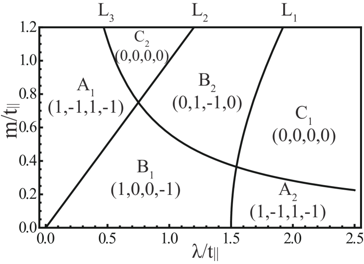
Figure 1: Phases with different spin Chern number patterns $(C_{s1},C_{s2},C_{s3},C_{s4})$ vs SO coupling strength $\lambda$ and the sub-lattice asymmetry parameter $m$. Due to the $s_{z}$ conservation and TR symmetry, only those of the four $s=\uparrow$ bands are shown. Phase boundaries $L_{1,2,3}$ satisfy the level crossing conditions located at $\Gamma$, $K$, and $K^{\prime}$, respectively. Their analytic expressions are $\lambda^{2}-m^{2}=(\frac{3}{4}t_{\parallel})^{2}$, $\lambda=m$, and $\lambda\,m=(\frac{3}{4}t_{\parallel})^{2}$, respectively. $L_{1}$ and $L_{3}$ intersect at $(\lambda,m)=(\frac{3}{4}(\sqrt{5}+2),\frac{3}{4}(\sqrt{5}-2))\approx(1.54,0.36)$, and $L_{2}$ and $L_{3}$ intersect at $(\lambda,m)=(\frac{3}{4},\frac{3}{4})$.

In this section, we study the topology of band structures after SO coupling $\lambda$ is turned on. Due to the $s_{z}$ conservation, the $Z_{2}$ topological class is augmented to the spin Chern class. Without loss of generality, we only use the pattern of Chern numbers of the sector $s=\uparrow$ to characterize the band topology, and that of the $s=\downarrow$ sector is just with an opposite sign. The Berry curvature for the $i$-th band is defined as

$$F_{i}(\vec{k})=\partial_{k_{x}}A_{y}(\vec{k})-\partial_{k_{y}}A_{x}(\vec{k})$$ (66)

in which the Berry connection is defined as $\vec{A}_{i}(\vec{k})=-i\langle\phi_{i}(\vec{k})|\vec{\nabla}_{k}|\phi_{i}(\vec{k})\rangle$. The spin Chern number of band $i$ can be obtained through the integral over the entire first Brillouin zone as

$$C_{s,i}=\frac{1}{2\pi}\int_{FBZ}dk_{x}dk_{y}F_{i}(\vec{k}_{x},\vec{k}_{y}).$$ (67)

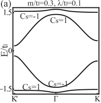
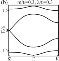
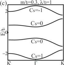
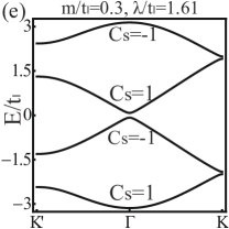
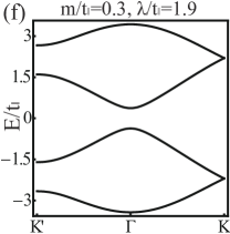
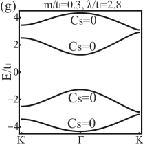
Figure 2: The spectra along the cut of $K^{\prime}$-$\Gamma$-$K$ in Brillouin zone. The spectra evolution is shown with fixed $m/t_{\parallel}=0.3$ and increasing $\lambda$ from 0.1 (a) to 2.8 (g), which passes phases $A_{1}$, $B_{1}$, $A_{2}$, and $C_{1}$. The pattern of spin-Chern numbers in the gapped states are marked. Parameters of (b), (d), and (f) are located at phase boundaries and gaps are closed at $K^{\prime}$, $\Gamma$, and $K$ points for (b), (d), and (f), respectively. Please note the appearance of single Dirac cones for the sector of spin-$\uparrow$, which is possible in 2D when two masses from sublattice asymmetry and SO coupling compete.

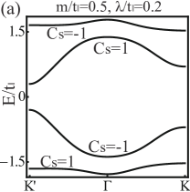
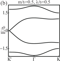
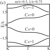
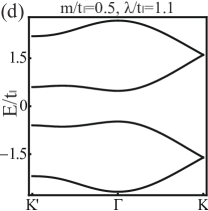
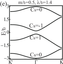
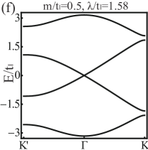
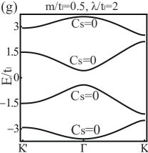
Figure 3: The same plot as in Fig. 2 but for the evolution with fixed $m/t_{\parallel}=0.5$ and increasing $\lambda$ from 0.2 (a) to 2 (g), which passes phases $A_{1}$, $B_{1}$, and $B_{2}$ and $C_{1}$. Gaps are closed at $K^{\prime}$, $K$, and $\Gamma$ points in (b), (d), and (f), respectively.

V.1 Band crossings at $\Gamma$, $K$ and $K^{\prime}$

We have performed the numerical integration for spin Chern numbers $(C_{s,1},C_{s,2},C_{s,3},C_{s,4})$ for $H_{\uparrow}(\vec{k})$ as presented in Fig. 1 based on Eq. (67). The phase boundary lines $L_{1,2,3}$ are associated with band touching, which occurs at high symmetry points $\Gamma$, $K$, and $K^{\prime}$, respectively. The momenta of these points are defined as $(0,0)$, $(\pm\frac{4\pi}{3\sqrt{3}},0)$. Since the dispersions of $H_{\uparrow}(\vec{k})$ are symmetric with respect to zero energy, the band crossing occurs either between bands 2 and 3 at zero energy, or between 1 and 2, 3 and 4 symmetrically with respect to zero energy.

We first check the crossing at the $\Gamma$-point. According to Eq. (16), the energies of the two middle levels are

$$E_{2,3}(\Gamma)=\pm\left(\lambda-\sqrt{m^{2}+\big{(}\frac{3}{2}t_{\parallel}\big{)}^{2}}\right).$$ (68)

The level crossing can only occur at zero energy with the hyperbolic condition

$$\lambda^{2}=m^{2}+\Big{(}\frac{3}{2}t_{\parallel}\Big{)}^{2},$$ (69)

which corresponds to line $L_{1}$ in Fig. 1.

The sublattice asymmetry parameter $m$ and SO coupling $\lambda$ are different mass generation mechanisms. The former breaks parity and contributes equally at $K$ and $K^{\prime}$, while the latter exhibits opposite signs. Their total effects superpose constructively or destructively at $K$ and $K^{\prime}$, respectively, as shown in the spectra of the two lower energy levels at $K$ and $K^{\prime}$. At $K^{\prime}=(-\frac{4\pi}{3\sqrt{3}},0)$, they are

$$E_{2,3}(K^{\prime})=\pm(\lambda-m),$$ (70)

and those at $K=(\frac{4\pi}{3\sqrt{3}},0)$ are

$$E_{1,4}(K) = \mp\sqrt{(m-\lambda)^{2}+\Big{(}\frac{3}{2}t_{\parallel}\Big{)}^{2}},$$

$$E_{2,3}(K) = \mp(m+\lambda).$$ (71)

Thus the level crossing at $K^{\prime}$ occurs at zero energy with the relation

$$\lambda=m,$$ (72)

which is line $L_{2}$ in Fig. 1. Similarly, the level crossing at $K$ occurs when $E_{2}(K)=E_{1}(K)$ leading to the condition

$$\lambda\,m=\Big{(}\frac{3}{4}t_{\parallel}\Big{)}^{2},$$ (73)

which is line $L_{3}$ in Fig. 1.

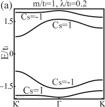
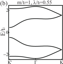
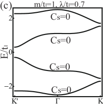
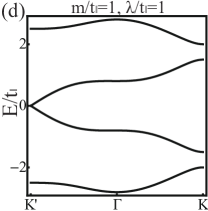
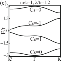
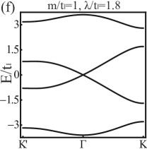
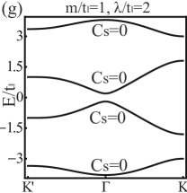
Figure 4: The same plot as in Fig. 2 but for the evolution fixing $m/t_{\parallel}=1$ and increasing $\lambda$ from 0.2 (a) to 2 (g), which passes phases $A_{1}$, $C_{2}$, and $B_{2}$ and $C_{1}$. Gaps are closed at $K^{\prime}$, $K$, and $\Gamma$ points in (b), (d), and (f), respectively.

V.2 Evolution of the topological band structures

The lattice asymmetry term $m$ by itself can open a gap at $K$ and $K^{\prime}$ in the absence of SO coupling. In this case, the gap value is $m$ at both $K$ and $K^{\prime}$. The lower two bands remain touched at the $\Gamma$ point with quadratic band touching. Nevertheless, the overall band structure remains nontopological.

The SO coupling $\lambda$ brings nontrivial band topology. Its competition with the lattice asymmetry results in a rich structure of band structure topology presented in Fig. 1, which are characterized by their pattern of spin Chern numbers. There are two phases characterized by the same spin Chern number pattern $(1,-1,1-1)$ marked as $A_{1}$ and $A_{2}$, respectively; two phases characterized by $(1,0,0,-1)$ marked as $B_{1}$ and $B_{2}$; and two trivial phases denoted as $C_{1}$ and $C_{2}$ $(0,0,0,0)$.

Even an infinitesimal value of $\lambda$ removes the quadratic band touching between the band 1 and 2, and brings nontrivial band topology. The line of $m=0$ corresponds to the situation investigated in the QAH insulator based on the $p_{x}$- and $p_{y}$-orbital bands in the honeycomb lattice Wu (2008b); Zhang et al. (2011). The current situation is a 2D topological insulator with $s_{z}$ conserved, which is just a double copy of the previous QAH model. At small values of $\lambda$, the system is in the $B_{1}$ phase. It enters the $A_{2}$ phase after crossing the line $L_{1}$ at $\lambda=\frac{3}{2}t_{\parallel}$.

If the system begins with a nonzero lattice asymmetry parameter $m$, it first enters the $A_{1}$. If we increase SO coupling strength $\lambda$ by fixing $m$ at different values, different band topology transitions appear. To further clarify these transitions, we plot the spectra evolutions with increasing $\lambda$ while fixing $m=0.3,0.5$, and 1 in Figs. 2,  3,  4, respectively. Only the spectra along the line cut from $K^{\prime}$ to $\Gamma$ to $K$ in the Brillouin zone are plotted. At small values of $m$ as shown in Fig. 2, the gap first closes at $K^{\prime}$, and then at $\Gamma$, and finally at $K$ with increasing $\lambda$. The sequence of phase transitions is $A_{1}\rightarrow B_{1}\rightarrow A_{2}\rightarrow C_{1}$. At intermediate values of $m$ shown in Fig. 3, the gap first closes at $K^{\prime}$, then at $K$, and finally at $\Gamma$ leading to a sequence of phase transitions $A_{1}\rightarrow B_{1}\rightarrow B_{2}\rightarrow C_{1}$. At large values of $m$ as shown in Fig. 4, the gap first closes at $K^{\prime}$, then at $K$, and finally at $\Gamma$. The sequence of phases is $A_{1}\rightarrow C_{2}\rightarrow B\rightarrow C_{1}$.

VI Reduced two-band models around band crossings

In order to further clarify topological band transitions, we derive the effective two-band Hamiltonians around the gap closing points ($\Gamma$, $K$, and $K^{\prime}$) respectively in this section.

Since the crossing at the $\Gamma$ point occurs at zero energy, we consider the middle two states. We construct the two bases as

$$|\phi_{2}(\vec{k})\rangle = \cos\frac{\alpha}{2}|\psi_{A,-}(\vec{k})\rangle+\sin\frac{\alpha}{2}|\psi_{B,-}(\vec{k})\rangle$$

$$|\phi_{3}(\vec{k})\rangle = -\sin\frac{\alpha}{2}|\psi_{A,+}(\vec{k})\rangle+\cos\frac{\alpha}{2}|\psi_{B,+}(\vec{k})\rangle,$$ (74)

where $\alpha=\arctan\frac{3t_{\parallel}}{2m}$. Right at the $\Gamma$ point, these two bases are the eigenvectors of the middle two bands with energies are $E_{2,3}(\Gamma)=\mp(\sqrt{m^{2}+(\frac{3}{2}t_{\parallel})^{2}}-\lambda)$, respectively. As $\lambda\rightarrow\sqrt{m^{2}+(\frac{3}{2}t_{\parallel})^{2}}$, we construct the low-energy Hamiltonian for $\vec{k}$ around the $\Gamma$ point by using $|\phi_{2,3}(\vec{k})\rangle$ as bases:

$$\left[\begin{array}[]{cc}\langle\phi_{2}|H|\phi_{2}\rangle&\langle\phi_{2}|H|\phi_{3}\rangle\\ \langle\phi_{3}|H|\phi_{2}\rangle&\langle\phi_{3}|H|\phi_{3}\rangle\end{array}\right]$$ (77)

$$= \left[\begin{array}[]{cc}-\lambda+\sqrt{m^{2}+(\frac{3}{2}t_{\parallel})^{2}}&\frac{3}{4}t_{\parallel}(k_{x}+ik_{y})\\ \frac{3}{4}t_{\parallel}(k_{x}-ik_{y})&\lambda-\sqrt{m^{2}+(\frac{3}{2}t_{\parallel})^{2}}\end{array}\right],\ \ \$$ (80)

which describes the band crossing of line $L_{1}$ in Fig. 1. The two-band effective model for the crossing at the $K^{\prime}$ point is just what we have constructed in Eq. (92). It describes the crossing at zero energy represented by line $L_{2}$ in Fig. 1.

As for the band crossing at the $K$ point, it occurs between band 1 and 2, and between 3 and 4 symmetrically with respect to zero energy ($B_{2}$, $C_{1}$, and $C_{2}$ phases). For simplicity, we only consider the effective two-band model at small values of $m$. In this case, the band crossing is described by line $L_{3}$ in Fig. 1 occurring at large values of $\lambda\gg m$. The on-site energy level splitting between the states of $(p_{+},\uparrow)$ and $(p_{-},\uparrow)$ is larger than the hopping integral $t_{\parallel}$, and each of them will develop a single band in the honeycomb lattice. The bands of $p_{\pm}$ orbitals lie symmetrically with respect to zero energy. Nevertheless, as shown in Refs. Wu, 2008b; Zhang et al., 2011, the interband coupling at the second-order perturbation level effectively generates the complex-valued next-nearest-neighbor hopping as in Haldane’s QAH model Haldane (1988). Our current situation is a TR double copy and thus it gives rise to the Kane-Mele model.

To describe the above physics, we only keep the $p_{+}$ orbitals on each site in the case of large values of $\lambda$. Then the terms of $h_{11}$, $h_{22}$, $h_{21}$, and $h_{12}$ in Eq. (7) become perturbations. By the second-order perturbation theory, we derive the low-energy Hamiltonian of $(p_{A,+}(\vec{k}),p_{B,+}(\vec{k}))$ bands as

$$\left[\begin{array}[]{cc}\langle\psi_{A+}|H|\psi_{A+}\rangle&\langle\psi_{A+}|H|\psi_{B_{+}}\rangle\\ \langle\psi_{B+}|H|\psi_{A+}\rangle&\langle\psi_{B+}|H|\psi_{B_{+}}\rangle\end{array}\right]$$ (83)

$$= \left[\begin{array}[]{cc}m+m_{H}(\vec{k})&-\frac{t_{\parallel}}{2}l^{*}(\vec{k})\\ -\frac{t_{\parallel}}{2}l(\vec{k})&-m-m_{H}(\vec{k})\end{array}\right],$$ (85)

where

$$m_{H}(\vec{k})=\frac{\sqrt{3}}{8}\frac{t^{2}_{\parallel}}{\lambda}\sin\eta_{s}(\vec{k}).$$ (86)

Around the $K$ point, $m_{H}(K)=-\frac{9}{16}\frac{t_{\parallel}^{2}}{\lambda}$. The band crossing occurs when $m+m_{H}(\vec{k})$ switches sign, which gives rise to line $L_{3}$ in Fig. 1.

The topological gap opens at the $K^{\prime}$ point between bands 2 and 3. According to Eq. (47), we only need to keep the right-bottom block for the construction of the low-energy two-band model. By expanding around the $K^{\prime}$ point, we have

$$\left[\begin{array}[]{cc}\langle A_{2}|H|A_{2}\rangle&\langle A_{2}|H|B_{2}\rangle\\ \langle B_{2}|H|A_{2}\rangle&\langle B_{2}|H|B_{2}\rangle\end{array}\right]$$ (89)

$$= \left[\begin{array}[]{cc}m-\lambda&-\frac{3}{4}t_{\parallel}(\delta k_{x}+i\delta k_{y})\\ -\frac{3}{4}t_{\parallel}(\delta k_{x}-i\delta k_{y})&-m+\lambda\end{array}\right],$$ (92)

where $\delta\vec{k}=\vec{k}-\vec{K}^{\prime}$, and thus the mass term is controlled by $m-\lambda$. For completeness, we also derive the effective two-band Hamiltonian for bands 2 and 3 around the $K$ point similarly, which yields the gap value $m+\lambda$. In the absence of lattice asymmetry, the gap values at $K$ and $K^{\prime}$ are both the SO coupling strength.

Now let us look more carefully at the eigen wave functions of the effective two-band Hamiltonian for bands 2 and 3 at $K^{\prime}$ and $K$ points and check their orbital angular momenta. The eigenstates are just $|A_{2}(K^{\prime})\rangle$ and $|B_{2}(K^{\prime})\rangle$ at $K^{\prime}$, and $|A_{2}(K)\rangle$, and $|B_{2}(K)\rangle$ at $K$. In the bases of Eq. (5), we express

$$|A_{2}(K^{\prime})\rangle=\left[\begin{array}[]{c}1\\ 0\\ 0\\ 0\end{array}\right],\ \ \,|B_{2}(K^{\prime})\rangle=\left[\begin{array}[]{c}0\\ 0\\ 0\\ 1\end{array}\right],$$ (101)

$$|A_{2}(K)\rangle=\left[\begin{array}[]{c}0\\ 0\\ 1\\ 0\end{array}\right],\ \ \,|B_{2}(K)\rangle=\left[\begin{array}[]{c}0\\ 1\\ 0\\ 0\end{array}\right].$$ (110)

All of them are the orbital angular momentum eigenstates with $L_{z}=\pm 1$. Considering this is the sector with $s=\uparrow$, the gap is just the atomic SO coupling strength $\lambda$ in the absence of the lattice asymmetry term $m$.

VII Large topological band gaps

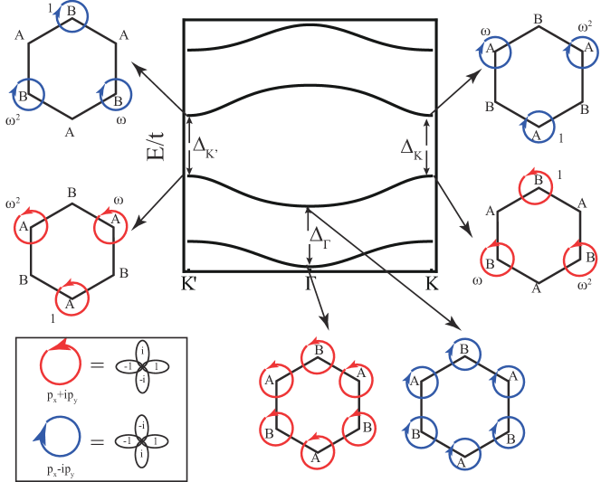
Figure 5: (Color online) The topological energy gap at the high symmetry $K^{\prime}$, $K$, and $\Gamma$ points for the $B_{1}$ phase, denoted $\Delta_{K^{\prime}}$, $\Delta_{K}$, and $\Delta_{\Gamma}$ respectively. $\Delta_{K^{\prime}}=\Delta_{K}=\Delta_{\Gamma}=2\lambda$ in the absence of lattice asymmetry. The corresponding real space orbital configurations of the eigenstates are of $p_{x}\pm ip_{y}$ type ($L_{z}=\pm 1$). We denote the orbital angular momentum $L_{z}=\pm 1$ eigenstates as red (blue) counterclockwise (clockwise) circles, as shown in the inset. At the $K^{\prime}(K)$ point, the eigenstate for band 2 is of the $p_{x}+ip_{y}$ type completely located at the A(B) sublattice, while for band 3 the eigenstate is of the $p_{x}-ip_{y}$ type at the B(A) sublattice. The phase factor for each site in the hexagonal plquette is $\omega=e^{i\frac{2}{3}\pi}$. At the $\Gamma$ point, the eigenstates for band 1 and 2 are both superpositions of the wave functions at $A$ and $B$ sublattices, but with opposite orbital angular momentum.

The most striking feature of the these $p_{x}$-$p_{y}$ systems is the large topological band gap at $K^{\prime}$, $K$, and $\Gamma$ points. In this section, we analyze the origin of large topological band gaps at these $k$ points in the $B_{1}$ phase (quantum spin Hall (QSH) phase, $\lambda>m$). For the case of a single-component fermion QAH model studied in Ref. Wu, 2008b, it has been analyzed that the gap values at the $\Gamma$, $K$, and $K^{\prime}$ points are just the on-site rotation angular velocity $\Omega$ in the absence of the lattice asymmetry term. The situation in this paper is a TR invariant double copy of the previously single component case, and thus the role of of $\Omega$ is replaced by the on-site atomic SO coupling strength $\lambda$.

At the $K^{\prime}$ point, according to Eq. (110), the eigenstates for the bands 2,3 are orbital angular momentum eigenstates with $L_{z}=\pm 1$. The energy and corresponding eigenstates for bands 2 and 3 are

$$E_{2}(K^{\prime}) = m-\lambda,\quad|\phi_{2}(K^{\prime})\rangle=|\psi_{A,+}(K^{\prime})\rangle,$$

$$E_{3}(K^{\prime}) = \lambda-m,\quad|\phi_{3}(K^{\prime})\rangle=|\psi_{B,-}(K^{\prime})\rangle,$$

$$\Delta_{K^{\prime}} = 2(\lambda-m).$$ (111)

As shown in Fig. 5, the eigenstate for band 2 has $L_{z}=+1$ with the energy $m-\lambda$, which is of $p_{x}+ip_{y}$ type, and its wave function is totally on the $A$ sublattice. In contrast, the eigenstate for band 3 has $L_{z}=-1$ with the energy $\lambda-m$. It is of the $p_{x}-ip_{y}$ type whose wave function completely distributes on the $B$ sublattice. The topological band gap is thus $2(\lambda-m)$. If the sublattice asymmetry term vanishes, i.e., $m=0$, the band gap is just $2\lambda$.

Obviously, the atomic on-site SO coupling strength $\lambda$ directly contributes to the topological band gap, leading to a large band splitting. It is because at the $K^{\prime}$ point, the eigenstates of the system are also $L_{z}$ eigenstates, which means the topological band gap is the eigenenergy difference between the SO coupling term $s_{z}L_{z}$ for $L_{z}=\pm 1$. It is easy to generalize the analysis to the $K$ point similarly.

At the $\Gamma$ point, the Hamiltonian $H(\vec{k})$ preserves all the rotation symmetries of the system, and thus the SO coupling term $s_{z}L_{z}$ commutes with $H(\vec{k})$. The eigenstates simultaneously diagonalize the SO coupling term and $H(\vec{k})$. The energy and corresponding eigenstates for bands 1 and 2 at the $\Gamma$ point are

$$E_{1}(\Gamma) = -\lambda-\sqrt{m^{2}+(\frac{3}{2}t_{\parallel})^{2}},$$

$$|\phi_{1}(\Gamma)\rangle = \sin\frac{\alpha}{2}|\psi_{A,+}(\Gamma)\rangle+\cos\frac{\alpha}{2}|\psi_{B,+}(\Gamma)\rangle,$$

$$E_{2}(\Gamma) = \lambda-\sqrt{m^{2}+(\frac{3}{2}t_{\parallel})^{2}},$$

$$|\phi_{2}(\Gamma)\rangle = \cos\frac{\alpha}{2}|\psi_{A,-}(\Gamma)\rangle+\sin\frac{\alpha}{2}|\psi_{B,-}(\Gamma)\rangle,$$

$$\Delta_{\Gamma} = 2\lambda.$$ (112)

The eigenstates for bands 1,2 are the superpositions of wave functions on both the $A$ and $B$ sublattices. However, for band 1, the eigenstate is an $L_{z}=-1$ eigenstate, and the eigenstate for band 2 is an $L_{z}=1$ eigenstate (see Fig. 5). As a result, the topological band gap $\Delta_{\Gamma}$ is the energy difference of the SO coupling term $s_{z}L_{z}$, which is $2\lambda$.

We discuss the dependence of the topological gap values on SO coupling strength in the $B_{1}$ phase. Let us first consider the gap between the lowest two bands. For the case without lattice asymmetry, i.e., $m/t_{\parallel}=0$, in the weak and intermediate regimes of the SO coupling strength $0<\lambda/t_{\parallel}<3/(4\sqrt{2})$, the minimal gap is located at the $\Gamma$ point as shown in Fig. 2(b). In typical solid state systems, $\lambda$ lies in these regimes, and thus, typically, the topological gap can approach up to $2\lambda=3/(2\sqrt{2})t_{\parallel}$, which is a very large gap. If $\lambda$ further increases, then the minimal gap shifts from the $\Gamma$ point to the $K$ points, and the value of the gap shrinks as $\lambda$ increases. Similarly, consider the topological gap between the middle two bands, and for parameters $m/t_{\parallel}=0$: as long as the SO coupling strength is in the $B_{1}$ phase, the minimal gap is located at the $K(K^{\prime})$ point, which can approach up to $2\lambda=3\,t_{\parallel}$.

VIII Quantum Anomalous Hall State

In this section, we add the Néel antiferromagnetic exchange field term [Eq. (4)] to the Hamiltonian. This term gives rise to another mass generation mechanism. Together with the atomic SO coupling term of $L_{z}\sigma_{z}$, and the sublattice asymmetry term [Eq. (LABEL:eq:m)] discussed before, we can drive the system to a QAH state. A similar mechanism was also presented in the single-orbital honeycomb lattice Liang et al. (2013), and here we generalize it to the $p_{x}$-$p_{y}$-orbital systems.

We consider the gap opening at the $K$ and $K^{\prime}$ points, and assume that bands 1 and 2 are filled. In the absence of the Néel term [Eq. (4)], the system is in the trivially gapped phase $A_{1}$ at $m>\lambda$, and in the QSH phase $B_{1}$ at $\lambda>m$.

Let us start with the QSH phase $B_{1}$ with $\lambda>m>0$, and gradually turn on the Néel exchange magnitude $n>0$. The energy levels for different spin sectors at the $K^{\prime}$ and $K$ points for the middle two bands are

$$E_{2,3,\uparrow}(K^{\prime}) = \mp(\lambda-m-n),$$

$$E_{2,3,\downarrow}(K^{\prime}) = \mp(\lambda+m-n),$$

$$E_{2,3,\uparrow}(K) = \mp(\lambda+m+n),$$

$$E_{2,3,\downarrow}(K) = \mp(\lambda-m+n).$$ (113)

The gap will not close for both spin-$\uparrow$ and spin-$\downarrow$ sectors at the $K$ point with increasing $n$, and thus we focus on the band crossing at the $K^{\prime}$ point. At this point, the first band crossing occurs in the spin-$\uparrow$ sector at $n=\lambda-m$, which changes the spin-$\uparrow$ sector into the topologically trivial regime. Meanwhile, the spin-$\downarrow$ sector remains topologically nontrivial, and thus the system becomes a QAH state. If we further increase $n$, the second band crossing occurs in the spin-$\downarrow$ sector at $n=\lambda+m$, at which the spin-$\downarrow$ sector also becomes topologically trivial. In this case, the entire system is a trivial band insulator. The QAH state can be realized for $\lambda-m<n<\lambda+m$. The band crossing diagrams are shown in Fig. 6(a).

Similarly, we start from the $A_{1}$ trivially gapped phase ($0<\lambda<m$), and gradually turn on the Néel exchange field $n$. The middle two energy levels for both spin sectors at the $K^{\prime}$ and $K$ points are

$$E_{2,3,\uparrow}(K^{\prime}) = \mp(m-\lambda+n),$$

$$E_{2,3,\downarrow}(K^{\prime}) = \mp(m+\lambda-n),$$

$$E_{2,3,\uparrow}(K) = \mp(m+\lambda+n),$$

$$E_{2,3,\downarrow}(K) = \mp(m-\lambda-n).$$ (114)

In this case, the spin-$\uparrow$ sector remains in the trivially gapped phase with increasing $n$, since there is no band inversion in this sector [see Fig. 6(b)]. The first band crossing occurs in the spin-$\downarrow$ sector at the $K$ point when $n=m-\lambda$, rendering this sector topologically nontrivial, and then the whole system goes into a QAH phase. The second band inversion occurs at the $K^{\prime}$ point also in the spin-$\downarrow$ sector at $n=\lambda+m$. Now the spin-$\downarrow$ sector is back into a topologically trivial phase, and the whole system is a trivial band insulator for $n>\lambda+m$. Similarly to the previous case, the QAH phase is realized at $-\lambda+m<n<\lambda+m$.

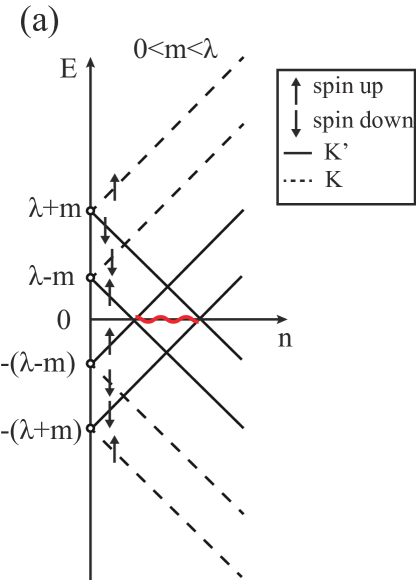
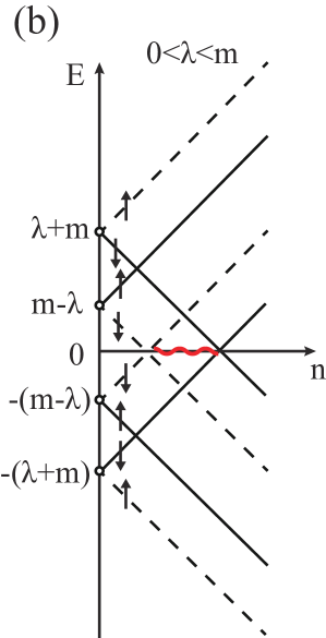
Figure 6: (Color online) Diagrams of the energy level crossing with increasing antiferromagnetic exchange field strength $n$ for two parameter regimes (a) $0<m<\lambda$ and (b) $0<\lambda<m$. Red wavy lines indicate the range of $n$ for the system to be in a QAH phase ($|\lambda-m|<n<\lambda+m$).

There are three gap parameters in our model, the spin-orbit coupling $\lambda$, the sublattice asymmetry term $m$, and the Néel exchange field $n$. Combining the two situations discussed above, we summarize the condition for the appearance of the QAH state as follows:

$$|\lambda-m|<n<\lambda+m,$$ (115)

which is also equivalent to $|m-n|<\lambda<m+n$, or $|\lambda-n|<m<\lambda+n$. In other words, the three gap parameters $\lambda$, $m$, and $n$ can form a triangle. For the buckled honeycomb lattices, the A and B sublattices are at different heights. The Néel exchange field $n$ can be generated by attaching two ferromagnetic substrates with opposite magnetizations to the two surfaces, and the sublattice asymmetry term $m$ can also be generated if the contacts with these two substrates are asymmetric. In the parameter regime for the QAH state, it is easy to check that the maximal topological gap is the minimum of $\lambda$ and $m$.

IX Conclusions and Outlooks

In summary, we have presented a minimal model to describe the 2D topological insulator states in the honeycomb lattice which have been recently proposed in the literature. The $p_{x}$ and $p_{y}$ orbitals are the key, and thus their properties are dramatically different from those in graphene. The atomic level SO coupling directly contributes to the topological gap opening, and thus the gap can be large. Due to the conservation of $s_{z}$, the band structures are a TR invariant doublet of the previously investigated QAHE based on the $p$ orbital in the honeycomb lattice. The band topology is described by the spin Chern numbers. Both sublattice asymmetry and the on-site SO coupling can open the gap, and their competition leads to a rich structure of topological band insulating phases. Due to the underlying structure of Clifford algebra, the energy spectra and eigen wave functions can be obtained analytically. Also, the transition lines among different topological insulators are also analytically obtained. Low-energy two-band models are constructed around band crossings. Furthermore, with the help of the Néel antiferromagnetic exchange field, the model can enter into a QAH phase. This work provides a useful platform for further exploring interaction and topological properties in such systems.

In addition to a class of solid state materials, the model constructed in this article can, in principle, also be realized in ultracold-atom optical lattices. For example, in previous papers by one of the authors and his collaborators (Refs. Wu, 2008a and Zhang et al., 2011), the quantum anomalous Hall models were proposed for spinless fermions of the $p_{x}/p_{y}$ bands in the honeycomb optical lattices. By this technique, each optical site is rotating around its own center, which can be modeled as an orbital Zeeman term. The quantum spin Hall model of Eqs. (1) and (2) is a time-reversal invariant double of the anomalous quantum Hall model, which in principle can be realized by the spin-dependent on-site rotations of the honeycomb lattice, i.e., the rotation angular velocities for spin-$\uparrow$ and spin-$\downarrow$ fermions are opposite to each other. This is essentially a spin-orbit coupling term $L_{z}\,S_{z}$ and the rotation angular velocity plays the role of spin-orbit coupling strength. In order to observe the topological phase, we need the fermions population to fill the $p$-orbital bands. Then, the phase diagram will be the same as in Fig.1, by replacing the spin-orbit coupling strength with the magnitude of the angular velocity.

Note added Near the completion of this work, we became aware of the work Ref. Liu et al., in which the low energy effective model of the 2D topological insulators on honeycomb lattice are also constructed.