Parametrizing the moduli space of curves and applications to smooth plane quartics over finite fields

Abstract.

We study new families of curves that are suitable for efficiently parametrizing their moduli spaces. We explicitly construct such families for smooth plane quartics in order to determine unique representatives for the isomorphism classes of smooth plane quartics over finite fields. In this way, we can visualize the distributions of their traces of Frobenius. This leads to new observations on fluctuations with respect to the limiting symmetry imposed by the theory of Katz and Sarnak.

1. Introduction

One of the central notions in arithmetic geometry is the (coarse) moduli space of curves of a given genus $g$, denoted $\mathsf{M}_{g}$. These are algebraic varieties whose geometric points classify these curves up to isomorphism. The main difficulty when dealing with moduli spaces – without extra structure – is the non-existence of universal families, whose construction would allow one to explicitly write down the curve corresponding to a point of this space. Over finite fields, the existence of a universal family would lead to optimal algorithms to write down isomorphism classes of curves. Having these classes at one’s disposal is useful in many applications. For instance, it serves for constructing curves with many points using class field theory [32] or for enlarging the set of curves useful for pairing-based cryptography as illustrated in genus $2$ by [9, 14, 33]. More theoretically, it was used in [5] to compute the cohomology of moduli spaces. We were ourselves drawn to this subject by the study of Serre’s obstruction for smooth plane quartics (see Section 5.4).

The purpose of this paper is to introduce three substitutes for the notion of a universal family. The best replacement for a universal family seems to be that of a representative family, which we define in Section 2. This is a family of curves $\mathcal{C}\to\mathcal{S}$ whose points are in natural bijection with those of a given subvariety $S$ of the moduli space. Often the scheme $\mathcal{S}$ turns out to be isomorphic to $S$, but the notion is flexible enough to still give worthwhile results when this is not the case. Another interesting feature of these families is that they can be made explicit in many cases when $S$ is a stratum of curves with a given automorphism group. We focus here on the case of non-hyperelliptic genus $3$ curves, canonically realized as smooth plane quartics.

The overview of this paper is as follows. In Section 2 we introduce and study three new notions of families of curves. We indicate the connections with known constructions from the literature. In Proposition 2.3 and Proposition 2.4, we also uncover a link between the existence of a representative family and the question of whether the field of moduli of a curve is a field of definition. In Section 3 we restrict our considerations to the moduli space of smooth plane quartics. After a review of the stratification of this moduli space by automorphism groups, our main result in this section is Theorem 3.3. There we construct representative families for all but the two largest of these strata by applying the technique of Galois descent. For the remaining strata we improve on the results in the literature by constructing families with fewer parameters, but here much room for improvement remains. In particular, it would be nice to see an explicit representative (and in this case universal) family over the stratum of smooth plane quartics with trivial automorphism group.

Parametrizing by using our families, we get one representative curve per $\bar{k}$-isomorphism class. Section 4 refines these into $k$-isomorphism classes by constructing the twists of the corresponding curves over finite fields $k$. Finally, Section 5 concludes the paper by describing the implementation of our enumeration of smooth plane quartics over finite fields, along with the experimental results obtained on distributions of traces of Frobenius for these curves over $\mathbb{F}_{p}$ with $11\leq p\leq 53$. In order to obtain exactly one representative for every isomorphism class of curves, we use the previous results combined with an iterative strategy that constructs a complete database of such representatives by ascending up the automorphism strata.

Notations. Throughout, we denote by $k$ an arbitrary field of characteristic $p\geq 0$, with algebraic closure $\overline{k}$. We use $K$ to denote a general algebraically closed field. By $\zeta_{n}$, we denote a fixed choice of $n$-th root of unity in $\overline{k}$ or $K$; these roots are chosen in such a way to respect the standard compatibility conditions when raising to powers. Given $k$, a curve over $k$ will be a smooth and proper absolutely irreducible variety of dimension $1$ and genus $g>1$ over $k$.

In agreement with [24], we keep the notation $\mathbf{C}_{n}$ (resp. $\mathbf{D}_{2n}$, resp. $\mathbf{A}_{n}$, resp. $\mathbf{S}_{n}$) for the cyclic group of order $n$ (resp. the dihedral group of order $2n$, resp. the alternating group of order $n!/2$, resp. the symmetric group of order $n!$). We will also encounter $\mathbf{G}_{16}$, a group of $16$ elements that is a direct product $\mathbf{C}_{4}\times\mathbf{D}_{4}$, $\mathbf{G}_{48}$, a group of $48$ elements that is a central extension of $\mathbf{A}_{4}$ by $\mathbf{C}_{4}$, $\mathbf{G}_{96}$, a group of $96$ elements that is a semidirect product $(\mathbf{C}_{4}\times\mathbf{C}_{4})\rtimes\mathbf{S}_{3}$ and $\mathbf{G}_{168}$, which is a group of $168$ elements isomorphic to $\operatorname{PSL}_{2}(\mathbb{F}_{7})$.

Acknowledgments

We would like to thank Jonas Bergström, Bas Edixhoven, Everett Howe, Frans Oort and Matthieu Romagny for their generous help during the writing of this paper. Also, we warmly thank the anonymous referees for carefully reading this work and for suggestions.

2. Families of curves

Let $g>1$ be an integer, and let $k$ be a field of characteristic $p=0$ or $p>2g+1$. For $\mathcal{S}$ a scheme over $k$, we define a curve of genus $g$ over $\mathcal{S}$ to be a morphism of schemes $\mathcal{C}\rightarrow\mathcal{S}$ that is proper and smooth with geometrically irreducible fibers of dimension $1$ and genus $g$. Let $\mathsf{M}_{g}$ be the coarse moduli space of curves of genus $g$ whose geometric points over algebraically closed extensions $K$ of $k$ correspond with the $K$-isomorphism classes of curves $C$ over $K$.

We are interested in studying the subvarieties of $\mathsf{M}_{g}$ where the corresponding curves have an automorphism group isomorphic with a given group. The subtlety then arises that these subvarieties are not necessarily irreducible. This problem was also mentioned and studied in [26], and resolved by using Hurwitz schemes; but in this section we prefer another way around the problem, due to Lønsted in [25].

In [25, Sec.6] the moduli space $\mathsf{M}_{g}$ is stratified in a finer way, namely by using ‘rigidified actions’ of automorphism groups. Given an automorphism group $G$, Lønsted defines subschemes of $\mathsf{M}_{g}$ that we shall call strata. Let $\ell$ be a prime different from $p$, and let $\Gamma_{\ell}=\operatorname{Sp}_{2g}(\mathbb{F}_{\ell})$. Then the points of a given stratum $S$ correspond to those curves $C$ for which the induced embedding of $G$ into the group ($\cong\Gamma_{\ell}$) of polarized automorphisms of $\operatorname{Jac}(C)[\ell]$ is $\Gamma_{\ell}$-conjugate to a given group. Combining [18, Th.1] with [25, Th.6.5] now shows that under our hypotheses on $p$, such a stratum is a locally closed, connected and smooth subscheme of $\mathsf{M}_{g}$. If $k$ is perfect, such a connected stratum is therefore defined over $k$ if only one rigidification is possible for a given abstract automorphism group. As was also observed in [26], this is not always the case; and as we will see in Remark 3.2, in the case of plane quartics these subtleties are only narrowly avoided.

We return to the general theory. Over the strata $S$ of $\mathsf{M}_{g}$ with non-trivial automorphism group, the usual notion of a universal family (as in [28, p.25]) is of little use. Indeed, no universal family can exist on the non-trivial strata; by [1, Sec.14], $S$ is a fine moduli space (and hence admits a universal family) if and only if the automorphism group is trivial. In the definition that follows, we weaken this notion to that of a representative family. While such families coincide with the usual universal family on the trivial stratum, it will turn out (see Theorem 3.3) that they can also be constructed for the strata with non-trivial automorphism group. Moreover, they still have sufficiently strong properties to enable us to effectively parametrize the moduli space.

Definition 2.1.

Let $S\subset\mathsf{M}_{g}$ be a subvariety of $\mathsf{M}_{g}$ that is defined over $k$. Let $\mathcal{C}\rightarrow\mathcal{S}$ be a family of curves whose geometric fibers correspond to points of the subvariety $S$, and let $f_{\mathcal{C}}:\mathcal{S}\to S$ be the associated morphism.

1. The family $\mathcal{C}\rightarrow\mathcal{S}$ is geometrically surjective (for $S$) if the map $f_{\mathcal{C}}$ is surjective on $K$-points for every algebraically closed extension $K$ of $k$.

2. The family $\mathcal{C}\rightarrow\mathcal{S}$ is arithmetically surjective (for $S$) if the map $f_{\mathcal{C}}$ is surjective on $k^{\prime}$-points for every finite extension $k^{\prime}$ of $k$.

3. The family $\mathcal{C}\rightarrow\mathcal{S}$ is quasifinite (for $S$) if it is geometrically surjective and $f_{\mathcal{C}}$ is quasifinite.

4. The family $\mathcal{C}\rightarrow\mathcal{S}$ is representative (for $S$) if $f_{\mathcal{C}}$ is bijective on $K$-points for every algebraically closed extension $K$ of $k$.

Remark 2.2.

A family $\mathcal{C}\rightarrow\mathcal{S}$ is geometrically surjective if and only if the corresponding morphism of schemes $\mathcal{S}\to S$ is surjective.

Due to inseparability issues, the morphism $f_{\mathcal{C}}$ associated to a representative family need not induce bijections on points over arbitrary extensions of $k$.

Note that if a representative family $\mathcal{S}$ is absolutely irreducible, then since $S$ is normal, we actually get that $f_{\mathcal{C}}$ is an isomorphism by Zariski’s Main Theorem. However, there are cases where we were unable to find such an $\mathcal{S}$ given a stratum $S$ (see Remark 3.4).

The notions of being geometrically surjective, quasifinite and representative are stable under extension of the base field $k$. On the other hand, being arithmetically surjective can strongly depend on the base field, as for example in Proposition 3.5.

To prove that quasifinite families exist, one typically considers the universal family over $\mathsf{M}_{g}^{(\ell)}$ (the moduli space of curves of genus $g$ with full level-$\ell$ structure, for a prime $\ell>2$ different from $p$, see [1, Th.13.2]). This gives a quasifinite family over $\mathsf{M}_{g}$ by the forgetful (and in fact quotient) map $\mathsf{M}_{g}^{(\ell)}\to\mathsf{M}_{g}$ that we will denote $\pi_{\ell}$ when using it in our constructions below.

Let $K$ be an algebraically closed extension of $k$. Given a curve $C$ over $K$, recall that an intermediate field $k\subset L\subset K$ is a field of definition of $C$ if there exists a curve $C_{0}/L$ such that $C_{0}$ is $K$-isomorphic to $C$. The concept of representative families is related with the question of whether the field of moduli $\mathbf{M}_{C}$ of the curve $C$, which is by definition the intersection of the fields of definition of $C$, is itself a field of definition. Since we assumed that $p>2g+1$ or $p=0$, the field $\mathbf{M}_{C}$ then can be recovered more classically as the residue field of the moduli space $\mathsf{M}_{g}$ at the point $[C]$ corresponding to $C$ by [34, Cor.1.11]. This allows us to prove the following.

Proposition 2.3.

Let $S$ be a subvariety of $\mathsf{M}_{g}$ defined over $k$ that admits a representative family $\mathcal{C}\to\mathcal{S}$. Let $C$ be a curve over an algebraically closed extension $K$ of $k$ such that the point $[C]$ of $\mathsf{M}_{g}(K)$ belongs to $S$. Then $C$ descends to its field of moduli $\mathbf{M}_{C}$. In case $k$ is perfect and $K=\overline{k}$, then $C$ even corresponds to an element of $\mathcal{S}(\mathbf{M}_{C})$.

Proof.

First we consider the case where $k=\mathbf{M}_{C}$ and $K$ is a Galois extension of $k$. Let $x\in\mathcal{S}(K)$ be the preimage of $[C]$ under $f_{\mathcal{C}}$. For every $\sigma\in\operatorname{Gal}(K/k)$ it makes sense to consider $x^{\sigma}\in\mathcal{S}(K)$, since the family $\mathcal{C}$ is defined over $k$. Now since $f_{\mathcal{C}}$ is defined over $k$, we get $f_{\mathcal{C}}(x)=f_{\mathcal{C}}(x^{\sigma})=s$. By uniqueness of the representative in the family, we get $x=x^{\sigma}$. Since $\sigma$ was arbitrary and $K/k$ is Galois, we therefore have $x\in\mathcal{S}(k)$, which gives a model for $C$ over $k$ by taking the corresponding fiber for the family $\mathcal{C}\to\mathcal{S}$. This already proves the final statement of the proposition.

Since the notion of being representative is stable under changing the base field $k$, the argument in the Galois case gives us enough leverage to treat the general case (where $K/k$ is possibly transcendental or inseparable) by appealing to [20, Th.1.6.9]. ∎

Conversely, we have the following result. A construction similar to it will be used in the proof of Theorem 3.3.

Proposition 2.4.

Let $S$ be a stratum defined over a field $k$. Suppose that for every finite Galois extension $F\supset E$ of field extensions of $k$, the field of moduli of the curve corresponding to a point in $S(E)$ equals $E$. Then there exists a representative family $\mathcal{C}_{U}\to U$ over a dense open subset of $S$. If $k$ is perfect, this family extends to a possibly disconnected representative family $\mathcal{C}\to\mathcal{S}$ for the stratum $S$.

Proof.

Let $\eta$ be the generic point of $S$ and again let $\pi_{\ell}:\mathsf{M}_{g}^{(\ell)}\to\mathsf{M}_{g}$ be the forgetful map obtained by adding level structure at a prime $\ell>2$ different from $p$. Note that as a quotient by a finite group, $\pi_{\ell}$ is a finite Galois cover. Let $\nu$ be a generic point in the preimage of $\eta$ by $\pi_{\ell}$ and $\mathcal{C}\to\nu$ be the universal family defined over $k(\nu)$. By definition the field of moduli $\mathbf{M}_{\mathcal{C}}$ is equal to $k(\nu)$ and as $k(\nu)$ is a field of definition there exists a family $\mathcal{C}_{0}\to k(\nu)$ geometrically isomorphic to $\mathcal{C}$. Since $k(\nu)\supset k(\eta)$ is a Galois extension, we can argue as in the proof of Proposition 2.3 to descend to $k(\eta)$, and hence by a spreading-out argument we can conclude that $\mathcal{C}_{0}$ is a representative family on a dense open subset $U$ of $S$. Proceeding by induction over the (finite) union of the Galois conjugates of the finitely many irreducible components of the complement of $U$, which is again defined over $k$, one obtains the second part of the proposition. ∎

Whereas the universal family $\mathcal{C}\to\mathsf{M}_{g}^{(\ell)}$ is sometimes easy to construct, it seems hard to work out $\mathcal{C}_{0}$ directly by explicit Galois descent; the Galois group of the covering $\mathsf{M}_{g}^{(\ell)}\to\mathsf{M}_{g}$ is $\operatorname{Sp}_{2g}(\mathbb{F}_{\ell})$, which is a group of large cardinality $\ell^{g^{2}}\prod_{i=1}^{g}(\ell^{2i}-1)$ whose quotient by its center is simple. Moreover, for enumeration purposes, it is necessary for the scheme $\mathcal{S}$ to be as simple as possible. Typically one would wish for it to be rational, as fortunately turns out always to be the case for plane quartics. On the other hand, for moduli spaces of general type that admit no rational curves, such as $\mathsf{M}_{g}$ with $g>23$, there does not even exist a rational family of curves with a single parameter [16].

3. Families of smooth plane quartics

3.1. Review : automorphism groups

Let $C$ be a smooth plane quartic over an algebraically closed field $K$ of characteristic $p\geq 0$. Then since $C$ coincides up to a choice of basis with its canonical embedding, the automorphism $\operatorname{Aut}(C)$ can be considered as a conjugacy class of subgroups $\operatorname{PGL}_{3}(K)$ (and in fact of $\operatorname{GL}_{3}(K)$) by using the action on its non-zero differentials.

The classification of the possible automorphism groups of $C$ as subgroup of $\operatorname{PGL}_{3}(K)$, as well as the construction of some geometrically complete families, can be found in several articles, such as [17, 2.88], [39, p.62], [26], [3] and [8] (in chronological order), in which it is often assumed that $p=0$. We have verified these results independently, essentially by checking which finite subgroups of $\operatorname{PGL}_{3}(K)$ (as classified in [20, Lem.2.3.7]) can occur for plane quartics. It turns out that the classification in characteristic $0$ extends to algebraically closed fields $K$ of prime characteristic $p\geq 5$. In the following theorem, we do not indicate the open non-degeneracy conditions on the affine parameters, since we shall not have need of them.

Theorem 3.1.

Let $K$ be an algebraically closed field whose characteristic $p$ satisfies $p=0$ or $p\geq 5$. Let $C$ be a genus $3$ non-hyperelliptic curve over $K$. The following are the possible automorphism groups of $C$, along with geometrically surjective families for the corresponding strata:

1. $\{1\}$, with family $q_{4}(x,y,z)=0,$ where $q_{4}$ is a homogeneous polynomial of degree $4$;

2. $\mathbf{C}_{2}$, with family $x^{4}+x^{2}q_{2}(y,z)+q_{4}(y,z)=0$, where $q_{2}$ and $q_{4}$ are homogeneous polynomials in $y$ and $z$ of degree $2$ and $4$;

3. $\mathbf{D}_{4}$, with family $x^{4}+y^{4}+z^{4}+rx^{2}y^{2}+sy^{2}z^{2}+tz^{2}x^{2}=0$;

4. $\mathbf{C}_{3}$, with family $x^{3}z+y(y-z)(y-rz)(y-sz)=0$;

5. $\mathbf{D}_{8}$, with family $x^{4}+y^{4}+z^{4}+rx^{2}yz+sy^{2}z^{2}=0$;

6. $\mathbf{S}_{3}$, with family $x(y^{3}+z^{3})+y^{2}z^{2}+rx^{2}yz+sx^{4}=0$;

7. $\mathbf{C}_{6}$, with family $x^{3}z+y^{4}+ry^{2}z^{2}+z^{4}=0$;

8. $\mathbf{G}_{16}$, with family $x^{4}+y^{4}+z^{4}+ry^{2}z^{2}=0$;

9. $\mathbf{S}_{4}$, with family $x^{4}+y^{4}+z^{4}+r(x^{2}y^{2}+y^{2}z^{2}+z^{2}x^{2})=0$;

10. $\mathbf{C}_{9}$, represented by the quartic $x^{3}y+y^{3}z+z^{4}=0$;

11. $\mathbf{G}_{48}$, represented by the quartic $x^{4}+(y^{3}-z^{3})z=0$;

12. $\mathbf{G}_{96}$, represented by the Fermat quartic $x^{4}+y^{4}+z^{4}=0$;

13. (if $p\neq 7$) $\mathbf{G}_{168}$, represented by the Klein quartic $x^{3}y+y^{3}z+z^{3}x=0$.

The families in Theorem 3.1 are geometrically surjective. Moreover, they are irreducible and quasifinite (as we will see in the proof of Theorem 3.3) for all groups except the trivial group and $\mathbf{C}_{2}$. The embeddings of the automorphism group of these curves into $\operatorname{PGL}_{3}(K)$ can be found in Theorem A.1 in Appendix A. Because of the irreducibility properties mentioned in the previous paragraph, each of the corresponding subvarieties serendipitously describes an actual stratum in the moduli space $\mathsf{M}_{3}^{\textrm{nh}}\subset\mathsf{M}_{3}$ of genus $3$ non-hyperelliptic curves as defined in Section 2 (see Remark 3.2 below). From the descriptions in A.1, one derives the inclusions between the strata indicated in Figure 1, as also obtained in [39, p.65].

Figure 1. Automorphism groups

Remark 3.2.

As promised at the beginning of Section 2, we now indicate two different possible rigidifications of an action of a finite group on plane quartics. Consider the group $\mathbf{C}_{3}$. Up to conjugation, this group can be embedded into $\operatorname{PGL}_{3}(K)$ in exactly two ways; as a diagonal matrix with entries proportional to $(\zeta_{3},1,1)$ or $(\zeta_{3}^{2},\zeta_{3},1)$. This gives rise to two rigidifications in the sense of Lønsted.

While for plane curves of sufficiently high degree, this indeed leads to two families with generic automorphism group $\mathbf{C}_{3}$, the plane quartics admitting the latter rigidification always admit an extra involution, so that the full automorphism group contains $\mathbf{S}_{3}$. It is this fortunate phenomenon that still makes a naive stratification by automorphism groups possible for plane quartics. For the same reason, the stratum for the group $\mathbf{S}_{3}$ is not included in that for $\mathbf{C}_{3}$, as is claimed incorrectly in [3].

3.2. Construction of representative families

We now describe how to apply Galois descent to extensions of function fields to determine representative families for the strata in Theorem 3.1 with $|G|>2$. By Proposition 2.3, this shows that the descent obstruction always vanishes for these strata.

Our constructions lead to families that parametrize the strata much more efficiently; for the case $\mathbf{D}_{4}$, the family in Theorem 3.1 contains as much as $24$ distinct fibers isomorphic with a given curve. Moreover, by Proposition 2.3, in order to write down a complete list of the $\overline{k}$-isomorphism classes of smooth plane quartics defined over a perfect field $k$ we need only consider the $k$-rational fibers of the new families.

As in Theorem 3.1, we do not specify the condition on the parameters that avoid degenerations (i.e. singular curves or a larger automorphism group), but such degenerations will be taken into account in our enumeration strategy in Section 5.

Theorem 3.3.

Let $k$ be a field whose characteristic $p$ satisfies $p=0$ or $p\geq 7$. The following are representative families for the strata of smooth plane quartics with $|G|>2$.

• $G\simeq\mathbf{D}_{4}$:

  $$(a+3)x^{4}+(4a^{2}-8b+4a)x^{3}y+(12c+4b)x^{3}z+(6a^{3}-18ab+18c+2a^{2})x^{2}y^{2}+(12ac+4ab)x^{2}yz+(6bc+2b^{2})x^{2}z^{2}+(4a^{4}-16a^{2}b+8b^{2}+16ac+2ab-6c)xy^{3}+(12a^{2}c-24bc+2a^{2}b-4b^{2}+6ac)xy^{2}z+(36c^{2}+2ab^{2}-4a^{2}c+6bc)xyz^{2}+(4b^{2}c-8ac^{2}+2abc-6c^{2})xz^{3}+(a^{5}-5a^{3}b+5ab^{2}+5a^{2}c-5bc+b^{2}-2ac)y^{4}+(4a^{3}c-12abc+12c^{2}+4a^{2}c-8bc)y^{3}z+(6ac^{2}+a^{2}b^{2}-2b^{3}-2a^{3}c+4abc+9c^{2})y^{2}z^{2}+(4bc^{2}+4b^{2}c-8ac^{2})yz^{3}+(b^{3}c-3abc^{2}+3c^{3}+a^{2}c^{2}-2bc^{2})z^{4}=0$$

  along with

  $$x^{4}+2x^{2}y^{2}+2ax^{2}yz+(a^{2}-2b)x^{2}z^{2}+ay^{4}+4(a^{2}-2b)y^{3}z+6(a^{3}-3ab)y^{2}z^{2}+4(a^{4}-4a^{2}b+2b^{2})yz^{3}+(a^{5}-5a^{3}b+5ab^{2})z^{4}=0.$$

• $G\simeq\mathbf{C}_{3}$: $x^{3}z+y^{4}+ay^{2}z^{2}+ayz^{3}+bz^{4}=0$ along with $x^{3}z+y^{4}+ayz^{3}+az^{4}=0$;

• $G\simeq\mathbf{D}_{8}$: $x^{4}+x^{2}yz+y^{4}+ay^{2}z^{2}+bz^{4}=0$;

• $G\simeq\mathbf{S}_{3}$: $x^{3}z+y^{3}z+x^{2}y^{2}+axyz^{2}+bz^{4}=0$;

• $G\simeq\mathbf{C}_{6}$: $x^{3}z+ay^{4}+ay^{2}z^{2}+z^{4}=0$;

• $G\simeq\mathbf{G}_{16}$: $x^{4}+(y^{3}+ayz^{2}+az^{3})z=0$;

• $G\simeq\mathbf{S}_{4}$: $x^{4}+y^{4}+z^{4}+a(x^{2}y^{2}+y^{2}z^{2}+z^{2}x^{2})=0$;

• $G\simeq\mathbf{C}_{9}$: $x^{3}y+y^{3}z+z^{4}=0$;

• $G\simeq\mathbf{G}_{48}$: $x^{4}+(y^{3}-z^{3})z=0$;

• $G\simeq\mathbf{G}_{96}$: $x^{4}+y^{4}+z^{4}=0$;

• (if $p\neq 7$) $G\simeq\mathbf{G}_{168}$: $x^{3}y+y^{3}z+z^{3}x=0$.

We do not give the full proof of this theorem, but content ourselves with some families that illustrate the most important ideas therein. Let $K$ be an algebraically closed extension of $k$. The key fact that we use, which can be observed from the description in Theorem A.1, is that the fibers of the families in Theorem 3.1 all have the same automorphism group $G$ as a subgroup of $\operatorname{PGL}_{3}(K)$. Except for the zero-dimensional cases, which are a one-off verification, one then proceeds as follows.

1. The key fact above implies that any isomorphism between two curves in the family is necessarily induced by an element of the normalizer $N$ of $G$ in $\operatorname{PGL}_{3}(K)$. So one considers the action of this group on the family given in Theorem 3.1.

2. One determines the subgroup $N^{\prime}$ of $N$ that sends the family to itself again. The action of $N^{\prime}$ factors through a faithful action of $Q=N^{\prime}/G$. By explicit calculation, it turns out that $Q$ is finite for the families in Theorem 3.1 with $|G|>2$. This shows in particular that these families are already quasifinite on these strata.

3. One then takes the quotient by the finite action of $Q$, which is done one the level of function fields over $K$ by using Galois descent. By construction, the resulting family will be representative. For the general theory of Galois descent, we refer to [41] and [38, App.A].

We now treat some representative cases to illustrate this procedure. In what follows, we use the notation from Theorem A.1 to denote elements and subgroups of the normalizers involved.

Proof.

The case $G\simeq\mathbf{S}_{3}.$ Here $N=T(K)\widetilde{\mathbf{S}}_{3}$ contains the group of diagonal matrices $T(K)$. Transforming, one verifies that the subgroup $N^{\prime}\subsetneq N$ equals $\widetilde{\mathbf{S}_{3}}$; indeed, since $\widetilde{\mathbf{S}}_{3}$ fixes the family pointwise, we can restrict to the elements $T(K)$. But then preserving the trivial proportionality of the coefficients in front of $x^{3}z$, $y^{3}z$, and $x^{2}y^{2}$ forces such a diagonal matrix to be scalar. This implies the result; the group $Q$ is trivial in $\operatorname{PGL}_{3}(K)$, so we need not adapt our old family since it is geometrically surjective and contains no geometrically isomorphic fibers. A similar argument works for the case $G\cong\mathbf{S}_{4}$.

The case $G\simeq\mathbf{C}_{6}$. This time we have to consider the action of the group $D(K)$ on the family $x^{3}z+y^{4}+ry^{2}z^{2}+z^{4}=0$ from Theorem 3.1. After the action of a diagonal matrix with entries $\lambda,\mu,1$, one obtains the curve $\lambda^{3}x^{3}z+\mu^{4}y^{4}+\mu^{2}ry^{2}z^{2}+z^{4}=0$. We see that we get a new curve in the family if $\lambda^{3}=1$ and $\mu^{4}=1$, in which case the new value for $r$ equals $\mu r$. But this equals $\pm r$ since $(\mu^{2})^{2}=1$. The degree of the morphism to $\mathsf{M}_{3}$ induced by this family therefore equals $2$. This also follows from the fact that the subgroup $N^{\prime}$ that we just described contains $G$ as a subgroup of index $2$, so that $Q\cong\mathbf{C}_{2}$.

We have a family over $L=K(r)$ whose fibers over $r$ and $-r$ are isomorphic, and we want to descend this family to $K(a)$, where $a=r^{2}$ generates the invariant subfield under the automorphism $r\rightarrow-r$. This is a problem of Galois descent for the group $Q\cong\mathbf{C}_{2}$ and the field extension $M\supset L$, with $M=K(r)$ and $L=K(a)$. The curve $C$ over $M$ that we wish to descend to $L$ is given by $x^{3}z+y^{4}+ry^{2}z^{2}+z^{4}=0$. Consider the conjugate curve $C^{\sigma}:x^{3}z+y^{4}-ry^{2}z^{2}+z^{4}=0$ and the isomorphism $\varphi:C\to C^{\sigma}$ given by $(x,y,z)\to(x,iy,z)$. Then we do not have $\varphi^{\sigma}\varphi=\textrm{id}$. To trivialize the cocycle, we need a larger extension of our function field $L$.

Take $M^{\prime}\supset M$ to be $M^{\prime}=M(\rho)$, with $\rho^{2}=r$. Let $\tau$ be a generator of the cyclic Galois group of order $4$ of the extension $M^{\prime}\supset L$. Then $\tau$ restricts to $\sigma$ in the extension $M\supset L$, and for $M^{\prime}\supset L$ one now indeed obtains a Weil cocycle determined by the isomorphism $C\mapsto C^{\tau}=C^{\sigma}$ sending $(x,y,z)$ to $(x,iy,z)$. The corresponding coboundary is given by $(x,y,z)\mapsto(x,\rho y,z)$. Transforming, we end up with $x^{3}z+(\rho y)^{4}+r(\rho y)^{2}z^{2}+z^{4}=x^{3}z+ay^{4}+ay^{2}z^{2}+z^{4}=0,$ which is what we wanted to show. The case $G\cong\mathbf{D}_{8}$ can be dealt with in a similar way.

The case $G\simeq\mathbf{D}_{4}$. We start with the usual Ciani family from Theorem 3.1, given by $x^{4}+y^{4}+z^{4}+rx^{2}y^{2}+sy^{2}z^{2}+tz^{2}x^{2}=0.$ Using the $\widetilde{\mathbf{S}}_{3}$-elements from the normalizer $N=D(K)\widetilde{\mathbf{S}}_{3}$ induces the corresponding permutation group on $(r,s,t)$. The diagonal matrices in $D(K)$ then remain, and they give rise to the transformations $(r,s,t)\mapsto(\pm r,\pm s,\pm t)$ with an even number of minus signs. This is slightly awkward, so we try to eliminate the latter transformations. This can be accomplished by moving the parameters in front of the factors $x^{4}$, $y^{4}$, $z^{4}$. So we instead split up $\mathcal{S}$ into a disjoint union of two irreducible subvarieties by considering the family

$$rx^{4}+sy^{4}+tz^{4}+x^{2}y^{2}+y^{2}z^{2}+z^{2}x^{2}=0,$$

and its lower-dimensional complement

$$rx^{4}+sy^{4}+z^{4}+x^{2}y^{2}+y^{2}z^{2}=0.$$

Here the trivial coefficient in front of $z^{4}$ is obtained by scaling $x,y,z$ by an appropriate factor in the family $rx^{4}+sy^{4}+tz^{4}+x^{2}y^{2}+y^{2}z^{2}=0$. Note that because of our description of the normalizer, the number of non-zero coefficients in front of the terms with quadratic factors depends only on the isomorphism class of the curve, and not on the given equation for it in the geometrically surjective Ciani family. This implies that the two families above do not have isomorphic fibers. Moreover, the a priori remaining family $rx^{4}+y^{4}+z^{4}+y^{2}z^{2}=0$ has larger automorphism group, so we can discard it.

We only consider the first family, which is the most difficult case. As in the previous example, after our modification the elements of $N^{\prime}\cap D(K)$ are in fact already in $G$. Therefore $Q=N^{\prime}/G\subset D(K)\widetilde{\mathbf{S}}_{3}$ is a quotient of the remaining factor $\widetilde{\mathbf{S}}_{3}$, which clearly acts freely and is therefore isomorphic with $Q$. We obtain the invariant subfield $L=K(a,b,c)$ of $M=K(r,s,t)$, with $a=r+s+t$, $b=rs+st+tr$ and $c=rst$ the usual elementary symmetric functions. The cocycle for this extension is given by sending a permutation of $(r,s,t)$ to its associated permutation matrix on $(x,y,z)$. A coboundary is given by the isomorphism $(x,y,z)\mapsto(x+y+z,r\,x+s\,y+t\,z,st\,x+tr\,y+rs\,z)\,.$ Note that this isomorphism is invertible as long as $r,s,t$ are distinct, which we may assume since otherwise the automorphism group of the curve would be larger. Transforming by this coboundary, we get our result.

The case $G\simeq\mathbf{C}_{3}$. This case needs a slightly different argument. Consider the eigenspace decomposition of the space of quartic monomials in $x,y,z$ under the action of the diagonal generator $(\zeta_{3},1,1)$ of $\mathbf{C}_{3}$. The curves with this automorphism correspond to those quartic forms that are eigenforms for this automorphism, which is the case if and only if it is contained in one of the aforementioned eigenspaces. We only need consider the eigenspace spanned by the monomials $x^{3}y$, $x^{3}z$, $y^{4}$, $y^{3}z$, $y^{2}z^{2}$, $yz^{3}$, $z^{4}$; indeed, the quartic forms in the other eigenspaces are all multiples of $x$ and hence give rise to reducible curves.

Using a linear transformation, one eliminates the term with $x^{3}y$, and a non-singularity argument shows that we can scale to the case $x^{3}z+y^{4}+ry^{3}z+sy^{2}z^{2}+tyz^{3}+uz^{4}=0.$ We can set $r=0$ by another linear transformation, which then reduces $N^{\prime}$ to $D(K)$. Depending on whether $s=0$ or not, one can then scale by these scalar matrices to an equation as in the theorem, which one verifies to be unique by using the same methods as above. The case $G\simeq\mathbf{G}_{16}$ can be proved in a completely similar way. ∎

Remark 3.4.

As mentioned in Remark 2.2, these constructions give rise to isomorphisms $\mathcal{S}\to S$ in all cases except $\mathbf{D}_{4}$, and $\mathbf{C}_{3}$. In these remaining cases, we have constructed a morphism $\mathcal{S}\to S$ that is bijective on points but not an isomorphism. It is possible that no family $\mathcal{C}\to S$ inducing such an isomorphism exists; see [12] for results in this direction for hyperelliptic curves.

3.3. Remaining cases

We have seen in Proposition 2.3 that if there exist a representative family over $k$ over a given stratum, then the field of moduli needs to be a field of definition for all the curves in this stratum. In [2], it is shown that there exist $\mathbb{R}$-points in the stratum $\mathbf{C}_{2}$ for which the corresponding curve cannot be defined over $\mathbb{R}$. In fact we suspect that this argument can be adapted to show that representative families for this stratum fail to exist even if $k$ is a finite field. However, we can still find arithmetically surjective families over finite fields.

Proposition 3.5.

Let $C$ be a smooth plane quartic with automorphism group $\mathbf{C}_{2}$ over a finite field $k$ of characteristic different from $2$. Let $\alpha$ be a non-square element in $k$. Then $C$ is $k$-isomorphic to a curve of one of the following forms:

$$x^{4}+\epsilon x^{2}y^{2}+ay^{4}+\mu y^{3}z+by^{2}z^{2}+cyz^{3}+dz^{4}=0 \textrm{with}\;\epsilon=1\;\textrm{or}\;\alpha\;\textrm{and}\;\mu=0\;\textrm{or}\;1,$$

$$x^{4}+x^{2}yz+ay^{4}+\epsilon y^{3}z+by^{2}z^{2}+cyz^{3}+dz^{4}=0 \textrm{with}\;\epsilon=0,1\;\textrm{or}\;\alpha,$$

$$x^{4}+x^{2}(y^{2}-\alpha z^{2})+ay^{4}+by^{3}z+cy^{2}z^{2}+dyz^{3}+ez^{4}=0\,.$$

Proof.

The involution on the quartic, being unique, is defined over $k$. Hence by choosing a basis in which this involution is a diagonal matrix, we can assume that it is given by $(x,y,z)\mapsto(-x,y,z)$. This shows that the family $x^{4}+x^{2}q_{2}(y,z)+q_{4}(y,z)=0$ of Theorem 3.1 is arithmetically surjective. We have $q_{2}(y,z)\neq 0$ since otherwise more automorphisms would exist over $K$. We now distinguish cases depending on the factorization of $q_{2}$ over $k$.

1. If $q_{2}$ has a multiple root, then we may assume that $q_{2}(y,z)=ry^{2}$ where $r$ equals $1$ or $\alpha$. Then either the coefficient $b$ of $y^{3}z$ in $q_{4}$ is $0$, in which case we are done, or we can normalize it to $1$ using the change of variable $z\mapsto z/b$.

2. If $q_{2}$ splits over $k$, then we may assume that $q_{2}(y,z)=yz$. Then either the coefficient $b$ of $y^{3}z$ in $q_{4}$ is $0$, in which case we are done, or we attempt to normalize it by a change of variables $y\mapsto\lambda y$ and $z\mapsto z/\lambda$. This transforms $by^{3}z$ into $b\lambda^{2}y^{3}z$. Hence we can assume $b$ equals $1$ or $\alpha$.

3. If $q_{2}$ is irreducible over $k$, then we can normalize $q_{2}(y,z)$ as $y^{2}-\alpha z^{2}$ where $\alpha$ is a non-square in $k$. This gives us the final family with $5$ coefficients. ∎

Remark 3.6.

The same proof shows the existence of a quasifinite family for the stratum in Proposition 3.5, since over algebraically fields we can always reduce to the first or second case.

We have seen in Section 2 that a universal family exists for the stratum with trivial automorphism group. Moreover, as $\mathsf{M}_{3}$ is rational [21], this family depends on $6$ rational parameters. However, no representative (hence in this case universal) family seems to have been written down so far.

Classically, when the characteristic $p$ is different from $2$ or $3$, there are at least two ways to construct quasifinite families for the generic stratum. The first method fixes bitangents of the quartic and leads to the so-called Riemann model; see [13, 30, 40] for relations between this construction, the moduli of $7$ points in the projective plane and the moduli space $\mathsf{M}_{3}^{(2)}$. The other method uses flex points, as in [36, Prop.1]. In neither case can we get such models over the base field $k$, since for a general quartic, neither its bitangents nor its flex points are defined over $k$. We therefore content ourselves with the following result which was kindly provided to us by J. Bergström.

Proposition 3.7 (Bergström).

Let $C$ be a smooth plane quartic over a field $k$ admitting a rational point over a field of characteristic $\neq 2,3$. Then $C$ is isomorphic to a curve of one of the following forms:

$$m_{1}x^{4}+m_{2}x^{3}y+m_{4}x^{2}y^{2}+m_{6}x^{2}z^{2}+m_{7}xy^{3}+xy^{2}z+m_{11}y^{4}+m_{12}y^{3}z+y^{2}z^{2}+yz^{3}=0,$$

$$m_{1}x^{4}+m_{2}x^{3}y+m_{4}x^{2}y^{2}+m_{6}x^{2}z^{2}+xy^{3}+m_{11}y^{4}+m_{12}y^{3}z+y^{2}z^{2}+yz^{3}=0,$$

$$m_{1}x^{4}+m_{2}x^{3}y+m_{4}x^{2}y^{2}+m_{6}x^{2}z^{2}+m_{11}y^{4}+m_{12}y^{3}z+y^{2}z^{2}+yz^{3}=0,$$

$$m_{1}x^{4}+m_{2}x^{3}y+m_{4}x^{2}y^{2}+m_{6}x^{2}z^{2}+xy^{3}+xy^{2}z+m_{11}y^{4}+m_{12}y^{3}z+yz^{3}=0,$$

$$m_{1}x^{4}+m_{2}x^{3}y+m_{4}x^{2}y^{2}+m_{6}x^{2}z^{2}+xy^{2}z+m_{11}y^{4}+m_{12}y^{3}z+yz^{3}=0,$$

$$x^{4}+m_{2}x^{3}y+m_{4}x^{2}y^{2}+m_{6}x^{2}z^{2}+m_{7}xy^{3}+m_{11}y^{4}+m_{12}y^{3}z+yz^{3}=0,$$

$$m_{2}x^{3}y+m_{4}x^{2}y^{2}+m_{6}x^{2}z^{2}+m_{7}xy^{3}+m_{11}y^{4}+m_{12}y^{3}z+yz^{3}=0,$$

$$x^{3}z+m_{4}x^{2}y^{2}+m_{7}xy^{3}+m_{8}xy^{2}z+xyz^{2}+m_{11}y^{4}+m_{12}y^{3}z+m_{13}y^{2}z^{2}+yz^{3}=0,$$

$$x^{3}z+m_{4}x^{2}y^{2}+m_{7}xy^{3}+m_{8}xy^{2}z+m_{11}y^{4}+m_{12}y^{3}z+m_{13}y^{2}z^{2}+yz^{3}=0,$$

$$x^{4}+m_{4}x^{2}y^{2}+m_{5}x^{2}yz+m_{7}xy^{3}+m_{8}xy^{2}z+m_{11}y^{4}+m_{12}y^{3}z+yz^{3}=0.$$

Proof.

We denote by $m_{1},\ldots,m_{15}$ the coefficients of the quartic $C$, with its monomials ordered as

$$x^{4},x^{3}y,x^{3}z,x^{2}y^{2},x^{2}yz,x^{2}z^{2},xy^{3},xy^{2}z,xyz^{2},xz^{3},y^{4},y^{3}z,y^{2}z^{2},yz^{3},z^{4}.$$ (3.1)

As there is a rational point on the curve, we can transform this point to be $(0:0:1)$ with tangent equal to $y=0$. We then have $m_{15}=m_{10}=0$, and we can scale to ensure that $m_{14}=1$. The proof now divides into cases.

Case 1: $m_{6}\neq 0$. Consider the terms $m_{6}x^{2}(z^{2}+m_{3}/m_{6}xz)$. Then by a further change of variables $z\to z+m_{3}\,x/(2m_{6})$ we can assume $m_{3}=0$ without perturbing the previous conditions. Starting with this new equation, we can now cancel $m_{5}$ in the same way, and finally $m_{9}$ (note that the order in which we cancel the coefficients $m_{3},m_{5},m_{9}$ is important, so as to avoid re-introducing non-zero coefficients).

1. If $m_{8}$ and $m_{13}$ are non-zero, then we can ensure that $m_{8}=m_{13}=1$ by changing variables $(x:y:z)\to(rx:sy:tz)$ such that $m_{8}rs^{2}t=\alpha,\quad m_{13}s^{2}t^{2}=\alpha,\quad st^{3}=\alpha$ for a given $\alpha\neq 0$ and then divide the whole equation by $\alpha$. One calculates that it is indeed possible to find a solution $(r,s,t,\alpha)$ to these equations in $k^{4}$.

2. If $m_{8}=0,m_{13}\neq 0,m_{7}\neq 0$, then we can transform to $m_{13}=m_{7}=1$ as above;

3. If $m_{8}=0,m_{13}\neq 0,m_{7}=0$, then we can transform to $m_{13}=1$;

4. If $m_{8}\neq 0,m_{13}=0,m_{7}\neq 0$, then we can transform to $m_{8}=m_{7}=1$;

5. If $m_{8}\neq 0,m_{7}=m_{13}=0$, then we can transform to $m_{8}=1$;

6. If $m_{13}=m_{8}=0,m_{1}\neq 0$, then we can transform to $m_{1}=1$;

7. If $m_{13}=m_{8}=m_{1}=0$, then we need not do anything. enumerate

   Case 2: $m_{6}=0,m_{3}\neq 0$. As before, working in the correct order we can ensure that $m_{1}=m_{2}=m_{5}=0$ by using the non-zero coefficient $m_{3}$. enumerate

8. If $m_{9}\neq 0$, we can transform to $m_{3}=m_{9}=1$;

9. If $m_{9}=0$, we can transform to $m_{3}=1$. enumerate

   Case 3: $m_{6}=m_{3}=0$. enumerate

10. If $m_{1}\neq 0$, then put $m_{1}=1$. Using $m_{14}$, we can transform to $m_{9}=m_{13}=0$ and using $m_{1}$, we can transform to $m_{2}=0$.

The proof is now concluded by noting that if $m_{1}=m_{3}=m_{6}=m_{10}=m_{15}=0$, then the quartic is reducible. ∎

Bergström has also found models when rational points are not available, but these depend on as many as $9$ coefficients. Using the Hasse-Weil-Serre bound, one shows that when $k$ is a finite field with $\#k>29$, the models in Proposition 3.7 constitute an arithmetically surjective family of dimension $7$, one more than the dimension of the moduli space.

Over finite fields $k$ of characteristic $>7$ and with $\#k\leq 29$ there are always pointless curves [19]. Our experiments showed that except for one single example, these curves all have non-trivial automorphism group. As such, they already appear in the non-generic family. The exceptional pointless curve, defined over $\mathbb{F}_{11}$, is

$$7x^{4}+3x^{3}y+10x^{3}z+10x^{2}y^{2}+10x^{2}yz+6x^{2}z^{2}+7xy^{2}z\\ +xyz^{2}+4xz^{3}+9y^{4}+5y^{3}z+8y^{2}z^{2}+9yz^{3}+9z^{4}=0\,.$$

4. Computation of twists

Let $C$ be a smooth plane quartic defined over a finite field $k=\mathbb{F}_{q}$ of characteristic $p$. In this section we will explain how to compute the twists of $C$, i.e. the $k$-isomorphism classes of the curves isomorphic with $C$ over $\overline{k}$.

Let $\operatorname{Twist}(C)$ be the set of twists of $C$. This set is in bijection with the cohomology set $H^{1}(\operatorname{Gal}(\overline{k}/k),\operatorname{Aut}(C))$, (see [37, Chap.X.2]). More precisely, if $\beta:C^{\prime}\to C$ is any $\overline{k}$-isomorphism, the corresponding element in $H^{1}(\operatorname{Gal}(\overline{k}/k),\operatorname{Aut}(C))$ is given by $\sigma\mapsto\beta^{\sigma}\beta^{-1}$. Using the fact that $\operatorname{Gal}(\overline{k}/k)$ is pro-cyclic generated by the Frobenius morphism $\varphi:x\mapsto x^{q}$, computing $H^{1}(\operatorname{Gal}(\overline{k}/k),\operatorname{Aut}(C))$ boils down to computing the equivalence classes of $\operatorname{Aut}(C)$ for the relation

$$g\sim h\iff\exists\alpha\in\operatorname{Aut}(C),\;g\alpha=\alpha^{\varphi}h,$$

as in [27, Prop.9]. For a representative $\alpha$ of such a Frobenius conjugacy class, there will then exist a curve $C_{\alpha}$ and an isomorphism $\beta:C_{\alpha}\to C$ such that $\beta^{\varphi}\beta^{-1}=\alpha$.

As isomorphisms between smooth plane quartics are linear [8, 6.5.1], $\beta$ lifts to an automorphism of $\mathbb{P}^{2}$, represented by an element $B$ of $\operatorname{GL}_{3}(\overline{k})$, and we will then have that $C_{\alpha}=B^{-1}(C)$ as subvarieties of $\mathbb{P}^{2}$. This is the curve defined by the equation obtained by substituting $B(x,y,z)^{t}$ for the transposed vector $(x,y,z)^{t}$ in the quartic relations defining $C$.

4.1. Algorithm to compute the twists of a smooth plane quartic

We first introduce a probabilistic algorithm to calculate the twists of $C$. It is based on the explicit form of Hilbert 90 (see [35] and [11]).

Let $\alpha\in\operatorname{Aut}(C)$ defined over a minimal extension $\mathbb{F}_{q^{n}}$ of $k=\mathbb{F}_{q}$ for some $n\geq 1$, and let $C_{\alpha}$ be the twist of $C$ corresponding to $\alpha$. We construct the transformation $B$ from the previous section by solving the equation $B^{\varphi}=AB$ for a suitable matrix representation $A$ of $\alpha$. Since the curve is canonically embedded in $\mathbb{P}^{2}$, the representation of the action of $\operatorname{Aut}(C)$ on the regular differentials gives a natural embedding of $\operatorname{Aut}(C)$ in $\operatorname{GL}_{3}(\mathbb{F}_{q^{n}})$. We let $A$ be the corresponding lift of $\alpha$ in this representation. As $\operatorname{Gal}(\overline{\mathbb{F}}_{q}/\mathbb{F}_{q})$ is topologically generated by $\varphi$ and $\alpha$ is defined over a finite extension of $\mathbb{F}_{q}$, there exists an integer $m$ such that the cocycle relation $\alpha_{\sigma\tau}=\alpha_{\tau}^{\sigma}\alpha_{\sigma}$ reduces to the equality $A^{\varphi^{m-1}}\cdots A^{\varphi}A=\mathrm{Id}$. Using the multiplicative form of Hilbert’s Theorem 90, we let

$$B=P+\sum_{i=1}^{m-1}P^{\varphi^{i}}A^{\varphi^{i-1}}\cdots A^{\varphi}A$$

with $P$ a random matrix $3\times 3$ with coefficients in $\mathbb{F}_{q^{m}}$ chosen in such a way that at the end $B$ is invertible. We will then have $B^{\varphi}=BA^{-1}$, the inverse of the relation above, so that we can apply $B$ directly to the defining equation of the quartic. Note that the probability of success of the algorithm is bigger than ${1}/{4}$ (see [11, Prop.1.3]).

To estimate the complexity, we need to show that $m$ is not too large compared with $n$. We have the following estimate.

Lemma 4.1.

Let $e$ be the exponent of $\operatorname{Aut}(C)$. Then $m\leq ne$.

Proof.

By definition of $n$ we have $\alpha^{\varphi^{n}}=\alpha$. Let $\gamma=\alpha^{\varphi^{n-1}}\cdots\alpha^{\varphi}\alpha$, and let $N$ be the order of $\gamma$ in $\operatorname{Aut}_{\mathbb{F}_{q^{n}}}(C)$. Since $\gamma^{\varphi^{n}}=\gamma$ and $\mathrm{Id}=\gamma^{N}=\alpha^{\varphi^{Nn-1}}\cdots\alpha^{\varphi}\alpha$, we can take $m\leq nN\leq ne$. ∎

In practice we compute $m$ as the smallest integer such that $\alpha^{\varphi^{m-1}}\cdots\alpha^{\varphi}\alpha$ is the identity.

4.2. How to compute the twists by hand when $\#\operatorname{Aut}(C)$ is small

When the automorphism group is not too complicated, it is often possible to obtain representatives of the classes in $H^{1}(\operatorname{Gal}(\overline{\mathbb{F}}_{q}/\mathbb{F}_{q}),\operatorname{Aut}(C))$ and then to compute the twists by hand, a method used in genus $2$ in [6]. We did this for $\operatorname{Aut}(C)=\mathbf{C}_{2},\mathbf{D}_{4},\mathbf{C}_{3},\mathbf{D}_{8},\mathbf{S}_{3}$.

Let us illustrate this in the case of $\mathbf{D}_{8}$. As we have seen in Theorem 3.3, any curve $C/\mathbb{F}_{q}$ with $\operatorname{Aut}(C)\simeq\mathbf{D}_{8}$ is $\overline{\mathbb{F}}_{q}$-isomorphic with some curve $x^{4}+x^{2}yz+y^{4}+ay^{2}z^{2}+bz^{4}$ with $a,b\in\mathbb{F}_{q}$. The problem splits up into several cases according to congruences of $q-1\pmod{4}$ and the class of $b\in\mathbb{F}_{q}^{*}/(\mathbb{F}_{q}^{*})^{4}$. We will assume that $4\,|\,(q-1)$ and $b$ is a fourth power, say $b=r^{4}$ in $\mathbb{F}_{q}$. The $8$ automorphisms are then defined over $\mathbb{F}_{q}$: if $i$ is a square root of $-1$, the automorphism group is generated by

$$S=\left[\begin{smallmatrix}1&0&0\\ 0&i&0\\ 0&0&-i\end{smallmatrix}\right]\>\textrm{and}\>\>\>T=\left[\begin{smallmatrix}1&0&0\\ 0&0&r\\ 0&r^{-1}&0\end{smallmatrix}\right]\,.$$

Representatives of the Frobenius conjugacy classes (which in this case reduce to the usual conjugacy classes) are then $\mathrm{Id}$, $S$, $S^{2}$, $T$ and $ST$. So there are $5$ twists.

Let us give details for the computation of the twist corresponding to the class of $T$. We are looking for a matrix $B$ such that $TB=B^{\varphi}$ up to scalars. We choose $B$ such that $B(x,y,z)^{t}=(x,\alpha y+\beta z,\gamma y+\delta z)^{t}$. Then we need to solve the following system:

$$\alpha^{\varphi}=r\gamma\,,\beta^{\varphi}=r\delta\,,\gamma^{\varphi}=r^{-1}\alpha\,,\delta^{\varphi}=r^{-1}\beta.$$

The first equation already determines $\gamma$ in terms of $\alpha$. So we need only satisfy the compatibility condition given by the second equation. Applying $\varphi$, we get $\alpha^{\varphi^{2}}=(r\gamma)^{\varphi}=r\gamma^{\varphi}=r(\alpha/r)=\alpha$. Reasoning similarly for $\beta$ and $\delta$, we see that it suffices to find $\alpha$ and $\beta$ in $\mathbb{F}_{q^{2}}$ such that $\det\left(\begin{smallmatrix}\alpha&\beta\\ \alpha^{\varphi}/r&\beta^{\varphi}/r\end{smallmatrix}\right)\neq 0.$ We can take $\alpha=\sqrt{\tau}$ and $\beta=1$, with $\tau$ a primitive element of $\mathbb{F}_{q}^{*}$. Transforming, we get the twist

$$x^{4}+rx^{2}y^{2}-r\tau x^{2}z^{2}+(ar^{2}+2r^{4})y^{4}+(-2ar^{2}\tau+12r^{4}\tau)y^{2}z^{2}+(ar^{2}\tau^{2}+2r^{4}\tau^{2})z^{4}=0.$$

5. Implementation and experiments

We combine the results obtained in Sections 3 and 4 to compute a database of representatives of $k$-isomorphism classes of genus $3$ non-hyperelliptic curves when $k=\mathbb{F}_{p}$ is a prime field of small characteristic $p>7$.

5.1. The general strategy

We proceed in two steps. The hardest one is to compute one representative defined over $k$ for each $\bar{k}$-isomorphism class, keeping track of its automorphism group. Once this is done, one can apply the techniques of Section 4 to get one representative for each isomorphism class.

In order to work out the computation of representatives for the $\bar{k}$-isomorphism classes, the naive approach would start by enumerating all plane quartics over $k$ by using the 15 monomial coefficients $m_{1}$, …, $m_{15}$ ordered as in Equation (3.1) and for each new curve to check whether it is smooth and not $\bar{k}$-isomorphic to the curves we already kept as representatives. This would have to be done for up to $p^{15}$ curves. For $p>29$, a better option is to use Proposition 3.7 to reduce to a family with $7$ parameters.

In both cases, checking for $\bar{k}$-isomorphism is relatively fast as we make use of the so-called $13$ Dixmier-Ohno invariants. These are generators for the algebra of invariants of ternary quartics forms under the action of $\operatorname{SL}_{3}(\mathbb{C})$. Among them 7 are denoted $I_{3}$, $I_{6}$, $I_{9}$, $I_{12}$, $I_{15}$, $I_{18}$ and $I_{27}$ (of respective degree 3, 6, …, 27 in the $m_{i}$’s) and are due to Dixmier [7]; one also needs 6 additional invariants that are denoted $J_{9}$, $J_{12}$, $J_{15}$, $J_{18}$, $I_{21}$ and $J_{21}$ (of respective degree 9, 12, …, 21 in the $m_{i}$’s) and that are due to Ohno [29, 10]. These invariants behave well after reduction to $\mathbb{F}_{p}$ for $p>7$ and the discriminant $I_{27}$ is $0$ if and only if the quartic is singular. Moreover, if two quartics have different Dixmier-Ohno invariants (seen as points in the corresponding weighted projective space, see for instance [23]) then they are not $\bar{k}$-isomorphic. We suspect that the converse is also true (as it is over $\mathbb{C}$). This is at least confirmed for our values of $p$ since at the end we obtain $p^{6}+1$ $\overline{\mathbb{F}}_{p}$-isomorphism classes, as predicted by [4].

The real drawback of this approach is that we cannot keep track of the automorphism groups of the curves, which we need in order to compute the twists. Unlike the hyperelliptic curves of genus $3$ [23], for which one can read off the automorphism group from the invariants of the curve, we lack such a dictionary for the larger strata of plane smooth quartics.

We therefore proceed by ascending up the strata, as summarized in Algorithm 1. In light of Proposition 2.3, we first determine the $\bar{k}$-isomorphism classes for quartics in the small strata by using the representative families of Theorem 3.3. In this case, the parametrizing is done in an optimal way and the automorphism group is explicitly known. Once a stratum is enumerated, we consider a higher one and keep a curve in this new stratum if and only if its Dixmier-Ohno invariants have not already appeared. As mentioned at the end of Section 3, this approach still finds all pointless curves (except one for $\mathbb{F}_{11}$) for $p\leq 29$. We can then use the generic families in Proposition 3.5 and Proposition 3.7.

Input : A prime characteristic $p>7$.

Output : A list ${\mathcal{L}}_{p}$ of mutually non-$\mathbb{F}_{p}$-isomorphic quartics representing all isomorphism classes of smooth plane quartics over $\mathbb{F}_{p}$.

1 ${\mathcal{L}}_{p}:=\emptyset$;

2 for $\mathbf{G}:=$
            $\mathbf{\mathbf{G}_{168}},\mathbf{\mathbf{G}_{96}},\mathbf{\mathbf{G}_{48}},\mathbf{\mathbf{C}_{9}},$ // Dim. 0 strata (first) $\mathbf{\mathbf{C}_{6}},\mathbf{\mathbf{S}_{4}},\mathbf{\mathbf{G}_{16}},$ // Dim. 1 strata (then) $\mathbf{\mathbf{S}_{3}},\mathbf{\mathbf{C}_{3}},\mathbf{\mathbf{D}_{8}},$ // Dim. 2 strata (then) $\mathbf{\mathbf{D}_{4}},\mathbf{\mathbf{C}_{2}},\mathbf{\{1\}}$ // Dim. 3, 4 and 5 strata (finally)
 do

3       forall quartics $Q$ defined by the families of
            Theorem 3.3 if $\mathbf{G}$ defines a stratum of dim. $\leq 3$, Proposition 3.5 if $\mathbf{G}=\mathbf{C}_{2}$, Proposition 3.7 if $\mathbf{G}=\{1\}$
 do

4             $(I_{3}:\ I_{6}:\ \ldots:\ J_{21}:I_{27}):=$ Dixmier-Ohno invariants of $Q$;

5             if ${\mathcal{L}}_{p}(I_{3}:\ I_{6}:\ \ldots:\ J_{21}:I_{27})$ is not defined  then

                   ${\mathcal{L}}_{p}(I_{3}:\ I_{6}:\ \ldots:\ J_{21}:I_{27}):=\{Q$ and its twists$\}$   // cf. Section 4

6                   if ${\mathcal{L}}_{p}$ contains $p^{6}+1$ entries then return ${\mathcal{L}}_{p}$;

7                  

8            

9      

Algorithm 1 Database of representatives for ${\mathbb{F}}_{p}$-isomorphism classes of smooth plane quartics

5.2. Implementation details

We split our implementation of Algorithm 1 into two parts. The first one, developed with the Magma computer algebra software, handles quartics in the strata of dimension 0, 1, 2 and 3. These strata have many fewer points than the ones with geometric automorphism group $\mathbf{C}_{2}$ and $\{1\}$ but need linear algebra routines to compute twists. The second part has been developed in the C-language for two reasons: to efficiently compute the Dixmier-Ohno invariants in the corresponding strata and to decrease the memory needed. We now discuss these two issues.

5.2.1. Data structures.

We decided to encode elements of $\mathbb{F}_{p}$ in bytes. This limits us to $p<256$, but this is not a real constraint since larger $p$ seem as yet infeasible (even considering the storage issue). As most of the time is spent computing Dixmier-Ohno invariants, we group the multiplications and additions that occur in these calculations as much as possible in 64-bit microprocessor words before reducing modulo $p$. This decreases the number of divisions as much as possible.

To deal with storage issues in Step 6 of Algorithm 1, only the 13 Dixmier-Ohno invariants of the quartics are made fully accessible in memory; we store the full entries in a compressed file. These entries are sorted by these invariants and additionally list the automorphism group, the number of twists, and for each twist, the coefficients of a representative quartic, its automorphism group and its number of points.

5.2.2. Size of the hash table.

We make use of an open addressing hash table to store the list ${\mathcal{L}}_{p}$ from Algorithm 1. This hash table indexes $p^{5}$ buckets, all of equal size $(1+\varepsilon)\times p$ for some overhead $\varepsilon$. Given a Dixmier-Ohno 13-tuple of invariants, its first five elements (eventually modified by a bijective linear combination of the others to get a more uniform distribution) give us the address of one bucket of the table of invariants. We then store the last eight elements of the Dixmier-Ohno 13-tuple at the first free slot in this bucket. The total size of the table is thus $8\,(1+\varepsilon)\times p^{6}$ bytes.

All the buckets do not contain the same number of invariants at the end of the enumeration, and we need to fix $\varepsilon$ such that it is very unlikely that one bucket in the hash table goes over its allocated room. To this end, we assume that Dixmier-Ohno invariants behave like random 13-tuples, i.e. each of them has probability $1/p^{5}$ to address a bucket. Experimentally, this assumption seems to be true. Therefore the probability that one bucket $\mathcal{B}$ contains $n$ invariants after $k$ trials follows a binomial distribution,

$$\operatorname{P}({\mathcal{B}}=n)=\binom{n}{k}\times\frac{(p^{5}-1)^{k-n}}{(p^{5})^{k}}=\binom{n}{k}\times\left(\frac{1}{p^{5}}\right)^{n}\times\left(1-\frac{1}{p^{5}}\right)^{k-n}\,.$$

Figure 2. Overhead $\varepsilon$

Now let $k\approx p^{6}$. Then $k\times(1/p^{5})\approx p$, which is a fixed small parameter. In this setting, Poisson approximation yields $\operatorname{P}({\mathcal{B}}=n)\simeq p^{n}\,e^{-p}/n\,!$, so the average number of buckets that contain $n$ entries at the end is about $p^{5}\,\operatorname{P}({\mathcal{B}}=n)\simeq p^{5+n}\,e^{-p}/n\,!$ and it remains to choose $n=(1+\varepsilon)\,p$, and thus $\varepsilon$, such that this probability is negligible. We draw $\varepsilon$ as a function of $p$ when this probability is smaller than $10^{-3}$ in Figure 2. For $p=53$, this yields a hash table of 340 gigabytes.

5.3. Results and first observations

We have used our implementation of Algorithm 1 to compute the list ${\mathcal{L}}_{p}$ for primes $p$ between 11 and 53. Table 1 gives the corresponding timings and database sizes (once stored in a compressed file). Because of their size, only the databases $\mathcal{L}_{p}$ for $p=11$ or $p=13$, and a program to use them, are available online.

$p$	11	13	17	19	23	29	31	37	41	43	47	53
Time	42s	1m 48s	10m	20m 30s	1h 7m	4h 36m	6h 48m	22h 48m	1d 23h	2d 7h	5d 22h	7d 19
Db size	27Mb	68Mb	377Mb	748Mb	2.5Gb	11.5 Gb	16Gb	51Gb	97Gb	128Gb	224Gb	460Gb

Table 1. Calculation of ${\mathcal{L}}_{p}$ on a 32 AMD-Opteron 6272 based server

As a first use of our database, and as a sanity check, we can try to interpolate formulas for the number of $\mathbb{F}_{p}$- or $\overline{\mathbb{F}}_{p}$-isomorphism classes of genus 3 plane quartics over $\mathbb{F}_{p}$ with given automorphism group. The resulting polynomials in $p$ are given in Table 2. The ‘$+[a]_{\ \mathrm{condition}}$’ notation means that $a$ should be added if the ‘condition’ holds.

$G$	#$\overline{\mathbb{F}}_{p}$-isomorphism classes	#${\mathbb{F}}_{p}$-isomorphism classes
$\mathbf{\mathbf{G}_{168}}$	$\mathbf{1}$	$\mathbf{4+[2]_{p=1,2,4\bmod 7}}$
$\mathbf{\mathbf{G}_{96}}$	$\mathbf{1}$	$\mathbf{6+[4]_{4|p+3}}$
$\mathbf{G}_{48}$	$\mathbf{1}$	$\mathbf{4+[10]_{12|p+11}+[2]_{12|p+7}+[4]_{12|p+5}}$
$\mathbf{\mathbf{C}_{9}}$	$\mathbf{1}$	$\mathbf{1+[8]_{9|p+8}+[2]_{9|p+5}+[6]_{9|p+2}}$
$\mathbf{\mathbf{C}_{6}}$	$\mathbf{p-2}$	$\mathbf{2\times(1+[2]_{3|p+2})\times\#\overline{\mathbb{F}}_{p}}$-iso.
$\mathbf{\mathbf{S}_{4}}$	$\mathbf{p-4-[2]_{p=1,2,4\bmod 7}}$	$\mathbf{5\times\#\overline{\mathbb{F}}_{p}}$-iso.
$\mathbf{G}_{16}$	$\mathbf{p-2}$	$\mathbf{2\times(2\,(p-3)+[p-2]_{4|p+3})}$
$\mathbf{\mathbf{S}_{3}}$	$\mathbf{p^{2}-3\,p+4+[2]_{p=1,2,4\bmod 7}}$	$\mathbf{3\times\#\overline{\mathbb{F}}_{p}}$-iso.
$\mathbf{\mathbf{C}_{3}}$	$\mathbf{p^{2}-p}$	$\mathbf{(1+[2]_{3|p+2})\times\#\overline{\mathbb{F}}_{p}}$-iso.
$\mathbf{\mathbf{D}_{8}}$	$\mathbf{p^{2}-4\,p+6+[2]_{p=1,2,4\bmod 7}}$	$\mathbf{4\times\#\overline{\mathbb{F}}_{p}}$-iso.$\mathbf{-3\,p+8}$
$\mathbf{\mathbf{D}_{4}}$	$\mathbf{{p}^{3}-3\,{p}^{2}+5\,p-5}$	$\mathbf{2\,{p}^{3}-8\,{p}^{2}+17\,p-19}$
$\mathbf{\mathbf{C}_{2}}$	${p}^{4}-2\,{p}^{3}+2\,{p}^{2}-3\,p+1-[2]_{p=1,2,4\bmod 7}$	$\mathbf{2\times\#\overline{\mathbb{F}}_{p}}$-iso.
$\mathbf{\{1\}}$	${p}^{6}-{p}^{4}+{p}^{3}-2\,{p}^{2}+3\,p-1$	$\mathbf{\#\overline{\mathbb{F}}_{p}}$-iso.
Total	$\mathbf{p^{6}+1}$	$\begin{array}[t]{r}{p}^{6}+{p}^{4}-{p}^{3}+2\,{p}^{2}-4\,p-1+2\,(p\bmod 4)\hfill\\ +2\,[{p}^{2}+p+2-(p\bmod 4)]_{p=1,4,7\bmod 9}+[6]_{p=1\bmod 9}\\ +[2\,p+6]_{p=1\bmod 4}+[2]_{p=1,2,4\bmod 7}\\ \end{array}$

Table 2. Number of isomorphism classes of plane quartics with given automorphism group

Most of these formulas can actually be proved (we emphasize the ones we are able to prove in Table 2). In particular, it is possible to derive the number of most of the #$\overline{\mathbb{F}}_{p}$-isomorphic classes from the representative families given in Theorem 3.3; one merely needs to consider the degeneration conditions between the strata. For example, for the strata of dimension $1$, the singularities at the boundaries of the strata of dimension $1$ corresponding to strata with larger automorphism group are given by $\mathbb{F}_{p}$-points, except for the stratum $\mathbf{S}_{4}$. The latter stratum corresponds to singular curves for $a\in\left\{-2,-1,2\right\}$, and the Klein quartic corresponds to $a=0$. But the Fermat quartic corresponds to both roots of the equation $a^{2}+3a+18$ (note that the family for the stratum $\mathbf{S}_{4}$ is no longer representative at that boundary point). The number of roots of this equation in $\mathbb{F}_{p}$ depends on the congruence class of $p$ modulo $7$.

One proceeds similarly for the other strata of small dimension; the above degeneration turns out to be the only one that gives a dependence on $p$. To our knowledge, the point counts for the strata $\mathbf{C}_{2}$ and $\{1\}$ are still unproved. Note that the total number of $\overline{\mathbb{F}}_{p}$-isomorphism classes is known to be $p^{6}+1$ by [4], so the number of points on one determines the one on the other.

Determining the number of twists is a much more cumbersome task, but can still be done by hand by making explicit the cohomology classes of Section 4. For the automorphism groups $\mathbf{\mathbf{G}_{168}}$, $\mathbf{\mathbf{G}_{96}}$, $\mathbf{G}_{48}$ and $\mathbf{\mathbf{S}_{4}}$, we have recovered the results published by Meagher and Top in [27] (a small subset of the curves defined over $\mathbb{F}_{p}$ with automorphism group $\mathbf{G}_{16}$ was studied there as well).

5.4. Distribution according to the number of points

Once the lists $\mathcal{L}_{p}$ are determined, the most obvious invariant function on this set of isomorphism classes is the number of rational points of a representative of the class. To observe the distributions of these classes according to their number of points was the main motivation of our extensive computation. In Appendix B, we give some graphical interpretations of the results for prime fields $\mathbb{F}_{p}$ with $11\leq p\leq 53$.

Although we are still at an early stage of exploiting the data, we can make the following remarks:

1. Among the curves whose number of points is maximal or minimal, there are only curves with non-trivial automorphism group, except for a pointless curve over $\mathbb{F}_{11}$ mentioned at the end of Section 3.3. While this phenomenon is not true in general (see for instance [31, Tab.2] using the form $43,\#1$ over $\mathbb{F}_{167}$), it shows that the usual recipe to construct maximal curves, namely by looking in families with large non-trivial automorphism groups, makes sense over small finite fields. It also shows that to observe the behavior of our distribution at the borders of the Hasse-Weil interval, we have to deal with curves with many automorphisms, which justifies the exhaustive search we made.

2. Defining the trace $t$ of a curve $C/\mathbb{F}_{q}$ by the usual formula $t=q+1-\#C(\mathbb{F}_{q})$, one sees in Fig. 3(a) that the “normalized trace” $\tau=t/\sqrt{q}$ accurately follows the asymptotic distribution predicted by the general theory of Katz-Sarnak [22]. For instance, the theory predicts that the mean normalized trace should converge to zero when $q$ tends to infinity. We found the following estimates for $q=11,17,23,29,37,53$:

   $$4\cdot 10^{-3},\quad 1\cdot 10^{-3},\quad 4\cdot 10^{-4},\quad 2\cdot 10^{-4},\quad 6\cdot 10^{-5},\quad 3\cdot 10^{-5}.$$

3. Our extensive computations enable us to spot possible fluctuations with respect to the symmetry of the limit distribution of the trace, a phenomenon that to our knowledge has not been encountered before (see Fig. 3(b)). These fluctuations are related to the Serre’s obstruction for genus $3$ [31] and do not appear for genus $\leq 2$ curves. Indeed, for these curves (and more generally for hyperelliptic curves of any genus), the existence of a quadratic twist makes the distribution completely symmetric. The fluctuations also cannot be predicted by the general theory of Katz and Sarnak, since this theory depends only on the monodromy group, which is the same for curves, hyperelliptic curves or abelian varieties of a given genus or dimension. Trying to understand this new phenomenon is a challenging task and indeed the initial purpose of constructing our database.

Appendix A Generators and normalizers

As mentioned in Remark 3.2, the automorphism groups in Theorem 3.1 have the property that their isomorphism class determines their conjugacy class in $\operatorname{PGL}_{3}(K)$. Accordingly, the families of curves in Theorem 3.1 have been chosen in such a way that they allow a common automorphism group as subgroup of $\operatorname{PGL}_{3}(K)$. We proceed to describe the generators and normalizers of these subgroups; these can be found by direct computation or by using [20, Lemma 2.3.8]. The generators that we give below of the automorphism groups themselves are in fact lifts to $\operatorname{GL}_{3}(K)$ obtained by considering the tangent representation in terms of the basis of differentials corresponding to the monomials $x,y,z$.

In what follows, we consider $\operatorname{GL}_{2}(K)$ as a subgroup of $\operatorname{PGL}_{3}(K)$ via the map $A\mapsto\left[\begin{smallmatrix}1&0\\ 0&A\end{smallmatrix}\right]$. The group $D(K)$ is the group of diagonal matrices in $\operatorname{PGL}_{3}(K)$, and $T(K)$ is its subgroup consisting of those matrices in $D(K)$ that are non-trivial only in the upper left corner. We consider $\mathbf{S}_{3}$ as a subgroup $\widetilde{\mathbf{S}}_{3}$ of $\operatorname{PGL}_{3}(K)$ by the permutation action that it induces on the coordinate functions, and we denote by $\widetilde{\mathbf{S}}_{4}$ the degree $2$ lift of $\mathbf{S}_{4}$ to $\operatorname{PGL}_{3}(K)$ generated by the matrices

$$\begin{bmatrix}1&0&0\\ 0&\zeta_{8}&0\\ 0&0&\zeta_{8}^{-1}\end{bmatrix}\,,\ \ \ \frac{-1}{i+1}\begin{bmatrix}1&0&0\\ 0&\zeta_{4}&-\zeta_{4}\\ 0&1&1\end{bmatrix}\,.$$

Theorem A.1.

The following are generators for the automorphism groups $G$ in Theorem 3.1, along with the isomorphism classes and generators of their normalizers $N$ in $\operatorname{PGL}_{3}(K)$.

1. $\{1\}$ is generated by the unit element. $N=\operatorname{PGL}_{3}(K)$.

2. $\mathbf{C}_{2}=\langle\alpha\rangle$, where $\alpha(x,y,z)=(x,-y,-z)$. $N=\operatorname{GL}_{2}(K)$.

3. $\mathbf{D}_{4}=\langle\alpha,\beta\rangle$, where $\alpha(x,y,z)=(x,-y,-z)$ and $\beta(x,y,z)=(-x,y,-z)$. $N=D(K)\rtimes\widetilde{\mathbf{S}}_{3}$.

4. $\mathbf{C}_{3}=\langle\alpha\rangle$, where $\alpha(x,y,z)=(\zeta_{3}^{-1}x,\zeta_{3}y,\zeta_{3}z)$. $N=\operatorname{GL}_{2}(K)$.

5. $\mathbf{D}_{8}=\langle\alpha,\beta\rangle$, where $\alpha(x,y,z)=(x,\zeta_{4}y,\zeta_{4}^{-1}z)$ and $\beta(x,y,z)=(-x,-z,-y)$. $N=T(K)\widetilde{\mathbf{S}}_{4}$.

6. $\mathbf{S}_{3}=\langle\alpha,\beta\rangle$, where $\alpha(x,y,z)=(x,\zeta_{3}y,\zeta_{3}^{-1}z)$ and $\beta(x,y,z)=(-x,-z,-y)$. $N=T(K)\widetilde{\mathbf{S}_{3}}$.

7. $\mathbf{C}_{6}=\langle\alpha\rangle$, where $\alpha(x,y,z)=(-\zeta_{3}^{-1}x,\zeta_{3}y,-\zeta_{3}z)$. $N=D(K)$.

8. $\mathbf{G}_{16}=\langle\alpha,\beta,\gamma\rangle$, where $\alpha(x,y,z)=(-x,\zeta_{4}y,\zeta_{4}z)$, $\beta(x,y,z)=(-x,y,-z)$, and $\gamma(x,y,z)=(-x,-z,-y)$. $N=T(K)\widetilde{\mathbf{S}}_{4}$.

9. $\mathbf{S}_{4}=\langle\alpha,\beta,\gamma,\delta\rangle$, where $\alpha(x,y,z)=(x,-y,-z)$, $\beta(x,y,z)=(-x,y,-z)$, $\gamma(x,y,z)=(y,z,x)$, and $\delta(x,y,z)=(-y,-x,-z)$. $N=G$.

10. $\mathbf{C}_{9}=\langle\alpha\rangle$, where $\alpha(x,y,z)=(x,\zeta_{9}^{2}y,\zeta_{9}^{-4}z)$. $N=D(K)$.

11. $\mathbf{G}_{48}=\langle\alpha,\beta,\gamma\rangle$, where $\alpha(x,y,z)=(-x,\zeta_{4}y,\zeta_{4}z)$, $\beta(x,y,z)=(\zeta_{3}x,\zeta_{3}^{-1}y,\zeta_{3}z)$, and $\gamma(x,y,z)=-(1/\sqrt{3})(\sqrt{3}x,y+2z,y-z)$. $N$ is $\operatorname{PGL}_{3}(K)$-conjugate to $N=T(K)\widetilde{\mathbf{S}}_{4}$.

12. $\mathbf{G}_{96}=\langle\alpha,\beta,\gamma,\delta\rangle$, where $\alpha(x,y,z)=(-x,\zeta_{4}y,\zeta_{4}z)$, $\beta(x,y,z)=(\zeta_{4}x,-y,\zeta_{4}z)$, $\gamma(x,y,z)=(y,z,x)$, and $\delta(x,y,z)=(-y,-x,-z)$. $N=G$.

13. $\mathbf{G}_{168}=\langle\alpha,\beta,\gamma\rangle$, where $\alpha(x,y,z)=(\zeta_{7}x,\zeta_{7}^{4}y,\zeta_{7}^{2}z)$, $\beta(x,y,z)=(y,z,x)$, and

    $$\gamma(x,y,z)=\frac{-1}{\sqrt{-7}}( (\zeta_{7}^{4}-\zeta_{7}^{3})x+(\zeta_{7}-\zeta_{7}^{6})y+(\zeta_{7}^{2}-\zeta_{7}^{5})z,$$

    $$(\zeta_{7}-\zeta_{7}^{6})x+(\zeta_{7}^{2}-\zeta_{7}^{5})y+(\zeta_{7}^{4}-\zeta_{7}^{3})z,$$

    $$(\zeta_{7}^{2}-\zeta_{7}^{5})x+(\zeta_{7}^{4}-\zeta_{7}^{3})y+(\zeta_{7}-\zeta_{7}^{6})z),$$

    where $\sqrt{-7}$ is the Gauss sum $\sum_{i=1}^{6}\left(\frac{7}{i}\right)\zeta_{7}^{i}$. $N=G$.

Appendix B Numerical results

Given a prime number $p$, we let $N_{p,3}(t)$ denote the number of $\mathbb{F}_{p}$-isomorphism classes of non-hyperelliptic curves of genus $3$ over $\mathbb{F}_{p}$ whose trace equals $t$. Define

$$N^{\textrm{KS}}_{p,3}(\tau)=\frac{\sqrt{p}}{\#\mathsf{M}_{3}(\mathbb{F}_{p})}\cdot N_{p,3}(t),\quad t=\lfloor\sqrt{p}\cdot\tau\rfloor,\quad\tau\in[-6,6],$$

which is the normalization of the distribution of the trace as in [22]. Our numerical results are summarized in Fig. 3.

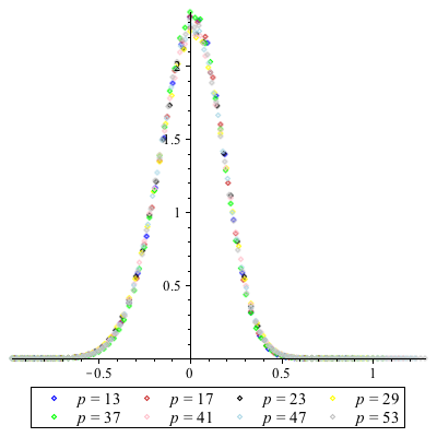
(a) Graph of $N^{\textrm{KS}}_{p,3}(\tau)$

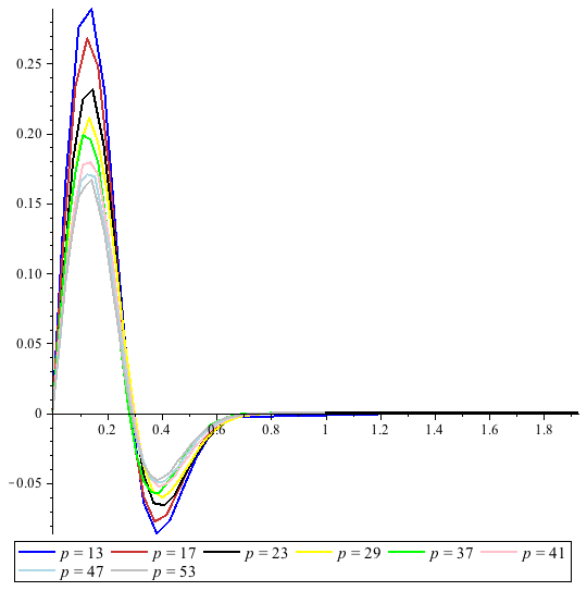
(b) Graph of $N^{\textrm{KS}}_{p,3}(\tau)-N^{\textrm{KS}}_{p,3}(-\tau)$

Figure 3. Trace distribution

References

- [1] D. Abramovich and F. Oort. Alterations and resolution of singularities. In Resolution of singularities (Obergurgl, 1997), volume 181 of Progr. Math., pages 39–108. Birkhäuser, Basel, 2000.
- [2] M. Artebani and S. Quispe. Fields of moduli and fields of definition of odd signature curves. Arch. Math., 99(4):333–344, 2012.
- [3] F. Bars. Automorphism groups of genus curves. Notes del seminari Corbes de Gèneres , 2006.
- [4] J. Bergström. Master’s thesis. PhD thesis, Kungl. Tekniska Högskolan, Stockholm, 2001.
- [5] J. Bergström. Cohomology of moduli spaces of curves of genus three via point counts. J. Reine Angew. Math., 622:155–187, 2008.
- [6] G. Cardona. On the number of curves of genus 2 over a finite field. Finite Fields Appl., 9(4):505–526, 2003.
- [7] J. Dixmier. On the projective invariants of quartic plane curves. Adv. in Math., 64:279–304, 1987.
- [8] I. V. Dolgachev. Classical algebraic geometry. Cambridge University Press, Cambridge, 2012. A modern view.
- [9] D. M. Freeman and T. Satoh. Constructing pairing-friendly hyperelliptic curves using Weil restriction. J. of Number Theory, 131(5):959–983, 2011.
- [10] M. Girard and D. R. Kohel. Classification of genus 3 curves in special strata of the moduli space. Hess, Florian (ed.) et al., Algorithmic number theory. 7th international symposium, ANTS-VII, Berlin, Germany, July 23–28, 2006. Proceedings. Berlin: Springer. Lecture Notes in Computer Science 4076, 346-360 (2006)., 2006.
- [11] S. P. Glasby and R. B. Howlett. Writing representations over minimal fields. Comm. Algebra, 25(6):1703–1711, 1997.
- [12] S. Gorchinskiy and F. Viviani. Picard group of moduli of hyperelliptic curves. Math. Z., 258(2):319–331, 2008.
- [13] B. H. Gross and J. Harris. On some geometric constructions related to theta characteristics. In Contributions to automorphic forms, geometry, and number theory, pages 279–311. Johns Hopkins Univ. Press, Baltimore, MD, 2004.
- [14] A. Guillevic and D. Vergnaud. Genus 2 hyperelliptic curve families with explicit jacobian order evaluation and pairing-friendly constructions. In Pairing-based cryptography—Pairing 2012, volume 7708 of Lecture Notes in Comput. Sci., pages 234–253. Springer, Berlin, 2012.
- [15] J. Harris and I. Morrison. Moduli of curves, volume 187 of Graduate Texts in Mathematics. Springer-Verlag, New York, 1998.
- [16] J. Harris and D. Mumford. On the Kodaira dimension of the moduli space of curves. Invent. Math., 67(1):23–88, 1982. With an appendix by William Fulton.
- [17] H.-W. Henn. Die Automorphismengruppen der algebraischen Funktionenkorper vom Geschlecht , 1976.
- [18] M. Homma. Automorphisms of prime order of curves. Manuscripta Math., 33(1):99–109 (1980).
- [19] E. W. Howe, K. E. Lauter, and J. Top. Pointless curves of genus three and four. In Algebra, Geometry, and Coding Theory (AGCT 2003) (Y. Aubry and G. Lachaud, eds.), volume 11 of Séminaires et Congrès. Société Mathématique de France, Paris, 2005.
- [20] B. Huggins. Fields of moduli and fields of definition of curves. PhD thesis, University of California, Berkeley, Berkeley, California, 2005. http://arxiv.org/abs/math.NT/0610247.
- [21] P. Katsylo. Rationality of the moduli variety of curves of genus 3. Comment. Math. Helv., 71(4):507–524, 1996.
- [22] N. M. Katz and P. Sarnak. Random matrices, Frobenius eigenvalues, and monodromy, volume 45 of American Mathematical Society Colloquium Publications. American Mathematical Society, Providence, RI, 1999.
- [23] R. Lercier and C. Ritzenthaler. Hyperelliptic curves and their invariants: geometric, arithmetic and algorithmic aspects. J. Algebra, 372:595–636, 2012.
- [24] R. Lercier, C. Ritzenthaler, and J. Sijsling. Fast computation of isomorphisms of hyperelliptic curves and explicit descent. In E. W. Howe and K. S. Kedlaya, editors, Proceedings of the Tenth Algorithmic Number Theory Symposium, pages 463–486. Mathematical Sciences Publishers, 2012.
- [25] K. Lønsted. The structure of some finite quotients and moduli for curves. Comm. Algebra, 8(14):1335–1370, 1980.
- [26] K. Magaard, T. Shaska, S. Shpectorov, and H. Völklein. The locus of curves with prescribed automorphism group. Communications in arithmetic fundamental groups (Kyoto, 1999/2001). Sūrikaisekikenkyūsho Kōkyūroku No. 1267 (2002), 112–141.
- [27] S. Meagher and J. Top. Twists of genus three curves over finite fields. Finite Fields Appl., 16(5):347–368, 2010.
- [28] P. E. Newstead. Introduction to moduli problems and orbit spaces, volume 51 of Tata Institute of Fundamental Research Lectures on Mathematics and Physics. Tata Institute of Fundamental Research, Bombay, 1978.
- [29] T. Ohno. The graded ring of invariants of ternary quartics I, 2005? unpublished.
- [30] C. Ritzenthaler. Point counting on genus 3 non hyperelliptic curves. In Algorithmic number theory, volume 3076 of Lecture Notes in Comput. Sci., pages 379–394. Springer, Berlin, 2004.
- [31] C. Ritzenthaler. Explicit computations of Serre’s obstruction for genus-3 curves and application to optimal curves. LMS J. Comput. Math., 13:192–207, 2010.
- [32] K. Rökaeus. Computer search for curves with many points among abelian covers of genus 2 curves. In Arithmetic, geometry, cryptography and coding theory, volume 574 of Contemp. Math., pages 145–150. Amer. Math. Soc., Providence, RI, 2012.
- [33] T. Satoh. Generating genus two hyperelliptic curves over large characteristic finite fields. In Advances in Cryptology: EUROCRYPT 2009, Cologne, volume 5479, Berlin, 2009. Springer.
- [34] T. Sekiguchi. Wild ramification of moduli spaces for curves or for abelian varieties. Compositio Math., 54:33–372, 1985.
- [35] J.-P. Serre. Corps locaux. Hermann, Paris, 1968. Deuxième édition, Publications de l’Université de Nancago, No. VIII.
- [36] T. Shioda. Plane quartics and Mordell-Weil lattices of type . Comment. Math. Univ. St. Paul., 42(1):61–79, 1993.
- [37] J. H. Silverman. The arithmetic of elliptic curves, volume 106 of Graduate Texts in Mathematics. Springer, Dordrecht, second edition, 2009.
- [38] Y. Varshavsky. On the characterization of complex Shimura varieties. Selecta Math. (N.S.), 8(2):283–314, 2002.
- [39] A. Vermeulen. Weierstrass points of weight two on curves of genus three. PhD thesis, university of Amsterdam, Amsterdam, 1983.
- [40] H. Weber. Theory of abelian functions of genus 3. (Theorie der Abel’schen Functionen vom Geschlecht 3.), 1876.
- [41] A. Weil. The field of definition of a variety. American Journal of Mathematics, 78:509–524, 1956.