Scaling instability of the buckling load in axially compressed circular cylindrical shells

Abstract

In this paper we initiate a program of rigorous analytical investigation of the paradoxical buckling behavior of circular cylindrical shells under axial compression. This is done by the development and systematic application of general theory of “near-flip” buckling of 3D slender bodies to cylindrical shells. The theory predicts scaling instability of the buckling load due to imperfections of load. It also suggests a more dramatic scaling instability caused by shape imperfections. The experimentally determined scaling exponent 1.5 of the critical stress as a function of shell thickness appears in our analysis as the scaling of the lower bound on safe loads given by the Korn constant. While the results of this paper fall short of a definitive explanation of the buckling behavior of cylindrical shells, we believe that our approach is capable of providing reliable estimates of the buckling loads of axially compressed cylindrical shells.

1 Introduction

A circular cylindrical shell loaded by an axial compressive stress will buckle producing a variety of buckling patterns[4, 20, 6], including the single-dimple buckle [32, 15], shown in Figure 1.

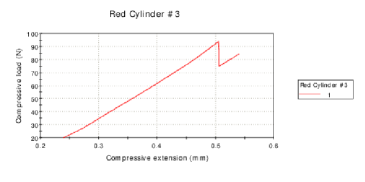
Figure 1: Single-dimple buckling pattern in buckled soda cans [14].

In the soda can experiments [14] this dimple consistently appeared with an audible click, corresponding to the drop in load in Figure 1 and disappears (also with a click) upon unloading. This suggests that the local material response is still linearly elastic, while the global non-linearity is purely geometric. The abrupt nature of the observed buckling suggests that the trivial branch, whose stress and strain are well-approximated by linear elasticity, becomes unstable with respect to the observed buckling variation.

The classical shell theory supplies the following formula for the critical stress [24, 27] (see also [28]):

$$\sigma_{\rm cr}=\frac{Eh}{\sqrt{3(1-\nu^{2})}},$$ (1.1)

where $E$ and $\nu$ are the Young modulus and the Poisson ratio, respectively, and $h=t/R$ is the ratio of the wall thickness to the radius of the cylinder. A large body of experimental results summarized in [20, 32] show that not only the theoretical value of the buckling load is about 4 to 5 times higher than the one observed in experiments, but the critical stress $\sigma_{\rm cr}$ scales like $h^{3/2}$ with $h$, in stark contradiction to (1.1). Such paradoxical behavior is generally attributed to the sensitivity of the buckling load to imperfections of load and shape [1, 26, 29, 10, 30], due to the subcritical nature of the bifurcation [18, 19, 23, 16] in the von-Kármán-Donnell equations. Yet, such an interpretation of the experimental results does not give a quantification of sensitivity to imperfections, and does little to explain the paradoxical $h^{1.5}$ scaling of the critical stress. These questions have been raised in [5, 32, 15], where a combination of heuristic arguments and numerical simulations were used to address the problem. In situations where the classical shell theory gives predictions inconsistent with experiment, one can question whether “sensitivity to imperfections” is the true source of the inconsistency, or whether the failure of the heuristic models to adequately describe stability of slender bodies is at play. In a companion paper [12] we give a rigorous proof of the asymptotical correctness of (1.1), showing that the second variation of the energy of the compressed shell, regarded as a 3D hyperelastic body, becomes negative when the load exceeds the critical value (1.1).

Recent years have seen significant progress in the rigorous analysis of dimensionally reduced theories of plates and shells based on $\Gamma$-convergence [8, 25, 9, 21, 22]. In this approach, one must postulate the scaling of energy and the forces a priori, whereby different scaling assumptions lead to different dimensionally reduced plate and shell equations. These analyses show that the tacit assumptions of validity of specific shell theories must be justified before conclusions about the elastic behavior of such shells can be regarded as rigorous. By contrast, the theory in [13], based on the study of second variation, has no need for such a priori assumptions, since it pursues a more modest goal of identifying a critical load at which the “trivial branch”, or “fundamental state”, of equilibria becomes weakly unstable. This exclusive targeting of the instability without any attempt to compute $\Gamma$-limiting models or capture a global bifurcation picture of post-buckling behavior leads to a significant simplification in the rigorous analysis of stability of slender structures. Most notably, our approach does not require compactness of arbitrary low energy sequences as in [8]. In particular, our method is applicable in situations where compactness fails, as is the case for the axially compressed cylindrical shells.

In this paper we prove that a constitutively reduced characterization of the buckling load, derived in [13], captures the buckling mode as well. A more convenient criterion for the validity of this characterization of buckling, derived in this paper, makes the theory applicable to a broader, compared to [13], class of slender structures, including axially compressed cylindrical shells. While our approach is capable of providing a rigorous proof of the classical formula (1.1) [12], it also reveals a possible mechanism of imperfection sensitivity that may explain the experimental results and their discrepancy with the classical theory. Specifically, we show that generic imperfections in loading will change the scaling law of $\sigma_{\rm cr}$ to $h^{5/4}$. Shape imperfections may lead to an even bigger jump in the scaling exponent of $\sigma_{\rm cr}$ from $h$ to $h^{3/2}$. The power law $h^{3/2}$ arises as the scaling of the Korn constant [11], shown to describe the universal lower bound on safe loads in [13]. This explanation of the experimentally observed scaling of the critical stress could be viewed as an improvement of the ingenuous but somewhat intuitive arguments in [5, 32].

Generically, shape imperfections eliminate sharp bifurcation transitions [2]. However, the abrupt appearance of the dimple-shaped buckle accompanied by an audible click in our experiments suggests that, in the case of a cylindrical shell, shape imperfections do not eliminate bifurcation instability. If this is indeed the case, our methods would be able to accurately predict the critical load and the corresponding buckling mode. However, the rigorous analysis of an imperfect cylindrical shell is beyond the scope of this paper, since all the estimates proved here and in our companion paper [11] are for the specific circular cylindrical shell geometry.

This paper is organized as follows. In Section 2 we extend the theory of buckling of general slender bodies based on the asymptotic analysis of second variation [13]. We define “compression tensor” and further develop the method of buckling equivalence [13]. Section 3 applies the theory in Section 2 and the asymptotics of the Korn and Korn-type constants proved in [11] to the computation of the scaling law of the buckling load. We next demonstrate scaling instabilities due to generic imperfections of load. We conclude the paper with a less rigorous discussion of imperfections of shape.

2 Buckling of slender structures

In this section we revisit the general theory of buckling developed in [13] in order to extend and apply it to buckling of axially compressed cylindrical shells. The theory provides a recipe for computing the asymptotics of buckling loads of slender structures, as the slenderness parameter goes to zero.

We follow the established tradition and use the energy criterion of stability. Namely, we say that the deformation $\bm{y}=\bm{y}(\bm{x})$, $\bm{x}\in\Omega\subset\mathbb{R}^{3}$ is stable if it is a weak local minimizer of the energy

$${\mathcal{E}}(\bm{y})=\int_{\Omega}W(\nabla\bm{y})d\bm{x}-\int_{\partial\Omega}\bm{y}\cdot\bm{t}(\bm{x})dS(\bm{x}),$$

where $W(\bm{F})$ is the energy density function of the body and $\bm{t}(\bm{x})$ is the vector of dead load tractions. The energy density $W(\bm{F})$ satisfies the four fundamental properties:

• Absence of prestress: $W_{\bm{F}}(\bm{I})=\bm{0}$;

• Frame indifference: $W(\bm{F}\bm{R})=W(\bm{F})$ for every $\bm{R}\in SO(3)$;

• Local stability of the trivial deformation $\bm{y}(\bm{x})=\bm{x}$: $(\mathsf{L}_{0}\bm{\xi},\bm{\xi})\geq 0$ for any $\bm{\xi}\in\mathbb{R}^{3\times 3}$, where $\mathsf{L}_{0}=W_{\bm{F}\bm{F}}(\bm{I})$ is the linearly elastic tensor of material properties;

• Non-degeneracy: $(\mathsf{L}_{0}\bm{\xi},\bm{\xi})=0$ if and only if $\bm{\xi}^{T}=-\bm{\xi}$.

Here, and elsewhere in this paper we use the notation $(\bm{A},\bm{B})=\mathrm{Tr}\,(\bm{A}\bm{B}^{T})$ for the Frobenius inner product on the space of $3\times 3$ matrices.

In [13] we attribute the universal nature of buckling to the two universal properties (P1) and (P2) of the energy density function because they guarantee non-convexity of $W(\bm{F})$ in any neighborhood of the identity $\bm{I}$. We also remark that properties (P3) and (P4) of $\mathsf{L}_{0}$ imply a uniform lower bound

$$(\mathsf{L}_{0}\bm{\xi},\bm{\xi})\geq\alpha_{\mathsf{L}_{0}}|\bm{\xi}_{\rm sym}|^{2},\qquad\bm{\xi}_{\rm sym}=\displaystyle\frac{1}{2}(\bm{\xi}+\bm{\xi}^{T})$$ (2.1)

for some $\alpha_{\mathsf{L}_{0}}>0$.

2.1 Trivial branch

Consider a sequence of progressively slender domains $\Omega_{h}$ parametrized by a dimensionless parameter $h$. For example, for circular cylindrical shells, $h$ is the ratio of cylinder wall thickness to the cylinder radius (we keep the ratio of cylinder height to its radius constant). We consider a loading program parametrized by the loading parameter $\lambda$ describing the magnitude of the applied tractions $\bm{t}(\bm{x};h,\lambda)=\lambda\bm{t}^{h}(\bm{x})+O(\lambda^{2})$, as $\lambda\to 0$, or as a measure of the prescribed strain. Here and below $O(\lambda^{\alpha})$ is understood uniformly in $\bm{x}\in\Omega_{h}$ and $h\in[0,h_{0}]$. Let $\bm{y}(\bm{x};h,\lambda)$ be a family of Lipschitz equilibria of

$${\mathcal{E}}(\bm{y};h,\lambda)=\int_{\Omega_{h}}W(\nabla\bm{y})d\bm{x}-\int_{\partial\Omega_{h}}\bm{y}(\bm{x})\cdot\bm{t}(\bm{x};h,\lambda)dS(\bm{x}).$$ (2.2)

defined on $\overline{\Omega}\times[0,h]\times[0,\lambda_{0}]$ for some $h_{0}>0$ and $\lambda_{0}>0$. The general theory can treat a wide range of boundary conditions. To describe one, we restrict $\bm{y}$ to an affine subspace of $W^{1,\infty}(\Omega_{h};\mathbb{R}^{3})$, given by

$$\bm{y}\in\overline{\bm{y}}(\bm{x};h,\lambda)+V_{h}^{\circ},$$ (2.3)

where $V_{h}^{\circ}$ is a linear subspace of $W^{1,\infty}(\Omega_{h};\mathbb{R}^{3})$ that contains $W_{0}^{1,\infty}(\Omega_{h};\mathbb{R}^{3})$ and does not depend on the loading parameter $\lambda$. The given function $\overline{\bm{y}}(\bm{x};h,\lambda)\in W^{1,\infty}(\Omega_{h};\mathbb{R}^{3})$ describes the “Dirichlet part” of the boundary conditions, while the traction vector $\bm{t}(\bm{x};h,\lambda)$ describes the Neumann-part. An example of such a description of the boundary conditions for the cylindrical shell will be given in Section 3.1.

Definition 2.1.

We call the family of Lipschitz equilibria $\bm{y}(\bm{x};h,\lambda)$ of ${\mathcal{E}}(\bm{y};h,\lambda)$ a linearly elastic trivial branch if there exist $h_{0}>0$ and $\lambda_{0}>0$, so that for every $h\in[0,h_{0}]$ and $\lambda\in[0,\lambda_{0}]$

• $\bm{y}(\bm{x};h,0)=\bm{x}$

• There exist a family of Lipschitz functions $\bm{u}^{h}(\bm{x})$, independent of $\lambda$, such that

  $$\|\nabla\bm{y}(\bm{x};h,\lambda)-\bm{I}-\lambda\nabla\bm{u}^{h}(\bm{x})\|_{L^{\infty}(\Omega_{h})}\leq C\lambda^{2},$$ (2.4)

• $$\|\displaystyle\frac{\partial(\nabla\bm{y})}{\partial\lambda}(\bm{x};h,\lambda)-\nabla\bm{u}^{h}(\bm{x})\|_{L^{\infty}(\Omega_{h})}\leq C\lambda$$ (2.5)

where the constant $C$ is independent of $h$ and $\lambda$.

We remark that neither uniqueness nor stability of the trivial branch are assumed.

The equilibrium equations and the boundary conditions satisfied by the trivial branch $\bm{y}(\bm{x};h,\lambda)$ can be written explicitly in the weak form:

$$\int_{\Omega_{h}}(W_{\bm{F}}(\nabla\bm{y}(\bm{x};h,\lambda)),\nabla\bm{\phi})d\bm{x}-\int_{\partial\Omega_{h}}\bm{\phi}\cdot\bm{t}(\bm{x};h,\lambda)dS=0,\qquad\bm{\phi}\in V_{h}^{\circ},$$ (2.6)

Differentiating (2.6) in $\lambda$ at $\lambda=0$, which is allowed due to (2.4), we obtain

$$\int_{\Omega_{h}}(\mathsf{L}_{0}\nabla\bm{u}^{h}(\bm{x}),\nabla\bm{\phi})d\bm{x}-\int_{\partial\Omega_{h}}\bm{\phi}\cdot\bm{t}^{h}(\bm{x})dS=0,\qquad\bm{\phi}\in V_{h}^{\circ},$$ (2.7)

In [13] the notion of the near-flip buckling is defined when for any $h\in[0,h_{0}]$ the trivial branch $\bm{y}(\bm{x};h,\lambda)$ becomes unstable for $\lambda>\lambda(h)$, where $\lambda(h)\to 0$, as $h\to 0$. This happens because it becomes energetically more advantageous to activate bending modes rather than store more compressive stress. This exchange of stability is detected by the change in sign of the second variation of energy

$$\delta^{2}{\mathcal{E}}(\bm{\phi};h,\lambda)=\int_{\Omega_{h}}(W_{\bm{F}\bm{F}}(\nabla\bm{y}(\bm{x};h,\lambda))\nabla\bm{\phi},\nabla\bm{\phi})d\bm{x},\qquad\bm{\phi}\in V_{h},$$

where $V_{h}=\overline{V_{h}^{\circ}}$ is the closure of $V_{h}^{\circ}$ in $W^{1,2}(\Omega_{h};\mathbb{R}^{3})$. The second variation is always non negative, when $0<\lambda<\lambda(h)$ and can become negative for some choice of the admissible variation $\bm{\phi}\in V_{h}$, when $\lambda>\lambda(h)$. It was understood in [13] that this failure of weak stability is due to properties (P1)–(P4) of $W(\bm{F})$ and is intimately related to flip instability in soft device.

2.2 Buckling load and buckling mode

Using the second variation criterion for stability we define the buckling load as

$$\lambda^{*}(h)=\inf\{\lambda>0:\delta^{2}{\mathcal{E}}(\bm{\phi};h,\lambda)<0\text{ for some }\bm{\phi}\in V_{h}\}.$$ (2.8)

Definition 2.2.

We say that the body undergoes a near-flip buckling if $\lambda^{*}(h)>0$ for all $h\in(0,h_{0})$, for some $h_{0}>0$, and $\lambda^{*}(h)\to 0$, as $h\to 0$.

We refer to [13] for a discussion of why this terminology is appropriate.

The buckling mode is generally understood as the variation $\bm{\phi}^{*}_{h}\in V_{h}\setminus\{0\}$, such that $\delta^{2}{\mathcal{E}}(\bm{\phi}^{*}_{h};h,\lambda^{*}(h))=0$. However, if we are only interested in the asymptotics of the critical load, as $h\to 0$, then we would not distinguish between $\lambda^{*}(h)$ and $\lambda(h)$, as long as $\lambda(h)/\lambda^{*}(h)\to 1$, as $h\to 0$. If we replace $\lambda^{*}(h)$ with $\lambda_{\epsilon}(h)=\lambda^{*}(h)(1+\epsilon)$, then we estimate

$$\delta^{2}{\mathcal{E}}(\bm{\phi}^{*}_{h};h,\lambda^{*}(h)(1+\epsilon))\approx\lambda^{*}(h)\epsilon\displaystyle\frac{\partial(\delta^{2}{\mathcal{E}})}{\partial\lambda}(\bm{\phi}^{*}_{h};h,\lambda^{*}(h)).$$

This means that for the purposes of asymptotics we should not distinguish differences in values of second variation that are infinitesimal, compared to

$$\lambda^{*}(h)\displaystyle\frac{\partial(\delta^{2}{\mathcal{E}})}{\partial\lambda}(\bm{\phi}^{*}_{h};h,\lambda^{*}(h)).$$

In keeping with these observations, we redefine the notion of the buckling load and buckling mode, under the assumption that the body undergoes a near-flip buckling in the sense of Definition 2.2.

Definition 2.3.

We say that $\lambda(h)\to 0$, as $h\to 0$ is a buckling load if

$$\lim_{h\to 0}\frac{\lambda(h)}{\lambda^{*}(h)}=1.$$ (2.9)

A buckling mode is a family of variations $\bm{\phi}_{h}\in V_{h}\setminus\{0\}$, such that

$$\lim_{h\to 0}\frac{\delta^{2}{\mathcal{E}}(\bm{\phi}_{h};h,\lambda^{*}(h))}{\lambda^{*}(h)\displaystyle\frac{\partial(\delta^{2}{\mathcal{E}})}{\partial\lambda}(\bm{\phi}_{h};h,\lambda^{*}(h))}=0.$$ (2.10)

The most important insight in [13] is that at the critical load $\lambda^{*}(h)\to 0$, as $h\to 0$, the local material response is well inside the linearly elastic regime and the instability can be detected by a simpler constitutively linearized second variation:

$$\delta^{2}{\mathcal{E}}_{cl}(\bm{\phi};h,\lambda)=\int_{\Omega_{h}}\{(\mathsf{L}_{0}e(\bm{\phi}),e(\bm{\phi}))+\lambda(\bm{\sigma}_{h},\nabla\bm{\phi}^{T}\nabla\bm{\phi})\}d\bm{x},\qquad\bm{\phi}\in V_{h}$$ (2.11)

where $e(\bm{\phi})=\displaystyle\frac{1}{2}(\nabla\bm{\phi}+(\nabla\bm{\phi})^{T})$ and

$$\bm{\sigma}_{h}(\bm{x})=\mathsf{L}_{0}e(\bm{u}^{h}(\bm{x}))$$ (2.12)

is the linear elastic stress. We define

$$\mathfrak{C}_{h}(\bm{\phi})=\displaystyle\frac{\partial(\delta^{2}{\mathcal{E}}_{cl})}{\partial\lambda}(\bm{\phi};h,\lambda)=\int_{\Omega_{h}}(\bm{\sigma}_{h},\nabla\bm{\phi}^{T}\nabla\bm{\phi})d\bm{x}.$$ (2.13)

Observe that

$${\mathcal{A}}_{h}=\left\{\bm{\phi}\in V_{h}:\mathfrak{C}_{h}(\bm{\phi})<0\right\}$$ (2.14)

can be regarded as the set of all destabilizing variations for (2.11). We assume that the applied loading has a compressive nature. In particular, we assume that the sets ${\mathcal{A}}_{h}$ are non-empty for all $h\in(0,h_{0})$ for some $h_{0}>0$. In parallel with our discussion of the asymptotics of the critical load and buckling mode we define the functional

$$\mathfrak{R}(h,\bm{\phi})=-\frac{\int_{\Omega_{h}}(\mathsf{L}_{0}e(\bm{\phi}),e(\bm{\phi}))d\bm{x}}{\int_{\Omega_{h}}(\bm{\sigma}_{h},\nabla\bm{\phi}^{T}\nabla\bm{\phi})d\bm{x}}=-\frac{\mathfrak{S}_{h}(\bm{\phi})}{\mathfrak{C}_{h}(\bm{\phi})},$$ (2.15)

where

$$\mathfrak{S}_{h}(\bm{\phi})=\int_{\Omega_{h}}(\mathsf{L}_{0}e(\bm{\phi}),e(\bm{\phi}))d\bm{x}.$$ (2.16)

is the measure of stability of the trivial branch. The constitutively linearized buckling load and buckling mode are then defined by analogy with the original second variation.

Definition 2.4.

The constitutively linearized buckling load $\widehat{\lambda}(h)$ is defined by

$$\widehat{\lambda}(h)=\inf_{\bm{\phi}\in{\mathcal{A}}_{h}}\mathfrak{R}(h,\bm{\phi}).$$ (2.17)

We say that the family of variations $\{\bm{\phi}_{h}\in{\mathcal{A}}_{h}:h\in(0,h_{0})\}$ is a constitutively linearized buckling mode if

$$\lim_{h\to 0}\frac{\mathfrak{R}(h,\bm{\phi}_{h})}{\widehat{\lambda}(h)}=1.$$ (2.18)

We now need to prove that under some reasonable assumptions the constitutively linearized buckling load and buckling mode are buckling mode and buckling mode, respectively, in the sense of Definition 2.3.

Recall the definition of the Korn constant

$$K(V_{h})=\inf_{\bm{\phi}\in V_{h}}\frac{\|e(\bm{\phi})\|^{2}}{\|\nabla\bm{\phi}\|^{2}}.$$ (2.19)

Here and elsewhere in this paper $\|\cdot\|$ always denotes the $L^{2}$-norm on $\Omega_{h}$.

Definition 2.5.

We say that the body $\Omega_{h}$ is slender if

$$\lim_{h\to 0}K(V_{h})=0.$$ (2.20)

We remark that this notion of slenderness, introduced in [13], is not purely geometric, but depends on the type of loading described by the subspace $V_{h}$. On the one hand, a thin rod or a plate in the hard device will not be regarded as slender, since their Korn constant is 1/2, regardless of their geometric slenderness. On the other hand, a geometrically non-slender body, such as a ball or a cube will not be slender under our definition, for any boundary conditions that exclude all rigid body motions.

Theorem 2.6 (Asymptotics of the critical load).

Suppose that the body is slender in the sense of Definition 2.5. Assume that the constitutively linearized critical load $\widehat{\lambda}(h)$, defined in (2.17) satisfies $\widehat{\lambda}(h)>0$ for all sufficiently small $h$ and

$$\lim_{h\to 0}\frac{\widehat{\lambda}(h)^{2}}{K(V_{h})}=0.$$ (2.21)

Then $\widehat{\lambda}(h)$ is the buckling load and any constitutively linearized buckling mode $\bm{\phi}_{h}$ is a buckling mode in the sense of Definition 2.3.

The theorem is proved by means of the basic estimate, which is a simple modification of the estimates in [13] used in the derivation of the formula for $\delta^{2}{\mathcal{E}}_{cl}(\bm{\phi};h,\lambda)$:

Lemma 2.7.

Suppose $\bm{y}(\bm{x};h,\lambda)$ satisfies (2.4) and $W(\bm{F})$ has the properties (P1)–(P4). Then

$$\left|\delta^{2}{\mathcal{E}}(\bm{\phi};h,\lambda)-\delta^{2}{\mathcal{E}}_{cl}(\bm{\phi};h,\lambda)\right|\leq C\left(\frac{\lambda}{\sqrt{K(V_{h})}}+\frac{\lambda^{2}}{K(V_{h})}\right)\mathfrak{S}_{h}(\bm{\phi}).$$ (2.22)

and

$$\left|\displaystyle\frac{\partial(\delta^{2}{\mathcal{E}})}{\partial\lambda}(\bm{\phi};h,\lambda)-\mathfrak{C}_{h}(\bm{\phi})\right|\leq C\left(\frac{1}{\sqrt{K(V_{h})}}+\frac{\lambda}{K(V_{h})}\right)\mathfrak{S}_{h}(\bm{\phi}).$$ (2.23)

where the constant $C$ is independent of $h$, $\lambda$ and $\bm{\phi}$.

Proof.

According to the frame indifference property (P2), $W(\bm{F})=\widehat{W}(\bm{F}^{T}\bm{F})$. Differentiating this formula twice we obtain

$$(W_{\bm{F}\bm{F}}(\bm{F})\bm{\xi},\bm{\xi})=4(\widehat{W}_{\bm{C}\bm{C}}(\bm{C})(\bm{F}^{T}\bm{\xi}),\bm{F}^{T}\bm{\xi})+2(\widehat{W}_{\bm{C}}(\bm{C}),\bm{\xi}^{T}\bm{\xi}),\qquad\bm{C}=\bm{F}^{T}\bm{F}.$$ (2.24)

We can estimate

$$|(\widehat{W}_{\bm{C}\bm{C}}(\bm{C})(\bm{F}^{T}\bm{\xi}),\bm{F}^{T}\bm{\xi})-(\widehat{W}_{\bm{C}\bm{C}}(\bm{I})\bm{\xi},\bm{\xi})|\leq|(\widehat{W}_{\bm{C}\bm{C}}(\bm{C})(\bm{F}^{T}-\bm{I})\bm{\xi},(\bm{F}^{T}-\bm{I})\bm{\xi})|+$$

$$|((\widehat{W}_{\bm{C}\bm{C}}(\bm{C})-\widehat{W}_{\bm{C}\bm{C}}(\bm{I}))\bm{\xi},\bm{\xi})|+2|(\widehat{W}_{\bm{C}\bm{C}}(\bm{C})\bm{\xi},(\bm{F}^{T}-\bm{I})\bm{\xi})|$$

When $\bm{F}$ is uniformly bounded we obtain

$$|(\widehat{W}_{\bm{C}\bm{C}}(\bm{C})(\bm{F}^{T}\bm{\xi}),\bm{F}^{T}\bm{\xi})-(\widehat{W}_{\bm{C}\bm{C}}(\bm{I})\bm{\xi},\bm{\xi})|\leq C\left(|\bm{F}-\bm{I}|^{2}|\bm{\xi}|^{2}+|\bm{C}-\bm{I}||\bm{\xi}_{\rm sym}|^{2}+|\bm{F}-\bm{I}||\bm{\xi}_{\rm sym}||\bm{\xi}|\right).$$

Similarly,

$$|(\widehat{W}_{\bm{C}}(\bm{C})-\widehat{W}_{\bm{C}\bm{C}}(\bm{I})(\bm{C}-\bm{I}),\bm{\xi}^{T}\bm{\xi})|\leq C|\bm{C}-\bm{I}|^{2}|\bm{\xi}|^{2}$$

When $\bm{F}=\nabla\bm{y}(\bm{x};h,\lambda)$ and $\bm{\xi}=\nabla\bm{\phi}$ we obtain, taking into account (2.4), that

$$|\bm{F}-\bm{I}|\leq C\lambda,\qquad|\bm{C}-\bm{I}|\leq C\lambda.$$

Observing that

$$4\widehat{W}_{\bm{C}\bm{C}}(\bm{I})=W_{\bm{F}\bm{F}}(\bm{I})=\mathsf{L}_{0},\qquad|\bm{C}-\bm{I}-2\lambda e(\bm{u}^{h})|\leq C\lambda^{2}.$$

we obtain the estimate

$$|(W_{\bm{F}\bm{F}}(\bm{F})\bm{\xi},\bm{\xi})-(\mathsf{L}_{0}\bm{\xi}_{\rm sym},\bm{\xi}_{\rm sym})-\lambda(\bm{\sigma}_{h},\bm{\xi}^{T}\bm{\xi})|\leq C(\lambda|\bm{\xi}_{\rm sym}||\bm{\xi}|+\lambda^{2}|\bm{\xi}|^{2}).$$

Integrating over $\Omega_{h}$ as using the coercivity (2.1) of $\mathsf{L}_{0}$ we obtain the estimate (2.22).

In order to prove the estimate (2.23) we substitute $\bm{F}=\nabla\bm{y}(\bm{x};h,\lambda)$ and $\bm{\xi}=\nabla\bm{\phi}$ into (2.24) and differentiate in $\lambda$, obtaining

$$\frac{\partial(W_{\bm{F}\bm{F}}(\bm{F})\bm{\xi},\bm{\xi})}{\partial\lambda}=4((\widehat{W}_{\bm{C}\bm{C}\bm{C}}(\bm{C})\dot{\bm{C}})(\bm{F}^{T}\bm{\xi}),\bm{F}^{T}\bm{\xi})+8(\widehat{W}_{\bm{C}\bm{C}}(\bm{C})(\bm{F}^{T}\bm{\xi}),\dot{\bm{F}}^{T}\bm{\xi})+2(\widehat{W}_{\bm{C}\bm{C}}(\bm{C})\dot{\bm{C}},\bm{\xi}^{T}\bm{\xi}),$$

where $\dot{\bm{C}}$ and $\dot{\bm{F}}$ denote differentiation with respect to $\lambda$. Using the uniform boundedness of $\dot{\bm{C}}$, which is a corollary of (2.5), as well as (2.4) we estimate

$$|((\widehat{W}_{\bm{C}\bm{C}\bm{C}}(\bm{C})\dot{\bm{C}})(\bm{F}^{T}\bm{\xi}),\bm{F}^{T}\bm{\xi})|\leq C(|\bm{\xi}_{\rm sym}|^{2}+\lambda|\bm{\xi}||\bm{\xi}_{\rm sym}|).$$

and

$$|(\widehat{W}_{\bm{C}\bm{C}}(\bm{C})(\bm{F}^{T}\bm{\xi}),\dot{\bm{F}}^{T}\bm{\xi})|\leq C(|\bm{\xi}||\bm{\xi}_{\rm sym}|+\lambda|\bm{\xi}|^{2}).$$

We also estimate, using $|\bm{C}-\bm{I}|\leq C\lambda$ and $|\dot{\bm{C}}-2e(\bm{u}^{h})|\leq C\lambda$, that are consequences of (2.4) and (2.5):

$$|2(\widehat{W}_{\bm{C}\bm{C}}(\bm{C})\dot{\bm{C}},\bm{\xi}^{T}\bm{\xi})-(\bm{\sigma}_{h},\bm{\xi}^{T}\bm{\xi})|\leq C\lambda|\bm{\xi}|^{2}.$$

∎

Proof of Theorem 2.6.

By definition of $\widehat{\lambda}(h)$, for any $\epsilon>0$ and any $h\in(0,h_{0})$ there exists $\bm{\phi}_{h}\in{\mathcal{A}}_{h}$ such that

$$\mathfrak{S}_{h}(\bm{\phi}_{h})+\widehat{\lambda}(h)(1+\epsilon)\mathfrak{C}_{h}(\bm{\phi}_{h})<0,$$ (2.25)

thus,

$$\delta^{2}{\mathcal{E}}_{cl}(\bm{\phi}_{h};h,\widehat{\lambda}(h)(1+2\epsilon))\leq-\frac{\epsilon\mathfrak{S}_{h}(\bm{\phi}_{h})}{1+\epsilon}.$$

The estimate (2.22) gives the upper bound on the second variation:

$$\delta^{2}{\mathcal{E}}(\bm{\phi}_{h};h,\widehat{\lambda}(h)(1+2\epsilon))\leq\left(-\frac{\epsilon}{(1+\epsilon)}+C\left(\frac{\widehat{\lambda}(h)}{\sqrt{K(V_{h})}}+\frac{\widehat{\lambda}(h)^{2}}{K(V_{h})}\right)\right)\mathfrak{S}_{h}(\bm{\phi}_{h}),$$

Thus, due to (2.21), for sufficiently small $h$, we have $\delta^{2}{\mathcal{E}}(\bm{\phi}_{h};h,\widehat{\lambda}(h)(1+2\epsilon))<0$, and hence $\lambda^{*}(h)\leq\widehat{\lambda}(h)(1+2\epsilon)$. We conclude that

$$\mathop{\overline{\lim}}_{h\to 0}\frac{\lambda^{*}(h)}{\widehat{\lambda}(h)}\leq 1.$$ (2.26)

To prove the opposite inequality we observe that by definition of $\widehat{\lambda}(h)$ we have

$$\mathfrak{S}_{h}(\bm{\phi})+\widehat{\lambda}(h)\mathfrak{C}_{h}(\bm{\phi})\geq 0$$

for any $\bm{\phi}\in V_{h}$. Therefore, for any $\epsilon>0$ and any $0<\lambda\leq\widehat{\lambda}(h)(1-\epsilon))$ we have

$$\delta^{2}{\mathcal{E}}_{cl}(\bm{\phi};h,\lambda)\geq\epsilon\mathfrak{S}_{h}(\bm{\phi}).$$

The estimate (2.22) now gives the lower bound on the second variation:

$$\delta^{2}{\mathcal{E}}(\bm{\phi};h,\lambda)\geq\left(\epsilon-C\left(\frac{\widehat{\lambda}(h)}{\sqrt{K(V_{h})}}+\frac{\widehat{\lambda}(h)^{2}}{K(V_{h})}\right)\right)\mathfrak{S}_{h}(\bm{\phi}),$$

Thus for all sufficiently small $h$ and all $\bm{\phi}\in V_{h}\setminus\{0\}$ we have $\delta^{2}{\mathcal{E}}(\bm{\phi};h,\lambda)>0$ for all $0<\lambda\leq\widehat{\lambda}(h)(1-\epsilon)$, which means that $\lambda^{*}(h)\geq\widehat{\lambda}(h)(1-\epsilon)$. This implies

$$\mathop{\underline{\lim}}_{h\to 0}\frac{\lambda^{*}(h)}{\widehat{\lambda}(h)}\geq 1.$$ (2.27)

Combining (2.26) and (2.27) we conclude that $\widehat{\lambda}(h)$ is the buckling load.

Assume now that $\bm{\phi}_{h}$ is a constitutively linearized buckling mode, i.e. (2.18) holds. Set $\lambda=\lambda^{*}(h)$ and $\bm{\phi}=\bm{\phi}_{h}$ in the inequality (2.22). Then, dividing both sides of the inequality by $-\lambda^{*}(h)\mathfrak{C}_{h}(\bm{\phi}_{h})>0$ we obtain

$$\left|\frac{\delta^{2}{\mathcal{E}}(\bm{\phi}_{h};h,\lambda^{*}(h))}{-\lambda^{*}(h)\mathfrak{C}_{h}(\bm{\phi}_{h})}-\left(\frac{\mathfrak{R}(h,\bm{\phi}_{h})}{\lambda^{*}(h)}-1\right)\right|\leq C\left(\frac{\lambda^{*}(h)}{\sqrt{K(V_{h})}}+\frac{(\lambda^{*}(h))^{2}}{K(V_{h})}\right)\frac{\mathfrak{R}(h,\bm{\phi}_{h})}{\lambda^{*}(h)}.$$

Since we have proved that $\widehat{\lambda}(h)$ is the buckling load we conclude that

$$\lim_{h\to 0}\frac{\delta^{2}{\mathcal{E}}(\bm{\phi}_{h};h,\lambda^{*}(h))}{\lambda^{*}(h)\mathfrak{C}_{h}(\bm{\phi}_{h})}=0.$$

Similarly, setting $\lambda=\lambda^{*}(h)$ and $\bm{\phi}=\bm{\phi}_{h}$ in the inequality (2.23) and dividing both sides of the inequality by $-\mathfrak{C}_{h}(\bm{\phi}_{h})>0$ we obtain

$$\left|\frac{\displaystyle\frac{\partial(\delta^{2}{\mathcal{E}})}{\partial\lambda}(\bm{\phi}_{h};h,\lambda^{*}(h))}{-\mathfrak{C}_{h}(\bm{\phi}_{h})}+1\right|\leq C\left(\frac{\lambda^{*}(h)}{\sqrt{K(V_{h})}}+\frac{(\lambda^{*}(h))^{2}}{K(V_{h})}\right)\frac{\mathfrak{R}(h,\bm{\phi}_{h})}{\lambda^{*}(h)}.$$

We conclude that

$$\lim_{h\to 0}\frac{\displaystyle\frac{\partial(\delta^{2}{\mathcal{E}})}{\partial\lambda}(\bm{\phi}_{h};h,\lambda^{*}(h))}{\mathfrak{C}_{h}(\bm{\phi}_{h})}=1.$$

It follows now that $\bm{\phi}_{h}$ satisfies (2.10), and the theorem is proved. ∎

An immediate consequence of our Rayleigh quotient characterization of buckling load (2.17) is the safe load estimate:

$$\widehat{\lambda}(h)=\inf_{\bm{\phi}\in{\mathcal{A}}_{h}}\mathfrak{R}(h,\bm{\phi})\geq\inf_{\bm{\phi}\in V_{h}}\frac{\mathfrak{S}_{h}(\bm{\phi})}{\|\bm{\sigma}_{h}\|_{\infty}\|\nabla\bm{\phi}\|^{2}}=\frac{K_{\mathsf{L}_{0}}(V_{h})}{\|\bm{\sigma}_{h}\|_{\infty}},$$

where

$$K_{\mathsf{L}_{0}}(V_{h})=\inf_{\bm{\phi}\in V_{h}}\frac{\int_{\Omega_{h}}(\mathsf{L}_{0}e(\bm{\phi}),e(\bm{\phi}))d\bm{x}}{\|\nabla\bm{\phi}\|^{2}}.$$

We remark that rods and plates have buckling loads proportional to $K_{\mathsf{L}_{0}}(V_{h})$, while the theoretical buckling load for axially compressed circular cylindrical shells is much higher. Based on this, we conjecture that buckling loads that scale with $K(V_{h})$ should not exhibit sensitivity to imperfections.

2.3 Buckling equivalence

In the previous subsection we showed that the asymptotics of the critical load and buckling mode can be captured by a constitutively linearized functional $\mathfrak{R}(h,\bm{\phi})$. Even though such a characterization of buckling represents a significant simplification, compared to the characterization based on the second variation of a fully non-linear energy functional, further simplifications may be necessary to obtain explicit analytic expressions in specific problems. We envision two ways in which the analysis of buckling can be simplified. One is the simplification of the functional $\mathfrak{R}(h,\bm{\phi})$. The other is replacing the space of all admissible functions ${\mathcal{A}}_{h}$ with a smaller space ${\mathcal{B}}_{h}$. For example, we may want to use a specific ansatz, like the Kirchhoff ansatz in buckling of rods and plates. In order to formalize our simplification procedure we make the following definitions.

Definition 2.8.

Assume that $J(h,\bm{\phi})$ is a variational functional defined on ${\mathcal{B}}_{h}\subset{\mathcal{A}}_{h}$. We say that the pair $({\mathcal{B}}_{h},J(h,\bm{\phi}))$ characterizes buckling if the following three conditions are satisfied

1. Characterization of the buckling load: If

   $$\lambda(h)=\inf_{\bm{\phi}\in{\mathcal{B}}_{h}}J(h,\bm{\phi}),$$

   then $\lambda(h)$ is a buckling load in the sense of Definition 2.3.

2. Characterization of the buckling mode: If $\bm{\phi}_{h}\in{\mathcal{B}}_{h}$ is a buckling mode in the sense of Definition 2.3, then

   $$\lim_{h\to 0}\frac{J(h,\bm{\phi}_{h})}{\lambda(h)}=1.$$ (2.28)

3. Faithful representation of the buckling mode: If $\bm{\phi}_{h}\in{\mathcal{B}}_{h}$ satisfies (2.28) then it is a buckling mode.

Definition 2.9.

Two pairs $({\mathcal{B}}_{h},J_{1}(h,\bm{\phi}))$ and $({\mathcal{C}}_{h},J_{2}(h,\bm{\phi}))$ are called buckling equivalent if the pair $({\mathcal{B}}_{h},J_{1}(h,\bm{\phi}))$ characterizes buckling if and only if $({\mathcal{C}}_{h},J_{2}(h,\bm{\phi}))$ does.

The notion of buckling equivalence of functionals $({\mathcal{B}}_{h},J(h,\bm{\phi}))$ is an extension of B-equivalence, introduced in [13], in that it also captures buckling modes in addition to buckling loads.

Let us first address a simple question of restricting the space of functions ${\mathcal{B}}_{h}$ to an “ansatz” ${\mathcal{C}}_{h}$.

Lemma 2.10.

Suppose the pair $({\mathcal{B}}_{h},J(h,\bm{\phi}))$ characterizes buckling. Let ${\mathcal{C}}_{h}\subset{\mathcal{B}}_{h}$ be such that it contains a buckling mode. Then the pair $({\mathcal{C}}_{h},J(h,\bm{\phi}))$ characterizes buckling.

Proof.

Let

$$\lambda(h)=\inf_{\bm{\phi}\in{\mathcal{B}}_{h}}J(h,\bm{\phi}),\qquad\widetilde{\lambda}(h)=\inf_{\bm{\phi}\in{\mathcal{C}}_{h}}J(h,\bm{\phi}).$$

Then, clearly, $\widetilde{\lambda}(h)\geq\lambda(h)$. By assumption there exists a buckling mode $\bm{\phi}_{h}\in{\mathcal{C}}_{h}\subset{\mathcal{B}}_{h}$. Therefore,

$$\mathop{\overline{\lim}}_{h\to 0}\frac{\widetilde{\lambda}(h)}{\lambda(h)}\leq\lim_{h\to 0}\frac{J(h,\bm{\phi}_{h})}{\lambda(h)}=1,$$

since the pair $({\mathcal{B}}_{h},J(h,\bm{\phi}))$ characterizes buckling. Hence

$$\lim_{h\to 0}\frac{\widetilde{\lambda}(h)}{\lambda(h)}=1,$$ (2.29)

and part (a) of Definition 2.8 is established.

If $\bm{\phi}_{h}\in{\mathcal{C}}_{h}\subset{\mathcal{B}}_{h}$ is a buckling mode then

$$\lim_{h\to 0}\frac{J(h,\bm{\phi}_{h})}{\lambda(h)}=1,$$

since the pair $({\mathcal{B}}_{h},J(h,\bm{\phi}))$ characterizes buckling. Part (b) now follows from (2.29).

Finally, if $\bm{\phi}_{h}\in{\mathcal{C}}_{h}$ satisfies

$$\lim_{h\to 0}\frac{J(h,\bm{\phi}_{h})}{\widetilde{\lambda}(h)}=1,$$

then, $\bm{\phi}_{h}\in{\mathcal{B}}_{h}$ and by (2.29) we also have

$$\lim_{h\to 0}\frac{J(h,\bm{\phi}_{h})}{\lambda(h)}=1.$$

Therefore, $\bm{\phi}_{h}$ is a buckling mode. The Lemma is proved now. ∎

Our key tool for simplification of the functionals $J(h,\bm{\phi})$ characterizing buckling is the following theorem.

Theorem 2.11 (Buckling equivalence).

Suppose that $\lambda(h)$ is a buckling load in the sense of Definition 2.3. If either

$$\lim_{h\to 0}\lambda(h)\sup_{\bm{\phi}\in{\mathcal{B}}_{h}}\left|\frac{1}{J_{1}(h,\bm{\phi})}-\frac{1}{J_{2}(h,\bm{\phi})}\right|=0,$$ (2.30)

or

$$\lim_{h\to 0}\displaystyle\frac{1}{\lambda(h)}\sup_{\bm{\phi}\in{\mathcal{B}}_{h}}|J_{1}(h,\bm{\phi})-J_{2}(h,\bm{\phi})|=0,$$ (2.31)

then the pairs $({\mathcal{B}}_{h},J_{1}(h,\bm{\phi}))$ and $({\mathcal{B}}_{h},J_{2}(h,\bm{\phi}))$ are buckling equivalent in the sense of Definition 2.9.

Proof.

Let us introduce the following notation:

$$\lambda_{i}(h)=\inf_{\bm{\phi}\in{\mathcal{B}}_{h}}J_{i}(h,\bm{\phi}),\quad i=1,2.$$

$$\delta_{1}(h)=\lambda(h)\sup_{\bm{\phi}\in{\mathcal{B}}_{h}}\left|\frac{1}{J_{1}(h,\bm{\phi})}-\frac{1}{J_{2}(h,\bm{\phi})}\right|.$$

$$\delta_{2}(h)=\displaystyle\frac{1}{\lambda(h)}\sup_{\bm{\phi}\in{\mathcal{B}}_{h}}|J_{1}(h,\bm{\phi})-J_{2}(h,\bm{\phi})|.$$

Then

$$\left|\frac{\lambda(h)}{\lambda_{1}(h)}-\frac{\lambda(h)}{\lambda_{2}(h)}\right|=\lambda(h)\left|\sup_{\bm{\phi}\in{\mathcal{B}}_{h}}\frac{1}{J_{1}(h,\bm{\phi})}-\sup_{\bm{\phi}\in{\mathcal{B}}_{h}}\frac{1}{J_{2}(h,\bm{\phi})}\right|\leq\delta_{1}(h)$$

and

$$\frac{|\lambda_{1}(h)-\lambda_{2}(h)|}{\lambda(h)}=\displaystyle\frac{1}{\lambda(h)}\left|\inf_{\bm{\phi}\in{\mathcal{B}}_{h}}J_{1}(h,\bm{\phi})-\inf_{\bm{\phi}\in{\mathcal{B}}_{h}}J_{2}(h,\bm{\phi})\right|\leq\delta_{2}(h)$$

Assume that $({\mathcal{B}}_{h},J_{1}(h,\bm{\phi}))$ characterizes buckling. Then we have just proved that if either $\delta_{1}(h)\to 0$ or $\delta_{2}(h)\to 0$, as $h\to 0$, then $\lambda_{2}(h)/\lambda(h)\to 1$, as $h\to 0$, and condition (a) in Definition 2.8 is proved for $J_{2}(h,\bm{\phi})$.

Observe that by parts (b) and (c) of Definition 2.8 $\bm{\phi}_{h}\in{\mathcal{B}}_{h}$ is the buckling mode if and only if

$$\lim_{h\to 0}\frac{J_{1}(h,\bm{\phi}_{h})}{\lambda_{1}(h)}=1.$$

This is equivalent to

$$\lim_{h\to 0}\frac{\lambda(h)}{J_{1}(h,\bm{\phi}_{h})}=1.$$

Therefore,

$$\lim_{h\to 0}\frac{J_{2}(h,\bm{\phi}_{h})}{\lambda(h)}=1,$$

since either

$$\left|\frac{\lambda(h)}{J_{1}(h,\bm{\phi}_{h})}-\frac{\lambda(h)}{J_{2}(h,\bm{\phi}_{h})}\right|\leq\delta_{1}(h)$$

or

$$\frac{|J_{1}(h,\bm{\phi}_{h})-J_{2}(h,\bm{\phi}_{h})|}{\lambda(h)}\leq\delta_{2}(h)$$

Thus, in view of part (a), $\bm{\phi}_{h}$ is a buckling mode if and only if

$$\lim_{h\to 0}\frac{J_{2}(h,\bm{\phi}_{h})}{\lambda_{2}(h)}=1.$$

∎

As an application of Theorem 2.11 we show that we can simplify the Rayleigh quotient $\mathfrak{R}(h,\bm{\phi})$ further.

Theorem 2.12.

Suppose that the critical load $\widehat{\lambda}(h)$ satisfies (2.21). Let

$$\mathfrak{R}_{0}(h,\bm{\phi})=-\frac{\int_{\Omega_{h}}(\mathsf{L}_{0}e(\bm{\phi}),e(\bm{\phi}))d\bm{x}}{\displaystyle\frac{1}{4}\int_{\Omega_{h}}(\widetilde{\bm{\sigma}}_{h}\nabla\times\bm{\phi},\nabla\times\bm{\phi})d\bm{x}}=-\frac{\mathfrak{S}_{h}(\bm{\phi})}{\mathfrak{C}_{h}^{0}(\bm{\phi})},$$

where

$$\widetilde{\bm{\sigma}}_{h}=(\mathrm{Tr}\,\bm{\sigma}_{h})\bm{I}-\bm{\sigma}_{h}$$ (2.32)

is the compression tensor. Then $({\mathcal{A}}_{h},\mathfrak{R}(h,\bm{\phi}))$ and $({\mathcal{A}}_{h},\mathfrak{R}_{0}(h,\bm{\phi}))$ are buckling equivalent.

Proof.

For $\bm{a}\in\mathbb{R}^{3}$, let $\pi(\bm{a})$ denote a $3\times 3$ antisymmetric matrix defined by the cross-product map:

$$\pi(\bm{a})\bm{u}=\bm{a}\times\bm{u}.$$

Then $\nabla\bm{\phi}-(\nabla\bm{\phi})^{T}=\pi(\nabla\times\bm{\phi})$. We observe that replacing $\nabla\bm{\phi}$ with $e(\bm{\phi})-\pi(\nabla\times\bm{\phi})/2$ in $\mathfrak{C}_{h}(\bm{\phi})$ we obtain

$$\mathfrak{C}_{h}(\bm{\phi})=\int_{\Omega_{h}}\left(\bm{\sigma}_{h},e(\bm{\phi})^{2}+e(\bm{\phi})\pi(\nabla\times\bm{\phi})\right)d\bm{x}+\mathfrak{C}^{0}_{h}(\bm{\phi}).$$

It follows that for every $\bm{\phi}\in V_{h}$

$$|\mathfrak{C}_{h}(\bm{\phi})-\mathfrak{C}^{0}_{h}(\bm{\phi})|\leq\|\bm{\sigma}_{h}\|_{\infty}(\|e(\bm{\phi})\|^{2}+2\|e(\bm{\phi})\|\|\nabla\bm{\phi}\|)\leq\|\bm{\sigma}_{h}\|_{\infty}\|e(\bm{\phi})\|^{2}\left(1+\frac{2}{\sqrt{K(V_{h})}}\right).$$

Recalling that, due to (2.1),

$$\mathfrak{S}_{h}(\bm{\phi})\geq\alpha_{\mathsf{L}_{0}}\|e(\bm{\phi})\|^{2}$$

we obtain

$$\widehat{\lambda}(h)\left|\displaystyle\frac{1}{\mathfrak{R}(h,\bm{\phi})}-\displaystyle\frac{1}{\mathfrak{R}_{0}(h,\bm{\phi}))}\right|\leq\frac{\|\bm{\sigma}_{h}\|_{\infty}}{\alpha_{\mathsf{L}_{0}}}\left(\widehat{\lambda}(h)+\frac{2\widehat{\lambda}(h)}{\sqrt{K(V_{h})}}\right).$$

Thus (2.21) implies that the sufficient condition (2.30) for buckling equivalence is satisfied. The theorem is proved. ∎

We remark that $\nabla\times\bm{\phi}$ is a scalar in 2D, and similar calculations show that the functional $\mathfrak{R}(h,\bm{\phi})$ can be replaced in 2D by

$$\mathfrak{R}_{0}^{2D}(h,\bm{\phi})=-\frac{\int_{\Omega_{h}}(\mathsf{L}_{0}e(\bm{\phi}),e(\bm{\phi}))d\bm{x}}{\displaystyle\frac{1}{2}\int_{\Omega_{h}}\mathrm{Tr}\,\bm{\sigma}_{h}|\nabla\bm{\phi}|^{2}d\bm{x}}$$

Therefore, in the case of a homogeneous compressive trivial branch

$$\lim_{h\to 0}\mathrm{Tr}\,\bm{\sigma}_{h}=\mathfrak{c}<0$$

we have a general formula for the critical load [13]:

$$\widehat{\lambda}(h)=\frac{2K_{\mathsf{L}_{0}}(V_{h})}{\mathfrak{c}}.$$

By contrast, the situation in 3D is much more nuanced. Even in the case of a homogeneous trivial branch, the critical load formula demands further study.

3 Buckling of circular cylindrical shells

In this section we apply the theory of near-flip buckling developed in Section 2 to the buckling of circular cylindrical shells under axial compression.

3.1 Trivial branch

Consider the circular cylindrical shell given in cylindrical coordinates $(r,\theta,z)$ as follows:

$${\mathcal{C}}_{h}=I_{h}\times\mathbb{T}\times[0,L],\qquad I_{h}=[1-h/2,1+h/2],$$

where $\mathbb{T}$ is a 1-dimensional torus (circle) describing $2\pi$-periodicity in $\theta$. In this paper we consider the axial compression of the shell where the deformation $\bm{y}:{\mathcal{C}}_{h}\to\mathbb{R}^{3}$ satisfies the following boundary conditions:

$$y_{\theta}(r,\theta,0)=y_{z}(r,\theta,0)=y_{\theta}(r,\theta,L)=0,\quad y_{z}(r,\theta,L)=(1-\lambda)L,\quad\bm{t}(\bm{x};h,\lambda)=\bm{0},$$ (3.1)

where $\bm{t}$ is the vector of tractions in (2.2). The loading is parametrized by the compressive strain $\lambda$ in the axial direction. To apply our theory of buckling we need to describe the boundary conditions in the form (2.3). This is done by defining

$$\overline{\bm{y}}(\bm{x};h,\lambda)=(1-\lambda)z\bm{e}_{z},$$

and

$$V_{h}^{\circ}=\{\bm{\phi}\in W^{1,\infty}({\mathcal{C}}_{h};\mathbb{R}^{3}):\phi_{\theta}(r,\theta,0)=\phi_{z}(r,\theta,0)=\phi_{\theta}(r,\theta,L)=\phi_{z}(r,\theta,L)=0\},$$

which gives

$$V_{h}=\{\bm{\phi}\in W^{1,2}({\mathcal{C}}_{h};\mathbb{R}^{3}):\phi_{\theta}(r,\theta,0)=\phi_{z}(r,\theta,0)=\phi_{\theta}(r,\theta,L)=\phi_{z}(r,\theta,L)=0\}.$$ (3.2)

These boundary conditions allow the shell to “breathe”, since the radial displacements are not prescribed at either end. In our notation the dependence on $L$ will be consistently suppressed, while the essential dependence on $h$ will be emphasized.

We observe that during buckling the Cauchy-Green strain tensor $\bm{C}=\bm{F}^{T}\bm{F}$ is close to the identity. Therefore, considering the energy which is quadratic in $\bm{E}=(\bm{C}-\bm{I})/2$ should capture all the effects associated with buckling. Hence, we assume, for the purposes of exhibiting the explicit form of the trivial branch, that in the vicinity of the identity matrix the energy density has the Saint Venant-Kirchhoff form:

$$W(\bm{F})=\displaystyle\frac{1}{2}(\mathsf{L}_{0}\bm{E},\bm{E}),\qquad\bm{E}=\displaystyle\frac{1}{2}(\bm{F}^{T}\bm{F}-\bm{I}).$$

where the elastic tensor $\mathsf{L}_{0}$ is isotropic. We study stability of the homogeneous trivial branch $\bm{y}(\bm{x};h,\lambda)$ given in cylindrical coordinates by

$$y_{r}=(a(\lambda)+1)r,\qquad y_{\theta}=0,\qquad y_{z}=(1-\lambda)z.$$ (3.3)

We compute, using the formula

$$\nabla\bm{\phi}=\begin{bmatrix}\phi_{r,r}&\dfrac{\phi_{r,\theta}-\phi_{\theta}}{r}&\phi_{r,z}\\ \phi_{\theta,r}&\dfrac{\phi_{\theta,\theta}+\phi_{r}}{r}&\phi_{\theta,z}\\ \phi_{z,r}&\dfrac{\phi_{z,\theta}}{r}&\phi_{z,z}\\ \end{bmatrix}.$$ (3.4)

for the gradient of the vector field $\bm{\phi}=\phi_{r}\bm{e}_{r}+\phi_{\theta}\bm{e}_{\theta}+\phi_{z}\bm{e}_{z}$ in cylindrical coordinates

$$\bm{F}=\nabla\bm{y}=\left[\begin{array}[]{ccc}1+a&0&0\\ 0&1+a&0\\ 0&0&1-\lambda\end{array}\right],\quad\bm{E}=\left[\begin{array}[]{ccc}a+\frac{a^{2}}{2}&0&0\\ 0&a+\frac{a^{2}}{2}&0\\ 0&0&\frac{\lambda^{2}}{2}-\lambda\end{array}\right]$$

Then we compute $\bm{P}=\bm{F}(\mathsf{L}_{0}\bm{E})$, and the traction-free condition $\bm{P}\bm{e}_{r}=\bm{0}$ on the lateral boundary leads to the expression for $a(\lambda)$:

$$a(\lambda)=\sqrt{1+2\nu\lambda-\nu\lambda^{2}}-1,$$

where $\nu$ is the Poisson’s ratio for $\mathsf{L}_{0}$. We now see that the fundamental assumptions (2.4) and (2.5) are satisfied, since the trivial branch does not depend on $h$ explicitly. We compute

$$\bm{\sigma}_{h}=-E\bm{e}_{z}\otimes\bm{e}_{z},$$ (3.5)

where $E$ is the Young’s modulus. The compression tensor $\widetilde{\bm{\sigma}}_{h}$ defined in (2.32) is given by

$$\widetilde{\bm{\sigma}}_{h}=-E\left[\begin{array}[]{ccc}1&0&0\\ 0&1&0\\ 0&0&0\end{array}\right].$$

We see that the compression tensor is degenerate. This degeneracy in the compression tensor is one of the factors contributing to the sensitivity of the critical load to imperfections.

3.2 Scaling of the critical load

Theorem 3.1.

Suppose that $\bm{\sigma}_{h}$ is given by (3.5). Then there exist constants $c>0$ and $C>0$ depending only on $L$ and the elastic moduli, such that

$$ch\leq\widehat{\lambda}(h)\leq Ch.$$ (3.6)

Proof.

Observe that

$$\mathfrak{C}_{h}(\bm{\phi})=\int_{{\mathcal{C}}_{h}}(\bm{\sigma}_{h},\nabla\bm{\phi}^{T}\nabla\bm{\phi})d\bm{x}=-E(\|\phi_{r,z}\|^{2}+\|\phi_{\theta,z}\|^{2}+\|\phi_{z,z}\|^{2}),$$

and there exist constants $\alpha>0$ and $\beta>0$ (depending only on the elastic moduli) such that

$$\alpha\|e(\bm{\phi})\|^{2}\leq\mathfrak{S}_{h}(\bm{\phi})\leq\beta\|e(\bm{\phi})\|^{2}.$$

Thus, in order to compute the scaling of $\widehat{\lambda}(h)$, given by (2.17) and verify conditions of Theorem 2.6 we need to estimate the Korn constant $K(V_{h})$, as well as the norms of gradient components $\|\phi_{r,z}\|^{2}$, $\|\phi_{\theta,z}\|^{2}$ and $\|\phi_{z,z}\|^{2}$ in terms of $\|e(\bm{\phi})\|$. This was accomplished in our companion paper [11]. The desired estimates are stated in the following lemma.

Lemma 3.2 (Korn-type inequalities).

There exist constants $C(L),c(L)>0$ depending only on $L$ such that

$$c(L)h^{3/2}\leq K(V_{h})\leq C(L)h^{3/2}.$$ (3.7)

$$\|\phi_{\theta,z}\|^{2}\leq\frac{C(L)}{\sqrt{h}}\|e(\bm{\phi})\|^{2},$$ (3.8)

$$\|\phi_{r,z}\|^{2}\leq\frac{C(L)}{h}\|e(\bm{\phi})\|^{2}.$$ (3.9)

Moreover, the powers of $h$ in the inequalities (3.7)–(3.9) are optimal, achieved simultaneously by the ansatz

$$\begin{cases}\phi^{h}_{r}(r,\theta,z)=&-W_{,\eta\eta}\left(\frac{\theta}{\sqrt[4]{h}},z\right)\\[8.61108pt] \phi^{h}_{\theta}(r,\theta,z)=&r\sqrt[4]{h}W_{,\eta}\left(\frac{\theta}{\sqrt[4]{h}},z\right)+\frac{r-1}{\sqrt[4]{h}}W_{,\eta\eta\eta}\left(\frac{\theta}{\sqrt[4]{h}},z\right),\\[8.61108pt] \phi^{h}_{z}(r,\theta,z)=&(r-1)W_{,\eta\eta z}\left(\frac{\theta}{\sqrt[4]{h}},z\right)-\sqrt{h}W_{,z}\left(\frac{\theta}{\sqrt[4]{h}},z\right),\end{cases}$$ (3.10)

for any smooth compactly supported function $W(\eta,z)$ on $(-1,1)\times(0,L)$, with the understanding that the function $\bm{\phi}^{h}(\theta,z)$ is extended $2\pi$-periodically in $\theta\in\mathbb{R}$.

Adding inequalities (3.8), (3.9) and an obvious inequality $\|\phi_{z,z}\|^{2}\leq\|e(\bm{\phi})\|^{2}$ we obtain

$$-\mathfrak{C}_{h}(\bm{\phi})\leq Ch\mathfrak{S}_{h}(\bm{\phi}).$$ (3.11)

The power of $h$ in (3.11) is optimal, achieved by the ansatz (3.10). Hence, the estimates (3.6) are proved. ∎

We remark that the upper bound in (3.6) implies that condition (2.21) in Theorem 2.6 is satisfied. But then $\widehat{\lambda}(h)$ is the buckling load in the sense of Definition 2.3.

Figure 2: Yoshimura buckling pattern on the umbrella cover at the Mathematisches Forschungsinstitut, Oberwolfach, Germany. Photo by Antonio DeSimone.

Remark 3.3.

We remark that the scaling of the critical strain $\lambda^{*}(h)\sim h$ implies that the elastic energy stored in the critically strained cylinder is of order $h^{3}$, since the stress remains proportional to the strain at the onset of buckling. Thus, the $\Gamma$-limit theorem from [7] applies. However, that theorem misses the structure of low energy sequences, since the set of $W^{2,2}$ isometries of the cylindrical surface consists of rigid motions, and the limiting energy is zero. The non-trivial isometries are non-smooth (Lipschitz), given by the Yoshimura buckling pattern [31] (see Figure 2), which seems to be captured by some of the theoretical buckling modes in [12].

3.3 Scaling instability

In this section we exhibit scaling instability of the critical load under imperfections of load and shape. The discussion of shape imperfections here is not rigorous, since the key Korn and Korn-type inequalities from [11] are rigorously proved for perfectly circular cylindrical shells. However, once the necessary technical inequalities are established for an imperfect shell, its critical load can be estimated in a definitive and rigorous way, following the same strategy, as for a perfect shell.

3.3.1 Imperfections of load

Consider a perfect isotropic circular cylindrical shell undergoing a compressive deformation satisfying the boundary conditions (3.1), which are perturbed arbitrarily, but only at $z=L$. We also assume that the modified boundary conditions do not violate the trivial branch regularity assumptions in Definition 2.1. Let us make an additional assumption that the family of Lipschitz functions $\bm{u}^{h}$ from Definition 2.1 depends regularly on $r$ and $h$. This means that

$$\bm{u}^{h}(r,\theta,z)\approx\widetilde{\bm{u}}^{h}(r,\theta,z)=\bm{u}^{0}(\theta,z)+(r-1)\bm{u}^{1}(\theta,z)+\frac{(r-1)^{2}}{2}\bm{u}^{2}(\theta,z),$$ (3.12)

understood in the following sense:

$$\lim_{h\to 0}\bm{u}^{h}=\lim_{h\to 0}\widetilde{\bm{u}}^{h}=\bm{u}^{0},\qquad\lim_{h\to 0}\nabla\bm{u}^{h}=\lim_{h\to 0}\nabla\widetilde{\bm{u}}^{h}=\lim_{h\to 0}\nabla(\bm{u}^{0}+(r-1)\bm{u}^{1}),$$

$$\lim_{h\to 0}\nabla\nabla\bm{u}^{h}=\lim_{h\to 0}\nabla\nabla\widetilde{\bm{u}}^{h}$$

where the first two limits are understood in the a.e. sense, while the last limit is understood in the sense of distributions.

According to the formula (2.17), the buckling load depends only on

$$\bm{\sigma}^{0}(\theta,z)=\lim_{h\to 0}\bm{\sigma}_{h}(r,\theta,z)=\lim_{h\to 0}\mathsf{L}_{0}e(\bm{u}^{h}).$$

Under these assumptions generic load imperfections at $z=L$ may involve several functions of $\theta$. We will show now that somewhat surprisingly, the regularity assumptions (3.12) guarantee that the set of possible limits $\bm{\sigma}^{0}(\theta,z)$ depends only on 2 scalar parameters.

Theorem 3.4.

Suppose that $\bm{u}^{h}(r,\theta,z)$ depends on $r$ and $h$ regularly, in the sense of (3.12). Suppose further that

• $\nabla\cdot(\mathsf{L}_{0}e(\bm{u}^{h}))=\bm{0}$,

• $\bm{\sigma}_{h}\bm{e}_{r}=\bm{0}$ at $r=1\pm h/2$, where $\bm{\sigma}_{h}=\mathsf{L}_{0}e(\bm{u}^{h})$,

• $u^{h}_{z}(r,\theta,0)=u^{h}_{\theta}(r,\theta,0)=0$.

Then there exist two constants $s$ and $t$, such that

$$u^{0}_{r}+(r-1)u_{r}^{1}=-\frac{t\nu}{E}r,\quad u^{0}_{\theta}+(r-1)u_{\theta}^{1}=\frac{2(1+\nu)s}{E}rz,\quad u^{0}_{z}+(r-1)u_{z}^{1}=\frac{t}{E}z,$$ (3.13)

and consequently

$$\bm{\sigma}^{0}=\begin{bmatrix}0&0&0\\ 0&0&s\\ 0&s&t\end{bmatrix}$$ (3.14)

Proof.

By the assumptions of regularity (3.12) and by condition (i) we have

$$\lim_{h\to 0}\nabla\cdot\bm{\sigma}_{h}=\lim_{h\to 0}\nabla\cdot(\bm{\sigma}^{0}(\theta,z)+(r-1)\bm{\sigma}^{1}(\theta,z))=0,$$ (3.15)

where

$$\bm{\sigma}^{0}=\lim_{h\to 0}\mathsf{L}_{0}e(\bm{u}^{0}+(r-1)\bm{u}^{1}),\qquad\bm{\sigma}^{1}=\lim_{h\to 0}\mathsf{L}_{0}e\left(\bm{u}^{1}+\frac{r-1}{2}\bm{u}^{2}\right).$$ (3.16)

Passing to the limit as $h\to 0$ in (3.15), we obtain

$$\begin{cases}\sigma^{1}_{rr}+\sigma^{0}_{r\theta,\theta}+\sigma^{0}_{rr}-\sigma^{0}_{\theta\theta}+\sigma^{0}_{rz,z}=0,\\ \sigma^{1}_{r\theta}+\sigma^{0}_{\theta\theta,\theta}+2\sigma^{0}_{r\theta}+\sigma^{0}_{\theta z,z}=0,\\ \sigma^{1}_{rz}+\sigma^{0}_{\theta z,\theta}+\sigma^{0}_{rz}+\sigma^{0}_{zz,z}=0.\end{cases}$$ (3.17)

The traction-free boundary conditions $\bm{\sigma}_{h}\bm{e}_{r}=\bm{0}$ at $r=1\pm h/2$ imply that

$$\bm{\sigma}^{0}(\theta,z)\bm{e}_{r}=\bm{\sigma}^{1}(\theta,z)\bm{e}_{r}=\bm{0}$$

for all $(\theta,z)\in\mathbb{T}\times(0,L)$. Substituting these equations into (3.17) we obtain

$$\sigma^{0}_{\theta\theta}=0,\quad\sigma^{0}_{\theta z,z}=0,\qquad\sigma^{0}_{\theta z,\theta}+\sigma^{0}_{zz,z}=0.$$

Solving these equations we obtain

$$\bm{\sigma}^{0}(\theta,z)=\begin{bmatrix}0&0&0\\ 0&0&s(\theta)\\ 0&s(\theta)&t(\theta)-zs^{\prime}(\theta)\end{bmatrix}.$$ (3.18)

for some functions $s(\theta)$ and $t(\theta)$. The first equation in (3.16) can now be written as

$$\begin{cases}u^{1}_{\theta}=u^{0}_{\theta}-u^{0}_{r,\theta},\quad u^{1}_{z}=-u^{0}_{r,z},\quad u^{0}_{\theta,z}+u^{0}_{z,\theta}=\frac{2(1+\nu)}{E}s(\theta),\\[8.61108pt] u^{1}_{r}=-\frac{\nu}{1-\nu}(u^{0}_{r}+u^{0}_{\theta,\theta}+u^{0}_{z,z}),\quad u^{0}_{r}+u^{0}_{\theta,\theta}+\frac{\nu}{1-\nu}(u^{1}_{r}+u^{0}_{z,z})=0,\\[8.61108pt] u^{0}_{z,z}+\frac{\nu}{1-\nu}(u^{1}_{r}+u^{0}_{r}+u^{0}_{\theta,\theta})=\frac{(1+\nu)(1-2\nu)}{E(1-\nu)}(t(\theta)-zs^{\prime}(\theta)).\end{cases}$$ (3.19)

Solving these equations subject to the conditions

$$u^{0}_{z}(\theta,0)=u^{0}_{\theta}(\theta,0)=u^{1}_{z}(\theta,0)=u^{1}_{\theta}(\theta,0)=0$$

we conclude that the functions $s(\theta)$ and $t(\theta)$ have to be constant and that the formulas (3.13) hold. The formula (3.14) follows from (3.18). ∎

Thus, the effect of generic imperfections of load on $\bm{\sigma}^{0}$ may manifest themselves only through a small perturbation of $(z,z)$-component, and the appearance of a small constant $(\theta z)$-component. In order to prove rigorously that imperfections of shape can indeed result in $\bm{\sigma}^{0}$ of the form (3.14) with $s\not=0$ we need to exhibit a fully non-linear trivial branch satisfying all our assumptions and leading to (3.14). It is clear that the non-linear trivial branch satisfying the perturbed boundary conditions may no longer be homogeneous. This prevents us from exhibiting it explicitly for the Saint Venant-Kirchhoff energy, as in (3.3). However, for an incompressible Mooney-Rivlin material the desired non-linear trivial branch can be computed explicitly (see Appendix A).

It is an important feature of our approach, that in order to compute the asymptotics of the buckling load and the buckling mode we do not need to know the non-linear trivial branch explicitly. (We only need to know that the linearly elastic trivial branch, in the sense of Definition 2.1, exists.) The desired asymptotics is given by Theorem 2.6 in terms of the solution $\bm{u}^{h}$ of the equations of linear elasticity. In order to obtain $\bm{\sigma}^{0}$ of the form (3.14) we observe that

$$u^{h}_{r}=\nu r,\qquad u^{h}_{\theta}=\epsilon rz,\qquad u^{h}_{z}=-z,$$ (3.20)

solves

$$\begin{cases}\nabla\cdot(\mathsf{L}_{0}e(\bm{u}^{h}))=\bm{0},&\text{ in }{\mathcal{C}}_{h},\\ \bm{\sigma}_{h}\bm{e}_{r}=\bm{0},&r=1\pm\frac{h}{2},\\ u^{h}_{z}=u^{h}_{\theta}=0,&z=0,\end{cases}$$ (3.21)

resulting in

$$\bm{\sigma}_{h}=\left[\begin{array}[]{ccc}0&0&0\\ 0&0&\dfrac{\epsilon Er}{2(\nu+1)}\\ 0&\dfrac{\epsilon Er}{2(\nu+1)}&-E\end{array}\right],\qquad\bm{\sigma}^{0}=\left[\begin{array}[]{ccc}0&0&0\\ 0&0&\dfrac{\epsilon E}{2(\nu+1)}\\ 0&\dfrac{\epsilon E}{2(\nu+1)}&-E\end{array}\right].$$ (3.22)

In this explicit solution the imperfections of load are described by a single small, in absolute value, parameter $\epsilon$. This specific representation of $\bm{\sigma}^{0}$ is, nevertheless, generic for arbitrary imperfections of load at $z=L$, according to Theorem 3.4. Similarly to Theorem 3.1, the formulas (3.22) determine the scaling of the critical load with $h$, which, for every fixed $\epsilon$, is different from (3.6).

Theorem 3.5.

Suppose that $\bm{\sigma}^{0}$ is given by (3.22). Then there are positive constants $c$ and $C$, depending only on $L$ and the elastic moduli, such that

$$\frac{ch^{5/4}}{\epsilon+h^{1/4}}\leq\widehat{\lambda}(h)\leq\frac{Ch^{5/4}}{\epsilon+h^{1/4}},$$ (3.23)

when $h$ and $\epsilon$ are sufficiently small.

Proof.

Let

$$\mathfrak{C}_{h}^{0}(\bm{\phi})=\int_{{\mathcal{C}}_{h}}(\bm{\sigma}^{0},\nabla\bm{\phi}^{T}\nabla\bm{\phi})d\bm{x}.$$

We first prove the lower bound on $\widehat{\lambda}(h)$ by observing that

$$-\mathfrak{C}_{h}^{0}(\bm{\phi})=E(\|(\nabla\bm{\phi})_{rz}\|^{2}+\|(\nabla\bm{\phi})_{\theta z}\|^{2})-\dfrac{\epsilon E}{2(\nu+1)}((\nabla\bm{\phi})_{rz},(\nabla\bm{\phi})_{r\theta})+R_{h}(\bm{\phi}),$$

where $(f,g)$ denotes the inner product in $L^{2}({\mathcal{C}}_{h})$ and

$$R_{h}(\bm{\phi})=E\|(\nabla\bm{\phi})_{zz}\|^{2}-\dfrac{\epsilon E}{2(\nu+1)}\{((\nabla\bm{\phi})_{\theta z},(\nabla\bm{\phi})_{\theta\theta})+(\nabla\bm{\phi})_{z\theta},(\nabla\bm{\phi})_{zz})\}.$$

Then, for every $\bm{\phi}\in V_{h}$

$$|R_{h}|\leq C(\|e(\bm{\phi})\|^{2}+\|e(\bm{\phi})\|\|\nabla\bm{\phi}\|)\leq\frac{C\|e(\bm{\phi})\|^{2}}{\sqrt{K(V_{h})}}.$$

Let

$$\widetilde{\mathfrak{R}}(h,\bm{\phi})=\frac{\mathfrak{S}_{h}(\bm{\phi})}{E(\|(\nabla\bm{\phi})_{rz}\|^{2}+\|(\nabla\bm{\phi})_{\theta z}\|^{2})-\dfrac{\epsilon E}{2(\nu+1)}((\nabla\bm{\phi})_{rz},(\nabla\bm{\phi})_{\theta r})}.$$

Then

$$\left|\displaystyle\frac{1}{\widetilde{\mathfrak{R}}(h,\bm{\phi})}-\displaystyle\frac{1}{\mathfrak{R}(h,\bm{\phi})}\right|\leq\frac{C}{\sqrt{K(V_{h})}},$$

and hence, by Theorem 2.11, the pair $(\widetilde{\mathfrak{R}}(h,\bm{\phi}),V_{h})$ is buckling equivalent to the pair $(\mathfrak{R}(h,\bm{\phi}),V_{h})$. By Lemma 3.2 we obtain, applying the Cauchy-Schwarz inequality,

$$|((\nabla\bm{\phi})_{rz},(\nabla\bm{\phi})_{\theta r})|\leq\|(\nabla\bm{\phi})_{rz}\|\|\nabla\bm{\phi}\|\leq\frac{C\|e(\bm{\phi})\|}{\sqrt{h}}K(V_{h})\|e(\bm{\phi})\|\leq\frac{C\|e(\bm{\phi})\|^{2}}{h^{5/4}}.$$

Applying Lemma 3.2 and (2.1) we obtain

$$\widetilde{\mathfrak{R}}(h,\bm{\phi})\geq\frac{\alpha_{\mathsf{L}_{0}}\|e(\bm{\phi})\|^{2}}{C\|e(\bm{\phi})\|^{2}(h^{-1}+h^{-1/2}+\epsilon h^{-5/4})}\geq\frac{Ch^{5/4}}{\epsilon+h^{1/4}},$$ (3.24)

To obtain an upper bound on the critical load, we use test functions $\bm{\phi}^{h}$ given by (3.10) in the estimate

$$\widehat{\lambda}(h)\leq C\widetilde{\mathfrak{R}}(h,\bm{\phi}^{h}).$$

Using the explicit formulas (3.10) for $\bm{\phi}^{h}$ we compute

$$\lim_{h\to 0}\displaystyle\frac{1}{h}((\nabla\bm{\phi}^{h})_{rz},(\nabla\bm{\phi}^{h})_{\theta r})=\int_{0}^{2\pi}\int_{0}^{L}W_{,\eta\eta\eta}(\eta,z)W_{,\eta\eta z}(\eta,z)d\eta dz.$$ (3.25)

By Lemma 3.2, in order to prove the upper bound in (3.23) we only need to exhibit a fixed compactly supported function $W(\eta,z)$, such that the right-hand side in (3.25) is non-zero. This is done by choosing two arbitrary non-zero compactly supported functions $\phi(\eta)$ and $\psi(z)$ and setting

$$W(\eta,z)=\phi(\eta)\psi^{\prime}(z)+\phi^{\prime}(\eta)\psi(z).$$

Then

$$W_{,\eta\eta\eta}W_{,\eta\eta z}=\displaystyle\frac{1}{4}(\psi^{\prime}(z)^{2})^{\prime}(\phi^{\prime\prime}(\eta)^{2})^{\prime}+(\phi^{\prime\prime\prime}(\eta)^{2})^{\prime}(\psi(z)^{2})^{\prime}+(\phi^{\prime\prime\prime}(\eta)\phi^{\prime\prime}(\eta))^{\prime}\psi(z)\psi^{\prime\prime}(z)\\ -\phi^{\prime\prime\prime}(\eta)^{2}(\psi(z)\psi^{\prime}(z))^{\prime}+2\phi^{\prime\prime\prime}(\eta)^{2}\psi^{\prime}(z)^{2}.$$

This shows that

$$\int_{0}^{2\pi}\int_{0}^{L}W_{,\eta\eta\eta}W_{,\eta\eta z}d\eta dz=2\int_{0}^{2\pi}\int_{0}^{L}\phi^{\prime\prime\prime}(\eta)^{2}\psi^{\prime}(z)^{2}d\eta dz>0.$$

∎

From the estimates (3.23) we see that in order for the scaling $h^{5/4}$ to be experimentally significant, $|\epsilon|$ must be much larger than $h^{1/4}$. This is unlikely for the typical values of $h\approx 10^{-4}$. Nevertheless, Theorem 3.5 (together with Appendix A) demonstrates rigorously that axially compressed cylindrical shells exhibit scaling instability under imperfections of load. We can also view this result as a strong indication that it is the imperfections of shape that are largely responsible for the discrepancy between the theory and experiment.

3.3.2 Imperfection of shape

In the case of shape imperfections our Korn inequalities for gradient and gradient components, strictly speaking, cannot be applied, since the domain is no longer ${\mathcal{C}}_{h}$. In this case we conjecture that for some shape imperfections, such as small localized dents the trivial branch would still exist and satisfy out assumptions (2.4), while the Korn constant retains its $h^{3/2}$ asymptotics. While the arguments below are not exactly rigorous, we believe that they do shed new light on the question of rigorous estimation of the critical load for an imperfect cylindrical shell. The key insight achieved in the foregoing analysis is that the reason for the difference in scaling laws of the critical strain and the Korn constant is the structure of the stress in the trivial branch (which in a perfect axially compressed cylinder has only $zz$-component that is non-zero). The failure of the imperfections of load to modify this structure in a significant way (see Theorem 3.4) is due to the traction-free boundary conditions on the lateral surfaces of the shell. This observation leads to the idea that if the shell is “dented”, the normal to the lateral surface may undergo a non-negligible change in a small region. To model this mathematically we assume that the dented cylindrical shell is given by

$$\widetilde{{\mathcal{C}}}_{h}=\left\{(r,\theta,z):\theta\in\mathbb{T},\ z\in[0,L],1+\epsilon^{2}\rho\left(\frac{\theta}{\epsilon},\frac{z-z_{0}}{\epsilon}\right)-\frac{h}{2}\leq r\leq 1+\epsilon^{2}\rho\left(\frac{\theta}{\epsilon},\frac{z-z_{0}}{\epsilon}\right)+\frac{h}{2}\right\},$$

where the function $\rho(\eta,\zeta)$ is compactly supported on a unit ball in $\mathbb{R}^{2}$, where $\rho(\theta/\epsilon,(z-z_{0})/\epsilon)$ is meant for $\theta\in[-\pi,\pi]$ and is understood as a $2\pi$-periodic function. We assume that $\epsilon=\epsilon(h)\to 0$, as $h\to 0$ and $h/\epsilon(h)\to 0$, as $h\to 0$. For the “proof-of-concept” demonstration we assume, without proof, that the linear stress in the trivial branch can be written as

$$\bm{\sigma}^{h}(r,\theta,z)=\bm{\sigma}^{h}_{p}+\widetilde{\bm{\sigma}}^{h}(\theta,z)+(r-1)\bm{\tau}^{h}(\theta,z)+o(h),$$ (3.26)

where $\bm{\sigma}^{h}_{p}$ is the stress in the perfect shell, given by (3.5). We assume that $\widetilde{\bm{\sigma}}^{h}=O(1)$ and $\bm{\tau}^{h}=O(1)$, as $h\to 0$, while

$$\nabla\bm{\sigma}^{h}(r,\theta,z)=\nabla(\bm{\sigma}^{h}_{p}+\widetilde{\bm{\sigma}}^{h}(\theta,z)+(r-1)\bm{\tau}^{h}(\theta,z))+o(1).$$ (3.27)

The normal to the traction-free surface of the imperfect cylinder $\widetilde{{\mathcal{C}}}_{h}$ is now

$$\bm{N}_{h}=\bm{e}_{r}-\epsilon(\rho_{,\eta}\bm{e}_{\theta}+\rho_{,\zeta}\bm{e}_{z}).$$

According to (3.26) we must have

$$\widetilde{\bm{\sigma}}^{h}\bm{N}_{h}+\bm{\sigma}^{h}_{p}\bm{N}_{h}=o(h),\qquad\bm{\tau}^{h}\bm{N}_{h}=o(1).$$ (3.28)

In components this implies

$$\begin{cases}\widetilde{\sigma}^{h}_{rr}=\epsilon(\rho_{,\eta}\widetilde{\sigma}^{h}_{r\theta}+\rho_{,\zeta}\widetilde{\sigma}^{h}_{rz})+o(h),\\ \widetilde{\sigma}^{h}_{r\theta}=\epsilon(\rho_{,\eta}\widetilde{\sigma}^{h}_{\theta\theta}+\rho_{,\zeta}\widetilde{\sigma}^{h}_{\theta z})+o(h),\\ \widetilde{\sigma}^{h}_{rz}=\epsilon(-E\rho_{,\zeta}+\rho_{,\eta}\widetilde{\sigma}^{h}_{\theta z}+\rho_{,\zeta}\widetilde{\sigma}^{h}_{zz})+o(h),\end{cases}\qquad\begin{cases}\tau^{h}_{rr}=o(1),\\ \tau^{h}_{r\theta}=o(1),\\ \tau^{h}_{rz}=o(1).\end{cases}$$

The balance equations $\nabla\cdot\bm{\sigma}^{h}=\bm{0}$ then become

$$\begin{cases}\epsilon\displaystyle\frac{\partial}{\partial\theta}(\rho_{,\eta}\widetilde{\sigma}^{h}_{\theta\theta}+\rho_{,\zeta}\widetilde{\sigma}^{h}_{\theta z})-\widetilde{\sigma}^{h}_{\theta\theta}+\epsilon\displaystyle\frac{\partial}{\partial z}(-E\rho_{,\zeta}+\rho_{,\eta}\widetilde{\sigma}^{h}_{\theta z}+\rho_{,\zeta}\widetilde{\sigma}^{h}_{zz})=o(1),\\ \widetilde{\sigma}^{h}_{\theta\theta,\theta}+\widetilde{\sigma}^{h}_{\theta z,z}=o(1),\\ \widetilde{\sigma}^{h}_{\theta z,\theta}+\widetilde{\sigma}^{h}_{zz,z}=o(1).\end{cases}$$ (3.29)

At this point we abandon any semblance of rigor and set the right-hand sides in (3.29) to zero and assume that

$$\widetilde{\bm{\sigma}}^{h}=\widehat{\bm{\sigma}}\left(\frac{\theta}{\epsilon},\frac{z-z_{0}}{\epsilon}\right).$$

The last two equations in (3.29) then implies that

$$\widetilde{\sigma}^{h}_{\theta\theta}=s_{,\zeta\zeta}\left(\frac{\theta}{\epsilon},\frac{z-z_{0}}{\epsilon}\right),\qquad\widetilde{\sigma}^{h}_{\theta z}=-s_{,\eta\zeta}\left(\frac{\theta}{\epsilon},\frac{z-z_{0}}{\epsilon}\right),\qquad\widetilde{\sigma}^{h}_{zz}=s_{,\eta\eta}\left(\frac{\theta}{\epsilon},\frac{z-z_{0}}{\epsilon}\right).$$

The first equation in (3.29) becomes

$$\rho_{,\eta\eta}s_{,\zeta\zeta}+s_{,\eta\eta}\rho_{,\zeta\zeta}-2\rho_{,\eta\zeta}s_{,\eta\zeta}=s_{,\zeta\zeta}+E\rho_{,\zeta\zeta}.$$ (3.30)

If we assume that $\rho_{,\eta\eta}(\eta,\zeta)$ and $\rho_{,\eta\zeta}$ are uniformly small (i.e. the dent is localized significantly more in the $z$ direction than in $\theta$), then $s\approx-E\rho$. In order to trigger the mode of instability with the critical strain scaling like the Korn constant $\lambda(h)\sim h^{3/2}$ we require $\sigma^{h}_{\theta\theta}<-\alpha<0$ in a neighborhood of a point $(0,z_{0})$, i.e. $\rho_{,\zeta\zeta}(0,0)>0$. This can be achieved only on “inward dents”. In general, we assume that there exists a decaying at infinity solution $s(\eta,\zeta)$ of (3.30), such that $s_{,\zeta\zeta}(0,0)<0$.

In conclusion we note that the exponents $5/4=1.25$, associated with load imperfections and $3/2=1.5$, associated with imperfections of shape are close to the upper and lower limits of experimentally determined behavior of the buckling load, respectively, [5, 17]. We also note that the observed buckling load of the real imperfect structure may be further affected by the subcritical nature of the respective bifurcations (see [3] for a lucid explanation why).

Acknowledgments. We are grateful to Eric Clement, Stefan Luckhaus, Mark Peletier and Lev Truskinovsky for insightful comments and questions. This material is based upon work supported by the National Science Foundation under Grants No. 1008092.

Appendix A Non-linear trivial branch for an incompressible Mooney-Rivlin material.

Consider an incompressible Mooney-Rivlin type material with strain energy function

$$W(\bm{F})=\frac{E}{6}(|\bm{F}|^{2}-3),\qquad\det\bm{F}=1.$$

We are looking for a trivial branch in a cylindrical shell, given in cylindrical coordinates by

$$y_{r}=\psi(r)\cos(\alpha z),\qquad y_{\theta}=\psi(r)\sin(\alpha z),\qquad y_{z}=(1-\lambda)z.$$ (A.1)

It is expected that $\psi(r)$ also depends on $\alpha$, $\lambda$ and $h$. When $\alpha=0$ we expect that $\psi(r)$ will reduce to $(a(\lambda)+1)r$, as in (3.3). We remark that, in principle, the ansatz (A.1) should also work for compressible materials, except the resulting non-linear second order ODE for $\psi(r)$ cannot be solved explicitly. We compute

$$\det(\nabla\bm{y})=(1-\lambda)\psi^{\prime}(r)\frac{\psi(r)}{r}.$$

For an incompressible material we must have $\det(\nabla\bm{y})=1$, and hence

$$\psi(r)=\sqrt{\frac{r^{2}}{1-\lambda}+\beta}$$ (A.2)

for some $\beta>-1$.

The Piola-Kirchhoff stress function is

$$\bm{P}(\bm{F})=\frac{E}{3}\left(\bm{F}-\frac{3\hat{p}}{E}\mathrm{cof}(\bm{F})\right),$$

where the Lagrange multiplier $\hat{p}$ plays the role of pressure. For $\bm{y}$, given by (A.1) and $\bm{F}=\nabla\bm{y}$ we compute

$$\bm{F}^{T}\bm{F}=\begin{bmatrix}(\psi^{\prime}(r))^{2}&0&0\\ 0&\frac{\psi(r)^{2}}{r^{2}}&\frac{\alpha\psi(r)^{2}}{r}\\ 0&\frac{\alpha\psi(r)^{2}}{r}&\alpha^{2}\psi(r)^{2}+(1-\lambda)^{2}\end{bmatrix}.$$

The traction-free condition $\bm{P}\bm{e}_{r}=\bm{0}$ on $r=1\pm h/2$ can be written as

$$\bm{F}^{T}\bm{F}\bm{e}_{r}=p\bm{e}_{r},\quad r=1\pm\frac{h}{2},\qquad p=3\hat{p}/E.$$

The formula for $\bm{F}^{T}\bm{F}$, together with $\det\bm{F}=1$, implies that

$$p(r,\theta,z)=(\psi^{\prime}(r))^{2},\quad r=1\pm\frac{h}{2}.$$ (A.3)

This suggests that it is reasonable to look for the trivial branch for which the function $p(r,\theta,z)$ depends only on $r$. Under this assumption we compute

$$\frac{3}{E}\bm{P}=\begin{bmatrix}s_{1}(r)\cos(\alpha z)&-s_{2}(r)\sin(\alpha z)&-s_{3}(r)\sin(\alpha z)\\ s_{1}(r)\sin(\alpha z)&s_{2}(r)\cos(\alpha z)&s_{3}(r)\cos(\alpha z)\\ 0&q_{1}(r)&q_{2}(r)\end{bmatrix},$$

where

$$s_{1}=\psi^{\prime}-\frac{p}{\psi^{\prime}},\quad s_{2}=\frac{\psi}{r}-\frac{rp}{\psi},\quad s_{3}=\alpha\psi,\quad q_{1}=\frac{\alpha rp}{1-\lambda},\quad q_{2}=1-\lambda-\frac{p}{1-\lambda}.$$

It follows that $\nabla\cdot\bm{P}=\bm{0}$ results in a single ODE for $p(r)$:

$$(rs_{1})^{\prime}=s_{2}+\alpha rs_{3}.$$ (A.4)

Substituting (A.2) for $\psi(r)$ into (A.4) and solving for $p(r)$ we obtain

$$p(r)=\displaystyle\frac{1}{2(1-\lambda)}\left(\ln\left(\frac{1}{1-\lambda}+\frac{\beta}{r^{2}}\right)-r^{2}\alpha^{2}-\frac{\beta(1-\lambda)}{r^{2}+\beta(1-\lambda)}+\gamma\right).$$

The traction-free boundary conditions (A.3) become

$$\frac{r^{2}}{r^{2}+\beta(1-\lambda)}=\ln\left(\frac{1}{1-\lambda}+\frac{\beta}{r^{2}}\right)-r^{2}\alpha^{2}+\gamma-1,\quad r=1\pm\frac{h}{2}.$$

Let

$$\Phi(r;\lambda,\beta)=\ln\left(\frac{1}{1-\lambda}+\frac{\beta}{r^{2}}\right)-\frac{r^{2}}{r^{2}+\beta(1-\lambda)}.$$

Then,

$$\begin{cases}\alpha^{2}\left(1+\frac{h}{2}\right)^{2}=\Phi\left(1+\frac{h}{2};\lambda,\beta\right)+\gamma-1,\\ \alpha^{2}\left(1-\frac{h}{2}\right)^{2}=\Phi\left(1-\frac{h}{2};\lambda,\beta\right)+\gamma-1\end{cases}$$ (A.5)

Eliminating $\gamma$ from (A.5) we obtain

$$\alpha^{2}=\displaystyle\frac{1}{2h}\left(\Phi\left(1+\frac{h}{2};\lambda,\beta\right)-\Phi\left(1-\frac{h}{2};\lambda,\beta\right)\right).$$

when $h$ is small

$$\alpha^{2}\approx\displaystyle\frac{1}{2}\Phi^{\prime}(1;\lambda,\beta)=-\frac{\beta(1-\lambda)(2+\beta(1-\lambda))}{(1+\beta(1-\lambda))^{2}}.$$

Thus, when $(h,\lambda)\to(0,0)$, $\beta\approx-\alpha^{2}/2$. We conclude that $\alpha$, and, therefore, $\beta$ must go to zero, as $\lambda\to 0$, since otherwise, the trivial branch $\bm{y}(\bm{x};h,\lambda)$, given by (A.1), (A.2) will not emanate from the undeformed state. The regularity of the trivial branch in $\lambda$ demands that $\alpha(h,\lambda)\sim\alpha_{0}(h)\lambda$, as $\lambda\to 0$. Thus, for an arbitrary fixed parameter $\beta_{0}>0$ we set $\beta=-\beta_{0}^{2}\lambda^{2}/2$, resulting in the explicit expression for the parameter $\alpha$:

$$\alpha(\lambda,h)=\sqrt{\frac{\Phi(1+h/2;\lambda,-\beta_{0}^{2}\lambda^{2}/2)-\Phi(1-h/2;\lambda,-\beta_{0}^{2}\lambda^{2}/2)}{2h}}.$$

We compute

$$\left.\displaystyle\frac{\partial\alpha}{\partial\lambda}\right|_{\lambda=0}=\frac{4\beta_{0}}{4-h^{2}},\qquad\left.\displaystyle\frac{\partial\psi}{\partial\lambda}\right|_{\lambda=0}=\frac{r}{2}.$$

Therefore, the linearized trivial branch displacement $\bm{u}^{h}$ is given by

$$u^{h}_{r}=\left.\displaystyle\frac{\partial y_{r}}{\partial\lambda}\right|_{\lambda=0}=\frac{r}{2},\qquad u^{h}_{\theta}=\left.\displaystyle\frac{\partial y_{\theta}}{\partial\lambda}\right|_{\lambda=0}=\frac{4\beta_{0}rz}{4-h^{2}},\qquad u^{h}_{z}=\left.\displaystyle\frac{\partial y_{z}}{\partial\lambda}\right|_{\lambda=0}=-z.$$

The corresponding linear stress and its $h\to 0$ limit are

$$\bm{\sigma}_{h}=E\begin{bmatrix}0&0&0\\ 0&0&\frac{4\beta_{0}r}{3(4-h^{2})}\\ 0&\frac{4\beta_{0}r}{3(4-h^{2})}&-1\end{bmatrix},\qquad\bm{\sigma}^{0}=E\begin{bmatrix}0&0&0\\ 0&0&\frac{\beta_{0}}{3}\\ 0&\frac{\beta_{0}}{3}&-1\end{bmatrix}.$$

These agree with formulas (3.20), (3.22) for $\nu=1/2$.

References

• [1] B. O. Almroth. Postbuckling behaviour of axially compressed circular cylinders. AIAA J, 1:627–633, 1963.
• [2] B. Budiansky and J. Hutchinson. A survey of some buckling problems. Technical Report CR-66071, NASA, February 1966.
• [3] B. Budiansky and J. Hutchinson. Buckling: Progress and challenge. In J. F. Besseling and van der Heijden, editors, Trends in solid mechanics 1979. Proceedings of the symposium dedicated to the 65 th birthday of W. T. Koiter, pages 185–208. Delft University, Delft University Press Sijthoff & Noordhoff International publishers, 1979.
• [4] D. Bushnell. Buckling of shells-pitfall for designers. AIAA J, 19(9):1183–1226, 1981.
• [5] C. R. Calladine. A shell-buckling paradox resolved. In D. Durban, G. Givoli, and J. G. Simmonds, editors, Advances in the Mechanics of Plates and Shells, pages 119–134. Kluwer Academic Publishers, Dordrecht, 2000.
• [6] R. Degenhardt, A. Kling, R. Zimmermann, F. Odermann, and F. de Araújo. Dealing with imperfection sensitivity of composite structures prone to buckling. In S. B. Coskun, editor, Advances in Computational Stability Analysis. InTech, 2012.
• [7] I. Fonseca, N. Fusco, G. Leoni, and M. Morini. Equilibrium configurations of epitaxially strained crystalline films: existence and regularity results. Arch. Ration. Mech. Anal., 186(3):477–537, 2007.
• [8] G. Friesecke, R. D. James, and S. Müller. A theorem on geometric rigidity and the derivation of nonlinear plate theory from three-dimensional elasticity. Comm. Pure Appl. Math., 55(11):1461–1506, 2002.
• [9] G. Friesecke, R. D. James, and S. Müller. A hierarchy of plate models derived from nonlinear elasticity by gamma-convergence. Arch. Ration. Mech. Anal., 180(2):183–236, 2006.
• [10] D. J. Gorman and R. M. Evan-Iwanowski. An analytical and experimental investigation of the effects of large prebuckling deformations on the buckling of clamped thin-walled circular cylindrical shells subjected to axial loading and internal pressure. Develop. in Theor. and Appl. Mech., 4:415–426, 1970.
• [11] Y. Grabovsky and D. Harutyunyan. Exact scaling exponents in korn and korn-type inequalities for cylindrical shells. submitted.
• [12] Y. Grabovsky and D. Harutyunyan. Rigorous derivation of the buckling load in axially compressed circular cylindrical shells. in preparation.
• [13] Y. Grabovsky and L. Truskinovsky. The flip side of buckling. Cont. Mech. Thermodyn., 19(3-4):211–243, 2007.
• [14] J. Griggs. Experimental study of buckling of thin-walled cylindrical shells. Masters of arts thesis, Temple University, Philadelphia, PA, May 2010.
• [15] J. Horák, G. J. Lord, and M. A. Peletier. Cylinder buckling: the mountain pass as an organizing center. SIAM J. Appl. Math., 66(5):1793–1824 (electronic), 2006.
• [16] G. Hunt, G. Lord, and A. Champneys. Homoclinic and heteroclinic orbits underlying the post-buckling of axially-compressed cylindrical shells. Computer methods in applied mechanics and engineering, 170(3):239–251, 1999.
• [17] G. Hunt, G. Lord, and M. Peletier. Cylindrical shell buckling: a characterization of localization and periodicity. DISCRETE AND CONTINUOUS DYNAMICAL SYSTEMS SERIES B, 3(4):505–518, 2003.
• [18] G. Hunt and E. L. Neto. Localized buckling in long axially-loaded cylindrical shells. Journal of the Mechanics and Physics of Solids, 39(7):881 – 894, 1991.
• [19] G. W. Hunt and E. L. Neto. Maxwell critical loads for axially loaded cylindrical shells. Trans. ASME, 60:702–706, 1993.
• [20] E. Lancaster, C. Calladine, and S. Palmer. Paradoxical buckling behaviour of a thin cylindrical shell under axial compression. International Journal of Mechanical Sciences, 42(5):843 – 865, 2000.
• [21] M. Lewicka, L. Mahadevan, and M. R. Pakzad. The Föppl-von Kármán equations for plates with incompatible strains. Proc. R. Soc. Lond. Ser. A Math. Phys. Eng. Sci., 467(2126):402–426, 2011. With supplementary data available online.
• [22] M. Lewicka, M. G. Mora, and M. R. Pakzad. The matching property of infinitesimal isometries on elliptic surfaces and elasticity of thin shells. Arch. Ration. Mech. Anal., 200(3):1023–1050, 2011.
• [23] G. Lord, A. Champneys, and G. Hunt. Computation of localized post buckling in long axially compressed cylindrical shells. Philosophical Transactions of the Royal Society of London. Series A: Mathematical, Physical and Engineering Sciences, 355(1732):2137–2150, 1997.
• [24] R. Lorenz. Die nicht achsensymmetrische knickung dünnwandiger hohlzylinder. Physikalische Zeitschrift, 12(7):241–260, 1911.
• [25] M. G. Mora and S. Müller. A nonlinear model for inextensible rods as a low energy $\Gamma$-limit of three-dimensional nonlinear elasticity. Ann. Inst. H. Poincaré Anal. Non Linéaire, 21(3):271–293, 2004.
• [26] R. C. Tennyson. An experimental investigation of the buckling of circular cylindrical shells in axial compression using the photoelastic technique. Tech. Report 102, University of Toronto, Toronto, ON, Canada, 1964.
• [27] S. Timoshenko. Towards the question of deformation and stability of cylindrical shell. Vesti Obshestva Tekhnologii, 21:785–792, 1914.
• [28] S. Timoshenko and S. Woinowsky-Krieger. Theory of plates and shells, volume 2. McGraw-hill New York, second edition, 1959.
• [29] V. I. Weingarten, E. J. Morgan, and P. Seide. Elastic stability of thin-walled cylindrical and conical shells under axial compression. AIAA J, 3:500–505, 1965.
• [30] N. Yamaki. Elastic Stability of Circular Cylindrical Shells, volume 27 of Appl. Math. Mech. North Holland, 1984.
• [31] Y. Youshimura. On the mechanism of buckling of a circular shell under axial compression. Technical Report 1390, National advisory committee for aeronautics, Washington, DC, 1955.
• [32] E. Zhu, P. Mandal, and C. Calladine. Buckling of thin cylindrical shells: an attempt to resolve a paradox. International Journal of Mechanical Sciences, 44(8):1583 – 1601, 2002.