Majorana fermion exchange in strictly one dimensional structures

Abstract

It is generally thought that adiabatic exchange of two identical particles is impossible in one spatial dimension. Here we describe a simple protocol that permits adiabatic exchange of two Majorana fermions in a one-dimensional topological superconductor wire. The exchange relies on the concept of “Majorana shuttle” whereby a $\pi$ domain wall in the superconducting order parameter which hosts a pair of ancillary Majoranas delivers one zero mode across the wire while the other one tunnels in the opposite direction. The method requires some tuning of parameters and does not, therefore, enjoy full topological protection. The resulting exchange statistics, however, remain non-Abelian for a wide range of parameters that characterize the exchange.

Exchange statistics constitute a fundamental property of indistinguishable particles in the quantum theory. In three spatial dimensions general arguments from the homotopy theory constrain the fundamental particles to be either fermions or bosons leinaas1 , whereas in two dimensions exotic anyon statistics become possible wilczek1 . In one spatial dimension it is generally believed that statistics are not well defined because it is impossible to exchange two particles without bringing them to the same spatial position in the process. Of special interest currently are particles that obey non-Abelian exchange statistics read2 , both as a deep intellectual challenge and a platform for future applications in topologically protected quantum information processing nayak1 . Such particles can emerge as excitations in certain interacting many-body systems. In their presence the system exhibits ground state degeneracy and pairwise exchanges of anyons effect unitary transformations on the ground-state manifold. For non-Abelian anyons the subsequent exchanges in general do not commute and can be used to implement protected quantum computation.

The simplest non-Abelian anyons are realized by Majorana zero modes in topological superconductors (TSCs) read1 ; ivanov1 ; kitaev1 ; alicea_rev ; beenakker_rev ; stanescu_rev . In 2D systems they exist in the cores of magnetic vortices while in 1D they appear at domain walls between TSC and topologically trivial regions. Although a number of theoretical proposals for 2D realizations of a TSC have been put forward fu1 ; sau1 ; alicea1 ; kallin1 the only credible experimental evidence for Majorana zero modes thus far exists in 1D semiconductor wires sau2 ; oreg1 ; mourik1 ; das1 ; deng1 ; finck1 ; churchill1 ; Ramon . Since it is thought impossible to exchange two Majorana particles in a strictly 1D geometry, the simplest scheme to perform an exchange involves a three-point turn maneuver in a T-junction comprised of two wires alicea77 or an equivalent operation heck1 ; Flensberg ; Sau_exchange that effectively mimics a 2D exchange. Such an exchange has been shown theoretically to exhibit the same Ising statistics that governs Majoranas in 2D systems. Experimental realization, however, poses a significant challenge as it requires very high quality T-junctions as well as exquisite local control over the topological state of its segments. We note that proposals for alternative implementations of Majorana exchange exist that are more realistic heck1 but still require complex circuitry with multiple quantum wires.

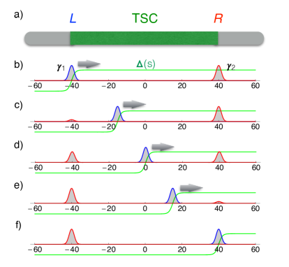
Figure 1: Majorana exchange in a 1D wire. a) Schematic depiction of the system with the central green region representing a TSC and outer regions an ordinary superconductor. Panels b-f) show the Majorana wavefunctions as the kink in $\Delta(s)$ (rendered in green) sweeps the wire from left to right.

In this Letter we introduce a simple protocol that allows for an exchange of two Majoranas in a single wire. The basic idea is illustrated in Fig. 1 and relies on the known fact that in the presence of an additional symmetry, such as time reversal, a kink in a TSC wire (defined as a $\pi$ domain wall in the phase of the superconducting order parameter) carries a protected pair of Majorana zero modes note2 ; fu79 ; tewari2 ; simon1 ; ojanen1 . As we show in detail below, under a wide range of conditions such a kink acts as a transport vehicle (“shuttle”) for the Majorana end modes. Specifically, as the kink traverses the wire from left to right it brings along with it the left end-mode (Fig. 1b,c). Meanwhile, the right end mode tunnels through the wire to its left end (Fig. 1d-e) so that the end result is an adiabatic exchange of two Majorana zero modes (Fig. 1f). We show that this exchange satisfies the usual rules of Ising braid group, namely

$$\gamma_{1}\mapsto\gamma_{2},\ \ \ \ \gamma_{2}\mapsto-\gamma_{1}.$$ (1)

We also discuss various limitations of our exchange protocol and its possible physical realizations.

Consider a process in which a $\pi$ domain wall is nucleated in the quantum wire Fig. 1a to the left of point $L$ and is then transported to the right along the wire. Initially, the domain wall is in the trivial superconductor and we do not expect it to bind any zero modes. We model this situation by the low-energy Hamiltonian

$$H_{0}=i\epsilon\Gamma_{1}\Gamma_{2},$$ (2)

where $\Gamma_{j}$ denote the Majorana operators that we anticipate to become zero modes once the kink reaches the TSC while $\epsilon$ is their energy splitting in the trivial phase. As the kink approaches the topological segment of the wire we expect two things to happen: (i) $\Gamma_{j}$ become zero modes, meaning we should set $\epsilon\to 0$ and (ii) since their wavefunctions begin to overlap with the wavefunction of $\gamma_{1}$, we expect terms $i\gamma_{1}\Gamma_{j}$ to enter (2) with non-zero coefficients.

Since the Hamiltonian (2) is invariant under a rotation in $(\Gamma_{1},\Gamma_{2})$ space, i.e. $\Gamma_{1}\to\Gamma_{1}\cos{\alpha}+\Gamma_{2}\sin{\alpha}$ and $\Gamma_{2}\to\Gamma_{2}\cos{\alpha}-\Gamma_{1}\sin{\alpha}$ we may, without loss of generality, select $\alpha$ such that the resulting Hamiltonian reads

$$H_{\rm I}=i\epsilon\Gamma_{1}\Gamma_{2}+it_{1}\gamma_{1}\Gamma_{2}.$$ (3)

This Hamiltonian reveals an important property of the system that will be key to the functioning of our device: as $\epsilon$ decays to zero and $t_{1}$ ramps up to a non-zero value, the zero mode denoted as $\gamma_{1}$ originally positioned at $L$ transforms into zero mode $\Gamma_{1}$ located at the kink. Physically, the kink subsumes the Majorana zero mode and transports it along the wire as illustrated in 1b,c. This is the key idea behind the Majorana shuttle.

As the kink approaches the center of TSC we can no longer ignore coupling $t_{2}$ to the other end mode denoted by $\gamma_{2}$. Indeed when the kink is exactly midway we expect $t_{1}=t_{2}$ on the basis of symmetry. The relevant Hamiltonian then becomes

$$H_{\rm II}=it_{1}\gamma_{1}\Gamma_{2}+it_{2}\gamma_{2}\Gamma_{2}.$$ (4)

As the kink advances along the wire and $t_{1}$ declines while $t_{2}$ grows the zero mode $\gamma_{2}$ transforms into $\gamma_{1}$. Physically, the zero mode initially located at $R$ tunnels across the length of the TSC and reappears on the other side at $L$.

Finally, as the kink traverses into the trivial phase to the right of the TSC the pair of ancillary Majoranas acquire a gap and $t_{2}$ reaches zero. We describe this by

$$H_{\rm III}=i\epsilon\Gamma_{1}\Gamma_{2}+it_{2}\gamma_{2}\Gamma_{2}.$$ (5)

As before, this shows that $\Gamma_{1}$ transforms into $\gamma_{2}$, completing the exchange.

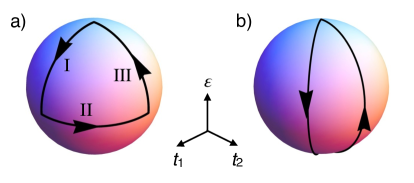
Figure 2: Parameter path ${\bf h}(s)$ on the unit sphere. a) The path representing Majorana shuttle exchange Eq. (Majorana fermion exchange in strictly one dimensional structures). b) An alternate exchange protocol discussed in Supplementary Material.

The entire sequence of events can be described economically by a single Hamiltonian note1

$$H(s)=i[t_{1}(s)\gamma_{1}+t_{2}(s)\gamma_{2}+\epsilon(s)\Gamma_{1}]\Gamma_{2}.$$ (6)

where $s$ represents the kink position along the wire, increasing from left to right. The spectrum of $H(s)$ consists of two exact zero modes and two non-zero energy levels $\pm E(s)=\pm\sqrt{t_{1}^{2}+t_{2}^{2}+\epsilon^{2}}$. Since we expect Majorana wavefunctions to decay exponentially at long distances a reasonable assumption inside TSC is $\epsilon(s)=0$ and $t_{1,2}(s)\approx t_{0}e^{(\pm s-l/2)/\xi}$ where $l$ is the TSC length, $\xi$ represents the decay length of the Majorana wavefunctions and $s$ is referenced to the TSC midpoint. This gives

$$E(s)\approx 2t_{0}e^{-l/2\xi}\sqrt{\cosh{(2s/\xi)}}.$$ (7)

It is useful to write the three couplings as a vector ${\bf h}(s)=(t_{1}(s),t_{2}(s),\epsilon(s))$, in spherical coordinates

$${\bf h}(s)=E(s)(\sin{\theta}\cos{\varphi},\sin{\theta}\sin{\varphi},\cos{\theta})$$ (8)

with angles $\theta$ and $\varphi$ dependent on $s$. The exchange can thus be visualized as a path on the unit sphere Fig. 2a parametrized by $[\theta(s),\varphi(s)]$; the amplitude $E(s)$ is unimportant as long as it remains non-zero.

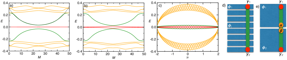
Figure 3: Lowest lying energy levels of the lattice Hamiltonian (12) with $\Delta=0.1t$ and $N=50$. a) Shown as a function of the kink position $M$ for $\mu=0.185t$ and b) for $\mu=0.140t$. The dashed line in panel a) represents the best fit of the second energy level to Eq. (7) with $t_{0}=0.246t$ and $\xi=9.20$. Panel c) displays the same energy levels as a function of the chemical potential $\mu$ with the kink fixed at the TSC midpoint $M=25$. Panels d,e) illustrate possible physical realizations of our device. Blue areas indicate SC electrodes with controlled phases $\phi_{j}$, green is the quantum wire with Majorana endmodes indicated in red.

The zero mode operators $\gamma(s)$ of the Hamiltonian (6) satisfy $[H(s),\gamma(s)]=0$ and correspond to two vectors ${\bm{v}}_{1}(s)$ and ${\bm{v}}_{2}(s)$ orthogonal to ${\bf h}(s)$. They read

$$\gamma_{1}(s) = \gamma_{1}\cos{\theta}\cos{\varphi}+\gamma_{2}\cos{\theta}\sin{\varphi}-\Gamma_{1}\sin{\theta}$$

$$\gamma_{2}(s) = -\gamma_{1}\sin{\varphi}+\gamma_{2}\cos{\varphi}$$ (9)

Of course any linear combination of $\gamma_{1}(s)$ and $\gamma_{2}(s)$ is also a zero mode of $H(s)$. The zero modes that solve the appropriate time-dependent Schrödinger equation are those linear combinations which make the non-Abelian Berry matrix $A_{ab}={\bm{v}}_{a}\cdot\partial_{s}{\bm{v}}_{b}$ vanish zee1 . With this in mind we can track the evolution of the zero modes as the couplings change. We do this in three stages as described by Hamiltonians $H_{\rm I}$, $H_{\rm II}$ and $H_{\rm III}$ above. The spherical angles evolve as

$$\theta: \ \ 0\stackrel{{\scriptstyle\rm I}}{{\longrightarrow}}{\pi\over 2}\stackrel{{\scriptstyle\rm II}}{{\longrightarrow}}{\pi\over 2}\stackrel{{\scriptstyle\rm III}}{{\longrightarrow}}0,$$

$$\varphi: \ \ 0\stackrel{{\scriptstyle\rm I}}{{\longrightarrow}}0\stackrel{{\scriptstyle\rm II}}{{\longrightarrow}}{\pi\over 2}\stackrel{{\scriptstyle\rm III}}{{\longrightarrow}}{\pi\over 2},$$ (10)

which implies, according to Eq. (Majorana fermion exchange in strictly one dimensional structures), the following evolution of the Majorana zero modes

$$\gamma_{1}(s): \ \ \gamma_{1}\stackrel{{\scriptstyle\rm I}}{{\longrightarrow}}-\Gamma_{1}\stackrel{{\scriptstyle\rm II}}{{\longrightarrow}}-\Gamma_{1}\stackrel{{\scriptstyle\rm III}}{{\longrightarrow}}\gamma_{2},$$

$$\gamma_{2}(s): \ \ \gamma_{2}\stackrel{{\scriptstyle\rm I}}{{\longrightarrow}}\ \ \gamma_{2}\stackrel{{\scriptstyle\rm II}}{{\longrightarrow}}-\gamma_{1}\stackrel{{\scriptstyle\rm III}}{{\longrightarrow}}-\gamma_{1}.$$ (11)

We observe that the exchange protocol indeed implements the Ising braid group Eq. (1).

The result shown in Eq. (Majorana fermion exchange in strictly one dimensional structures) is a direct consequence of the structure of the Hamiltonian (6) and is in that sense exact. However, in the derivation leading to our main result (Majorana fermion exchange in strictly one dimensional structures) we made an important assumption that in Hamiltonian (6) $\gamma_{2}$ only couples to $\Gamma_{2}$. This is non-generic because a term $it_{2}^{\prime}\gamma_{2}\Gamma_{1}$ is also allowed and cannot be removed by a rotation in $(\Gamma_{1},\Gamma_{2})$ space without generating additional undesirable terms. Such a coupling, when significant, spoils the exact braiding property Eq. (Majorana fermion exchange in strictly one dimensional structures) because it shifts the Majorana zero modes to non-zero energies $\pm t_{2}^{\prime}$ during step II. Parameter $t_{2}^{\prime}$ (like the remaining parameters in $H(s$)) depends on Majorana wavefunction overlaps and is therefore non-universal. In the following we study a simple lattice model for a TSC and show that the situation with $|t_{2}^{\prime}|$ much smaller than all the other relevant parameters can be achieved by tuning a single system parameter such as the chemical potential $\mu$ or the length $l$ of the topological segment of the wire. The necessity to tune $t_{2}^{\prime}$ to zero is the price one must pay in order to exchange Majoranas reliably in a 1D wire.

To put our ideas to the test we now study the $\pi$ kink in the prototype lattice model of TSC due to Kitaev kitaev1 . It describes spinless fermions hopping between the sites of a 1D lattice defined by the Hamiltonian

$${\cal H_{\rm latt}}=\sum_{j}\left[(-tc^{\dagger}_{j}c_{j+1}+\Delta_{j,j+1}c^{\dagger}_{j}c^{\dagger}_{j+1}+{\rm h.c.})-\mu c^{\dagger}_{j}c_{j}\right]$$ (12)

where $\Delta_{j,j+1}$ is the superconducting order parameter on the bond connecting sites $j$ and $j+1$. For non-zero uniform $\Delta_{j,j+1}$ the chain is known to be in a TSC phase when $|\mu|<|2t|$. Here we study an open ended chain with $N$ sites and a kink described as

$$\Delta_{j,j+1}=\biggl{\{}\begin{matrix}-\Delta,\ \ j\leq M\\ +\Delta,\ \ j>M\end{matrix}$$ (13)

In the limit of a long wire it is possible to find various zero mode wavefunctions analytically and from their matrix elements derive the effective Hamiltonian Eq. (6). Since the details of such calculations are tedious and not particularly illuminating we focus here on exact numerical diagonalizations which convey the key information with greater clarity. Figure 3a,b shows the energy eigenvalues of ${\cal H_{\rm latt}}$ as a function of the kink position $M$ for two typical and physically distinct situations. The four eigenvalues closest to zero (rendered in green and red) are associated with the Majorana modes $\gamma_{1},\gamma_{2},\Gamma_{1}$ and $\Gamma_{2}$ discussed above. In Fig. 3a we observe two near-zero modes (red) and two modes at finite energy behaving as expected from Eq. (7). For these chosen parameters the system behaves in accordance with our effective low-energy theory defined by the Hamiltonian $H(s)$ in Eq. (6). The inspection of the associated wavefunctions indeed confirms behavior indicated in Fig. 1b-f, fully consistent with the Majorana shuttle concept. For a slightly shifted chemical potential $\mu$ Fig. 3b shows that the zero modes are lifted, indicating that coupling $t_{2}^{\prime}$ has become significant. In this case the low-energy theory (6) does not apply and the adiabatic exchange is compromised.

To better understand the interplay between the two types of behavior contrasted in Fig. 3a,b we plot in panel c the energy spectrum of ${\cal H_{\rm latt}}$ as a function of the chemical potential for the kink fixed at the TSC midpoint $(M=N/2)$ where the difference is most pronounced. The oscillatory behavior of the energy levels here reflects the fact that in addition to the simple exponential decay Majorana wavefunctions also exhibit oscillations at the Fermi momentum $k_{F}$ of the underlying normal metal. These oscillations affect the wavefunction overlaps and thus influence the coupling constants in the effective Hamiltonian. If we denote the two lowest non-negative eigenvalues of ${\cal H_{\rm latt}}$ by $E_{0}(\mu)$ and $E_{1}(\mu)$ then, for the Majorana shuttle to function, we require that

$$E_{0}(\mu)\ll E_{1}(\mu).$$ (14)

When (14) is satisfied then one can perform the exchange operation sufficiently fast compared to $\hbar/E_{0}(\mu)$ so that the small energy splitting between the zero modes does not appreciably affect the result and at the same sufficiently slow compared to $\hbar/E_{1}(\mu)$ so that the condition of adiabaticity is satisfied and the system remains in the ground state. If on the other hand $E_{0}(\mu)$ and $E_{1}(\mu)$ are comparable then such an operation becomes impossible. In the wires used in the Delft experiment mourik1 the size of the Majorana wavefunction $\xi$ was estimated to be about $1/10$ of the wire length $l$. When the kink is near the wire midpoint one may thus crudely estimate $E_{1}(\mu)\simeq\ t(l/2\xi)e^{-l/2\xi}\simeq 0.3\Delta$. Parameters in our numerical simulations were chosen to yield comparable values. One may similarly estimate the typical maximum value of $E_{0}(\mu)$ for the situation when $\mu$ is appropriately tuned. This value would be zero in the ideal clean case and if we ignore the mutual overlap of the end-mode Majorana wavefunctions. Considering the latter to be non-zero we obtain $E_{0}(\mu)\simeq\ t(l/\xi)e^{-l/\xi}\simeq 0.0045\Delta$. We may thus conclude that with the existing wires and under favorable conditions the adiabaticity requirement $E_{0}(\mu)\ll E_{1}(\mu)$ can be satisfied with at least an order of magnitude to spare.

Inspection of Fig. 3c further reveals that a small adjustment of the average chemical potential $\mu$ should be sufficient in most cases to tune the system to satisfy Eq. (14). In essence, we require $\mu$ to be tuned close to one of the zeroes $\mu_{n}$ of $E_{0}(\mu)$. From Fig. 3c one can deduce a simple heuristic formula

$$E_{0}(\mu)\simeq f(\mu)\min(|\sin{k_{F}l}|,|\cos{k_{F}l}|)$$ (15)

with $f(\mu)$ a slowly varying envelope function. The zeroes occur at $k_{F}l={\pi\over 2}n$ with $n$ integer from which one can infer the spacing between the successive values of $\mu_{n}$ as $\delta\mu\approx\pi\mu/2N$. We see that if $\mu$ is initially set at random, for a long wire only a minute adjustment (achieved e.g. by gating) is required to bring it to the regime where adiabatic exchange using the Majorana shuttle protocol becomes feasible. In the Supplementary Material we furthermore show that the exchange protocol is robust with respect to moderate amounts of disorder in the chemical potential $\mu$, hopping $t$ and pairing amplitude $\Delta$. Specifically, the exchange occurs as long as the fluctuations in the above parameters do not significanly exceed the average pairing amplitude $\Delta_{0}$.

The Majorana shuttle can be physically realized by coupling a single semiconductor wire sau2 ; oreg1 ; mourik1 ; das1 ; deng1 ; finck1 ; churchill1 to a “keyboard” of superconducting electrodes as illustrated in Fig. 3d. If one can control the phases $\phi_{j}$ of the individual electrodes (e.g. by coupling them to flux loops) then a phase kink can be propagated along the wire in steps, implementing the proposed exchange protocol. It might be also possible to generate the kink by running a current between the adjacent electrodes in a variant of the setup discussed in romito1 ; large enough supercurrent should produce a phase difference close to $\pi$ owning to the fundamental Josephson relation $I(\Delta\phi)=I_{0}\sin{\Delta\phi}$.

An even simpler physical realization follows from the generalized exchange protocol discussed in the Supplementary Material. There we demonstrate that, as a matter of fact, an exchange of $\gamma_{1}$ and $\gamma_{2}$ is effected by any closed parameter path ${\bf h}(s)$ in the Hamiltonian (6) provided that (i) it starts at the pole of the unit sphere Fig. 2 and (ii) it sweeps a solid angle ${\pi\over 2}$. One such path, shown in Fig. 2b, can be physically realized in a setup with only two SC electrodes (San-Jose, ) indicated in Fig. 3e by simply twisting the phase of one of the electrodes by $2\pi$ (see Supplementary Material for details). As before, we require that endmodes $\gamma_{1}$ and $\gamma_{2}$ couple to the same ancillary Majorana, say $\Gamma_{2}$, localized in the juction. In addition, for the exchange to obey Eq. (1), it is necessary that $t_{1}=t_{2}$ to a good approximation, which can be implemented by positioning the junction midway along the wire.

Finally, we note that a pair of ancillary Majoranas is also realized at a magnetic domain wall in the chain of magnetic atoms deposited on the surface of a superconductor nadj-perge2 ; ojanen1 . Our exchange protocol works equally well in this situation, if a way can be found to manipulate the domain wall.

Our considerations demonstrate that it is in principle possible to exchange two Majorana fermions in a strictly one-dimensional system. The price one pays for this is the necessity to tune a single parameter (e.g. the global chemical potential) in the device. In the Majorana shuttle protocol one must in addition impose a symmetry constrain (such as the time reversal) to protect the Majorana doublet at the domain wall but this condition is relaxed in the Josephson junction implementation. Our proposed protocol involves four Majoranas, two of them ancillary, and relies on the fact that a pair of exact zero modes is preserved when only three of the four are mutually coupled. In steps I and III of the exchange this is guaranteed by virtue of the fourth Majorana being spatially separated from the remaining three. In step II one must tune a parameter to achieve the decoupling of the fourth Majorana. In this respect our protocol is similar to Coulomb assisted braiding heck1 but is potentially simpler to implement because it involves only a single quantum wire.

The authors are indebted to NSERC, CIfAR and Max Planck - UBC Centre for Quantum Materials for support.

References

- (1) J. Leinaas and J. Myrrheim, Nuovo Cimento B37, 1 (1977).
- (2) F. Wilczek, Phys. Rev. Lett. 48, 1144 (1982); ibid. 49, 957 (1982).
- (3) G. Moore and N. Read, Nucl. Phys. B 360, 362, (1991).
- (4) C. Nayak, S. H. Simon, A. Stern, M. Freedman, and S. Das Sarma, Rev. Mod. Phys. 80, 1083 (2008).
- (5) N. Read and D. Green, Phys. Rev. B61, 10267 (2000).
- (6) D.A. Ivanov, Phys. Rev. Lett. 86, 268 (2001).
- (7) A.Y. Kitaev, Phys. Usp. 44, 131 (2001).
- (8) J. Alicea, Rep. Prog. Phys. 75, 076501 (2012).
- (9) C.W.J. Beenakker, Annu. Rev. Con. Mat. Phys. 4, 113 (2013).
- (10) T. D. Stanescu and S. Tewari, J. Phys.: Condens. Matter 25, 233201 (2013).
- (11) L. Fu and C. L. Kane, Phys. Rev. Lett. 100, 096407 (2008).
- (12) J.D. Sau, R. M. Lutchyn, S. Tewari, and S. Das Sarma, Phys. Rev. Lett. 104, 040502 (2010).
- (13) J. Alicea, Phys. Rev. B81, 125318 (2010).
- (14) C. Kallin, Rep. Prog. Phys. 75, 042501 (2012).
- (15) R.M. Lutchyn, J.D. Sau and S. Das Sarma, Phys. Rev. Lett. 105, 077001 (2010).
- (16) Y. Oreg, G. Refael and F. von Oppen, Phys. Rev. Lett. 105, 177002 (2010).
- (17) V. Mourik, K. Zuo, S. M. Frolov, S. R. Plissard, E. P. A. M. Bakkers, and L. P. Kouwenhoven, Science 336, 1003 (2012).
- (18) A. Das, Y. Ronen, Y. Most, Y. Oreg, M. Heiblum, and H. Shtrikman, Nature Physics 8, 887 (2012).
- (19) M. T. Deng, C. L. Yu, G. Y. Huang, M. Larsson, P. Caroff, and H. Q. Xu, Nano Letters 12, 6414 (2012).
- (20) A. D. K. Finck, D. J. Van Harlingen, P. K. Mohseni, K. Jung, and X. Li, Phys. Rev. Lett. 110, 126406 (2013).
- (21) H. O. H. Churchill, et al., Phys. Rev. B87, 241401 (2013).
- (22) E. J. H. Lee, X. Jiang, M. Houzet, R. Aguado, C. M. Lieber, and S. D. Franceschi, Nature Nanotechnology, 9, 79, (2014).
- (23) J. Alicea, Y. Oreg, G. Refael, F. von Oppen, M.P.A. Fisher, Nature Phys. 7, 412 (2011).
- (24) B. van Heck, A.R. Akhmerov, F. Hassler, M. Burrello, and C.W. J. Beenakker, New J. Phys. 14, 035019 (2012).
- (25) K. Flensberg, Phys. Rev. Lett. 106, 090503 (2011)
- (26) J.D. Sau, D.J. Clarke, and S. Tewari, Phys. Rev. B84, 094505 (2011)
- (27) A 1D system obeying both the particle-hole and time-reversal symmetry is in BDI topological class characterized by an integer-valued invariant . Segments with the opposite sign of the SC order parameter have and a domain wall thus binds two Majorana fermions.
- (28) L. Fu and C.L. Kane, Phys. Rev. B79, R161408 (2009).
- (29) S. Tewari and J.D. Sau, Phys. Rev. Lett. 109, 150408 (2012).
- (30) D. Sticlet, C. Bena, and P. Simon, Phys. Rev. B87, 104509 (2013)
- (31) K. Pöyhönen, A. Westström, J. Röntynen, and T. Ojanen, arXiv:1308.6108
- (32) We note that this Hamiltonian has been studied previously in the context of Coulomb assisted braiding in Ref. heck1 .
- (33) F. Wilczek and A. Zee, Phys. Rev. Lett. 52, 24 (1984).
- (34) A. Romito, J. Alicea, G. Refael, and F. von Oppen, Phys. Rev. B85, 020502(R) (2012).
- (35) S. Nadj-Perge, I.K. Drozdov, B.A. Bernevig, A. Yazdani, Phys. Rev. B88, 020407 (2013).
- (36) P. San-Jose, E. Prada, and R. Aguado, Phys. Rev. Lett. 108, 257001 (2012)