The Density and Mass of Unshocked Ejecta in Cassiopeia A through Low Frequency Radio Absorption

Abstract

Characterizing the ejecta in young supernova remnants is a requisite step towards a better understanding of stellar evolution. In Cassiopeia A the density and total mass remaining in the unshocked ejecta are important parameters for modeling its explosion and subsequent evolution. Low frequency ($<$100 MHz) radio observations of sufficient angular resolution offer a unique probe of unshocked ejecta revealed via free-free absorption against the synchrotron emitting shell. We have used the Very Large Array plus Pie Town Link extension to probe this cool, ionized absorber at 9$\arcsec$ and 18$\farcs$5 resolution at 74 MHz. Together with higher frequency data we estimate an electron density of 4.2 cm^-3 and a total mass of 0.39 M_☉ with uncertainties of a factor of $\sim$2. This is a significant improvement over the 100 cm^-3 upper limit offered by infrared [S III] line ratios from the Spitzer Space Telescope. Our estimates are sensitive to a number of factors including temperature and geometry. However using reasonable values for each, our unshocked mass estimate agrees with predictions from dynamical models. We also consider the presence, or absence, of cold iron- and carbon-rich ejecta and how these affect our calculations. Finally we reconcile the intrinsic absorption from unshocked ejecta with the turnover in Cas A’s integrated spectrum documented decades ago at much lower frequencies. These and other recent observations below 100 MHz confirm that spatially resolved thermal absorption, when extended to lower frequencies and higher resolution, will offer a powerful new tool for low frequency astrophysics.

1. Introduction

1.1. General Background on Cas A

Cassiopeia A (Cas A; 3C 461, G111.7-2.1) is the 2nd-youngest-known supernova remnant (SNR) and, at a distance of 3.4 kpc (Reed et al., 1995), it lies just beyond the Perseus Arm of the Galaxy. With the discovery of light echoes from the explosion, we now know that Cas A resulted from a type IIb explosion (Krause et al., 2008). Cas A is one of the strongest synchrotron radio-emitting objects in the sky and has been observed extensively with the Very Large Array (VLA) since its commissioning in 1980.

The morphology of Cas A is quite complex with structure distributed over a variety of spatial scales. The terminology used to describe some of these structures was coined in some of the earliest papers describing the optical and resolved radio images (van den Bergh & Dodd, 1970; Ryle, Elsmore, & Neville, 1965). The most prominent feature is the almost circular “Bright Ring” at a radius of $\approx 100\arcsec$ which is generally regarded as marking the location of ejecta that have interacted with the reverse shock (see e.g. Morse et al., 2004). A fainter “plateau” of radio emission is seen out to a radius of $\approx 150\arcsec$. To the northeast, where the shell becomes broken, is the “jet” and extending in the opposite direction to the southwest is the counter-jet. The jet and counter-jet do not represent outflow in the classical sense. Instead they describe locations where the fastest-moving ejecta are observed well beyond the plateau and farthest from the explosion center (see e.g. Hammell & Fesen, 2008). To the southeast, iron-rich ejecta extend beyond the Bright Ring and into the plateau. The jets and extended iron-rich structure are likely the result of an asymmetric explosion of the progenitor (see e.g. Hughes et al., 2000; Hwang & Laming, 2012). The light echo data also indicate an asymmetric explosion (Rest et al., 2011).

1.2. Unshocked Ejecta

In addition to the shocked ejecta described above, there is a class of ejecta still interior to the reverse shock in Cas A. These “unshocked ejecta” were discovered via absorption of low frequency ($<$100 MHz) radio emission (Kassim et al., 1995) and are also seen to radiate in the infrared in the emission lines of [O IV], [S III], [S IV], and [Si II] (Ennis et al., 2006). The term “unshocked” is somewhat of a misnomer because all of the ejecta were originally shocked by the passage of the blast wave through the star. However, the ejecta cooled during the subsequent expansion of the SNR. What we consider to be shocked ejecta today are those ejecta that have crossed through the reverse shock with the term “unshocked ejecta” referring to those ejecta that are still interior to the reverse shock. Thus the simple cartoon of Cas A’s structure is that of cold ejecta in the interior of a roughly spherical shell composed of shocked gas that radiates strongly in multiple bands. At low frequencies, the radio emission from the far side of the shocked shell is absorbed by the cold, unshocked ejecta in the interior. In §5.4 we provide a more thorough description of the geometry assumed for our analysis.

The infrared emission from the unshocked ejecta in Cas A occurs because they have been photoionized. An analysis of the unshocked ejecta observed in the supernova remnant SN1006, based on calculations of photoionization cross-sections and Bethe parameters, showed that the unshocked ejecta are photoionized by two primary sources (Hamilton & Fesen, 1988). Ambient ultraviolet starlight is all that is necessary to photoionize Si I and Fe I since their ionization potentials are below the Lyman limit. For ions with ionization potentials above the Lyman limit, the ultraviolet and soft X-ray radiation field of the shocked ejecta in SN1006 is such that species up to O III (54.9 eV), Si IV (45.1 eV), and Fe IV (54.8 eV) can be photoionized. A similar analysis was performed for Cas A assuming photoionization equilibrium, abundances appropriate for a core-collapse SNR, a thermal bremsstrahlung spectrum for the shocked ejecta, and utilizing a simple one-dimensional hydrodynamic model to follow Cas A’s evolution (Eriksen, 2009). This simplified model predicts that [Si II] (34.8µm) and [O IV] (25.9µm) should be the dominant infrared lines in the unshocked ejecta, directly in line with observations (Ennis et al., 2006). In addition, Eriksen (2009) predicts strong [O III] (88.4µm), which we will show in §5.3 is present in spectra from the Infrared Space Observatory (ISO, Unger et al., 1997; Docenko & Sunyaev, 2010).

Cas A was spectrally mapped with the Spitzer Space Telescope and Doppler shifts were measured which allowed a 3D mapping of the ejecta distribution, including the unshocked component (DeLaney et al., 2010; Isensee et al., 2010). We now know based on the Spitzer data that the ejecta are organized into a “thick disk” structure, tilted at $\sim 70\arcdeg$ from the line-of-sight, providing further evidence that the explosion, or subsequent evolution of the SNR prior to the reverse shock encounter, must have been asymmetric. An upper limit of 100 cm^-1 was determined for the electron density of the unshocked ejecta based on infrared [S III] line ratios, but the actual density is likely much lower (Eriksen, 2009; Smith et al., 2009).

The absorption seen in the low frequency radio observations provides a means to probe the density and mass of the unshocked ejecta because the free-free optical depth ($\tau_{\nu}$) is related to emission measure and thus density. Kassim et al. (1995) attempted to determine the total mass of the unshocked ejecta, but due to using a $\tau_{\nu}$ appropriate for a hydrogenic gas and a temperature that was too high, arrived at 19M_☉, which is unreasonably large considering that the total ejecta mass is likely only 2-4 M_☉ (Hwang & Laming, 2012). Given the role that the ejecta play in the evolution of SNRs, it is important to provide an accurate census of the total mass present, thus prompting a new look at the low frequency absorption analysis of Kassim et al. (1995).

1.3. Low Frequencies on the VLA

1.3.1 Low Frequencies on the Legacy VLA

The upgraded Karl G. Jansky Very Large Array (VLA) primarily accesses frequencies above 1 GHz through its broadband Cassegrain focus systems. Its predecessor, hereafter the “legacy” VLA, also accessed two relatively narrow bands below 1 GHz through its primary focus systems (Kassim et al., 1993, 2007). These included the “P band” and “4 band” systems operating at 330 MHz (1990-2009) and 74 MHz (1998-2009), respectively. Both systems provided sub-arcminute resolution imaging and were widely used over their lifetimes. These systems were removed during the VLA upgrade and have been only recently replaced with a new “Low Band” receiving system (Clarke et al., 2011). The first call for proposals using the 330 MHz band of this new system was issued by NRAO in February, 2013.

1.3.2 Pie Town Link

The legacy 74 MHz and 330 MHz VLA systems achieved their maximum angular resolution of $\sim 20\arcsec$ and $\sim 6\arcsec$ in the A configuration (maximum baseline $\sim$36 km), respectively. An 8-antenna prototype of the 74 MHz system was used to observe Cas A (Kassim et al., 1995) early on, adding to the body of VLA work extending from 330 MHz to higher frequencies. As the resolution was still relatively poor compared to shorter wavelengths, NRL and NRAO added a 74 MHz feed system to the Pie Town antenna, utilizing an optical fiber link connecting the innermost Very Large Baseline Array (VLBA) antenna to the legacy VLA. With a maximum baseline of 73 km, this improved the angular resolution at 74 MHz and 330 MHz by a factor of two to approximately 9$\arcsec$ and 3$\arcsec$ respectively. Cas A was thereafter reobserved with the full (27-antenna) 74 MHz and the 330 MHz legacy systems using the Pie Town link capability in August 2003.

1.4. This Paper

In this paper, we report on legacy VLA observations in 1997-1998 at frequencies of 5 GHz, 1.4 GHz, 330 MHz, and 74 MHz, and on the Pie Town link, observations at frequencies of 330 MHz and 74 MHz in 2003. We use our derived images to determine the degree of free-free absorption present, applying the appropriate formula for when the composition of the gas is not dominated by hydrogen. Finally, we calculate the density and mass of the unshocked ejecta and discuss the implications of our results.

2. Observations and Imaging

2.1. 1997-1998 and 2003 Legacy VLA Observations and Calibration

Observations were made with the legacy VLA in 1997 and 1998 using all four configurations from the most extended A-configuration with a maximum antenna separation of 36.4 km to the most compact D-configuration with a shortest separation of 35 m. These are summarized in Table 1. Data were taken at 4410.0, 4640.0, 4985.0, and 5085.0 MHz (hereafter called 5 GHz or C band), at 1285.0, 1365.1, 1464.9, and 1665.0 MHz (hereafter called 1.4 GHz or L band), at 327.5 and 333.0 MHz (hereafter called 330 MHz or P band), and at 73.8 MHz (hereafter called 74 MHz or 4 band). The 5 GHz and 1.4 GHz data were taken in continuum mode with pairs of frequencies observed simultaneously. The purpose of observing at multiple 5 GHz and 1.4 GHz bands is to improve sensitivity while avoiding bandwidth smearing. The 330 MHz and 74 MHz data were taken in spectral line mode. Note that the D-configuration data taken at 330 MHz and 74 MHz had insufficient resolution to be useful for this paper and were not utilized.

In order to increase the spatial resolution of the lowest frequency images, further observations at 74 MHz and 330 MHz were taken with the legacy VLA in A-configuration and utilizing the Pie Town (PT) link (hereafter called A+PT). We were allocated an 18-hour observing block in Aug 2003 with 12.2 hours on Cas A and the remainder of the time on calibrators and other sources of interest at low frequencies. The 2003 observations are also summarized in Table 1.

Table 1 Cas A 1997-1998 and 2003 Legacy VLA Observations

				On-Source Time
			Bandwidth	per Band
Date	Configuration	Band	(MHz)	(minutes)
1997 May	B	4	1.5625	33
		P	3.125	67
		L	12.5	241
		C	12.5	293
1997 Sep	C	4	1.5625	24
		P	3.125	24
		L	12.5	144
		C	12.5	142
1997 Nov, Dec	D	4	1.5625	14
		P	3.125	14
		L	12.5	84
		C	12.5	123
1998 Mar	A	4	1.5625	61
		P	3.125	61
		L	6.25	464
		C	6.25	467
2003 Aug	A+PT	4	1.5625	732
		P	3.125	732

Standard calibration procedures at 1.4 and 5 GHz were used for the data as described in the AIPS Cookbook. Primary flux calibration was based on the source 3C 48, the polarization calibrator was 3C 138, and the phase calibrator was J2355+4950. After initial calibration, multiple passes of self-calibration and imaging were performed on the Cas A data to improve the antenna phase and gain solutions.

The observations at 330 MHz and 74 MHz were performed in spectral line mode due to the presence of narrow-band radio frequency interference (RFI). Images of Cygnus A at 330 MHz and 74 MHz, after normalization to the Baars et al. (1977) absolute flux density scale, were used for both flux and bandpass calibration. RFI was flagged out and the data were combined into a single channel at each band. Iterative cycling between self calibration and imaging was then used to improve the phase and gain solutions for Cas A and to derive the final images.

74 MHz legacy VLA data, especially for the B, A, and A+PT link configurations, require corrections for ionospheric phase variations that can be rapid and severe over baselines longer than several kilometers (Kassim et al., 2007). Fortunately, Cas A so completely dominates the visibility phase measurements that straightforward self-calibration, yielding one phase correction per antenna, is perfectly capable of measuring the ionospheric effects. Moreover, the signal-to-noise is sufficiently high that the fluctuations can be tracked and corrected at the native sampling rate of 6.7 seconds.

Standard 74 MHz and 330 MHz data reduction also typically requires wide-field, multi-faceted imaging of spectral line data, to address non-coplanar baseline imaging and bandwidth smearing, respectively (Kassim et al., 2007). Fortunately, Cas A is of small angular size (only $\sim 300\arcsec$ across) such that there is no need for implementing angular-dependent gain solutions nor dealing with the non-coplanar array. Furthermore, Cas A is so strong that the contribution of other sources in the primary beams at both frequencies is negligible, and hence neither technique was required, greatly simplifying the data reduction.

2.2. Total Intensity Images

Table 2 Final Image Statistics

		$u$-$v$ range	$\theta_{LAS}$	FOV	Noise	Dynamic	$S_{\nu}$	$\delta S_{\nu}$
Band	Epoch	(k$\lambda$)	(arcsec)	(arcmin)	(mJy bm-1)	Range	(Jy)	(Jy)
2$\farcs$5 Resolution
P	2003	0.7-81	170	150	5.5	40	6217	124
L	1997/8	0.5-81	300	30	1.8	193	2204	44
C	1997/8	0.5-81	300	7.5	3.2	194	809	16
9″ Resolution
4	2003	0.7-18	170	600	190	368	18951	379
P	2003	0.7-18	170	150	26	135	6217	124
18$\farcs$5 Resolution
4	1997/8	0.12-9	800	600	387	513	18555	371
P	1997/8	0.5-9	300	150	94	267	6185	124
		(0.12-9)					(5859)
L	1997/8	0.12-9	800	30	21	249	2179	44

We present in this section sets of “matched” images at 2$\farcs$5, 9″, and 18$\farcs$5 resolution. The individual configuration data at each band were concatenated and images made with matched beam sizes. Minimum and maximum spatial frequency ($u$-$v$) ranges were used to match spatial sampling with the exception of the 2$\farcs$5 and 18$\farcs$5 330-MHz images which have a different minimum $u$-$v$ cutoff than the other images due to the native minimum $u$-$v$ distance for the 2003 A+PT data and to avoid the Van Vleck bias for the 1997-1998 data, as discussed below. The AIPS maximum-entropy deconvolution routine VTESS was used to restore the total intensity images. The default image for VTESS was a 5 GHz image of appropriate spatial resolution. Using the same default image in VTESS for all of the bands essentially forces the images to look as much alike as possible, with any resulting differences being due to the requirements of the data. Initial zero-spacing flux guesses were supplied to VTESS based on the 5 GHz integrated flux density and Cas A’s average spectral index of -0.77. The “negative flux” option was used so that VTESS was not required to get within 5% of the flux estimate. The standard correction for primary beam attenuation was applied to all of the final images. Since there were four images at 1.4 GHz and four images at 5 GHz, the images for each band needed to be normalized in flux density and averaged together. While we could have concatenated the final calibrated $u$-$v$ datasets and then performed the imaging, we chose to normalize the images directly. There are two primary reasons for this choice. First, the slightly different primary beam correction at each band introduces a small, but not insignificant error. Second, it is generally not a good idea to force the $u$-$v$ data to the same flux density, and grid on one plane for objects, such as Cas A, that have significant spectral gradients because each $u$-$v$ cell has a slightly different visibility amplitude at each band. Furthermore, since the individual 5 GHz and 1.4 GHz bands are close together, the relative calibration uncertainty is large enough that Cas A’s well-known average spectral index cannot be used to scale between them. This necessitates doing the concatenation and normalization in the imaging plane. We determined the average scaling factor between each set of 5 GHz and 1.4 GHz images using the radial surface brightness profiles extracted from a series of 20° wedges. The 1.4 GHz images were scaled to the 1.285 GHz image and the 5 GHz images were scaled to the 4.64 GHz image. In Table 2, we summarize the integrated flux densities, noise figures, and $u$-$v$ ranges for the final images and in Figure 1 we plot the integrated radio spectrum of Cas A. The uncertainty in the integrated flux density at each band is calculated based on a 2% uncertainty in the absolute flux scale of the VLA (Perley & Taylor, 1991).

Figure 1.— Integrated flux density measurements at each of the four observing bands and using the $u$-$v$ ranges indicated in Table 2. The error in flux density is 2%, which is much smaller than the plotting symbols. The filled triangles indicate the flux densities of the 1997-1998 1.4 GHz and 330 MHz images using their native minimum $u$-$v$ distances to demonstrate the magnitude of the Van Vleck bias in each. The dotted line represents a spectral index of -0.77.

At 330 MHz, legacy VLA observations of Cas A suffer from the Van Vleck bias (Van Vleck & Middleton, 1966) which depends very strongly and non-linearly on the correlated flux density and also affects phase since the degradation operates independently on the real and imaginary portions of the visibility separately. Thus, short antenna spacings report a reduced flux density which skews the final reconstructed flux density of the image by about 6% as shown in Table 2 and Figure 1. An effect this large would create a significant bias in spectral index and absorption measurements. For the A+PT 330 MHz data taken in 2003, the minimum $u$-$v$ distance is 0.7 k$\lambda$, which is long enough to avoid the Van Vleck bias. In order to avoid this bias for the 1997-1998 330 MHz image, which has data from shorter baselines, we impose a 0.5 k$\lambda$ minimum to the $u$-$v$ range. This limit happens to correspond to the minimum baseline for the 5 GHz data in D-configuration and results in a completely negligible Van Vleck bias (Thompson, Moran, & Swenson, 2007). Unfortunately, variations in spatial sampling between images can affect spectral index measurements. Different deconvolution methods provide different abilities to “fill in” the holes in the $u$-$v$ sampling. Strict overlap or matching of $u$-$v$ coverage is not required to get a good image, especially for an exceptionally bright source such as Cas A. Furthermore, good deconvolution algorithms are able to recover the short-spacing flux, especially when they permit a total flux estimate and allow a default image, as VTESS does.

The Van Vleck bias also should affect the 1.4 GHz images based on the correlation coefficient (Thompson, Moran, & Swenson, 2007), however we note only a 1% difference in the total flux density when using 0.5 k$\lambda$ vs. 0.12 k$\lambda$ as the minimum of the $u$-$v$ range (0.12 k$\lambda$ corresponds to the minimum baseline for the 1.4 GHz data in D-configuration.) The 1% flux density difference at 1.4 GHz is small enough that other factors besides the Van Vleck bias might be accountable.

The integrated spectrum of Cas A plotted in Figure 1 shows that the spectral index ($\alpha_{\nu_{1}}^{\nu_{2}}\equiv\log(S_{1}/S_{2})/\log(\nu_{1}/\nu_{2})$) is constant from 5 GHz up to 330 MHz ($\alpha_{330}^{1.4}=-0.76\pm 0.01$ and $\alpha_{1.4}^{5}=-0.77\pm 0.01$) when using a minimum $u$-$v$ cutoff for the 330 MHz image. From 330 MHz to 74 MHz, the integrated spectrum flattens slightly ($\alpha_{74}^{330}=-0.74\pm 0.01$). The uncertainties in spectral index are calculated based on a formal propagation of the uncertainty in integrated flux density, and thus the spectral flattening at 74 MHz is statistically significant. The spectral index between 5 GHz and 330 MHz is the same as that reported by Baars et al. (1977) for epoch 1980 but the spectral index between 330 MHz and 74 MHz is steeper than the 1980 result. Baars et al. (1977) derived a frequency-dependent secular decrease in flux density which would flatten the spectral index over time. Newer low frequency observations have shown that there is no frequency dependence to the secular decrease and the overall rate is about 8% yr^-1 (Rees, 1990; Helmboldt & Kassim, 2009). The integrated flux densities we report in Table 2 at 5 GHz, 1.4 GHz, and 330 MHz are only $\sim$3% less than the 1980 values from Baars et al. (1977) and the 74 MHz integrated flux densities are largely consistent with those reported by Helmboldt & Kassim (2009). There is no significant change in integrated flux density between 1997-1998 and 2003. Given the differences in aperture coverage, constraints imposed during image reconstruction, and flux standards applied for the different data sets, as well as the short-term variability observed in Cas A (Anderson & Rudnick, 1995; Helmboldt & Kassim, 2009), our flux densities are in line with expectations. Thus we argue that there is no significant curvature in Cas A’s integrated spectrum between 5 GHz and 330 MHz but there is a significant flattening of the integrated spectrum at lower frequencies.

We did not concatenate the 1997-1998 and 2003 data sets in order to make images containing data from both epochs because of two complicating factors. The first is the non-negligible proper-motion induced shift, due to expansion, across the epochs, and the second are the variations in the brightness of compact features over time. Anderson & Rudnick (1995), for example, found that two-thirds of the compact radio features in Cas A have brightness changes in the range of -2.2% yr^-1 to +5.2% yr^-1 and that the compact features were on average brightening at the rate of 1.6% yr^-1. At low spatial resolution, the proper motions and small-scale brightness changes are mitigated, but then there is no reason to combine the A+PT data with the lower resolution data except to improve signal-to-noise, which as we will demonstrate below, was not necessary for the analysis at 18$\farcs$5 resolution.

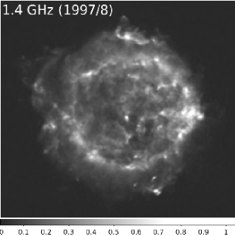
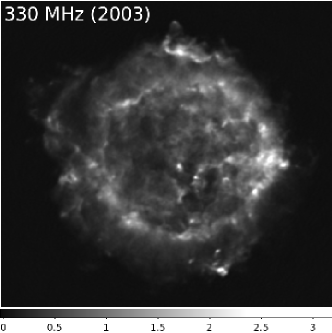
Figure 2.— 5 GHz (top) and 1.4 GHz (middle) images of Cas A from 1997-1998 and 330 MHz image (bottom) from 2003. The resolution is 2$\farcs$5 and the flux density scales are in Jy bm^-1. The $u$-$v$ ranges used to construct these images and the noise and integrated flux densities are reported in Table 2.

2.2.1 2$\farcs$5 Resolution Images

Figure 2 shows the final 1997-1998 5 GHz and 1.4 GHz images and the 2003 330 MHz image at 2$\farcs$5 resolution. With the improved resolution using the Pie Town link, we can see that the 330 MHz image captures the same large- and small-scale features as at higher frequencies, thus supporting the constant spectral index found from 5 GHz to 330 MHz. The dynamic range of the 330 MHz image is on par with the 1.4 GHz image and noticeably better than the 5 GHz image. The relatively poor dynamic range of the 5 GHz image is partly because the primary beam of the VLA at 5 GHz is only 1.5 times larger than Cas A, as indicated in Table 2. The high quality of the 330 MHz image demonstrates how well the AIPS task FLGIT excises RFI and the power of self-calibration for dealing with ionospheric effects.

2.2.2 9″ Resolution Images

Figure 3 shows the final 2003 330 MHz and 74 MHz images at 9″ resolution, which is the best resolution achieved with the A+PT link at 74 MHz. The dynamic range on the 330 MHz image is about 3 times better than for the 74 MHz image. Clumpy structure is observed on a variety of spatial scales down to the resolution limit. Comparing to the 2$\farcs$5 resolution images in Figure 2, it is clear that the same synchrotron features are responsible for the emission at 74 MHz. The bottom panel of Figure 3 is a plot of the angle-averaged radial surface brightness profiles of the 330 MHz and 74 MHz images. The profiles have been normalized to their peak values. The emission in the center of the 74 MHz image is noticeably fainter than expected based on the appearance of the 330 MHz image and therefore contributes to the flattening of the integrated spectrum from 330 MHz to 74 MHz observed in Figure 1.

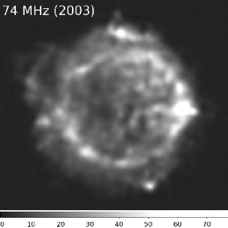
Figure 3.— Top and middle: 2003 A+PT configuration images of Cas A at 330 MHz and 74 MHz. The resolution is 9″. The flux density scales are in Jy bm^-1. The $u$-$v$ ranges used to construct these images and the noise and integrated flux densities are reported in Table 2. Bottom: Angle-averaged radial surface brightness profiles of the 330 MHz and 74 MHz images normalized to their peak values.

2.2.3 18$\farcs$5 Resolution Images

Figure 4 shows the final 1.4 GHz, 330 MHz and 74 MHz images at 18$\farcs$5 resolution from the 1997-1998 observations. This represents the best resolution attained with the legacy VLA in A-configuration at 74 MHz. The dynamic range on the 1.4 GHz image is about 2 times better than for the 330 MHz and 74 MHz images. The 74 MHz image at this lower resolution has a dynamic range about twice that at higher resolution using the A+PT link. The higher dynamic range allows us to better probe the large-scale diffuse emission from Cas A. The absorption of emission from the center of Cas A is, again, clearly observed.

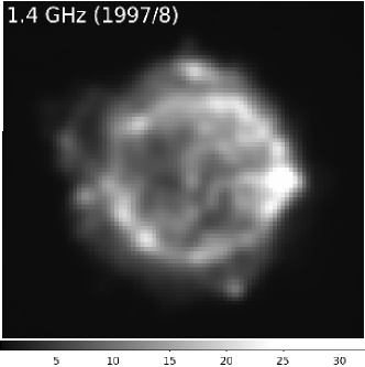
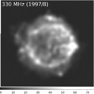
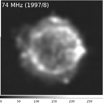
Figure 4.— 1.4 GHz (top left), 330 MHz (top right), and 74 MHz (bottom left) images of Cas A from 1997-1998. The resolution is 18$\farcs$5 and the flux density scales are in Jy bm^-1. The $u$-$v$ ranges used to construct these images and the noise and integrated flux densities are reported in Table 2. The angle-averaged radial surface brightness profiles of the 330 MHz and 74 MHz normalized to their peak values are shown at bottom right.

3. Spectral Index Imaging Analysis

3.1. Spectral Index at 9″ Resolution

The 2003 330 MHz and 74 MHz images at 9″ resolution were combined to form the spectral index image shown in Figure 5. Only spectral index data from regions greater than 10-$\sigma$ on the 330 MHz image were retained. The range of spectral indices at 9″ resolution is $\alpha_{74}^{330}\approx$-0.95 to -0.35, with the flattest spectrum corresponding to the bright clump in the center of Cas A. Anderson et al. (1991) report an average $\alpha_{1.4}^{5}\approx$-0.78 for the collection of clumps in that location, thus a significant spectral flattening has occurred.

The abundance of clumps with flat (blue) spectral indices in the center are not necessarily an indication of absorption. Many of the central clumps are known to have flat spectral indices based on images at higher frequencies (Anderson et al., 1991). In order to assess the degree of absorption in Cas A, we need to look at the difference in spectral index from high frequencies to low frequencies. Since we did not take higher frequency data with the 2003 observations, and the proper motion and small-scale brightness variations across epochs would be evident at 9″ resolution, we must work with our lower resolution images.

3.2. Spectral Index at 18$\farcs$5 Resolution

The 1997-1998 74 MHz, 330 MHz, and 1.4 GHz images at 18$\farcs$5 resolution were combined to form the spectral index images presented in Figure 6. Only spectral index data from regions greater than 10-$\sigma$ on the 330 MHz image were retained. These images show similar patterns in spectral index as those presented by Kassim et al. (1995) at 25″ resolution but at higher signal-to-noise for the images tied to 74 MHz because of the full complement of antennas available. As with the higher resolution spectral index image in Figure 5, the central features in the $\alpha_{74}^{330}$ image are notably flatter than the Bright Ring. One distinct advantage at lower spatial resolution is that the signal-to-noise is high enough to probe the spectral index of the diffuse emission as well as the clumped emission. The range of spectral indices between 330 MHz and 1.4 GHz (Figure 6 left) is $\alpha_{330}^{1.4}\approx$-0.85 to -0.65 and is typical of that observed at higher frequencies (Anderson et al., 1991). The range of spectral indices between 74 MHz and 330 MHz (Figure 6 right) is $\alpha_{74}^{330}\approx$-0.95 to -0.5, which is slightly larger than that between 330 MHz and 1.4 GHz. Both images in Figure 6 are plotted using the same spectral index scale in order to better demonstrate the spectral flattening effect in the central regions of the $\alpha_{74}^{330}$ image. At 18$\farcs$5 resolution, the central region is not as flat as at 9″ resolution. This could be because the lower resolution smooths out large variations and also because of the lower dynamic range of the 9″ resolution image.

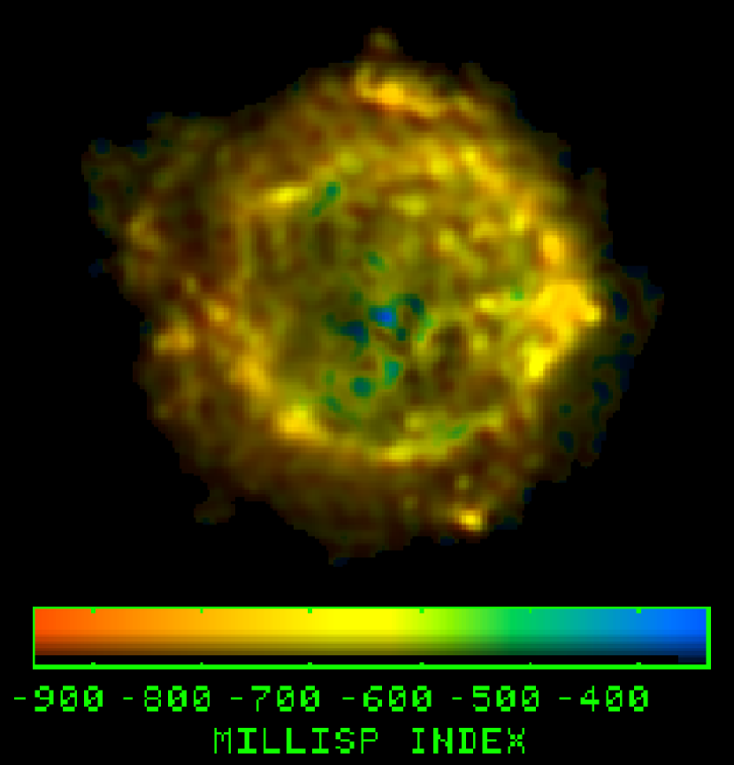
Figure 5.— Spectral index image between 74 MHz and 330 MHz made from the 2003 data set. Only spectral index data from regions greater than 10-$\sigma$ on the 330 MHz image are shown. The 330 MHz image is used as a brightness channel to illuminate the spectral index colors. The resolution is 9″.

As noted by Kassim et al. (1995), the spectral indices for features on the Bright Ring are about the same from high frequencies to low frequencies. At the center of Cas A, however, there is a significant flattening of the spectral index between 330 MHz and 74 MHz. Given that the spectral flattening is confined to the center of the 74 MHz image, there is likely an absorbing medium in or near Cas A that affects the observed low frequency emission but not the observed high frequency emission.

3.3. Spectral Index Difference ($\Delta\alpha$)

The spectral index variations observed at high frequencies reflect the different energy spectra of accelerated electron populations. These different energy spectra may be due to the acceleration at the forward and reverse shocks and to intrinsic breaks in the underlying electron energy spectrum (Anderson et al., 1991). The spectral index variations observed at low frequencies are due to both the accelerated electron populations and effects from free-free absorption.

In order to isolate spectral changes due only to free-free absorption, we assume that there is no curvature in the emitted synchrotron spectrum at low frequencies. Thus, when we subtract the two spectral index images, the resulting image, $\Delta\alpha=\alpha_{74}^{330}-\alpha_{330}^{1.4}$, shows only variations due to free-free absorption. Our $\Delta\alpha$ image is shown in Figure 7 with the same signal-to-noise cutoff as the spectral index images. The 330 MHz image was again used to illuminate the colors. Typical $\Delta\alpha$ values for regions with good S/N ratio vary from -0.1 to 0.25 where positive $\Delta\alpha$ indicates absorption and statistical variations due to noise are of order $\pm$0.01 to 0.02. Most of the free-free absorption is confined to the middle of Cas A with typical $\Delta\alpha$ values of 0.1-0.25. This is the same absorption morphology noted by Kassim et al. (1995) who found a peak $\Delta\alpha$=0.3 with their 25″ resolution images.

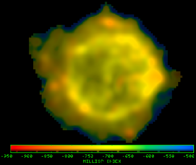
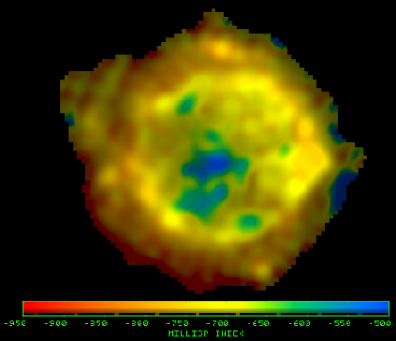
Figure 6.— Spectral index images between 330 MHz and 1.4 GHz (top) and between 74 MHz and 330 MHz (bottom) made from the 1997-1998 data set. Only spectral index data from regions greater than 10-$\sigma$ on the 330 MHz image are shown. The 330 MHz image is used as a brightness channel to illuminate the spectral index colors. The resolution is 18$\farcs$5.

4. Comparison with Infrared Emission from Unshocked Ejecta

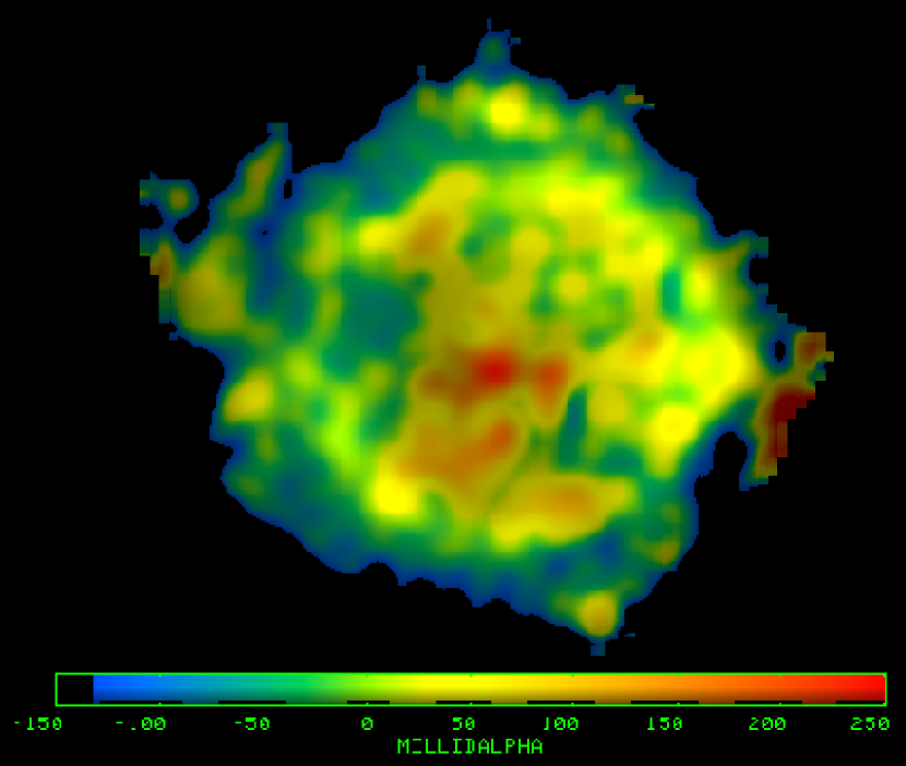
Figure 7.— Spectral index difference ($\Delta\alpha$ or dalpha) between $\alpha_{74}^{330}$ and $\alpha_{330}^{1.4}$. Only spectral index data from regions greater than 10-$\sigma$ on the 330 MHz image are shown. The 330 MHz image is used as a brightness channel to illuminate the $\Delta\alpha$ colors. The resolution is 18$\farcs$5. The orange and red colors indicate locations with free-free absorption.

One of the most exciting discoveries with Spitzer was the presence of emission from unshocked ejecta in Cas A. This emission is most prominent in the lines of [O IV] and [Si II] and less prominent for [S III] and [S IV] (Ennis et al., 2006). The density and temperature conditions derived for this material based on the infrared line ratios confirms that it is indeed cold, low density, unshocked, photoionized ejecta (Smith et al., 2009). In order to confirm the hypothesis of Kassim et al. (1995) that the low frequency free-free absorption seen in Cas A is due to unshocked ejecta, we compare the $\Delta\alpha$ image to the infrared [Si II] image. As shown in the top left panel of Figure 8, strong free-free absorption ($\Delta\alpha\gtrsim 0.1$) corresponds well to bright [Si II] emission ($\gtrsim 5\times 10^{-7}$ W m^-2 sr^-1). However, there are bright [Si II] regions that have low or no associated absorption.

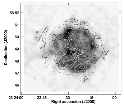
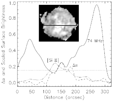
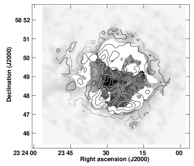
Figure 8.— Top left: $\Delta\alpha$ contours plotted over infrared [Si II] emission in greyscale at a spatial resolution of 18$\farcs$5. Positive $\Delta\alpha$ values (solid contours) indicate free-free absorption. The contour levels correspond to $\Delta\alpha$ values of: -0.05, 0.00, 0.05, 0.10, 0.15, 0.20, 0.25, and 0.30 and the signal-to-noise cutoff for the contours is 10-$\sigma$ on the 330 MHz image. Top right: Slice profiles taken at the location indicated on the inset of the $\Delta\alpha$ image. The $y$-axis indicates the value of $\Delta\alpha$ and the 74 MHz and [Si II] profiles have been scaled to show correlations between features in the images. The dotted line indicates the “average” $\Delta\alpha$ chosen for our analysis. Bottom left: Same as top left except with blanking applied to exclude shocked ejecta. Bottom right: $\Delta\alpha$ vs. [Si II] surface brightness from only unshocked ejecta. The solid line indicates the running mean of the $\Delta\alpha$ values and shows a general increase of absorption with [Si II] surface brightness.

There is not a one-to-one correlation between free-free absorption and [Si II] emission for three primary reasons. First, while the [Si II] image is a good representative of the emission observed from the unshocked ejecta in the Spitzer data, it also contains emission from shocked ejecta. As the ejecta at large radius cross the reverse shock, become heated, and contribute to the Bright Ring emission, the free-free absorption drops drastically due to the temperature dependence. We can filter the [Si II] image using the infrared [Ar II] image to blank those regions corresponding to shocked ejecta. The remaining [Si II] emission, shown in the bottom left panel of Figure 8, is dominated by unshocked ejecta and, when plotted against $\Delta\alpha$ (bottom right panel of Figure 8), shows a good correlation to the low frequency absorption. The second reason for scatter in the correlation between the free-free absorption and [Si II] emission is that the [Si II] image provides no information about other unshocked components that may be present but not detected, such as higher ionization states of Si- and O-rich ejecta or the presence of Fe-rich ejecta, for example. Finally, the $\Delta\alpha$ image is a function of both the column density of the absorbing medium and the distribution of radio emitting regions along the line of sight. The presence of clumped radio emission biases the $\Delta\alpha$ calculation to higher or lower values depending on whether the clump is on the far or near side of the unshocked ejecta in Cas A. The greater the brightness disparity between the clump and the diffuse background, the stronger the bias. We show this case in the top right panel of Figure 8 where we plot slice profiles for $\Delta\alpha$ and 74 MHz and [Si II] surface brightnesses. The peak $\Delta\alpha$ occurs at the location of a particularly bright emission clump, but has no obvious correlation to any distinct [Si II] features.

We therefore conclude that the free-free absorption is clearly correlated to the observed emission from the unshocked ejecta and is a tracer of this material as presumed by Kassim et al. (1995). Since free-free absorption depends on the temperature and density of the absorbing medium, our low frequency radio data provide a means of determining the conditions in the unshocked ejecta. When coupled with assumptions about geometry, we can also calculate the total mass of the observed unshocked ejecta. We carry out these calculations in the following sections.

5. Density and Mass of the Unshocked Ejecta

5.1. Free-Free Optical Depth

Our use of thermal absorption to probe the properties of the unshocked ejecta in Cas A relies on simplifying assumptions. Our measurement of $\Delta\alpha$, discussed above, can yield an equivalent free-free optical depth, but relies on our knowledge of the line-of-sight brightness distribution of the nonthermal, illuminating radiation from Cas A’s shell. The high spatial resolution images in Figure 2 show that Cas A consists of both clumpy and diffuse components. We assume the smooth emission has radial symmetry, consistent with shell decomposition models (Fabian et al., 1980; Gotthelf et al., 2001), so that equal contributions come from the front and back side of the shell along any line of sight. As discussed in §4, the presence of clumps will bias our measurement of $\Delta\alpha$. However, it is almost impossible to avoid clumped emission in Cas A, as Figure 2 shows. We could try using a higher frequency image to account for the clumps, but without a priori information about which clumps are in front of or behind the absorbing medium, we would introduce more uncertainties into the analysis. Therefore, we choose to select a representative absorption figure that effectively averages out the contamination from clumps. In the top right panel of Figure 8, we show the absorption profile taken along the slice indicated in the inset. The peaks and valleys of the central absorption ($\Delta\alpha$) are correlated with 74 MHz surface brightness variations, as expected. Typical $\Delta\alpha$ values in the center of Cas A range from 0.1-0.25 so we choose by eye $\Delta\alpha$=0.15 as a compromise between high and low absorption towards the center of Cas A. Since this is a somewhat arbitrary choice, we will investigate in §5.6 how the final mass and density estimates for the unshocked ejecta depend on the value of $\Delta\alpha$.

We also assume that the cold ejecta lie only in the interior of Cas A, and therefore only affect the 74 MHz emission from the back side of the shell, again consistent with three-dimensional models (DeLaney et al., 2010). We further assume the 330 MHz emission is completely unabsorbed – consistent with our spectral index measurements from 330 MHz to 5 GHz.

Based on the above picture, we derive in Appendix A the free-free optical depth $\tau$ as a function of $\Delta\alpha$:

$$\tau=-\ln[2(10^{a\Delta\alpha}-0.5)]$$ (1)

where $a=\log(74/330)$. In this formulation, spectral index is defined as $\alpha_{74}^{330}=\frac{\log(S_{74}/S_{330})}{\log(74/330)}$ and therefore is negative for a synchrotron spectrum. Using $\Delta\alpha$=0.15 results in a $\tau$ of about 0.51.

5.2. Emission Measure of the Unshocked Ejecta

The free-free absorption $\tau$ can be characterized by the following formula (Rohlfs & Wilson, 2000, chap. 9; see also Appendix B):

$$\tau_{\nu}= 3.014\times 10^{4}\left(\frac{Z^{2}}{f}\right)\left(\frac{\nu}{\mathrm{MHz}}\right)^{-2}\left(\frac{T_{e}}{\mathrm{K}}\right)^{-3/2}\left(\frac{EM}{\mathrm{pc\,cm}^{-6}}\right)$$ (2)

$$\times\ln\left[49.55Z^{-1}\left(\frac{T_{e}}{\mathrm{K}}\right)^{3/2}\left(\frac{\nu}{\mathrm{MHz}}\right)^{-1}\right]$$

where $Z$ is the average atomic number of the ions dominating the cold ejecta, $f$ is the electron to ion ratio, $\nu$ is the radio frequency in MHz at which the absorption is observed, $T_{e}$ is the temperature in K of the ionized absorbing medium, and $EM$ is the emission measure in units of pc cm^-6. Emission measure is defined as:

$$EM\equiv\int n_{e}^{2}dl$$ (3)

where $n_{e}$ is the electron density of the gas in units of cm^-3 and $dl$ is the path length along the line-of-sight measured in parsecs. Inverting Equation 2 to solve for $EM$ yields:

$$EM=\frac{3.318\times 10^{-5}\left(\frac{\tau_{\nu}f}{Z^{2}}\right)\left(\frac{\nu}{\mathrm{MHz}}\right)^{2}\left(\frac{T_{e}}{\mathrm{K}}\right)^{3/2}}{\ln\left[49.55\,Z^{-1}\left(\frac{T_{e}}{\mathrm{K}}\right)^{3/2}\left(\frac{\nu}{\mathrm{MHz}}\right)^{-1}\right]}.$$ (4)

5.3. Composition of the Absorbing Medium

To interpret $EM$, we first need to place realistic constraints on both $Z$ and $f$. Based on our observed correlation between $\Delta\alpha$ and infrared [Si II] emission, and the emission from unshocked ejecta in the infrared lines of [O IV], [S III], and [S IV] observed with Spitzer (Ennis et al., 2006; Eriksen, 2009), we assume the absorption is dominated by Si- and O-rich ejecta, including Si, S, Ar, Ca, Mg, Ne, and O. To determine the relative abundances of these species in Cas A, we rely on X-ray derived abundances indicating that the ejecta in Cas A are O-dominated (Willingale et al., 2002) and, based on stellar composition models, are typically more than a million times more abundant than hydrogen (Woosley & Weaver, 1986). Based on the abundances quoted in Willingale et al. (2002) from XMM-Newton observations of Cas A we adopt a weighted average $Z$ of 8.34.

Spectra from Spitzer and ISO (see Figure 9, Unger et al., 1997; Docenko & Sunyaev, 2010) indicate that both [O III] and [O IV] are observed from the unshocked ejecta. While models of unshocked ejecta in Cas A predict higher ionization states to be present, the material responsible for the observed infrared emission and most of the thermal absorption is in these lower ionization states (Eriksen, 2009). Therefore, we adopt an electron/ion ratio, $f$, of 2.5.

Figure 9.— ISO spectrum of the center of Cas A taken with the LWS instrument in 1996. The dotted line marks the rest wavelength of [O III]. Using the rest wavelength of 88.36 $\mu$m for [O III] results in Doppler velocities of the fitted Gaussian components as indicated. These velocities correspond to the known velocity structure of the unshocked ejecta (DeLaney et al., 2010). We note that [Fe II], with a rest wavelength of 87.38 $\mu$m, also falls into this same wavelength range, but the data are completely consistent with the [O III] origin given the known velocity structure.

At the observing frequency of 73.8 MHz, the last parameter to consider is $T_{e}$. Kassim et al. (1995) assumed, rather arbitrarily, $T_{e}$=1000 K in their calculation. A much better estimate of the temperature in the unshocked ejecta comes from the analysis of the infrared emission lines. In order to produce strong [O IV] and [Si II] lines but weak or absent [S IV] and [Ar III] lines in the Spitzer data, $T_{e}$ must be $\sim$100-500 K (Eriksen, 2009). Therefore, we will adopt $T_{e}$=300 K.

Parameterized in terms of our values for $\tau_{\nu}$, $f$, $Z$, $T_{e}$, and $\nu$, the emission measure becomes:

$$EM=\frac{17.21\left(\frac{\tau_{\nu}}{0.51}\right)\left(\frac{f}{2.5}\right)\left(\frac{Z}{8.34}\right)^{-2}\left(\frac{T_{e}}{300\,\mathrm{K}}\right)^{3/2}\left(\frac{\nu}{73.8\,\mathrm{MHz}}\right)^{2}}{\ln\left[418.3\left(\frac{T_{e}}{300\,\mathrm{K}}\right)^{3/2}\left(\frac{Z}{8.34}\right)^{-1}\left(\frac{\nu}{73.8\,\mathrm{MHz}}\right)^{-1}\right]}.$$ (5)

5.4. Geometry of Cas A

In order to estimate density from the emission measure and then estimate the total mass in the unshocked ejecta, we must assume a geometry for the absorbing medium. DeLaney et al. (2010) and Isensee et al. (2010) showed that the unshocked ejecta, as traced by [O IV] and [Si II] emission, are concentrated onto two thick sheets interior to the reverse shock – one front and one rear. The two sheets are separated by a much lower density region, where only a little emission is seen. One might expect unshocked C-rich and Fe-rich ejecta at various locations interior to the reverse shock as well based on stratification models of the ejecta (Ennis et al., 2006), however these species are not observed from the unshocked ejecta either in the Spitzer IRS spectra or the ISO LWS spectra, which could indicate that they are of lower density than the O-rich or Si-rich material, or simply absent (Eriksen, 2009).

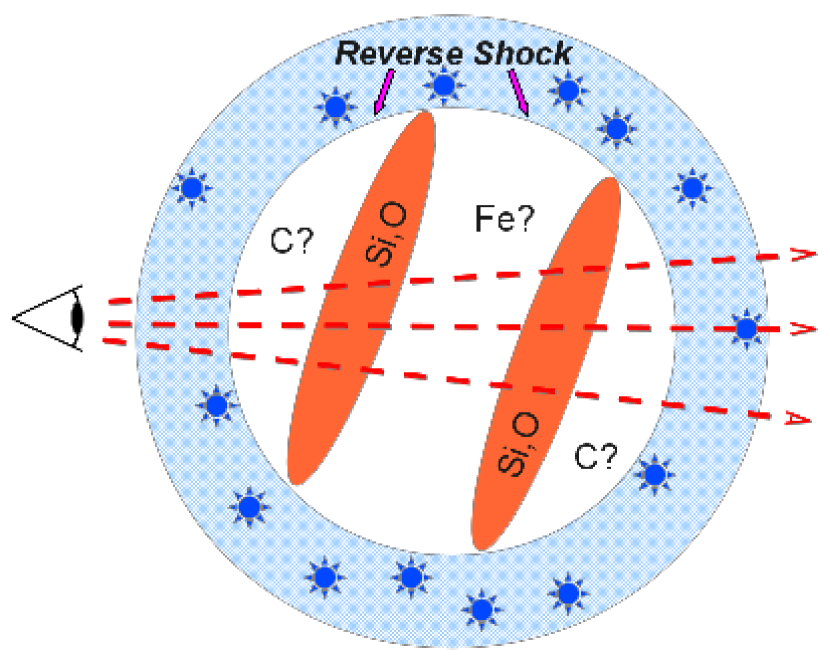
Figure 10.— Simplified drawing of the geometry of the shocked and unshocked material in Cas A. The shaded, circumferential ring represents the region bounded on its interior and exterior by the reverse shock and the blast wave, respectively. It consists of smooth (blue shaded) and clumped (blue stars) synchrotron emitting components. The two orange ellipsoids represent thermally absorbing, unshocked ejecta emitting infrared lines of Si and O. C and Fe, depicted as lying exterior and interior to the Si and O emitting material, respectively, have not been detected but might be present at lower densities.

A simplified drawing of the geometry involved is shown in Figure 10. As explained in §5.1, the emission from shocked material in Cas A can be modeled as a spherically symmetric shell consisting of smooth and clumped components. The clumpy shocked material may be ejecta, circumstellar material, or filaments associated with the forward or reverse shock. The unshocked ejecta are confined to two thick sheets in the interior. The high spectral resolution Spitzer mapping shows that the sheets are composed of thin filaments (1$\farcs$5 or 0.03 pc thick) with several filaments along any given line-of-sight (Isensee et al., 2010). Therefore, we estimate the combined thickness of the front and back sheets to be of order 10$\arcsec$ which translates to $L=$0.16 pc at the distance to Cas A of 3.4 kpc (DeLaney et al., 2010; Reed et al., 1995). The sheets intersect the reverse shock at a radius of about 90$\arcsec$ (or 1.48 pc), so that the total volume of absorbing material is $V=\pi R^{2}L=$1.1 pc³.

The geometry can be modified further by the use of a clumping factor. We know from the optical images of shocked ejecta in Cas A that there is a great deal of structure on small scales with typical knot sizes between 0$\farcs$2 and 0$\farcs$4 (Fesen et al., 2001). It is not known how much of this clumping was present prior to reverse shock passage. The effect of clumping is to reduce the total volume of material while at the same time increasing the density of the material. In order to determine the effect of clumping on our calculations, we simply modify each of our radius or thickness measures by the clumping factor ($CL$ or $CR$) so that when $C=1$ there is no clumping and when $C<1$ there is some degree of clumping. Our default value of $C$ is to assume no further clumping beyond the filamentary structures identified by Isensee et al. (2010).

5.5. Electron Density and Mass

If we assume that the density is constant, then emission measure defined in Equation 3 simplifies to $EM=n_{e}^{2}CL$ where $L$ is the combined thickness of the unshocked ejecta sheets. In Appendix C we show electron density fully parameterized in terms of $\tau_{\nu}$, $f$, $Z$, $T_{e}$, $\nu$, $C$, and $L$, however the variables in the denominator are suppressed by both a natural logarithm and a square root. Therefore we show here a simplified version of the parameterized formula in order to show how electron density depends on these various quantities:

$$n_{e}\approx 4.23\left(\frac{\tau_{\nu}}{0.51}\right)^{1/2}\left(\frac{f}{2.5}\right)^{1/2}\left(\frac{Z}{8.34}\right)^{-1}\left(\frac{T_{e}}{300\,\mathrm{K}}\right)^{3/4}$$ (6)

$$\left(\frac{\nu}{73.8\,\mathrm{MHz}}\right)C^{-1/2}\left(\frac{L}{0.16\,\mathrm{pc}}\right)^{-1/2}.$$

Thus, our estimate of electron density in the unshocked ejecta is 4.2 cm^-3.

The total mass of unshocked ejecta is simply $M=\rho V$ where $\rho$ is the mass density of the ions, $\rho=Zm_{p}n_{e}/f$, and $m_{p}$ is proton mass. If we substitute Equation C1 for $n_{e}$, assume the two thick sheet geometry, and parameterize mass in terms of $\tau_{\nu}$, $f$, $Z$, $T_{e}$, $\nu$, $C$, $R$, and $L$ then, as shown in Appendix C, the dependence on $Z$ becomes minuscule as the only surviving $Z$-term is mitigated by the natural logarithm and square root in the denominator. As we did for electron density, we show here a simplified parameterized equation for the total mass of the unshocked ejecta expressed in solar masses:

$$M\approx 0.39\left(\frac{\tau_{\nu}}{0.51}\right)^{1/2}\left(\frac{f}{2.5}\right)^{-1/2}\left(\frac{T_{e}}{300\,\mathrm{K}}\right)^{3/4}$$ (7)

$$\left(\frac{\nu}{73.8\,\mathrm{MHz}}\right)C^{5/2}\left(\frac{R}{1.48\,\mathrm{pc}}\right)^{2}\left(\frac{L}{0.16\,\mathrm{pc}}\right)^{1/2}.$$

We therefore estimate a total mass in unshocked ejecta of 0.39 M_☉ which is significantly improved compared to the 19 M_☉ estimated by Kassim et al. (1995).

5.6. Effect of Varying Parameters

We now delve into the effect our choices of $\Delta\alpha$, $C$, $T_{e}$, $f$, $Z$, and geometry have on the final electron density and mass estimates. We start with our measurement of $\Delta\alpha$ since the values are constrained by the radio observations. In Figure 11 we plot Equations C1 and C2 as functions of $\Delta\alpha$ (via $\tau$). If $\Delta\alpha$ is varied from 0.1 to 0.3, typical of the $\Delta\alpha$ values found near the middle of Cas A, the electron density and mass estimates change by a factor of two (3.3 to 6.6 cm^-3 and 0.31 to 0.62 M_☉, respectively). Even if “very strong” absorption ($\Delta\alpha$=0.4) were observed uniformly across the center of Cas A, the maximum mass estimate would still be below 1 M_☉.

Also shown in Figure 11 are Equations C1 and C2 plotted as functions of clumping. Recall that $C=1$ indicates no clumping, while smaller values of $C$ increase the amount of clumping in the ejecta. As clumping increases, the electron density increases and the total mass estimate decreases. For all modest clumping estimates, the electron density remains below 10 cm^-3 and the total mass remains below 1 M_☉.

Figure 11.— Plots of Equation C1 (top) and Equation C2 (bottom) as functions of $\Delta\alpha$ (via $\tau$) and clumping factor. For each curve, one of the variables are held constant as indicated. Each of the $x$-axes is independent with $\Delta\alpha$ indicated on the bottom $x$-axis and clumping ($C$) indicated on the top $x$-axis in each plot.

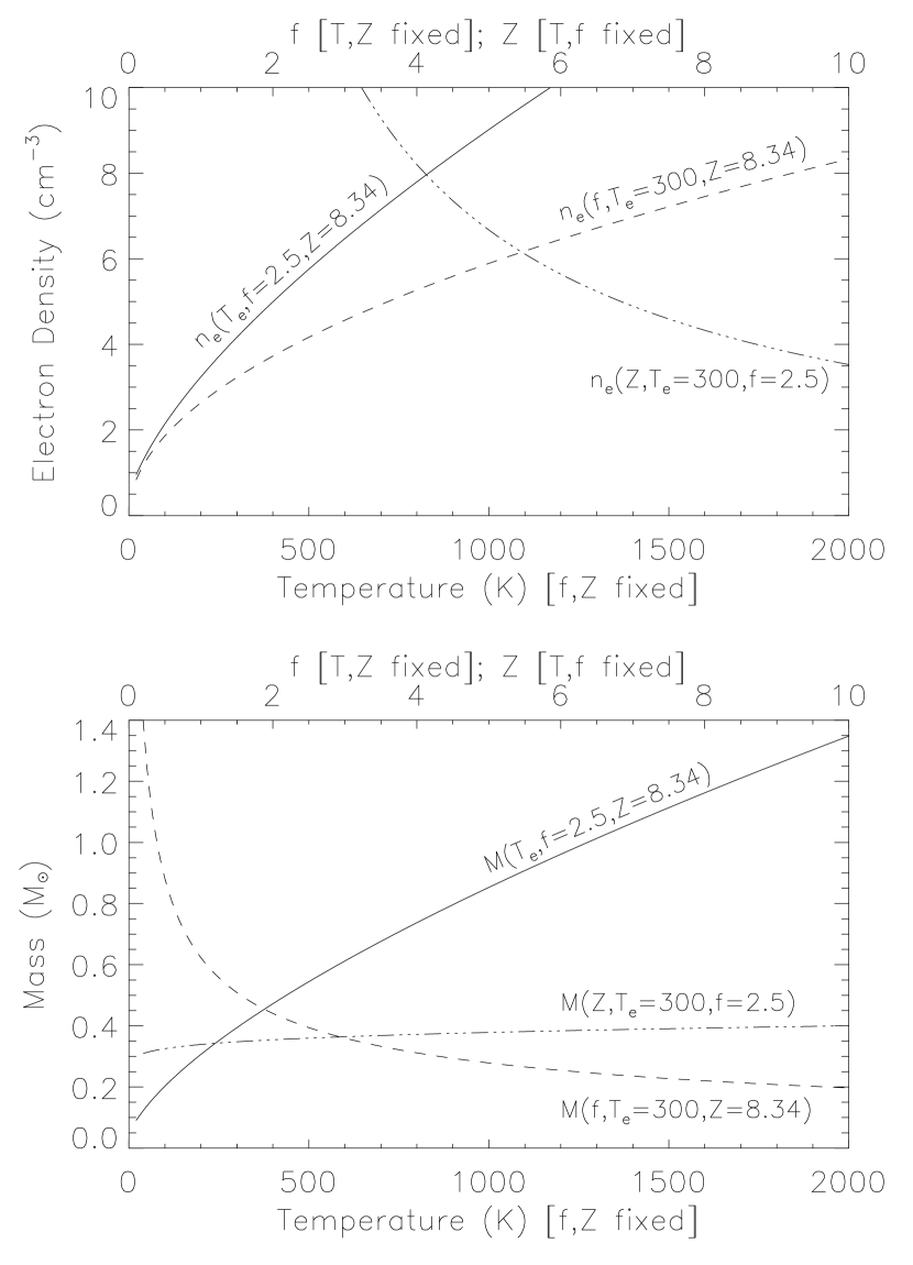
Figure 12.— Plots of Equation C1 (top) and Equation C2 (bottom) as functions of $T_{e}$, $f$, and $Z$. For each curve, two of the variables are held constant as indicated. Each of the $x$-axes is independent with temperature indicated on the bottom $x$-axis and atomic number ($Z$) and electron/ion ratio ($f$) indicated on the top $x$-axis in each plot.

The values of $T_{e}$, $f$, and $Z$ depend on emission models and observations that may be affected by components that are missing because we have no probe for them, such as higher ionization states of Si (Eriksen, 2009). To illustrate the effect of varying these quantities, we plot Equations C1 and C2 in Figure 12. For each of the plotted curves, two of the values are held constant as indicated. All reasonable estimates of $T_{e}$, $f$, and $Z$ require that the electron density be less than 10 cm^-3. While the total unshocked ejecta mass is much more strongly influenced by temperature and electron/ion ratio than atomic number, plausible variations in all three variables constrain the mass below 1 M_☉.

The final effect we would like to address is that of the geometry. While the two thick sheet geometry for the unshocked ejecta is supported by the morphology of the infrared [Si II] and [O IV] emission, and the correlation between the $\Delta\alpha$ map and [Si II] is quite good, this is not a one-to-one correlation. Other species possibly in different locations along the line-of-sight might be responsible for some of the observed thermal absorption. Therefore, we consider here a spherical geometry in which the unshocked ejecta are modeled as a filled sphere of absorbing material interior to the bright radio-emitting ring. Since the emission measure derives from the $\Delta\alpha$ measurement, it does not change, however the path length through the absorbing medium does. If we use $L=2.96$ pc through the center of Cas A so that $R=L/2=1.48$ pc as before, and we assume that $n_{e}$ is constant, then the electron density from Equations 6 and C1 becomes 0.98 cm^-3 and the total mass of the unshocked ejecta becomes 1.12 M_☉ as derived in Equation C3. A clumping factor would increase the electron density and decrease the total mass estimate.

6. Discussion

6.1. Improvement over Previous Mass Estimate

As mentioned previously, Kassim et al. (1995) estimated a total mass of 19 M_☉ for the unshocked ejecta. The dominant reason for this high mass value is that the free-free optical depth equation used by Kassim et al. (1995) was for a hydrogenic gas, rather than an oxygenic gas, as appropriate for a core-collapse SNR. In addition, Kassim et al. (1995) made a number of assumptions about other model parameters that significantly affected their final mass values. Specifically, their temperature was 1000 K compared to our value of 300 K. They used their maximum $\Delta\alpha$ of 0.3 compared to our more modest estimate of 0.15. They correctly assumed the ejecta were dominated by oxygen, but incorrectly assumed that the oxygen was singly ionized. Kassim et al. (1995) also assumed a spherical ejecta distribution rather than our two-thick-sheet morphology. Thus, the confluence of parameter values chosen, and using an incorrect formula for free-free optical depth, resulted in a very high mass estimate in the earlier work.

6.2. Comparison with Theoretical Expectations for Density and Mass

The density and temperature conditions in the unshocked ejecta and the total mass of this material play a key role in many aspects of supernova remnant physics. Laming & Hwang (2003) and Hwang & Laming (2003, 2012) have incorporated results from their analysis of the million-second observation of Cas A with Chandra into hydrodynamic simulations of supernova remnant evolution that account for factors such as expansion into a stellar wind and acceleration of the reverse shock. Their models, designed to match the dynamics of Cas A, result in a range of total and shocked ejecta masses, which are then partitioned into the various elemental species based on their derived abundances from the X-ray data. Their most recent prediction for the total mass of ejecta that are currently unshocked is 0.18-0.3 M_☉, depending on the model chosen. Which species dominate the composition of the unshocked ejecta is debatable since the explosion is known to have been asymmetric (Rest et al., 2011). Hwang & Laming (2012) argue that there is little Fe left in the unshocked ejecta based on several factors including the lack of infrared Fe emission from the unshocked ejecta (Smith et al., 2009), the location of the X-ray-emitting Fe-rich ejecta at the same or larger radius than the Si-rich ejecta (Hughes et al., 2000) and the carbon atmosphere of the neutron star (Ho & Heinke, 2009). Our estimate of 0.39 M_☉ for the unshocked ejecta is near the upper limit predicted by Hwang & Laming (2012), however reasonable variations of our parameters, such as increasing the clumping factor, can lead to lower values of total unshocked ejecta mass in line with the prediction.

We can also compare the density of the unshocked ejecta to the hydrodynamic model of Hwang & Laming (2012). Their ejecta model assumes a uniform density core surrounded by a power-law envelope. The density of the core as a function of time is given by:

$$\rho_{\mathrm{core}}=\left(\frac{M_{ej}}{v_{\mathrm{core}}^{3}}\right)\left(\frac{3}{4\pi}\right)\left(\frac{n-3}{n}\right)t^{-3}$$ (8)

where $M_{ej}$ is the total mass of the ejecta and the factor $(n-3)/n$ gives the fraction of the ejecta mass in the core (Laming & Hwang, 2003; Hwang & Laming, 2012; Truelove & McKee, 1999). $v_{\mathrm{core}}$ is the velocity of the boundary between the core and the power-law envelope. For an $n=10$ power-law envelope and $M_{ej}=$3 M_☉, Hwang & Laming (2012) report $v_{\mathrm{core}}\approx 9000$ km s^-1. At an age of 330 years, $\rho_{\mathrm{core}}\approx 1\times 10^{-24}$ g cm^-3. Our “filled sphere” geometry provides a convenient comparison because it, too, assumes a uniform density ejecta distribution throughout the interior of the SNR with no clumping. For $n_{e}=0.98$ cm^-3, $f$=2.5, and $Z$=8.34, we derive $\rho_{\mathrm{sph}}=5.5\times 10^{-24}$ g cm^-3, which is only a factor of 5 larger than Hwang & Laming (2012).

The ejecta in Cas A are distributed in a complex fashion and the unshocked ejecta show signs of filamentary behavior in the high spectral resolution Spitzer data (Isensee et al., 2010). For any given emission measure, if the material is tied up in clumps, the final density estimate will be higher and the final mass estimate would be lower than when the material is distributed uniformly along the line-of-sight. In order to match our mass estimate with that of Hwang & Laming (2012), this would argue for the unshocked ejecta being primarily distributed in the two-shell geometry. Any unshocked C-rich or Fe-rich ejecta must then be of such low density that it makes little contribution to the observed thermal absorption – or one or both of these components are missing entirely.

Our calculations favor a low density and low temperature environment in the unshocked ejecta consistent with the analysis of the Spitzer infrared data (Eriksen, 2009). Temperatures $\lesssim$500 K are not unexpected given the rapid expansion of the SNR, which could conceivably cool the ejecta to $\sim$10s of Kelvin, and the fact that the infrared flux densities infer unshocked dust temperatures of about 35 K (see e.g. Nozawa et al., 2010). Expectations for the density of the unshocked ejecta are not clear. While hydrodynamic models can predict an average density, as in Equation 8, the clumping of the ejecta renders the average somewhat meaningless. If the unshocked ejecta we detect via thermal absorption and mid-infrared emission eventually radiate strongly in the X-rays upon shock heating, then our density estimate is in line with that expectation. The electron densities observed in the X-ray-emitting (shocked) ejecta are $\sim$10s cm^-3 which would be consistent with the standard strong shock compression ratio of 4. On the other hand, much more dense (1000s cm^-3) shocked ejecta are observed optically (see e.g. Chevalier & Kirshner, 1979) indicating that the unshocked ejecta must have a much denser, clumped component in order to reproduce the observed range of shocked ejecta densities (Morse et al., 2004). A high degree of clumping might arise due to the instabilities associated with the explosion reverse shock which forms inside of the star in the first few hours after the explosion begins (Herant & Woosley, 1994; Joggerst, Woosley, & Heger, 2009). Similarly, turbulence and strong clumping are associated with expanding Fe-Ni bubbles in the inner ejecta (Li, McCray, & Sunyaev, 1993; Blondin, Borkowski, & Reynolds, 2001). The expansion of Fe-Ni bubbles naturally renders the innermost Fe ejecta of very low density, consistent with the lack of detected infrared Fe emission in the unshocked ejecta.

6.3. Comparison to SN1006

The only other confirmed detection of unshocked ejecta in an SNR is that of SN1006 where high-velocity absorption features were observed in ultraviolet lines of Fe II and Si II (Wu et al., 1983; Hamilton et al., 1997). High resolution spectra showed no detectable unshocked Si III or Si IV and thus the bulk of the unshocked Si is accounted for with Si II absorption (Winkler et al., 2005; Hamilton, Fesen, & Blair, 2007). The total Si mass calculated from the derived column densities (0.25 M_☉) is roughly comparable with the Si mass predicted from some white dwarf carbon deflagration models (0.16 M_☉) and the derived Si mass from X-ray data (0.2 M_☉) (Hamilton et al., 1997).

Accounting for the unshocked Fe in SN1006 has proven to be more difficult. Hamilton et al. (1997) argue that the unshocked Fe absorption should be dominated by Fe II because the photoionization cross section is five times that of Si II. However, the total mass in Fe II (0.029 M_☉) is less than 1/10 of that expected from carbon deflagration models (0.3 M_☉) (Hamilton & Fesen, 1988; Hamilton et al., 1997). The absence of Fe II absorption along some lines-of-sight indicate that there is likely no large-scale mixing or overturning of Fe ejecta, so the bulk of the Fe must still be interior to the reverse shock (Winkler et al., 2005). There is the possibility that the Fe is tied up in higher ionization states (Hamilton & Fesen, 1988), but then the lack of Si III and Si IV absorption from the unshocked ejecta is puzzling (Hamilton et al., 1997). Therefore, it seems that some of the unshocked ejecta in SN1006 are still unaccounted for.

In Cas A, there is a similar “problem” between the strong emission from [Si II] and the lack of any detectable infrared Fe emission from the unshocked ejecta in the Spitzer IRS bands or the ISO LWS spectra. At the density we infer for the unshocked ejecta, [Si II] should be much stronger than [Fe II] and [Fe III], however [Fe V] should be comparable to the [Si II] (Eriksen, 2009), which is not observed (Smith et al., 2009). As explained in §6.2, the Fe discrepancy in Cas A may be resolved if the bulk of the Fe ejecta have already passed through the reverse shock and the remaining interior Fe is of lower density than the unshocked Si- and O-rich ejecta. However, we need a better knowledge of Cas A’s progenitor and the expected Fe yields for a Type IIb explosion of such a star in order to determine if all of the Fe ejecta in Cas A are truly accounted for.

One other comparison we can make to SN1006 is of the density in the unshocked ejecta. Hamilton et al. (1997) estimate $\rho_{\mathrm{FeII}}\sim 4\times 10^{-27}$ g cm^-3 at the center of their unshocked ejecta profile with an estimate of about half that figure for the current unshocked mass density of Si II. If we scale the mass density of the (O-rich) unshocked ejecta in Cas A by 27 to account for the difference in age of the two SNRs and thus the dilution of the density due to expansion, then $\rho_{\mathrm{sph}}^{1000}=2\times 10^{-25}$ g cm^-3. Therefore the observed unshocked ejecta in Cas A are about 100 times more dense than in SN1006. Given that Cas A is the result of a Type IIb explosion and SN1006 resulted from a Type Ia explosion, stark differences in ejecta density are to be expected due to differing stellar compositions, explosion mechanisms and resulting nucleosynthesis, initial ejecta density profiles, instabilities in the ejecta that may lead to clumping, and circumstellar environments. The question is are the unshocked ejecta in Type Ia SNRs systematically less dense than in core-collapse remnants? The extension of low frequency radio analysis to other SNRs could be used to test this hypothesis. Furthermore, since the absorption is frequency dependent, working at frequencies lower than 74 MHz will allow the detection of lower density ejecta in Cas A and other SNRs.

6.4. Implications for Lower Frequency Spectrum

Helmboldt & Kassim (2009) revisited the low frequency, integrated spectrum of Cas A utilizing legacy VLA and Long Wavelength Development Array 74 MHz measurements. We consider here how the thermal absorption discussed in this paper relates to the turnover in the integrated spectrum of Cas A at much lower frequencies, as originally documented by Baars et al. (1977). Given the current limited angular resolution of observations towards Cas A below 74 MHz, our discussion is necessarily limited.

Examination of the Baars et al. (1977) Figure 1a indicates the integrated spectrum of Cas A begins to turn over below 38 MHz. The Baars et al. (1977) modeled spectrum (epoch 1965) which did not fit for a turnover, predicts $\sim$93,000 Jy at 10 MHz. The lowest reliable flux density measurement at that frequency is the Penticton 10 MHz flux density of 28,000 Jy (epoch 1965.9, i.e. contemporaneous, Bridle 1967), which is a factor of 3.3 below the expected value. (This corresponds to a 10 MHz free-free optical depth by a uniform external absorber of $\sim$1.2, an oversimplification since some of the absorption must be internal.) As described in Section 5.1, an average free-free optical depth for the unshocked ejecta at 74 MHz is $\sim$0.5, which rapidly inflates to $\gg$1 at 10 MHz, i.e. completely opaque. If the absorbing ejecta blocked $\sim$30% of the back surface of Cas A’s nonthermal emission, $\sim$85% of Cas A’s 10 MHz emission, or $\sim$79,000 Jy, should escape the remnant. We can account for the remaining deficit by an intervening thermal absorber with $\tau_{10\,\mathrm{MHz}}\sim-\ln(28,000/79,000)\sim 1$. Thus, a simplistic scenario has $\sim$79,000 Jy of Cas A’s 10 MHz emission emerging from the remnant after being attenuated by $\sim$15% from the unshocked ejecta. Thereafter the emerging emission is further attenuated by an intervening ionized component of the ISM with 10 MHz optical depth $\sim$1.

The distribution of low density gas in the interstellar medium was constrained by Kassim (1989), using the observed, patchy thermal absorption inferred from the low frequency, integrated spectra of Galactic SNRs. (Several of those systems have since been resolved with legacy VLA data (Lacey et al., 2001; Brogan et al., 2005).) The measured optical depths at 30.9 MHz typically ranged from 0.1-1, though some remnants showed no turnovers while others were more heavily absorbed. The nature of the absorption was consistent with higher frequency recombination line observations that postulated extended H II region envelopes (EHEs) associated with normal H II regions (Anantharamaiah, 1986). The inferred ISM 10 MHz free-free optical depth unity discussed above, and required to further attenuate Cas A’s emerging emission, scales to $\sim$0.1 at 30.9 MHz. Thus the low frequency turnover in the integrated spectrum of Cas A is qualitatively consistent with a combination of intrinsic absorption from unshocked ejecta and extrinsic absorption by EHEs located along the line of sight. In retrospect the Baars et al. (1977) low frequency turnover would be conspicuous in its absence based on what we now know about ionized gas in both the ISM and Cas A.

7. Future Work

The radio detection of thermally absorbing, unshocked ejecta inside a young Galactic SNR by the legacy VLA 74 MHz system only scratches the surface of possibilities for emerging low frequency systems with greater capabilities. With the transition to the fully digital electronics and new correlator of the VLA, the narrowband 74 and 330 MHz legacy systems have been replaced with an improved, broad-band “Low Band” receiving system (Clarke et al., 2011). The new, single receiver system brings significant improvements over its two narrow band predecessors, and will become available to the VLA user community in 2014.

For broad band systems probing below 74 MHz, e.g. LOFAR Low Band (van Haarlem et al., 2013), or LWA, the frequency dependence of thermal absorption significantly enhances the effect. Gradually tuning to lower frequencies as the absorption grows can break the optical depth degeneracy between temperature and emission measure, and deconvolve the radial superposition of nonthermal emitting and thermal absorbing regions. Lower frequency observations with sufficient angular resolution (e.g. LOFAR Low Band) can test our qualitative assessment of the relative contributions of intrinsic and extrinsic thermal absorption contributing to the observed turnover in Cas A’s integrated spectrum below 38 MHz. It is also important to constrain the emission at frequencies above 74 MHz just prior to the onset of absorption, as offered e.g. by LOFAR High Band, MWA, the GMRT, and VLA Low Band.

Helmboldt & Kassim (2009) also confirmed shorter scale (5-10 yr) temporal variations at 74 MHz consistent with previous reports in the literature for low frequencies (Erickson & Perley, 1975; Vinyaĭkin & Razin, 2005). These have generally been attributed to the interaction of the forward shock with an inhomogeneous CSM or ISM. However some variation must also arise from inside Cas A, as the reverse shock advances into the unshocked ejecta and affects its opacity. Together with the secular decrease due to adiabatic expansion (Shklovskii, 1960), the overall temporal behavior is necessarily complex, and requires higher resolution, broad band low frequency measurements to understand. We suggest that Cas A’s low frequency flux density should be monitored routinely across a range of lower frequencies; for instruments such as LOFAR or LWA this would require only a few minutes of observations every few weeks or months and would allow a much better determination of the range of timescales over which such variations occur.

8. Conclusions

We have imaged Cas A from 5 GHz to 74 MHz in all four configurations of the Legacy VLA with follow-up observations at 74 and 330 MHz with the legacy VLA+PT link. Our spatially resolved spectral index maps confirm the interior spectral flattening measured earlier, but at higher signal-to-noise and resolution. Comparison with Spitzer infrared spectra confirms the earlier hypothesis that the spectral flattening is due to thermal absorption by cool, unshocked ejecta photoionized by X-ray radiation from Cas A’s reverse shock. We use the spectral flattening to measure the free-free optical depth.

Next, using priors of electron temperature, atomic number, and electron to ion ratios, we derive an emission measure from the measured optical depth. With an assumed geometry, informed from three-dimensional modeling based on higher frequency studies, we use the emission measure to place constraints on both the density and total mass of the unshocked ejecta.

We consider modest, physically plausible variations in both our priors and the assumed geometry, and find that the effect on the total mass is relatively modest, varying by a factor of about two. Furthermore, our derived total mass is consistent with recent model predictions (Hwang & Laming, 2012). After accounting for the relative ages of Cas A and SN1006, our derived mass density is much higher than found in SN1006, not unexpected since Cas A (Type IIb) and SN1006 (Type Ia) emerged from two fundamentally different supernova explosion types. However, if there is a systematic difference in unshocked ejecta density for core collapse vs. Type Ia SNRs, low frequency radio data can be used to test this hypothesis.

Finally, we consider the contribution of the intrinsic thermal absorption to the known turnover of Cas A’s integrated spectrum at much lower frequencies. We find that the intrinsic thermal absorption from the unshocked ejecta, combined with extrinsic absorption from a known, patchy distribution of low density ISM gas, are completely consistent with the low frequency turnover.

The promise of the emerging instruments is expanding the population of SNRs, young and old, that can be probed for intrinsic and extrinsic thermal absorption and shock acceleration variations beyond pathologically bright sources like Cas A. More generally, the seemingly ubiquitous detection of resolved thermal absorption by the 74 MHz legacy VLA against the Galactic background (Nord et al., 2006) and towards, discrete non thermal sources (e.g. see Lacey et al., 2001; Brogan et al., 2005; Castelletti et al., 2007) confirms the phenomena will continue to emerge as a powerful tool for low frequency astrophysics.

Appendix A Derivation of $\tau-\Delta\alpha$ Relation

The definition of spectral index between 74 and 330 MHz is

$$\alpha_{74}^{330}=\frac{\log(S_{74}/S_{330})}{\log(74/330)},$$ (A1)

where $\alpha$ is negative for nonthermal emission. We also define $a=\log\left(\frac{74}{330}\right)$.

Assuming no curvature in the emitted synchrotron spectrum, we expect ($e$) the spatially resolved spectral index $\alpha$ to remain unchanged from above 330 MHz to between 330 and 74 MHz, defining $\alpha_{e}$. $\alpha_{o}$ is then defined as the observed ($o$) spectral index due to absorption.

The difference between observed and expected spectral index is then: $\Delta\alpha=\alpha_{o}-\alpha_{e}$ ($\Delta\alpha$ is positive), so that:

$$\Delta\alpha=\frac{\log(S_{o74}/S_{330})-\log(S_{e74}/S_{330})}{a}=\frac{\log(S_{o74}/S_{e74})}{a}$$ (A2)

To obtain observed and expected 74 MHz flux density, we assume equal synchrotron emission from the front and back sides ($S_{f}=S_{b}$) of Cas A:

$$S_{e}=S_{f}+S_{b}=2S_{f}$$ (A3)

$$S_{o}=S_{f}+S_{f}e^{-\tau}=(1+e^{-\tau})S_{f}$$ (A4)

$$\frac{S_{o}}{S_{e}}=\frac{1+e^{-\tau}}{2}$$ (A5)

Substituting for $\frac{S_{o}}{S_{e}}$ we have:

$$a\Delta\alpha=\log\left(\frac{S_{o74}}{S_{e74}}\right)=\log\left(\frac{1+e^{-\tau}}{2}\right)$$ (A6)

$$2(10^{a\Delta\alpha})=1+e^{-\tau}$$ (A7)

$$\tau=-\ln[2(10^{a\Delta\alpha}-0.5)]$$ (A8)

We note that Equation A8 is slightly different than that published in Kassim et al. (1995) due to a typographical error.

Appendix B Calculation of Free-Free Optical Depth $\tau$

In this section, we follow the derivation in chapter 9 of Rohlfs & Wilson (2000).

The definition of free-free optical depth ($\tau$) is:

$$\tau_{\nu}=-\int\kappa_{\nu}dl$$ (B1)

where

$$\kappa_{\nu}=\frac{4Z^{2}e^{6}}{3c}\frac{n_{i}n_{e}}{\nu^{2}}\frac{1}{\sqrt{2\pi(mkT_{e})^{3}}}\left<g_{ff}\right>$$ (B2)

is the absorption coefficient and the Gaunt factor is

$$\left<g_{ff}\right>=\ln\left[\left(\frac{2kT_{e}}{\gamma m_{e}}\right)^{3/2}\frac{m_{e}}{\pi\gamma Ze^{2}\nu}\right].$$ (B3)

$Ze$ is the ion charge, $n_{i}$ and $n_{e}$ are number density of ions and electrons, respectively. $c$ is the speed of light, $\nu$ is the observation frequency, $m_{e}$ is the electron mass, $k$ is Boltzmann’s constant, $\gamma=1.781$, and $T_{e}$ is the effective temperature of the gas which must be $>20$ K.

For classic H II regions one normally assumes a hydrogenic gas where $Z=1$ and $n_{e}=n_{i}$, but that is not the case here (Woosley & Weaver, 1986). Let $f=n_{e}/n_{i}$ and use emission measure $=EM\equiv\int n_{e}^{2}\,dl$ and express $T_{e}$ in K, $\nu$ in MHz, and $EM$ in pc cm^-6 so that:

$$\tau_{\nu}=3.014\times 10^{4}\left(\frac{Z^{2}}{f}\right)\left(\frac{\nu}{\mathrm{MHz}}\right)^{-2}\left(\frac{T_{e}}{\mathrm{K}}\right)^{-3/2}\left(\frac{EM}{\mathrm{pc\,cm}^{-6}}\right)\ln\left[49.55Z^{-1}\left(\frac{T_{e}}{\mathrm{K}}\right)^{3/2}\left(\frac{\nu}{\mathrm{MHz}}\right)^{-1}\right].$$ (B4)

Appendix C Full Parameterized Equations for Electron Density and Total Mass

The electron density follows from Equation 3 and our preferred geometry as $n_{e}=\sqrt{EM/CL}$. Substituting Equation 5 into this expression yields:

$$n_{e}=\frac{10.4\left(\frac{\tau_{\nu}}{0.51}\right)^{1/2}\left(\frac{f}{2.5}\right)^{1/2}\left(\frac{Z}{8.34}\right)^{-1}\left(\frac{T_{e}}{300\,\mathrm{K}}\right)^{3/4}\left(\frac{\nu}{73.8\,\mathrm{MHz}}\right)C^{-1/2}\left(\frac{L}{0.16\,\mathrm{pc}}\right)^{-1/2}}{\left\{\ln\left[418.3\left(\frac{T_{e}}{300\,\mathrm{K}}\right)^{3/2}\left(\frac{Z}{8.34}\right)^{-1}\left(\frac{\nu}{73.8\,\mathrm{MHz}}\right)^{-1}\right]\right\}^{1/2}}$$ (C1)

where $n_{e}$ is in units of cm^-3.

The total mass in unshocked ejecta is calculated from $M=(Zm_{p}n_{e}/f)(\pi C^{3}R^{2}L)$, where $m_{p}$ is proton mass. Substituting Equation C1 for $n_{e}$ and absorbing constant terms results in the following equation for total mass in solar masses:

$$M=\frac{0.97\left(\frac{\tau_{\nu}}{0.51}\right)^{1/2}\left(\frac{f}{2.5}\right)^{-1/2}\left(\frac{T_{e}}{300\,\mathrm{K}}\right)^{3/4}\left(\frac{\nu}{73.8\,\mathrm{MHz}}\right)C^{5/2}\left(\frac{R}{1.48\,\mathrm{pc}}\right)^{2}\left(\frac{L}{0.16\,\mathrm{pc}}\right)^{1/2}}{\left\{\ln\left[418.3\left(\frac{T_{e}}{300\,\mathrm{K}}\right)^{3/2}\left(\frac{Z}{8.34}\right)^{-1}\left(\frac{\nu}{73.8\,\mathrm{MHz}}\right)^{-1}\right]\right\}^{1/2}}.$$ (C2)

If a spherical geometry is assumed, then $M=(Zm_{p}n_{e}/f)(\frac{4}{3}\pi C^{3}R^{3})$ which becomes:

$$M=\frac{2.73\left(\frac{\tau_{\nu}}{0.51}\right)^{1/2}\left(\frac{f}{2.5}\right)^{-1/2}\left(\frac{T_{e}}{300\,\mathrm{K}}\right)^{3/4}\left(\frac{\nu}{73.8\,\mathrm{MHz}}\right)C^{5/2}\left(\frac{R}{1.48\,\mathrm{pc}}\right)^{3}\left(\frac{L}{2.96\,\mathrm{pc}}\right)^{-1/2}}{\left\{\ln\left[418.3\left(\frac{T_{e}}{300\,\mathrm{K}}\right)^{3/2}\left(\frac{Z}{8.34}\right)^{-1}\left(\frac{\nu}{73.8\,\mathrm{MHz}}\right)^{-1}\right]\right\}^{1/2}}.$$ (C3)

References

- Anantharamaiah (1986) Anantharamaiah, K. R. 1986, JApA, 7, 131
- Anderson et al. (1991) Anderson, M., Rudnick, L., Leppik, P., Perley, R., & Braun, R. 1991, ApJ, 373, 146
- Anderson & Rudnick (1995) Anderson, M. & Rudnick, L. 1995, ApJ, 441, 307
- Baars et al. (1977) Baars, J. W. M., Genzel, R., Pauliny-Toth, I. I. K., & Witzel, A. 1977, A&A, 61, 99
- Blondin, Borkowski, & Reynolds (2001) Blondin, J. M., Borkowski, K. J., & Reynolds, S. P. 2001, ApJ, 557, 782
- Bridle (1967) Bridle, A. H. 1967, The Observatory, 87, 60
- Brogan et al. (2005) Brogan, C. L., Lazio, T. J., Kassim, N. E., & Dyer, K. K. 2005, AJ, 130, 148
- Castelletti et al. (2007) Castelletti, G., Dubner, G., Brogan, C., & Kassim, N. E. 2007, A&A, 471, 537
- Chevalier & Kirshner (1979) Chevalier, R. & Kirshner, R. P. 1979, ApJ, 233, 154
- Clarke et al. (2011) Clarke, T. E., Kassim, N. E., Hicks, B. C., Owen, F. N., Durand, S., Kutz, C., Pospieszalski, M., Perley, R. A., Weiler, K. W., Wilson, T. L. 2011, Memorie della Societa Astronomica Italiana, 82, 664
- DeLaney et al. (2010) DeLaney, T., Rudnick, L., Stage, M. D., Smith, J. D., Isensee, K., Rho, J., Allen, G. E., Gomez, H., Kozasa, T., Reach, W. T., Davis, J. E., & Houck, J. C. 2010, ApJ, 725, 2038
- Docenko & Sunyaev (2010) Docenko, D., & Sunyaev, R. A. 2010, A&A, 509, A59
- Ennis et al. (2006) Ennis, J. A., Rudnick, L., Reach, W. T., Smith, J. D., Rho, J., DeLaney, T., Gomez, H., & Kozasa, T. 2006, ApJ, 652, 376
- Eriksen (2009) Eriksen, K. A. 2009, PhD dissertation, Univ. Arizona
- Erickson & Perley (1975) Erickson, W. C. & Perley, R. A. 1975, ApJ, 200, L83
- Fabian et al. (1980) Fabian, A. C., Willingale, R., Pye, J. P., Murray, S. S., & Fabbiano, G. 1980, MNRAS, 193, 175
- Fesen et al. (2001) Fesen, R. A., Morse, J. A., Chevalier, R. A., Borkowski, K. J., Gerardy, C. L., Lawrence, S. S., & van den Bergh, S. 2001, ApJ, 122, 2644
- Gotthelf et al. (2001) Gotthelf, E. V., Koralesky, B., Rudnick, L., Jones, T. W., Hwang, U., & Petre, R. 2001, ApJ, 552, L39
- Hamilton & Fesen (1988) Hamilton, A. J. S. & Fesen, R. A. 1988, ApJ, 327, 178
- Hamilton et al. (1997) Hamilton, A. J. S., Fesen, R. A., Wu, C.-C., Crenshaw, D. M., & Sarazin, C. L. 1997, ApJ, 481, 838
- Hamilton, Fesen, & Blair (2007) Hamilton, A. J. S., Fesen, R. A., & Blair, W. P. 2007, MNRAS, 381, 771
- Hammell & Fesen (2008) Hammell, M. C., & Fesen, R. A. 2008, ApJS, 179, 195
- Helmboldt & Kassim (2009) Helmboldt, J. F. & Kassim, N. E. 2009, AJ, 138, 838
- Herant & Woosley (1994) Herant, M. & Woosley, S. E. 1994, ApJ, 425, 814
- Ho & Heinke (2009) Ho, W. C. G. & Heinke, C. O. 2009, Nature, 462, 71
- Hughes et al. (2000) Hughes, John P., Rakowski, Cara E., Burrows, David N., & Slane, Patrick O. 2000, ApJ, 528, L109
- Hwang & Laming (2003) Hwang, U. & Laming, J. M. 2003, ApJ, 597, 362
- Hwang & Laming (2012) Hwang, U. & Laming, J. M. 2012, ApJ, 746, 130
- Isensee et al. (2010) Isensee, Karl, Rudnick, Lawrence, DeLaney, Tracey, Smith, J. D., Rho, Jeonghee, Reach, William T., Kozasa, Takashi, & Gomez, Haley 2010, ApJ, 725, 2059
- Joggerst, Woosley, & Heger (2009) Joggerst, C. C., Woosley, S. E., & Heger, A. 2009, ApJ, 693, 1780
- Kassim et al. (2007) Kassim, N. E., Lazio, T. J. W., Erickson, W. C., Perley, R. A., Cotton, W. D., Greisen, E. W., Cohen, A. S., Hicks, B., Schmitt, H. R., & Katz, D. 2007, ApJS, 172, 686
- Kassim et al. (1995) Kassim, N. E., Perley, R. A., Dwarakanath, K. S., Erickson, W. C. 1995, ApJ, 455, L59
- Kassim et al. (1993) Kassim, N. E., Perley, R. A., Erickson, W. C., & Dwarakanath, K. S. 1993, AJ, 106, 2218
- Kassim (1989) Kassim, N. E. 1989, ApJ, 347, 915
- Krause et al. (2008) Krause, O., Birkmann, S. M., Usuda, T., Hattori, T., Goto, M., Rieke, G. H., & Misselt, K. A. 2008, Science, 320, 1195
- Lacey et al. (2001) Lacey, C. K., Lazio, T. J. W., Kassim, N. E., Duric, N., Briggs, D. S., & Dyer, K. K. 2001, ApJ, 559, 954
- Laming & Hwang (2003) Laming, J. M. & Hwang, U. 2003, ApJ, 597, 347
- Li, McCray, & Sunyaev (1993) Li, H., McCray, R., & Sunyaev, R. A. 1993, ApJ, 419, 824
- Morse et al. (2004) Morse, Jon A., Fesen, Robert A., Chevalier, Roger A., Borkowski, Kazimierz J., Gerardy, Christopher L., Lawrence, Stephen S., & van den Bergh, Sidney 2004, ApJ, 614, 727
- Nord et al. (2006) Nord, M.E., Henning, P.A., Rand, R.J., Lazio, T.J.W., & Kassim 2006, N. E., AJ, 132, 242
- Nozawa et al. (2010) Nozawa, T., Kozasa, T., Tominaga, N., Maeda, K., Umeda, H., Nomoto, K.,& Krause, O. 2010, ApJ, 713, 356
- Perley & Taylor (1991) Perley, R. A. & Taylor, G. B. 1991, AJ, 101, 1623
- Reed et al. (1995) Reed, J. E., Hester, J. J., Fabian, A. C., & Winkler, P. F. 1995, ApJ, 440, 706
- Rees (1990) Rees, N. 1990, MNRAS, 243, 637
- Rest et al. (2011) Rest, A., Foley, R. J., Sinnott, B., Welch, D. L., Badenes, C., Filippenko, A. V., Bergmann, M., Bhatti, W. A., Blondin, S., Challis, P., Damke, G., Finley, H., Huber, M. E., Kasen, D., Kirshner, R. P., Matheson, T., Mazzali, P., Minniti, D., Nakajima, R., Narayan, G., Olsen, K., Sauer, D., Smith, R. C., & Suntzeff, N. B. 2011, ApJ, 732, 3
- Rohlfs & Wilson (2000) Rohlfs K. & Wilson, T. L. 2000, Tools of Radio Astronomy, (3rd ed., Berlin:Springer-Verlag)
- Ryle, Elsmore, & Neville (1965) Ryle, M., Elsmore, B., & Neville, A. C. 1965, Nature, 205, 1259
- Shklovskii (1960) Shklovskii, I. S. 1960, Soviet Ast., 4, 243
- Smith et al. (2009) Smith, J. D. T., Rudnick, L., Delaney, T., Rho, J., Gomez, H., Kozasa, T., Reach, W. T., & Isensee, K. 2009, ApJ, 693, 713
- Thompson, Moran, & Swenson (2007) Thompson, A. R., Moran, J. M., & Swenson, G. W. 2007, Interferometry and Synthesis in Radio Astronomy, (New York: Wiley)
- Truelove & McKee (1999) Truelove, J. Kelly & McKee, Christopher F. 1999, ApJS, 120, 299
- Unger et al. (1997) Unger, S., Pequinot, D., Cox, P., et al. 1997, The first ISO workshop on Analytical Spectroscopy, 419, 305
- van den Bergh & Dodd (1970) van den Bergh, S., & Dodd, W. W. 1970, ApJ, 162, 485
- van Haarlem et al. (2013) van Haarlem, M. P., Wise, M. W., Gunst, A. W., et al. 2013, A&A, 556, 2
- Van Vleck & Middleton (1966) Van Vleck, J. H. & Middleton, D. 1966, Proc. IEEE, 54, 2
- Willingale et al. (2002) Willingale, R., Bleeker, J. A. M., van der Heyden, K. J., Kaastra, J. S., & Vink, J. 2002, A&A, 381, 1039
- Winkler et al. (2005) Winkler, P. F., Long, K. S., Hamilton, A. J. S., & Fesen, R. A. 2005, ApJ, 624, 189
- Woosley & Weaver (1986) Woosley, S. & Weaver, T. 1986, ARA&A, 24, 205
- Vinyaĭkin & Razin (2005) Vinyaĭkin, E. N. & Razin, V. A. 2005, Cosmic Explosions (IAU Colloq. 192), ed. J. M. Marcaide & K. W. Weiler (New York: Springer), 141
- Wu et al. (1983) Wu, C.-C., Leventhal, M., Sarazin, C. L., & Gull, T. R. 1983, ApJ, 269, L5