Abstract

We consider two independent Goldstein-Kac telegraph processes $X_{1}(t)$ and $X_{2}(t)$ on the real line $\mathbb{R}$, both developing with finite constant speed $c>0$, that, at the initial time instant $t=0$, simultaneously start from the origin $0\in\mathbb{R}$ and whose evolutions are controlled by two independent homogeneous Poisson processes of the same rate $\lambda>0$. Closed-form expressions for the transition density $p(x,t)$ and the probability distribution function $\Phi(x,t)=\text{Pr}\{S(t)<x\},\;x\in\mathbb{R},\;t>0,$ of the sum $S(t)=X_{1}(t)+X_{2}(t)$ of these processes at arbitrary time instant $t>0$, are obtained. It is also proved that the shifted time derivative $g(x,t)=(\partial/\partial t+2\lambda)p(x,t)$ satisfies the Goldstein-Kac telegraph equation with doubled parameters $2c$ and $2\lambda$. From this fact it follows that $p(x,t)$ solves a third-order hyperbolic partial differential equation, but is not its fundamental solution. The general case is also discussed.

Keywords: Random evolution, telegraph process, telegraph equation, persistent random walk, transition density, probability distribution function, sum of telegraph processes, hypergeometric functions

AMS 2010 Subject Classification: 60K35, 60K99, 60J60, 60J65, 82C41, 82C70

1 Introduction

The problem of summation of random variables is one of the most important fields of probability theory. The classical result states that if $\xi_{1},\;\xi_{2}$ are two independent random variables with given distributions, then the distribution of their sum $\xi_{1}+\xi_{2}$ is given by the convolution of their distributions. Clearly, this result is also valid for the sum of arbitrary finite number of independent random variables. The same concerns independent stochastic processes. If $X_{1}(t),\;X_{2}(t),\;t\geq 0,$ are two independent stochastic processes with given distributions (that is, if for any $\tau>0,\;s>0$ the random variables $X_{1}(\tau),\;X_{2}(s)$ are independent) then the distribution of their sum $X_{1}(t)+X_{2}(t)$ is given by the convolution of their distributions for any fixed $t>0$.

While the convolution operation solves the problem of desribing the distribution of the sum of two independent stochastic processes, in practice it is almost useless when the distributions of these processes have non-trivial forms. Except the case of exponential-type distributions, the evaluation of such convolutions is a very difficult and often impracticable problem. That is why those cases (very rare indeed), when the distribution of the sum of two processes with non-trivial distributions can be obtained in an explicit form, look like a miracle and excite great interest.

In the present article we examine this problem when $X_{1}(t),\;X_{2}(t)$ are two independent Goldstein-Kac telegraph processes developing with some constant speed and driven by two independent Poisson processes of the same rate. This subject is motivated by the great theoretical importance and numerous fruitful applications of the telegraph processes in physics, biology, transport phenomena, financial modelling and other fields.

Another motivation has a more general mathematical character. Let we have two functions $f_{1}(x,t),\;f_{2}(x,t),\;x\in\mathbb{R},\;t>0,$ (classical or generalized) and suppose that each of them is a solution (partial or fundamental) to respective partial differential equation (the same or different ones). Let $f(x,t)=f_{1}(x,t)\ast f_{2}(x,t)$ be the convolution (in $x$) of these functions. What is the differential equation solved by function $f(x,t)$? In the case when $f_{1}(x,t),\;f_{2}(x,t)$ are the probability densities of two independent stochastic processes, this question can be treated as the problem of obtaining a partial differential equation for the density of the sum of these processes for arbitrary fixed $t>0$. Despite great importance of such a problem for probability theory, analysis and mathematical physics, it is not solved so far. Even the order of such equation is unknown. Our analysis throws some light upon this problem for the case when $f_{1}(x,t)$ and $f_{2}(x,t)$ are the densities of two independent Goldstein-Kac telegraph processes.

The classical telegraph process $X(t)$ is performed by the stochastic motion of a particle that moves on the real line $\mathbb{R}$ at some constant finite speed $c$ and alternates two possible directions of motion (forward and backward) at Poisson-distributed random instants of intensity $\lambda>0$. Such random walk was first introduced in the works of Goldstein [10] and Kac [12] (of which the latter is a reprinting of an earlier 1956 article). The most remarkable fact is that the transition density of $X(t)$ is the fundamental solution to the hyperbolic telegraph equation (which is one of the classical equations of mathematical physics). Moreover, under increasing $c$ and $\lambda$, it transforms into the transition density of the standard Brownian motion on $\mathbb{R}$. Thus, the telegraph process can be treated as a finite-velocity counterpart of the one-dimensional Brownian motion. The telegraph process $X(t)$ can also be treated in a more general context of random evolutions (see [21]).

During last decades the Goldstein-Kac telegraph process and its numerous generalizations have become the subject of extensive researches. Some properties of the solution space of the Goldstein-Kac telegraph equation were studied by Bartlett [2]. The process of one-dimensional random motion at finite speed governed by a Poisson process with a time-dependent parameter was considered by Kaplan [13]. The relationships between the Goldstein-Kac model and physical processes, including some emerging effects of the relativity theory, were thoroughly examined by Bartlett [1], Cane [4, 5]. Formulas for the distributions of the first-exit time from a given interval and of the maximum displacement of the telegraph process were obtained by Pinsky [21, Section 0.5], Foong [8], Masoliver and Weiss [19, 20]. The behaviour of the telegraph process with absorbing and reflecting barriers was examined by Foong and Kanno [9], Ratanov [24]. A one-dimensional stochastic motion with an arbitrary number of velocities and governing Poisson processes was examined by Kolesnik [15]. The telegraph processes with random velocities were studied by Stadje and Zacks [26]. The behaviour of the telegraph-type evolutions in inhomogeneous environments were considered by Ratanov [25]. A detailed analysis of the moment function of the telegraph process was done by Kolesnik [16]. Probabilistic methods of solving the Cauchy problems for the telegraph equation were developed by Kac [12], Kisynski [14], Kabanov [11], Turbin and Samoilenko [27]. A generalization of the Goldstein-Kac model for the case of a damped telegraph process with logistic stationary distributions was given by Di Crescenzo and Martinucci [7]. A random motion with velocities alternating at Erlang-distributed random times was studied by Di Crescenzo [6]. Formulas for the occupation time distributions of the telegraph process were obtained by Bogachev and Ratanov [3]. The explicit probability distribution of the Euclidean distance between two independent telegraph processes with arbitrary parameters was obtained by Kolesnik [17]. The most important properties of the telegraph processes and their applications to financial modelling were presented in the recently published book by Kolesnik and Ratanov [18].

To the best of author’s knowledge, despite the great variety of works on the telegraph processes, the probability laws for their linear combinations were not studied in the literature so far. In the present article we take the first step in this important field and examine the sum $S(t)=X_{1}(t)+X_{2}(t)$ of two independent Goldstein-Kac telegraph processes $X_{1}(t)$ and $X_{2}(t)$, both with the same parameters $c,\;\lambda$, that, at the initial time instant $t=0$, simultaneously start from the origin $0\in\mathbb{R}$ of the real line $\mathbb{R}$. Despite a fairly complicated form of their densities involving modified Bessel functions, one managed to obtain the transition density and the probability distribution function of $S(t)$ in an explicit form. To avoid the convolution operation which is practically useless in this case, we apply the characteristic functions technique leading to Fourier and inverse Fourier transforms combined with some important properties of Bessel and hypergeometric functions. We also prove that the density of $S(t)$ satisfies a third-order hyperbolic partial differential equation with an operator representing a product of the telegraph operator and shifted time differential operator. Some remarks on the more general case of arbitrary parameters and start points are also given.

2 Some Basic Properties of the Telegraph Process

The telegraph stochastic process is performed by a particle that starts at the initial time instant $t=0$ from the origin $0\in\mathbb{R}$ of the real line $\mathbb{R}$ and moves with some finite constant speed $c$. The initial direction of the motion (positive or negative) is taken on with equal probabilities 1/2. The motion is driven by a homogeneous Poisson process of rate $\lambda>0$ as follows. As a Poisson event occurs, the particle instantaneously takes on the opposite direction and keeps moving with the same speed $c$ until the next Poisson event occurs, then it takes on the opposite direction again independently of its previous motion, and so on. This random motion has first been studied by Goldstein [10] and Kac [12] and was called the telegraph process afterwards.

Let $X(t)$ denote the particle’s position on $\mathbb{R}$ at time $t>0$. Since the speed $c$ is finite, then, at arbitrary time instant $t>0$, the distribution $\text{Pr}\{X(t)\in dx\}$ is concentrated in the close interval $[-ct,ct]$ which is the support of this distribution. The density $f(x,t),\;x\in\mathbb{R},\;t\geq 0,$ of the distribution $\text{Pr}\{X(t)\in dx\}$ has the structure

$$f(x,t)=f_{s}(x,t)+f_{ac}(x,t),$$

where $f_{s}(x,t)$ and $f_{ac}(x,t)$ are the densities of the singular (with respect to the Lebesgue measure on the line) and of the absolutely continuous components of the distribution of $X(t)$, respectively.

The singular component of the distribution is, obviously, concentrated at two terminal points $\pm ct$ of the interval $[-ct,ct]$ and corresponds to the case when no one Poisson event occurs till the time moment $t$ and, therefore, the particle does not change its initial direction. Therefore, the probability of being at arbitrary time instant $t>0$ at the terminal points $\pm ct$ is

$$\text{Pr}\left\{X(t)=ct\right\}=\text{Pr}\left\{X(t)=-ct\right\}=\frac{1}{2}\;e^{-\lambda t}.$$ (2.1)

The absolutely continuous component of the distribution of $X(t)$ is concentrated in the open interval $(-ct,ct)$ and corresponds to the case when at least one Poisson event occurs by the moment $t$ and, therefore, the particle changes its initial direction. The probability of this event is

$$\text{Pr}\left\{X(t)\in(-ct,ct)\right\}=1-e^{-\lambda t}.$$ (2.2)

The principal result by Goldstein [10] and Kac [12] states that the density $f=f(x,t),\;x\in[-ct,ct],\;t>0,$ of the distribution of $X(t)$ satisfies the hyperbolic partial differential equation

$$\frac{\partial^{2}f}{\partial t^{2}}+2\lambda\frac{\partial f}{\partial t}-c^{2}\frac{\partial^{2}f}{\partial x^{2}}=0,$$ (2.3)

(which is referred to as the telegraph or damped wave equation) and can be found by solving (2.3) with the initial conditions

$$f(x,t)|_{t=0}=\delta(x),\qquad\left.\frac{\partial f(x,t)}{\partial t}\right|_{t=0}=0,$$ (2.4)

where $\delta(x)$ is the Dirac delta-function. This means that the transition density $f(x,t)$ of the process $X(t)$ is the fundamental solution (i.e. the Green’s function) of the telegraph equation (2.3).

The explicit form of the density $f(x,t)$ is given by the formula (see, for instance, [21, Section 0.4] or [18, Section 2.5]:

$$f(x,t) =\frac{e^{-\lambda t}}{2}\left[\delta(ct-x)+\delta(ct+x)\right]$$ (2.5)

$$\quad+\frac{\lambda e^{-\lambda t}}{2c}\left[I_{0}\left(\frac{\lambda}{c}\sqrt{c^{2}t^{2}-x^{2}}\right)+\frac{ct}{\sqrt{c^{2}t^{2}-x^{2}}}I_{1}\left(\frac{\lambda}{c}\sqrt{c^{2}t^{2}-x^{2}}\right)\right]\Theta(ct-|x|),$$

where $I_{0}(z)$ and $I_{1}(z)$ are the modified Bessel functions of zero and first orders, respectively (that is, the Bessel functions with imaginary argument) with series representations

$$I_{0}(z)=\sum_{k=0}^{\infty}\frac{1}{(k!)^{2}}\left(\frac{z}{2}\right)^{2k}\qquad I_{1}(z)=\sum_{k=0}^{\infty}\frac{1}{k!\;(k+1)!}\left(\frac{z}{2}\right)^{2k+1},$$ (2.6)

and $\Theta(x)$ is the Heaviside step function

$$\Theta(x)=\left\{\begin{aligned} 1,\qquad&\text{if}\;x>0,\\ 0,\qquad&\text{if}\;x\leq 0.\end{aligned}\right.$$ (2.7)

The first term in (2.5)

$$f^{s}(x,t)=\frac{e^{-\lambda t}}{2}\left[\delta(ct-x)+\delta(ct+x)\right]$$ (2.8)

represents the density (in the sense of generalized functions) of the singular part of the distribution of $X(t)$ concentrated at two terminal points $\pm ct$ of the support $[-ct,ct]$, while the second term

$$f^{ac}(x,t)=\frac{\lambda e^{-\lambda t}}{2c}\left[I_{0}\left(\frac{\lambda}{c}\sqrt{c^{2}t^{2}-x^{2}}\right)+\frac{ct}{\sqrt{c^{2}t^{2}-x^{2}}}I_{1}\left(\frac{\lambda}{c}\sqrt{c^{2}t^{2}-x^{2}}\right)\right]\Theta(ct-|x|),$$ (2.9)

is the density of the absolutely continuous part of the distribution of $X(t)$ concentrated in the open interval $(-ct,ct)$.

The probability distribution function of the Goldstein-Kac telegraph process $X(t)$ has the form (see [17, Proposition 2]):

$$\text{Pr}\left\{X(t)<x\right\}$$ (2.10)

$$=\left\{\begin{aligned} 0,\hskip 142.26378pt&x\in(-\infty,-ct],\\ \frac{1}{2}+\frac{\lambda xe^{-\lambda t}}{2c}\sum_{k=0}^{\infty}\frac{1}{(k!)^{2}}\left(\frac{\lambda t}{2}\right)^{2k}\left(1+\frac{\lambda t}{2k+2}\right)F\left(-k,\frac{1}{2};\frac{3}{2};\frac{x^{2}}{c^{2}t^{2}}\right),\quad&x\in(-ct,ct],\\ 1,\hskip 142.26378pt&x\in(ct,+\infty),\end{aligned}\right.$$

where

$$F(\alpha,\beta;\gamma;z)=\sum_{k=0}^{\infty}\frac{(\alpha)_{k}\;(\beta)_{k}}{(\gamma)_{k}}\;\frac{z^{k}}{k!}$$ (2.11)

is the Gauss hypergeometric function.

The characteristic function of the telegraph process starting from the origin $x=0$ with density (2.5) is given by the formula (see [18, Section 2.4]):

$$H(\xi,t)=e^{-\lambda t} \left\{\left[\cosh\left(t\sqrt{\lambda^{2}-c^{2}\xi^{2}}\right)+\frac{\lambda}{\sqrt{\lambda^{2}-c^{2}\xi^{2}}}\;\sinh\left(t\sqrt{\lambda^{2}-c^{2}\xi^{2}}\right)\right]\mathbb{1}_{\left\{|\xi|\leq\frac{\lambda}{c}\right\}}\right.$$ (2.12)

$$+\left.\left[\cos\left(t\sqrt{c^{2}\xi^{2}-\lambda^{2}}\right)+\frac{\lambda}{\sqrt{c^{2}\xi^{2}-\lambda^{2}}}\;\sin\left(t\sqrt{c^{2}\xi^{2}-\lambda^{2}}\right)\right]\mathbb{1}_{\left\{|\xi|>\frac{\lambda}{c}\right\}}\right\},$$

where $\mathbb{1}_{\{z\}}$ is the indicator function, $\xi\in\mathbb{R},\;t\geq 0$.

3 Density of the Sum of Telegraph Processes

Consider two independent telegraph processes $X_{1}(t)$ and $X_{2}(t)$ on the real line $\mathbb{R}$. We assume that $X_{1}(t)$ and $X_{2}(t)$ start simultaneously from the origin $x=0$ at the initial time instant $t=0$ and are developing with the same constant speed $c$. The motions are controlled by two independent Poisson processes of the same rate $\lambda>0$, as described above.

Consider the sum

$$S(t)=X_{1}(t)+X_{2}(t),\qquad t\geq 0,$$

of these telegraph processes. The support of the distribution $\text{Pr}\{S(t)<x\},\;x\in\mathbb{R},\;t>0,$ of the process $S(t)$ is the close interval $[-2ct,2ct]$. This distribution consists of two components. The singular component is concentrated at three points $0,\pm 2ct$ and corresponds to the case when no one Poisson event occurs up to time $t$. If both the processes $X_{1}(t)$ and $X_{2}(t)$ initially take the same direction (the probability of this event is $1/2$) and no one Poisson event occurs up to time $t$ then, at moment $t$ the process $S(t)$ is located at one of the terminal points $\pm 2ct$. Thus,

$$\text{Pr}\{S(t)=2ct\}=\text{Pr}\{S(t)=-2ct\}=\frac{1}{4}\;e^{-2\lambda t},\qquad t>0.$$ (3.1)

If the processes $X_{1}(t)$ and $X_{2}(t)$ initially take different directions (the probability of this event is $1/2$) and no one Poisson event occurs up to time $t$ then, at moment $t$ the process $S(t)$ is located at the origin and therefore

$$\text{Pr}\{S(t)=0\}=\frac{1}{2}\;e^{-2\lambda t},\qquad t>0.$$ (3.2)

The remaining part $M_{t}=(-2ct,0)\cup(0,2ct)$ of the interval $[-2ct,2ct]$ is the support of the absolutely continuous component of the distribution $\text{Pr}\{S(t)<x\},\;x\in\mathbb{R},\;t>0,$ corresponding to the case when at least one Poisson event occurs up to time instant $t$ and therefore

$$\text{Pr}\{S(t)\in M_{t}\}=1-e^{-2\lambda t},\qquad t>0.$$ (3.3)

Let $p(x,t),\;x\in\mathbb{R},\;t>0,$ be the density of the process $S(t)$ treated as a generalized function. Since $X_{1}(t)$ and $X_{2}(t)$ are independent, then, for any fixed $t>0$, the density of $S(t)$ is formally given by the convolution

$$p(x,t)=f(x,t)\ast f(x,t)=\int f(z,t)\;f(x-z,t)\;dz,\qquad x\in\mathbb{R},\quad t>0,$$

where $f(x,t)$ is the density of the telegraph processes $X_{1}(t)$ and $X_{2}(t)$ given by (2.5). However, it seems impossible to explicitly compute this convolution due to highly complicated form of density $f(x,t)$ containing modified Bessel functions. Instead, we apply another way of finding the density $p(x,t)$ based on the characteristic functions technique and using some important properties of special functions.

The main result of this section is given by the following theorem.

Theorem 1. The transition probability density $p(x,t)$ of process $S(t)$ has the form:

$$p(x,t) =\frac{e^{-2\lambda t}}{2}\;\delta(x)+\frac{e^{-2\lambda t}}{4}\left[\delta(2ct+x)+\delta(2ct-x)\right]$$ (3.4)

$$\quad+\frac{e^{-2\lambda t}}{2c}\left[\lambda I_{0}\left(\frac{\lambda}{c}\sqrt{4c^{2}t^{2}-x^{2}}\right)+\frac{1}{4}\;\frac{\partial}{\partial t}I_{0}\left(\frac{\lambda}{c}\sqrt{4c^{2}t^{2}-x^{2}}\right)\right.$$

$$\qquad\qquad\qquad+\left.\frac{\lambda^{2}}{2c}\int_{|x|}^{2ct}I_{0}\left(\frac{\lambda}{c}\sqrt{\tau^{2}-x^{2}}\right)d\tau\right]\Theta(2ct-|x|),$$

$$x\in\mathbb{R},\qquad t\geq 0.$$

Remark 2. In (3.4) the term

$$p_{s}(x,t)=\frac{e^{-2\lambda t}}{2}\;\delta(x)+\frac{e^{-2\lambda t}}{4}\left[\delta(2ct+x)+\delta(2ct-x)\right]$$

represents the singular part of the density concentrated at three points 0 and $\pm 2ct$. The second term of (3.4)

$$p_{ac}(x,t) =\frac{e^{-2\lambda t}}{2c}\left[\lambda I_{0}\left(\frac{\lambda}{c}\sqrt{4c^{2}t^{2}-x^{2}}\right)+\frac{1}{4}\;\frac{\partial}{\partial t}I_{0}\left(\frac{\lambda}{c}\sqrt{4c^{2}t^{2}-x^{2}}\right)\right.$$ (3.5)

$$\qquad\qquad\qquad+\left.\frac{\lambda^{2}}{2c}\int_{|x|}^{2ct}I_{0}\left(\frac{\lambda}{c}\sqrt{\tau^{2}-x^{2}}\right)d\tau\right]\Theta(2ct-|x|)$$

represents the absolutely continuous part of the density concentrated in $M_{t}$.

Proof. Since the processes $X_{1}(t)$ and $X_{2}(t)$ are independent, then the characteristic function of their sum $S(t)$ is

$$\Psi(\xi,t) =H^{2}(\xi,t)$$ (3.6)

$$=e^{-2\lambda t}\biggl{\{}\biggl{[}\cosh\left(t\sqrt{\lambda^{2}-c^{2}\xi^{2}}\right)+\frac{\lambda}{\sqrt{\lambda^{2}-c^{2}\xi^{2}}}\;\sinh\left(t\sqrt{\lambda^{2}-c^{2}\xi^{2}}\right)\biggr{]}^{2}\mathbb{1}_{\left\{|\xi|\leq\frac{\lambda}{c}\right\}}$$

$$\qquad+\biggl{[}\cos\left(t\sqrt{c^{2}\xi^{2}-\lambda^{2}}\right)+\frac{\lambda}{\sqrt{c^{2}\xi^{2}-\lambda^{2}}}\;\sin\left(t\sqrt{c^{2}\xi^{2}-\lambda^{2}}\right)\biggr{]}^{2}\mathbb{1}_{\left\{|\xi|>\frac{\lambda}{c}\right\}}\biggr{\}},$$

where $H(\xi,t)$ is the characteristic function of the telegraph process given by (2.12). Equality (3.6) can be represented as follows:

$$\Psi(\xi,t) =e^{-2\lambda t}\biggl{\{}\biggl{[}\cosh^{2}\left(t\sqrt{\lambda^{2}-c^{2}\xi^{2}}\right)\mathbb{1}_{\left\{|\xi|\leq\frac{\lambda}{c}\right\}}+\cos^{2}\left(t\sqrt{c^{2}\xi^{2}-\lambda^{2}}\right)\mathbb{1}_{\left\{|\xi|>\frac{\lambda}{c}\right\}}\biggr{]}$$

$$\qquad\;+\lambda\biggl{[}\frac{\sinh\left(2t\sqrt{\lambda^{2}-c^{2}\xi^{2}}\right)}{\sqrt{\lambda^{2}-c^{2}\xi^{2}}}\mathbb{1}_{\left\{|\xi|\leq\frac{\lambda}{c}\right\}}+\frac{\sin\left(2t\sqrt{c^{2}\xi^{2}-\lambda^{2}}\right)}{\sqrt{c^{2}\xi^{2}-\lambda^{2}}}\mathbb{1}_{\left\{|\xi|>\frac{\lambda}{c}\right\}}\biggr{]}$$

$$\qquad+\lambda^{2}\biggl{[}\frac{\sinh^{2}\left(t\sqrt{\lambda^{2}-c^{2}\xi^{2}}\right)}{\lambda^{2}-c^{2}\xi^{2}}\mathbb{1}_{\left\{|\xi|\leq\frac{\lambda}{c}\right\}}+\frac{\sin^{2}\left(t\sqrt{c^{2}\xi^{2}-\lambda^{2}}\right)}{c^{2}\xi^{2}-\lambda^{2}}\mathbb{1}_{\left\{|\xi|>\frac{\lambda}{c}\right\}}\biggr{]}\biggr{\}}.$$

Therefore, the inverse Fourier transformation of this expression yields

$$p(x,t) =e^{-2\lambda t}\biggl{\{}\mathcal{F}_{\xi}^{-1}\biggl{[}\cosh^{2}\left(t\sqrt{\lambda^{2}-c^{2}\xi^{2}}\right)\mathbb{1}_{\left\{|\xi|\leq\frac{\lambda}{c}\right\}}+\cos^{2}\left(t\sqrt{c^{2}\xi^{2}-\lambda^{2}}\right)\mathbb{1}_{\left\{|\xi|>\frac{\lambda}{c}\right\}}\biggr{]}(x)$$ (3.7)

$$\quad\;+\lambda\mathcal{F}_{\xi}^{-1}\biggl{[}\frac{\sinh\left(2t\sqrt{\lambda^{2}-c^{2}\xi^{2}}\right)}{\sqrt{\lambda^{2}-c^{2}\xi^{2}}}\mathbb{1}_{\left\{|\xi|\leq\frac{\lambda}{c}\right\}}+\frac{\sin\left(2t\sqrt{c^{2}\xi^{2}-\lambda^{2}}\right)}{\sqrt{c^{2}\xi^{2}-\lambda^{2}}}\mathbb{1}_{\left\{|\xi|>\frac{\lambda}{c}\right\}}\biggr{]}(x)$$

$$\quad+\lambda^{2}\mathcal{F}_{\xi}^{-1}\biggl{[}\frac{\sinh^{2}\left(t\sqrt{\lambda^{2}-c^{2}\xi^{2}}\right)}{\lambda^{2}-c^{2}\xi^{2}}\mathbb{1}_{\left\{|\xi|\leq\frac{\lambda}{c}\right\}}+\frac{\sin^{2}\left(t\sqrt{c^{2}\xi^{2}-\lambda^{2}}\right)}{c^{2}\xi^{2}-\lambda^{2}}\mathbb{1}_{\left\{|\xi|>\frac{\lambda}{c}\right\}}\biggr{]}(x)\biggr{\}}.$$

Our aim now is to explicitly compute inverse Fourier transforms on the right-hand side of (3.7). For the first term in curl brackets of (3.7) we have:

$$\mathcal{F}_{\xi}^{-1}\left[\cosh^{2}\left(t\sqrt{\lambda^{2}-c^{2}\xi^{2}}\right)\mathbb{1}_{\left\{|\xi|\leq\frac{\lambda}{c}\right\}}+\cos^{2}\left(t\sqrt{c^{2}\xi^{2}-\lambda^{2}}\right)\mathbb{1}_{\left\{|\xi|>\frac{\lambda}{c}\right\}}\right](x)$$ (3.8)

$$=\frac{1}{2}\mathcal{F}_{\xi}^{-1}\left[\left\{\cosh\left(2t\sqrt{\lambda^{2}-c^{2}\xi^{2}}\right)+1\right\}\mathbb{1}_{\left\{|\xi|\leq\frac{\lambda}{c}\right\}}+\left\{\cos\left(2t\sqrt{\lambda^{2}-c^{2}\xi^{2}}\right)+1\right\}\mathbb{1}_{\left\{|\xi|>\frac{\lambda}{c}\right\}}\right](x)$$

$$=\frac{1}{2}\delta(x)+\frac{1}{2}\mathcal{F}_{\xi}^{-1}\left[\cosh\left(2t\sqrt{\lambda^{2}-c^{2}\xi^{2}}\right)\mathbb{1}_{\left\{|\xi|\leq\frac{\lambda}{c}\right\}}+\cos\left(2t\sqrt{\lambda^{2}-c^{2}\xi^{2}}\right)\mathbb{1}_{\left\{|\xi|>\frac{\lambda}{c}\right\}}\right](x)$$

$$\qquad(\text{see formula (\ref{lem6}) below})$$

$$=\frac{1}{2}\delta(x)+\frac{1}{4}\bigl{[}\delta(2ct-x)+\delta(2ct+x)\bigr{]}+\frac{1}{8c}\;\frac{\partial}{\partial t}I_{0}\left(\frac{\lambda}{c}\sqrt{4c^{2}t^{2}-x^{2}}\right)\Theta(2ct-|x|).$$

According to formula (7.6) (see below), for the second term in curl brackets of (3.7) we have:

$$\mathcal{F}_{\xi}^{-1}\biggl{[}\frac{\sinh\left(2t\sqrt{\lambda^{2}-c^{2}\xi^{2}}\right)}{\sqrt{\lambda^{2}-c^{2}\xi^{2}}}\mathbb{1}_{\left\{|\xi|\leq\frac{\lambda}{c}\right\}}+\frac{\sin\left(2t\sqrt{c^{2}\xi^{2}-\lambda^{2}}\right)}{\sqrt{c^{2}\xi^{2}-\lambda^{2}}}\mathbb{1}_{\left\{|\xi|>\frac{\lambda}{c}\right\}}\biggr{]}(x)$$ (3.9)

$$=\frac{1}{2c}\;I_{0}\left(\frac{\lambda}{c}\sqrt{4c^{2}t^{2}-x^{2}}\right)\Theta(2ct-|x|).$$

Finally, according to formula (7.9) (see below), we have for the third term of (3.7):

$$\mathcal{F}_{\xi}^{-1} \biggl{[}\frac{\sinh^{2}\left(t\sqrt{\lambda^{2}-c^{2}\xi^{2}}\right)}{\lambda^{2}-c^{2}\xi^{2}}\mathbb{1}_{\left\{|\xi|\leq\frac{\lambda}{c}\right\}}+\frac{\sin^{2}\left(t\sqrt{c^{2}\xi^{2}-\lambda^{2}}\right)}{c^{2}\xi^{2}-\lambda^{2}}\mathbb{1}_{\left\{|\xi|>\frac{\lambda}{c}\right\}}\biggr{]}(x)$$ (3.10)

$$\qquad=\frac{1}{4c^{2}}\left\{\int_{|x|}^{2ct}I_{0}\left(\frac{\lambda}{c}\sqrt{\tau^{2}-x^{2}}\right)d\tau\right\}\Theta(2ct-|x|).$$

Substituting now (3.8), (3.9) and (3.10) into (3.7) we obtain (3.4).

It remains to check that non-negative function (3.4), being integrated in the support $[-2ct,2ct]$ of the process $S(t)$, yields 1. Since, as is easy to see, for arbitrary $t>0$

$$\int_{-2ct}^{2ct}p_{s}(x,t)\;dx=e^{-2\lambda t},$$

then, according to (3.3), we should verify that the absolutely continuous part $p_{ac}(x,t)$ of density (3.4) satisfies the equality

$$\int_{-2ct}^{2ct}p_{ac}(x,t)\;dx=1-e^{-2\lambda t},\qquad t>0.$$ (3.11)

We have

$$\int_{-2ct}^{2ct}p_{ac}(x,t)\;dx =\frac{e^{-2\lambda t}}{2c}\left[\lambda\int_{-2ct}^{2ct}I_{0}\left(\frac{\lambda}{c}\sqrt{4c^{2}t^{2}-x^{2}}\right)dx+\frac{1}{4}\int_{-2ct}^{2ct}\frac{\partial}{\partial t}I_{0}\left(\frac{\lambda}{c}\sqrt{4c^{2}t^{2}-x^{2}}\right)dx\right.$$ (3.12)

$$\qquad\qquad\qquad+\left.\frac{\lambda^{2}}{2c}\int_{-2ct}^{2ct}\left\{\int_{|x|}^{2ct}I_{0}\left(\frac{\lambda}{c}\sqrt{\tau^{2}-x^{2}}\right)d\tau\right\}dx\right].$$

According to (7.2), the first integral in (3.12) is:

$$\int_{-2ct}^{2ct}I_{0}\left(\frac{\lambda}{c}\sqrt{4c^{2}t^{2}-x^{2}}\right)dx=\frac{2c}{\lambda}\sinh{(2\lambda t)}.$$ (3.13)

Using (3.13), we have for the second integral in (3.12):

$$\int_{-2ct}^{2ct}\frac{\partial}{\partial t}I_{0}\left(\frac{\lambda}{c}\sqrt{4c^{2}t^{2}-x^{2}}\right)dx =\frac{\partial}{\partial t}\int_{-2ct}^{2ct}I_{0}\left(\frac{\lambda}{c}\sqrt{4c^{2}t^{2}-x^{2}}\right)dx-4c$$ (3.14)

$$=\frac{\partial}{\partial t}\left(\frac{2c}{\lambda}\sinh{(2\lambda t)}\right)-4c$$

$$=4c\left(\cosh{(2\lambda t)}-1\right).$$

Finally, applying formula (7.1), we obtain for the third integral in (3.12):

$$\int_{-2ct}^{2ct} \left\{\int_{|x|}^{2ct}I_{0}\left(\frac{\lambda}{c}\sqrt{\tau^{2}-x^{2}}\right)d\tau\right\}dx$$ (3.15)

$$=\int_{-2ct}^{2ct}\left\{\int_{0}^{2ct}I_{0}\left(\frac{\lambda}{c}\sqrt{\tau^{2}-x^{2}}\right)\Theta(\tau-|x|)\;d\tau\right\}dx$$

$$=\int_{0}^{2ct}\left\{\int_{-2ct}^{2ct}I_{0}\left(\frac{\lambda}{c}\sqrt{\tau^{2}-x^{2}}\right)\Theta(\tau-|x|)\;dx\right\}d\tau$$

$$=\int_{0}^{2ct}\left\{\int_{-\tau}^{\tau}I_{0}\left(\frac{\lambda}{c}\sqrt{\tau^{2}-x^{2}}\right)dx\right\}d\tau$$

$$=\int_{0}^{2ct}\frac{2c}{\lambda}\sinh{\left(\frac{\lambda}{c}\tau\right)}\;d\tau$$

$$=\frac{2c^{2}}{\lambda^{2}}\left(\cosh{(2\lambda t)}-1\right).$$

Here the change of integration order is justified because the interior integral in curl brackets on the left-hand side of (3.15) converges uniformly in $x\in(-2ct,\;2ct)$. This fact can easily be proved by applying the mean value theorem and taking into account that $I_{0}(z)$ is strictly positive and monotonously increasing continuous function.

Substituting now (3.13), (3.14) and (3.15) into (3.12) we obtain

$$\int\limits_{-2ct}^{2ct}p_{ac}(x,t)\;dx =\frac{e^{-2\lambda t}}{2c}\left[\lambda\frac{2c}{\lambda}\sinh{(2\lambda t)}+\frac{1}{4}4c(\cosh{(2\lambda t)}-1)+\frac{\lambda^{2}}{2c}\frac{2c^{2}}{\lambda^{2}}\left(\cosh{(2\lambda t)}-1\right)\right]$$

$$=e^{-2\lambda t}\left(e^{2\lambda t}-1\right)$$

$$=1-e^{-2\lambda t}$$

proving (3.11). The theorem is thus completely proved. $\square$

The shape of the absolutely continuous part $p_{ac}(x,t)$ of the density of $S(t)$ given by (3.5) is presented in Fig. 1.

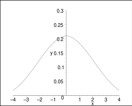
Figure 1: The shape of density $p_{ac}(x,t)$ at instant $t=2$ (for $c=1,\;\lambda=1$)

Remark 3. It is easy to check that

$$\frac{\partial}{\partial t}I_{0}\left(\frac{\lambda}{c}\sqrt{4c^{2}t^{2}-x^{2}}\right)=\frac{4\lambda ct}{\sqrt{4c^{2}t^{2}-x^{2}}}\;I_{1}\left(\frac{\lambda}{c}\sqrt{4c^{2}t^{2}-x^{2}}\right),$$ (3.16)

where $I_{1}(z)$ is the modified Bessel function of first order (see (2.6)) and, therefore, density (3.4) has the following alternative form:

$$p(x,t) =\frac{e^{-2\lambda t}}{2}\;\delta(x)+\frac{e^{-2\lambda t}}{4}\left[\delta(2ct+x)+\delta(2ct-x)\right]$$ (3.17)

$$\quad+\frac{\lambda e^{-2\lambda t}}{2c}\left[I_{0}\left(\frac{\lambda}{c}\sqrt{4c^{2}t^{2}-x^{2}}\right)+\frac{ct}{\sqrt{4c^{2}t^{2}-x^{2}}}\;I_{1}\left(\frac{\lambda}{c}\sqrt{4c^{2}t^{2}-x^{2}}\right)\right.$$

$$\qquad\qquad\qquad+\left.\frac{\lambda}{2c}\int_{|x|}^{2ct}I_{0}\left(\frac{\lambda}{c}\sqrt{\tau^{2}-x^{2}}\right)d\tau\right]\Theta(2ct-|x|),$$

$$x\in\mathbb{R},\qquad t\geq 0.$$

4 Partial Differential Equation

Consider the function

$$g(x,t)=\left(\frac{\partial}{\partial t}+2\lambda\right)p(x,t).$$ (4.1)

Here $\partial/\partial t$ means differentiation in $t$ of the generalized function $p(x,t)$. The unexpected and amazing fact is that this function satisfies the Goldstein-Kac telegraph equation with doubled parameters $2c$ and $2\lambda$. This result is given by the following theorem.

Theorem 2. Function $g(x,t)$ defined by (4.1) satisfies the telegraph equation

$$\left(\frac{\partial^{2}}{\partial t^{2}}+4\lambda\frac{\partial}{\partial t}-4c^{2}\frac{\partial^{2}}{\partial x^{2}}\right)g(x,t)=0.$$ (4.2)

Proof. Introduce a new function $w(x,t)$ by the equality

$$w(x,t)=e^{2\lambda t}g(x,t).$$

Therefore, in order to prove the theorem, we should demonstrate that function $w(x,t)$ satisfies the equation

$$\left(\frac{\partial^{2}}{\partial t^{2}}-4c^{2}\frac{\partial^{2}}{\partial x^{2}}-4\lambda^{2}\right)w(x,t)=0.$$ (4.3)

According to (4.1), we have

$$w(x,t)=e^{2\lambda t}\left(\frac{\partial}{\partial t}+2\lambda\right)p(x,t)=\frac{\partial}{\partial t}\left(e^{2\lambda t}p(x,t)\right).$$ (4.4)

To avoid differentiation of generalized function $w(x,t)$, instead we use the characteristic function approach. In view of (4.3), we need to show that the characteristic function (Fourier transform) $\hat{w}(x,t)$ satisfies the equation

$$\frac{\partial^{2}\hat{w}(\xi,t)}{\partial t^{2}}-4(\lambda^{2}-c^{2}\xi^{2})\;\hat{w}(\xi,t)=0.$$ (4.5)

According to (3.6), the characteristic function $\hat{w}(x,t)$ has the form

$$\hat{w}(\xi,t) =\frac{\partial}{\partial t}\left(e^{2\lambda t}\Psi(\xi,t)\right)$$

$$=\frac{\partial}{\partial t}\biggl{\{}\biggl{[}\cosh\left(t\sqrt{\lambda^{2}-c^{2}\xi^{2}}\right)+\frac{\lambda}{\sqrt{\lambda^{2}-c^{2}\xi^{2}}}\;\sinh\left(t\sqrt{\lambda^{2}-c^{2}\xi^{2}}\right)\biggr{]}^{2}\mathbb{1}_{\left\{|\xi|\leq\frac{\lambda}{c}\right\}}$$

$$\qquad+\biggl{[}\cos\left(t\sqrt{c^{2}\xi^{2}-\lambda^{2}}\right)+\frac{\lambda}{\sqrt{c^{2}\xi^{2}-\lambda^{2}}}\;\sin\left(t\sqrt{c^{2}\xi^{2}-\lambda^{2}}\right)\biggr{]}^{2}\mathbb{1}_{\left\{|\xi|>\frac{\lambda}{c}\right\}}\biggr{\}}$$

$$=\frac{\partial}{\partial t}\biggl{\{}\left[\cosh^{2}\left(t\sqrt{\lambda^{2}-c^{2}\xi^{2}}\right)\mathbb{1}_{\left\{|\xi|\leq\frac{\lambda}{c}\right\}}+\cos^{2}\left(t\sqrt{c^{2}\xi^{2}-\lambda^{2}}\right)\mathbb{1}_{\left\{|\xi|>\frac{\lambda}{c}\right\}}\right]$$

$$\qquad\;+\lambda\biggl{[}\frac{\sinh\left(2t\sqrt{\lambda^{2}-c^{2}\xi^{2}}\right)}{\sqrt{\lambda^{2}-c^{2}\xi^{2}}}\mathbb{1}_{\left\{|\xi|\leq\frac{\lambda}{c}\right\}}+\frac{\sin\left(2t\sqrt{c^{2}\xi^{2}-\lambda^{2}}\right)}{\sqrt{c^{2}\xi^{2}-\lambda^{2}}}\mathbb{1}_{\left\{|\xi|>\frac{\lambda}{c}\right\}}\biggr{]}$$

$$\qquad+\lambda^{2}\biggl{[}\frac{\sinh^{2}\left(t\sqrt{\lambda^{2}-c^{2}\xi^{2}}\right)}{\lambda^{2}-c^{2}\xi^{2}}\mathbb{1}_{\left\{|\xi|\leq\frac{\lambda}{c}\right\}}+\frac{\sin^{2}\left(t\sqrt{c^{2}\xi^{2}-\lambda^{2}}\right)}{c^{2}\xi^{2}-\lambda^{2}}\mathbb{1}_{\left\{|\xi|>\frac{\lambda}{c}\right\}}\biggr{]}\biggr{\}}.$$

where $\Psi(\xi,t)$ is the characteristic function of process $S(t)$ given by (3.6). Evaluating this expression, after some simple computations we arrive to the formula

$$\hat{w}(\xi,t) =\biggl{[}\sqrt{\lambda^{2}-c^{2}\xi^{2}}\sinh\left(2t\sqrt{\lambda^{2}-c^{2}\xi^{2}}\right)+2\lambda\cosh\left(2t\sqrt{\lambda^{2}-c^{2}\xi^{2}}\right)$$ (4.6)

$$\qquad\qquad\qquad\qquad\qquad+\lambda^{2}\;\frac{\sinh\left(2t\sqrt{\lambda^{2}-c^{2}\xi^{2}}\right)}{\sqrt{\lambda^{2}-c^{2}\xi^{2}}}\biggr{]}\mathbb{1}_{\left\{|\xi|\leq\frac{\lambda}{c}\right\}}$$

$$+\biggl{[}-\sqrt{c^{2}\xi^{2}-\lambda^{2}}\sin\left(2t\sqrt{c^{2}\xi^{2}-\lambda^{2}}\right)+2\lambda\cos\left(2t\sqrt{c^{2}\xi^{2}-\lambda^{2}}\right)$$

$$\qquad\qquad\qquad\qquad\qquad+\lambda^{2}\;\frac{\sin\left(2t\sqrt{c^{2}\xi^{2}-\lambda^{2}}\right)}{\sqrt{c^{2}\xi^{2}-\lambda^{2}}}\biggr{]}\mathbb{1}_{\left\{|\xi|>\frac{\lambda}{c}\right\}}.$$

Thus, we should prove that function (4.6) satisfies equation (4.5). For the first term of (4.6) we have

$$\frac{\partial^{2}}{\partial t^{2}} \biggl{[}\sqrt{\lambda^{2}-c^{2}\xi^{2}}\sinh\left(2t\sqrt{\lambda^{2}-c^{2}\xi^{2}}\right)+2\lambda\cosh\left(2t\sqrt{\lambda^{2}-c^{2}\xi^{2}}\right)$$

$$\qquad\qquad\qquad\qquad\qquad+\lambda^{2}\;\frac{\sinh\left(2t\sqrt{\lambda^{2}-c^{2}\xi^{2}}\right)}{\sqrt{\lambda^{2}-c^{2}\xi^{2}}}\biggr{]}\mathbb{1}_{\left\{|\xi|\leq\frac{\lambda}{c}\right\}}$$

$$=\biggl{[}4(\lambda^{2}-c^{2}\xi^{2})^{3/2}\sinh\left(2t\sqrt{\lambda^{2}-c^{2}\xi^{2}}\right)+8\lambda(\lambda^{2}-c^{2}\xi^{2})\cosh\left(2t\sqrt{\lambda^{2}-c^{2}\xi^{2}}\right)$$

$$\qquad\qquad\qquad\qquad\qquad+4\lambda^{2}(\lambda^{2}-c^{2}\xi^{2})^{1/2}\sinh\left(2t\sqrt{\lambda^{2}-c^{2}\xi^{2}}\right)\biggr{]}\mathbb{1}_{\left\{|\xi|\leq\frac{\lambda}{c}\right\}}$$

and therefore, for $|\xi|\leq\frac{\lambda}{c}$, we obtain

$$\frac{\partial^{2}\hat{w}(\xi,t)}{\partial t^{2}} -4(\lambda^{2}-c^{2}\xi^{2})\;\hat{w}(\xi,t)$$

$$=\biggl{[}4(\lambda^{2}-c^{2}\xi^{2})^{3/2}\sinh\left(2t\sqrt{\lambda^{2}-c^{2}\xi^{2}}\right)+8\lambda(\lambda^{2}-c^{2}\xi^{2})\cosh\left(2t\sqrt{\lambda^{2}-c^{2}\xi^{2}}\right)$$

$$\qquad\qquad\qquad\qquad\qquad+4\lambda^{2}(\lambda^{2}-c^{2}\xi^{2})^{1/2}\sinh\left(2t\sqrt{\lambda^{2}-c^{2}\xi^{2}}\right)\biggr{]}\mathbb{1}_{\left\{|\xi|\leq\frac{\lambda}{c}\right\}}$$

$$\qquad-\biggl{[}4(\lambda^{2}-c^{2}\xi^{2})\biggl{\{}\sqrt{\lambda^{2}-c^{2}\xi^{2}}\sinh\left(2t\sqrt{\lambda^{2}-c^{2}\xi^{2}}\right)+2\lambda\cosh\left(2t\sqrt{\lambda^{2}-c^{2}\xi^{2}}\right)$$

$$\qquad\qquad\qquad\qquad\qquad+\lambda^{2}\;\frac{\sinh\left(2t\sqrt{\lambda^{2}-c^{2}\xi^{2}}\right)}{\sqrt{\lambda^{2}-c^{2}\xi^{2}}}\biggr{\}}\biggr{]}\mathbb{1}_{\left\{|\xi|\leq\frac{\lambda}{c}\right\}}$$

$$=0$$

proving (4.5). The proof for the second term of (4.6) for $|\xi|>\frac{\lambda}{c}$ is similar. The theorem is proved. $\square$

Remark 4. From (4.1) and (4.2) it follows that the transition probability density $p(x,t)$ of process $S(t)$ satisfies the third-order hyperbolic partial differential equation

$$\left(\frac{\partial}{\partial t}+2\lambda\right)\left(\frac{\partial^{2}}{\partial t^{2}}+4\lambda\frac{\partial}{\partial t}-4c^{2}\frac{\partial^{2}}{\partial x^{2}}\right)p(x,t)=0.$$ (4.7)

Note that differential operator in (4.7) represents the product of the standard Goldstein-Kac telegraph operator with doubled parameters $2c,\;2\lambda$ and shifted time differential operator. This interesting fact means that, while the densities of two independent telegraph processes $X_{1}(t)$ and $X_{2}(t)$ satisfy the second-order telegraph equation (2.3), their convolution (that is, the density $p(x,t)$ of the sum $S(t)=X_{1}(t)+X_{2}(t)$) satisfies third-order equation (4.7). By differentiating in $t$ the characteristic function $\Psi(\xi,t)$ given by (3.6) one can easily show that

$$\Psi(\xi,t)\bigr{|}_{t=0}=1,\qquad\frac{\partial\Psi(\xi,t)}{\partial t}\biggr{|}_{t=0}=0,\qquad\frac{\partial^{2}\Psi(\xi,t)}{\partial t^{2}}\biggr{|}_{t=0}=-2c^{2}\xi^{2},$$

and, therefore, in contrast to (2.5), the density $p(x,t)$ of process $S(t)$ is not the fundamental solution to equation (4.7).

5 Probability Distribution Function

In this section we concentrate our efforts on deriving a closed-form expression for the probability distribution function

$$\Phi(x,t)=\text{Pr}\left\{S(t)<x\right\},\qquad x\in\mathbb{R},\quad t>0,$$

of the process $S(t)$. This result is given by the following theorem.

Theorem 3. The probability distribution function $\Phi(x,t)$ has the form:

$$\Phi(x,t)=\left\{\begin{aligned} 0,\qquad\qquad&\text{if}\;\;x\in(-\infty,\;-2ct],\\ G^{-}(x,t),\qquad&\text{if}\;\;x\in(-2ct,\;0],\\ G^{+}(x,t),\qquad&\text{if}\;\;x\in(0,\;2ct],\\ 1,\qquad\qquad&\text{if}\;\;x\in(2ct,\;+\infty),\end{aligned}\right.\qquad t>0,$$ (5.1)

where functions $G^{\pm}(x,t)$ are given by the formula:

$$G^{\pm}(x,t) =\frac{1}{2}\pm\frac{e^{-2\lambda t}}{4}\cos\left(\frac{\lambda x}{c}\right)+\frac{\lambda xe^{-2\lambda t}}{2c}\biggl{[}\sum_{k=0}^{\infty}\frac{(\lambda t)^{2k}}{(k!)^{2}}\left(1+\frac{\lambda t}{2k+2}\right)F\left(-k,\frac{1}{2};\frac{3}{2};\frac{x^{2}}{4c^{2}t^{2}}\right)$$ (5.2)

$$\hskip 85.35826pt+\sum_{k=0}^{\infty}\frac{(\lambda t)^{2k+1}}{(k!)^{2}\;(2k+1)}\;_{3}F_{2}\left(-k,-k-\frac{1}{2},\frac{1}{2};\;-k+\frac{1}{2},\frac{3}{2};\;\frac{x^{2}}{4c^{2}t^{2}}\right)\biggr{]}.$$

Here $F(\alpha,\beta;\gamma;z)$ is the Gauss hypergeometric function given by (2.11) and

$$_{3}F_{2}(\alpha,\beta,\gamma;\xi,\zeta;z)=\sum_{k=0}^{\infty}\frac{(\alpha)_{k}\;(\beta)_{k}\;(\gamma)_{k}}{(\xi)_{k}\;(\zeta)_{k}}\;\frac{z^{k}}{k!}$$ (5.3)

is the generalized hypergeometric functions.

Proof. Formula (5.1) in the intervals $x\in(-\infty,\;-2ct]$ and $x\in(2ct,\;+\infty)$ is obvious. Therefore, it remains to prove (5.1) for $x\in(-2ct,\;2ct]$.

Since $x=0$ is a singularity point, then for arbitrary $x\in(-2ct,\;2ct]$ we have

$$\Phi(x,t)=\text{Pr}\left\{S(t)=-2ct\right\}+\text{Pr}\left\{S(t)=0\right\}\Theta(x)+\text{Pr}\left\{S(t)\in R_{x}\right\},$$

where

$$R_{x}=\left\{\begin{aligned} (-2ct,\;x),\qquad&\text{if}\;x\in(-2ct,\;0],\\ (-2ct,\;x)-\{0\},\qquad&\text{if}\;x\in(0,\;2ct]\end{aligned}\right.$$

and $\Theta(x)$ is the Heaviside step function given by (2.7).

Taking into account (3.1) and (3.2), we get

$$\Phi(x,t)=\frac{e^{-2\lambda t}}{4}+\frac{e^{-2\lambda t}}{2}\Theta(x)+\text{Pr}\left\{S(t)\in R_{x}\right\}.$$ (5.4)

Thus, our aim is to evaluate the term $\text{Pr}\left\{S(t)\in R_{x}\right\}$ for $x\in(-2ct,\;2ct]$.

Integrating the absolutely continuous part of density (3.17), we have for arbitrary $x\in(-2ct,\;2ct]$:

$$\text{Pr}\{S(t)\in R_{x}\} =\frac{\lambda e^{-2\lambda t}}{2c}\biggl{[}\int_{-2ct}^{x}I_{0}\left(\frac{\lambda}{c}\sqrt{4c^{2}t^{2}-z^{2}}\right)dz+ct\int_{-2ct}^{x}\frac{I_{1}\left(\frac{\lambda}{c}\sqrt{4c^{2}t^{2}-z^{2}}\right)}{\sqrt{4c^{2}t^{2}-z^{2}}}dz$$ (5.5)

$$\qquad\qquad\qquad+\frac{\lambda}{2c}\int_{-2ct}^{x}\biggl{\{}\int_{|z|}^{2ct}I_{0}\left(\frac{\lambda}{c}\sqrt{\tau^{2}-z^{2}}\biggr{)}d\tau\right\}\;dz\biggr{]}.$$

To evaluate the integrals on the right-hand side of (5.5), we need the following relations (see [17, formulas (6.3) and (6.4) therein]):

$$\int I_{0}(b\sqrt{a^{2}-z^{2}})\;dz=z\sum_{k=0}^{\infty}\frac{1}{(k!)^{2}}\left(\frac{ab}{2}\right)^{2k}F\left(-k,\frac{1}{2};\frac{3}{2};\frac{z^{2}}{a^{2}}\right)+\psi_{1},$$ (5.6)

$$\int\frac{I_{1}(b\sqrt{a^{2}-z^{2}})}{\sqrt{a^{2}-z^{2}}}\;dz=\frac{z}{a}\sum_{k=0}^{\infty}\frac{1}{k!\;(k+1)!}\left(\frac{ab}{2}\right)^{2k+1}F\left(-k,\frac{1}{2};\frac{3}{2};\frac{z^{2}}{a^{2}}\right)+\psi_{2},$$ (5.7)

$$|z|\leq a,\quad a>0,\quad b\geq 0,$$

where $F(\alpha,\beta;\gamma;z)$ is the Gauss hypergeometric function with series representation given by the first formula of (5.3) and $\psi_{1},\;\psi_{2}$ are arbitrary functions not depending on $z$. Applying formula (5.6) to the first integral in (5.5), we get

$$\int\limits_{-2ct}^{x}I_{0}\left(\frac{\lambda}{c}\sqrt{4c^{2}t^{2}-z^{2}}\right)dz=x\sum_{k=0}^{\infty}\frac{(\lambda t)^{2k}}{(k!)^{2}}F\left(-k,\frac{1}{2};\frac{3}{2};\frac{x^{2}}{4c^{2}t^{2}}\right)+2ct\sum_{k=0}^{\infty}\frac{(\lambda t)^{2k}}{(k!)^{2}}F\left(-k,\frac{1}{2};\frac{3}{2};1\right).$$

In view of the formula

$$F\left(-k,\frac{1}{2};\frac{3}{2};1\right)=\frac{(2k)!!}{(2k+1)!!}=\frac{2^{k}\;k!}{(2k+1)!!},\qquad k\geq 0,$$ (5.8)

the second term is found to be

$$2ct\sum_{k=0}^{\infty}\frac{(\lambda t)^{2k}}{(k!)^{2}}F\left(-k,\frac{1}{2};\frac{3}{2};1\right)=\frac{c}{\lambda}\sinh(2\lambda t)$$

and we obtain for arbitrary $x\in(-2ct,2ct]$:

$$\int\limits_{-2ct}^{x}I_{0}\left(\frac{\lambda}{c}\sqrt{4c^{2}t^{2}-z^{2}}\right)dz=x\sum_{k=0}^{\infty}\frac{(\lambda t)^{2k}}{(k!)^{2}}F\left(-k,\frac{1}{2};\frac{3}{2};\frac{x^{2}}{4c^{2}t^{2}}\right)+\frac{c}{\lambda}\sinh(2\lambda t).$$ (5.9)

According to (5.7), the second integral in (5.5) is

$$\int_{-2ct}^{x}\frac{I_{1}\left(\frac{\lambda}{c}\sqrt{4c^{2}t^{2}-z^{2}}\right)}{\sqrt{4c^{2}t^{2}-z^{2}}}dz =\frac{x}{2ct}\sum_{k=0}^{\infty}\frac{(\lambda t)^{2k+1}}{k!\;(k+1)!}F\left(-k,\frac{1}{2};\frac{3}{2};\frac{x^{2}}{4c^{2}t^{2}}\right)$$

$$\qquad\qquad+\sum_{k=0}^{\infty}\frac{(\lambda t)^{2k+1}}{k!\;(k+1)!}F\left(-k,\frac{1}{2};\frac{3}{2};1\right).$$

Applying (5.8) one can easily show that the second term is

$$\sum_{k=0}^{\infty}\frac{(\lambda t)^{2k+1}}{k!\;(k+1)!}F\left(-k,\frac{1}{2};\frac{3}{2};1\right)=\frac{1}{2\lambda t}\left(\cosh(2\lambda t)-1\right)$$

and, therefore, we obtain for arbitrary $x\in(-2ct,2ct]$:

$$\int_{-2ct}^{x}\frac{I_{1}\left(\frac{\lambda}{c}\sqrt{4c^{2}t^{2}-z^{2}}\right)}{\sqrt{4c^{2}t^{2}-z^{2}}}dz=\frac{x}{2ct}\sum_{k=0}^{\infty}\frac{(\lambda t)^{2k+1}}{k!\;(k+1)!}F\left(-k,\frac{1}{2};\frac{3}{2};\frac{x^{2}}{4c^{2}t^{2}}\right)+\frac{1}{2\lambda t}\left(\cosh(2\lambda t)-1\right).$$ (5.10)

For the third (double) integral in (5.5) we have for arbitrary $x\in(-2ct,\;2ct]$:

$$\int_{-2ct}^{x} \biggl{\{}\int_{|z|}^{2ct}I_{0}\left(\frac{\lambda}{c}\sqrt{\tau^{2}-z^{2}}\biggr{)}d\tau\right\}dz$$ (5.11)

$$=\int_{-2ct}^{x}\biggl{\{}\int_{0}^{2ct}I_{0}\left(\frac{\lambda}{c}\sqrt{\tau^{2}-z^{2}}\right)\mathbb{1}_{\{\tau>|z|\}}\;d\tau\biggr{\}}dz$$

$$=\int_{0}^{2ct}\biggl{\{}\int_{-2ct}^{x}I_{0}\left(\frac{\lambda}{c}\sqrt{\tau^{2}-z^{2}}\right)\mathbb{1}_{\{|z|<\tau\}}\;dz\biggr{\}}d\tau$$

$$=\int_{0}^{2ct}\biggl{\{}\int_{-\tau}^{\min\{x,\tau\}}I_{0}\left(\frac{\lambda}{c}\sqrt{\tau^{2}-z^{2}}\right)dz\biggr{\}}\mathbb{1}_{\{-\tau<\min\{x,\tau\}\}}\;d\tau.$$

Now we should separately consider two possible cases when $x$ is negative and positive.

$\bullet$ The case $x\in(-2ct,\;0]$. In this case $x$ is non-positive and, therefore, (5.11) takes the form:

$$\int_{-2ct}^{x}\biggl{\{}\int_{|z|}^{2ct}I_{0}\left(\frac{\lambda}{c}\sqrt{\tau^{2}-z^{2}}\biggr{)}d\tau\right\}dz =\int_{0}^{2ct}\biggl{\{}\int_{-\tau}^{x}I_{0}\left(\frac{\lambda}{c}\sqrt{\tau^{2}-z^{2}}\right)dz\biggr{\}}\mathbb{1}_{\{-\tau<x\}}\;d\tau$$ (5.12)

$$=\int_{-x}^{2ct}\biggl{\{}\int_{-\tau}^{x}I_{0}\left(\frac{\lambda}{c}\sqrt{\tau^{2}-z^{2}}\right)dz\biggr{\}}d\tau.$$

According to (5.6), the interior integral in curl brackets is:

$$\int_{-\tau}^{x}I_{0}\left(\frac{\lambda}{c}\sqrt{\tau^{2}-z^{2}}\right)dz =x\sum_{k=0}^{\infty}\frac{1}{(k!)^{2}}\left(\frac{\lambda}{2c}\tau\right)^{2k}F\left(-k,\frac{1}{2};\frac{3}{2};\frac{x^{2}}{\tau^{2}}\right)$$

$$\hskip 14.22636pt+\tau\sum_{k=0}^{\infty}\frac{1}{(k!)^{2}}\left(\frac{\lambda}{2c}\tau\right)^{2k}F\left(-k,\frac{1}{2};\frac{3}{2};1\right).$$

Applying again (5.8) we easily evaluate the second term

$$\tau\sum_{k=0}^{\infty}\frac{1}{(k!)^{2}}\left(\frac{\lambda}{2c}\tau\right)^{2k}F\left(-k,\frac{1}{2};\frac{3}{2};1\right)=\frac{c}{\lambda}\sinh\left(\frac{\lambda}{c}\tau\right)$$

and, therefore, we get

$$\int_{-\tau}^{x}I_{0}\left(\frac{\lambda}{c}\sqrt{\tau^{2}-z^{2}}\right)dz=x\sum_{k=0}^{\infty}\frac{1}{(k!)^{2}}\left(\frac{\lambda}{2c}\tau\right)^{2k}F\left(-k,\frac{1}{2};\frac{3}{2};\frac{x^{2}}{\tau^{2}}\right)+\frac{c}{\lambda}\sinh\left(\frac{\lambda}{c}\tau\right).$$ (5.13)

Substituting this into (5.12) we obtain:

$$\int_{-2ct}^{x}\biggl{\{}\int_{|z|}^{2ct}I_{0}\left(\frac{\lambda}{c}\sqrt{\tau^{2}-z^{2}}\biggr{)}d\tau\right\}\;dz$$ (5.14)

$$=x\sum_{k=0}^{\infty}\frac{1}{(k!)^{2}}\left(\frac{\lambda}{2c}\right)^{2k}\int_{-x}^{2ct}\tau^{2k}F\left(-k,\frac{1}{2};\frac{3}{2};\frac{x^{2}}{\tau^{2}}\right)d\tau+\frac{c}{\lambda}\int_{-x}^{2ct}\sinh\left(\frac{\lambda}{c}\tau\right)d\tau.$$

Here we have used the easily checked fact that, for arbitrary $x\in(-2ct,\;2ct]$, the following uniform (in $\tau\in(0,\;2ct)$) estimate

$$\left|\tau^{2k}F\left(-k,\frac{1}{2};\frac{3}{2};\frac{x^{2}}{\tau^{2}}\right)\right|<(4ct)^{2k}$$

holds and, therefore, the series in (5.13) converges uniformly in $\tau\in(0,\;2ct)$.

The second term on the right-hand side of (5.14) is found to be

$$\frac{c}{\lambda}\int_{-x}^{2ct}\sinh\left(\frac{\lambda}{c}\tau\right)d\tau=\frac{c^{2}}{\lambda^{2}}\left[\cosh(2\lambda t)-\cosh\left(\frac{\lambda}{c}x\right)\right].$$ (5.15)

Applying formula (7.10) of Lemma A4 (see below), we have for the integral of the first term on the right-hand side of (5.14):

$$\int_{-x}^{2ct}\tau^{2k}F\left(-k,\frac{1}{2};\frac{3}{2};\frac{x^{2}}{\tau^{2}}\right)d\tau =\frac{(2ct)^{2k+1}}{2k+1}\;_{3}F_{2}\left(-k,-k-\frac{1}{2},\frac{1}{2};\;-k+\frac{1}{2},\frac{3}{2};\;\frac{x^{2}}{4c^{2}t^{2}}\right)$$ (5.16)

$$\qquad+\frac{x^{2k+1}}{2k+1}\;_{3}F_{2}\left(-k,-k-\frac{1}{2},\frac{1}{2};\;-k+\frac{1}{2},\frac{3}{2};\;1\right).$$

Using the well-known formulas for Pochhammer symbol

$$(-k)_{s} =(-1)^{s}\;\frac{k!}{(k-s)!},\qquad 0\leq s\leq k,\quad k\geq 0,$$ (5.17)

$$\frac{(a)_{s}}{(a+1)_{s}} =\frac{a}{a+s},\qquad s\geq 0,\quad\quad a\in\mathbb{R},$$

and some simple combinatorial relations, one can check that

$${}_{3}F_{2}\left(-k,-k-\frac{1}{2},\frac{1}{2};\;-k+\frac{1}{2},\frac{3}{2};\;1\right) =(2k+1)\sum_{s=0}^{k}\frac{(-1)^{s}}{(2s+1)(2k-2s+1)}\;\binom{k}{s}$$

$$=\left\{\begin{aligned} \frac{2^{k}\;k!}{(k+1)\;(2k-1)!!},\qquad&\text{if $k$ is even},\\ 0,\qquad\qquad&\text{if $k$ is odd}.\end{aligned}\right.$$

Therefore, (5.16) takes the form:

$$\int_{-x}^{2ct}\tau^{2k}F\left(-k,\frac{1}{2};\frac{3}{2};\frac{x^{2}}{\tau^{2}}\right)d\tau =\frac{(2ct)^{2k+1}}{2k+1}\;_{3}F_{2}\left(-k,-k-\frac{1}{2},\frac{1}{2};\;-k+\frac{1}{2},\frac{3}{2};\;\frac{x^{2}}{4c^{2}t^{2}}\right)$$ (5.18)

$$\qquad+\left\{\begin{aligned} \frac{2^{k}\;k!\;\;x^{2k+1}}{(k+1)\;(2k+1)!!},\qquad&\text{if $k$ is even},\\ 0,\qquad\qquad&\text{if $k$ is odd}.\end{aligned}\right.$$

Substituting now (5.18) and (5.15) into (5.14) and taking into account that

$$x\sum_{\begin{subarray}{c}k=0\\ k\;\text{is even}\end{subarray}}^{\infty}\frac{1}{(k!)^{2}}\left(\frac{\lambda}{2c}\right)^{2k}\frac{2^{k}\;k!\;\;x^{2k+1}}{(k+1)\;(2k+1)!!}=\frac{c^{2}}{\lambda^{2}}\left[\cosh\left(\frac{\lambda}{c}x\right)-\cos\left(\frac{\lambda}{c}x\right)\right],$$ (5.19)

we obtain, for arbitrary $x\in(-2ct,\;0]$, the following formula:

$$\int_{-2ct}^{x} \biggl{\{}\int_{|z|}^{2ct}I_{0}\left(\frac{\lambda}{c}\sqrt{\tau^{2}-z^{2}}\biggr{)}d\tau\right\}dz$$ (5.20)

$$=\frac{2cx}{\lambda}\sum_{k=0}^{\infty}\frac{(\lambda t)^{2k+1}}{(k!)^{2}\;(2k+1)}\;_{3}F_{2}\left(-k,-k-\frac{1}{2},\frac{1}{2};\;-k+\frac{1}{2},\frac{3}{2};\;\frac{x^{2}}{4c^{2}t^{2}}\right)$$

$$\qquad+\frac{c^{2}}{\lambda^{2}}\left[\cosh(2\lambda t)-\cos\left(\frac{\lambda}{c}x\right)\right],\qquad\text{for}\;x\in(-2ct,\;0].$$

Substituting (5.9), (5.10) and (5.20) into (5.5), after some simple computations, we get for arbitrary $x\in(-2ct,\;0]$:

$$\text{Pr}\{S(t)\in R_{x}\} =\frac{1}{2}-\frac{e^{-2\lambda t}}{2}\cos^{2}\left(\frac{\lambda}{2c}x\right)$$ (5.21)

$$+\frac{\lambda xe^{-2\lambda t}}{2c}\biggl{[}\sum_{k=0}^{\infty}\frac{(\lambda t)^{2k}}{(k!)^{2}}\left(1+\frac{\lambda t}{2k+2}\right)F\left(-k,\frac{1}{2};\;\frac{3}{2};\;\frac{x^{2}}{4c^{2}t^{2}}\right)$$

$$\hskip 42.67912pt+\sum_{k=0}^{\infty}\frac{(\lambda t)^{2k+1}}{(k!)^{2}\;(2k+1)}\;_{3}F_{2}\left(-k,-k-\frac{1}{2},\frac{1}{2};\;-k+\frac{1}{2},\frac{3}{2};\;\frac{x^{2}}{4c^{2}t^{2}}\right)\biggr{]}.$$

Substituting (5.21) into (5.4), we finally obtain function $G^{-}(x,t)$ defined in the interval $x\in(-2ct,\;0]$ and given by formula (5.2).

$\bullet$ The case $x\in(0,\;2ct]$. In this case $x$ is strictly positive and, therefore, (5.11) yields:

$$\int_{-2ct}^{x} \biggl{\{}\int_{|z|}^{2ct}I_{0}\left(\frac{\lambda}{c}\sqrt{\tau^{2}-z^{2}}\biggr{)}d\tau\right\}dz$$ (5.22)

$$=\int_{0}^{2ct}\biggl{\{}\int_{-\tau}^{\min\{x,\tau\}}I_{0}\left(\frac{\lambda}{c}\sqrt{\tau^{2}-z^{2}}\right)dz\biggr{\}}\;d\tau$$

$$=\int_{0}^{2ct}\biggl{\{}\int_{-\tau}^{x}I_{0}\left(\frac{\lambda}{c}\sqrt{\tau^{2}-z^{2}}\right)dz\biggr{\}}\mathbb{1}_{\{\tau\geq x\}}\;d\tau$$

$$\hskip 56.9055pt+\int_{0}^{2ct}\biggl{\{}\int_{-\tau}^{\tau}I_{0}\left(\frac{\lambda}{c}\sqrt{\tau^{2}-z^{2}}\right)dz\biggr{\}}\mathbb{1}_{\{\tau<x\}}\;d\tau$$

$$=\int_{x}^{2ct}\biggl{\{}\int_{-\tau}^{x}I_{0}\left(\frac{\lambda}{c}\sqrt{\tau^{2}-z^{2}}\right)dz\biggr{\}}\;d\tau$$

$$\hskip 56.9055pt+\int_{0}^{x}\biggl{\{}\int_{-\tau}^{\tau}I_{0}\left(\frac{\lambda}{c}\sqrt{\tau^{2}-z^{2}}\right)dz\biggr{\}}\;d\tau.$$

Applying (5.13), we get for the first integral on the right-hand side of (5.22):

$$\int_{x}^{2ct} \biggl{\{}\int_{-\tau}^{x}I_{0}\left(\frac{\lambda}{c}\sqrt{\tau^{2}-z^{2}}\right)dz\biggr{\}}\;d\tau$$

$$=x\sum_{k=0}^{\infty}\frac{1}{(k!)^{2}}\left(\frac{\lambda}{2c}\right)^{2k}\int_{x}^{2ct}\tau^{2k}F\left(-k,\frac{1}{2};\frac{3}{2};\frac{x^{2}}{\tau^{2}}\right)d\tau+\frac{c}{\lambda}\int_{x}^{2ct}\sinh\left(\frac{\lambda}{c}\tau\right)d\tau.$$

Replacing $-x\mapsto x$ in (5.15) and (5.18), we get these integrals:

$$\frac{c}{\lambda}\int_{x}^{2ct}\sinh\left(\frac{\lambda}{c}\tau\right)d\tau=\frac{c^{2}}{\lambda^{2}}\left[\cosh(2\lambda t)-\cosh\left(\frac{\lambda}{c}x\right)\right]$$

$$\int_{x}^{2ct}\tau^{2k}F\left(-k,\frac{1}{2};\frac{3}{2};\frac{x^{2}}{\tau^{2}}\right)d\tau =\frac{(2ct)^{2k+1}}{2k+1}\;_{3}F_{2}\left(-k,-k-\frac{1}{2},\frac{1}{2};\;-k+\frac{1}{2},\frac{3}{2};\;\frac{x^{2}}{4c^{2}t^{2}}\right)$$

$$\qquad-\left\{\begin{aligned} \frac{2^{k}\;k!\;\;x^{2k+1}}{(k+1)\;(2k+1)!!},\qquad&\text{if $k$ is even},\\ 0,\qquad\qquad&\text{if $k$ is odd},\end{aligned}\right.$$

and, therefore, taking into account (5.19), after some simple calculations we arrive to the following formula valid for arbitrary $x\in(0,\;2ct]$:

$$\int_{x}^{2ct} \biggl{\{}\int_{-\tau}^{x}I_{0}\left(\frac{\lambda}{c}\sqrt{\tau^{2}-z^{2}}\right)dz\biggr{\}}\;d\tau$$ (5.23)

$$=\frac{2cx}{\lambda}\sum_{k=0}^{\infty}\frac{(\lambda t)^{2k+1}}{(k!)^{2}\;(2k+1)}\;_{3}F_{2}\left(-k,-k-\frac{1}{2},\frac{1}{2};\;-k+\frac{1}{2},\frac{3}{2};\;\frac{x^{2}}{4c^{2}t^{2}}\right)$$

$$\qquad+\frac{c^{2}}{\lambda^{2}}\left[\cosh(2\lambda t)-2\cosh\left(\frac{\lambda}{c}x\right)+\cos\left(\frac{\lambda}{c}x\right)\right],\qquad\text{for}\;x\in(0,\;2ct].$$

Taking into account that

$$\int_{-\tau}^{\tau}I_{0}\left(\frac{\lambda}{c}\sqrt{\tau^{2}-z^{2}}\right)dz=\frac{2c}{\lambda}\sinh\left(\frac{\lambda}{c}\tau\right),$$

we can easily evaluate the second integral on the right-hand side of (5.22):

$$\int_{0}^{x}\biggl{\{}\int_{-\tau}^{\tau}I_{0}\left(\frac{\lambda}{c}\sqrt{\tau^{2}-z^{2}}\right)dz\biggr{\}}\;d\tau=\frac{2c^{2}}{\lambda^{2}}\left[\cosh\left(\frac{\lambda}{c}x\right)-1\right],\qquad\text{for}\;x\in(0,\;2ct].$$ (5.24)

Substituting (5.23) and (5.24) into (5.22), we obtain:

$$\int_{-2ct}^{x} \biggl{\{}\int_{|z|}^{2ct}I_{0}\left(\frac{\lambda}{c}\sqrt{\tau^{2}-z^{2}}\biggr{)}d\tau\right\}dz$$ (5.25)

$$=\frac{2cx}{\lambda}\sum_{k=0}^{\infty}\frac{(\lambda t)^{2k+1}}{(k!)^{2}\;(2k+1)}\;_{3}F_{2}\left(-k,-k-\frac{1}{2},\frac{1}{2};\;-k+\frac{1}{2},\frac{3}{2};\;\frac{x^{2}}{4c^{2}t^{2}}\right)$$

$$\qquad+\frac{c^{2}}{\lambda^{2}}\left[\cosh(2\lambda t)+\cos\left(\frac{\lambda}{c}x\right)-2\right],\qquad\text{for}\;x\in(0,\;2ct].$$

Substituting now (5.9), (5.10) and (5.25) into (5.5), after some simple computations, we obtain the following formula valid for arbitrary $x\in(0,\;2ct]$:

$$\text{Pr}\{S(t)\in R_{x}\} =\frac{1}{2}-\frac{e^{-2\lambda t}}{4}\left(3-\cos\left(\frac{\lambda}{c}x\right)\right)$$ (5.26)

$$+\frac{\lambda xe^{-2\lambda t}}{2c}\biggl{[}\sum_{k=0}^{\infty}\frac{(\lambda t)^{2k}}{(k!)^{2}}\left(1+\frac{\lambda t}{2k+2}\right)F\left(-k,\frac{1}{2};\;\frac{3}{2};\;\frac{x^{2}}{4c^{2}t^{2}}\right)$$

$$\hskip 28.45274pt+\sum_{k=0}^{\infty}\frac{(\lambda t)^{2k+1}}{(k!)^{2}\;(2k+1)}\;_{3}F_{2}\left(-k,-k-\frac{1}{2},\frac{1}{2};\;-k+\frac{1}{2},\frac{3}{2};\;\frac{x^{2}}{4c^{2}t^{2}}\right)\biggr{]},$$

$$\text{for}\;x\in(0,\;2ct].$$

Substituting (5.26) into (5.4) we obtain function $G^{+}(x,t)$ defined in the interval $x\in(0,\;2ct]$ and given by formula (5.2). The theorem is thus completely proved. $\square$

The shape of probability distribution function $\Phi(x,t)$ at time instant $t=1.5$ given by formulas (5.1)-(5.2) for the particular values of parameters $c=2,\;\lambda=0.8$ in the interval $x\in(-6,\;6]$ is presented in Fig. 2.

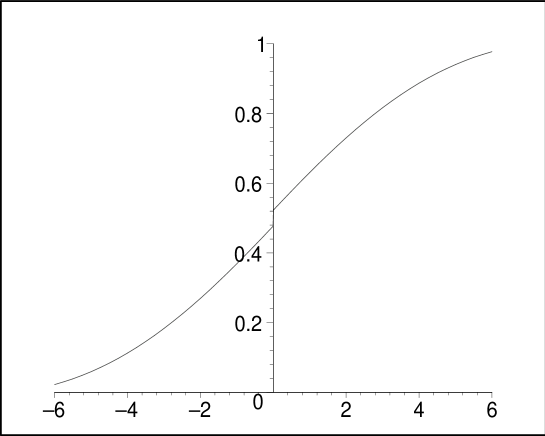
Figure 2: The shape of p.d.f. $\Phi(x,t)$ at time instant $t=1.5$ (for $c=2,\;\lambda=0.8$)

We see that distribution function $\Phi(x,t)$ is left-continuous with jumps at the origin $x=0$ and at the terminal points $x=\pm 2ct$ determined by the singularities concentrated at these three points. Obviously,

$$\lim\limits_{x\to 0-0}G^{-}(x,t)=G^{-}(0,t)=\frac{1}{2}-\frac{e^{-2\lambda t}}{4},\qquad\lim\limits_{x\to 0+0}G^{+}(x,t)=\frac{1}{2}+\frac{e^{-2\lambda t}}{4}$$

and, therefore, at the origin $x=0$ function $\Phi(x,t)$ has jump of the amplitude

$$\lim\limits_{x\to 0+0}G^{+}(x,t)-\lim\limits_{x\to 0-0}G^{-}(x,t)=\frac{e^{-2\lambda t}}{2}.$$

This entirely accords with (3.2). One can also check that

$$\lim\limits_{x\to-2ct+0}G^{-}(x,t)=\frac{e^{-2\lambda t}}{4},\qquad\lim\limits_{x\to 2ct-0}G^{+}(x,t)=G^{+}(2ct,t)=1-\frac{e^{-2\lambda t}}{4}$$ (5.27)

and, hence, function $\Phi(x,t)$ has jumps of the same amplitude $e^{-2\lambda t}/4$ at the terminal points $x=\pm 2ct$. This also entirely accords with (3.1).

Remark 5. Notice that the first series in functions $G^{\pm}(x,t)$ containing Gauss hypergeometric function plus 1/2 is quite similar to the probability distribution function (2.10) of the Goldstein-Kac telegraph process.

Remark 6. Probability distribution function $\Phi(x,t)$ has very interesting and unexpected peculiarity. Both the functions $G^{\pm}(x,t)$ contain an oscillating term determined by the presence of the cosine function $\pm\cos\left(\frac{\lambda}{c}x\right)$. On the other hand, we see that $G^{\pm}(x,t)$ are strictly positive and monotonously increasing functions as they must be. The explanation of this unusual fact is that the second series in $G^{\pm}(x,t)$ that includes the hypergeometric function ${}_{3}F_{2}\left(-k,-k-\frac{1}{2},\frac{1}{2};\;-k+\frac{1}{2},\frac{3}{2};\;\frac{x^{2}}{4c^{2}t^{2}}\right)$ converges uniformly in $x\in[-2ct,\;2ct]$ and contains an infinite number of terms that form a hidden oscillating term with the cosine function $\mp\cos\left(\frac{\lambda}{c}x\right)$ of the opposite sign and, therefore, these oscillating terms annihilate each other. This interesting phenomenon can be observed when computing the limits (5.27). The appearance of such oscillating terms in functions $G^{\pm}(x,t)$ (which are, in fact, the convolution of two probability distribution functions of the telegraph processes $X_{1}(t)$ and $X_{2}(t)$) is a fairly unusual fact that can, apparently, be explained by some properties of the convolution operation.

Remark 7. Using the relation (see [23, item 7.4.1, formula 5]):

$${}_{3}F_{2} \left(-k,-k-\frac{1}{2},\frac{1}{2};\;-k+\frac{1}{2},\frac{3}{2};\;\frac{x^{2}}{4c^{2}t^{2}}\right)$$

$$=\frac{1}{2k+2}F\left(-k-\frac{1}{2},-k;\;-k+\frac{1}{2};\;\frac{x^{2}}{4c^{2}t^{2}}\right)+\frac{2k+1}{2k+2}F\left(-k,\frac{1}{2};\;\frac{3}{2};\;\frac{x^{2}}{4c^{2}t^{2}}\right),$$

we can represent probability distribution function $\Phi(x,t)$ in terms of solely Gauss hypergeometric function with the following alternative form of functions $G^{\pm}(x,t)$:

$$G^{\pm}(x,t) =\frac{1}{2}\pm\frac{e^{-2\lambda t}}{4}\cos\left(\frac{\lambda x}{c}\right)+\frac{\lambda xe^{-2\lambda t}}{2c}\biggl{[}\sum_{k=0}^{\infty}\frac{(\lambda t)^{2k}}{(k!)^{2}}\left(1+\frac{\lambda t}{k+1}\right)F\left(-k,\frac{1}{2};\frac{3}{2};\frac{x^{2}}{4c^{2}t^{2}}\right)$$ (5.28)

$$\hskip 85.35826pt+\sum_{k=0}^{\infty}\frac{(\lambda t)^{2k+1}}{(k!)^{2}\;(2k+1)(2k+2)}\;F\left(-k,-k-\frac{1}{2};\;-k+\frac{1}{2};\;\frac{x^{2}}{4c^{2}t^{2}}\right)\biggr{]}.$$

6 Some Remarks on the General Case

The results obtained above concern the case when both telegraph processes start from the origin $0\in\mathbb{R}$ and have the same parameters $c$ and $\lambda$. The most general case implies that the processes may have different parameters and may start from two different points of $\mathbb{R}$. While the method developed in this article works also in this situation, the analysis seems to be much more complicated and explicit formulas for the distribution of the sum of the processes can scarcely be obtained. In this section we give some hints concerning such general case.

Denote by $X^{x^{0}}(t)$ the telegraph process starting from some arbitrary point $x^{0}\in\mathbb{R}$. It is clear that the transition density of $X^{x^{0}}(t)$ emerges from (2.5) by the formal replacement $x\mapsto x-x^{0}$ and it has the form

$$f_{x^{0}}(x,t) =\frac{e^{-\lambda t}}{2}\left[\delta(ct-(x-x^{0}))+\delta(ct+(x-x^{0}))\right]$$ (6.1)

$$+\frac{\lambda e^{-\lambda t}}{2c}\left[I_{0}\left(\frac{\lambda}{c}\sqrt{c^{2}t^{2}-(x-x^{0})^{2}}\right)+ct\frac{I_{0}\left(\frac{\lambda}{c}\sqrt{c^{2}t^{2}-(x-x^{0})^{2}}\right)}{\sqrt{c^{2}t^{2}-(x-x^{0})^{2}}}\right]\Theta(ct-|x-x^{0}|).$$

The support of the distribution of $X^{x^{0}}(t)$ is the close interval $[x^{0}-ct,x^{0}+ct]$. The first term in (6.1)

$$f_{s}^{x^{0}}(x,t)=\frac{e^{-\lambda t}}{2}\left[\delta(ct-(x-x^{0}))+\delta(ct+(x-x^{0}))\right]$$ (6.2)

is the singular part of the density concentrated at two terminal points $x^{0}\pm ct$ of the interval, while the second term

$$f_{ac}^{x^{0}}(x,t)=\frac{\lambda e^{-\lambda t}}{2c}\left[I_{0}\left(\frac{\lambda}{c}\sqrt{c^{2}t^{2}-(x-x^{0})^{2}}\right)+ct\frac{I_{0}\left(\frac{\lambda}{c}\sqrt{c^{2}t^{2}-(x-x^{0})^{2}}\right)}{\sqrt{c^{2}t^{2}-(x-x^{0})^{2}}}\right]\Theta(ct-|x-x^{0}|).$$ (6.3)

is the density of the absolutely continuous part of the distribution of $X^{x^{0}}(t)$ concentrated in the open interval $(x^{0}-ct,x^{0}+ct)$.

The characteristic function of process $X^{x^{0}}(t)$ has the form

$$H^{x^{0}}(\xi,t)=e^{i\xi x^{0}}H(\xi,t),\qquad\xi\in\mathbb{R},\quad t\geq 0,$$ (6.4)

where $H(\xi,t)$ is the characteristic function of the telegraph process starting from the origin $x=0$ and given by (2.12). Obviously, $H^{x^{0}}(\xi,t)$ is a complex function if $x^{0}\neq 0$.

Let $X_{1}^{x_{1}^{0}}(t)$ and $X_{2}^{x_{2}^{0}}(t)$ be two independent telegraph processes that, at the initial time instant $t=0$, simultaneously start from two arbitrary points $x_{1}^{0},x_{2}^{0}\in\mathbb{R}$, respectively. The general case implies that $X_{1}^{x_{1}^{0}}(t)$ and $X_{2}^{x_{2}^{0}}(t)$ develop with arbitrary constant velocities $c_{1}$ and $c_{2}$ and their evolutions are controlled by two independent Poisson processes of rates $\lambda_{1}>0$ and $\lambda_{2}>0$, respectively, as described in Section 3 above. According to (6.4), $e^{i\xi x_{1}^{0}}H_{1}(\xi,t)$ and $e^{i\xi x_{2}^{0}}H_{2}(\xi,t)$ are the characteristic functions of $X_{1}^{x_{1}^{0}}(t)$ and $X_{2}^{x_{2}^{0}}(t)$, respectively.

Consider the sum $\tilde{S}(t)=X_{1}^{x_{1}^{0}}(t)+X_{2}^{x_{2}^{0}}(t)$ of these telegraph processes. The support of the distribution of $\tilde{S}(t)$ is the close interval $[(x_{1}^{0}+x_{2}^{0})-(c_{1}+c_{2})t,\;(x_{1}^{0}+x_{2}^{0})+(c_{1}+c_{2})t]$.

If $c_{1}\neq c_{2}$ then the singular part of the distribution is concentrated at two terminal points $(x_{1}^{0}+x_{2}^{0})\pm(c_{1}+c_{2})t$ of this interval and

$$\text{Pr}\{\tilde{S}(t)=(x_{1}^{0}+x_{2}^{0})\pm(c_{1}+c_{2})t\}=\frac{1}{4}e^{-(\lambda_{1}+\lambda_{2})t},\qquad t>0.$$

The density (in the sense of generalized functions) of the singular part of the distribution of $\tilde{S}(t)$ has the form

$$\tilde{\varphi}_{s}(x,t)=\frac{e^{-(\lambda_{1}+\lambda_{2})t}}{4}\left[\delta((x_{1}^{0}+x_{2}^{0})+(c_{1}+c_{2})t)+\delta((x_{1}^{0}+x_{2}^{0})-(c_{1}+c_{2})t)\right],$$

where $\delta(x)$ is the Dirac delta-function. The absolutely continuous part of the distribution of $\tilde{S}(t)$ is concentrated in the open interval $((x_{1}^{0}+x_{2}^{0})-(c_{1}+c_{2})t,\;(x_{1}^{0}+x_{2}^{0})+(c_{1}+c_{2})t)$ and

$$\text{Pr}\{\tilde{S}(t)\in((x_{1}^{0}+x_{2}^{0})-(c_{1}+c_{2})t,\;(x_{1}^{0}+x_{2}^{0})+(c_{1}+c_{2})t)\}=1-\frac{1}{2}e^{-(\lambda_{1}+\lambda_{2})t},\qquad t>0.$$

If $c_{1}=c_{2}=c$ then the close interval $[(x_{1}^{0}+x_{2}^{0})-2ct,\;(x_{1}^{0}+x_{2}^{0})+2ct]$ is the support of the distribution of $\tilde{S}(t)$. The singular part of the distribution is concentrated at three points $x_{1}^{0}+x_{2}^{0},\;(x_{1}^{0}+x_{2}^{0})\pm 2ct$ of this interval and

$$\text{Pr}\{\tilde{S}(t)=(x_{1}^{0}+x_{2}^{0})\pm 2ct\}=\frac{1}{4}e^{-(\lambda_{1}+\lambda_{2})t},\qquad t>0.$$

$$\text{Pr}\{\tilde{S}(t)=x_{1}^{0}+x_{2}^{0}\}=\frac{1}{2}e^{-(\lambda_{1}+\lambda_{2})t},\qquad t>0.$$

The density (in the sense of generalized functions) of the singular part of the distribution of $\tilde{S}(t)$ in this case has the form

$$\tilde{\varphi}_{s}(x,t)=\frac{e^{-(\lambda_{1}+\lambda_{2})t}}{2}\delta(x_{1}^{0}+x_{2}^{0})+\frac{e^{-(\lambda_{1}+\lambda_{2})t}}{4}\left[\delta((x_{1}^{0}+x_{2}^{0})+2ct)+\delta((x_{1}^{0}+x_{2}^{0})-2ct)\right].$$

The absolutely continuous part of the distribution of $\tilde{S}(t)$ is concentrated in the area $\tilde{M}_{t}=((x_{1}^{0}+x_{2}^{0})-2ct,\;x_{1}^{0}+x_{2}^{0})\cup(x_{1}^{0}+x_{2}^{0},\;(x_{1}^{0}+x_{2}^{0})+2ct)$ and

$$\text{Pr}\{\tilde{S}(t)\in\tilde{M}_{t}\}=1-e^{-(\lambda_{1}+\lambda_{2})t},\qquad t>0.$$

The characteristic function of process $\tilde{S}(t)$ is given by

$$\tilde{\Psi}(\xi,t)=e^{i\xi(x_{1}^{0}+x_{2}^{0})}H_{1}(\xi,t)H_{2}(\xi,t),\qquad\xi\in\mathbb{R},\quad t\geq 0.$$

If the start points $x_{1}^{0},\;x_{2}^{0}$ are symmetric with respect to the origin $x=0$, then $x_{1}^{0}+x_{2}^{0}=0$ and in this case $\tilde{\Psi}(\xi,t)$ is a real-valued function, otherwise it is a complex function. Clearly, $\tilde{\Psi}(\xi,t)$ has a much more complicated form (in comparison with characteristic function $\Psi(\xi,t)$ given by (3.6)) that substantially depends on the numbers $\lambda_{1}/c_{1}$ and $\lambda_{2}/c_{2}$.

To obtain the distribution of process $\tilde{S}(t)$ one needs to evaluate the inverse Fourier transform of the characteristic function $\tilde{\Psi}(\xi,t)$, however this is a very difficult problem that can, apparently, be done numerically only.

7 Appendix

In this appendix we prove four auxiliary lemmas that have been used in our analysis.

Lemma A1. For arbitrary positive $a>0,\;b>0$ the following formula holds:

$$\int_{-a}^{a}I_{0}\left(b\sqrt{a^{2}-x^{2}}\right)dx=\frac{2}{b}\sinh(ab),\qquad a>0,\quad b>0.$$ (7.1)

Proof. Using series representation (2.6) of the modified Bessel function $I_{0}(z)$, we get:

$$\int_{-a}^{a}I_{0}\left(b\sqrt{a^{2}-x^{2}}\right)dx =2\int_{0}^{a}I_{0}\left(b\sqrt{a^{2}-x^{2}}\right)dx$$

$$=2\sum_{k=0}^{\infty}\frac{1}{(k!)^{2}}\left(\frac{b}{2}\right)^{2k}\int_{0}^{a}(a^{2}-x^{2})^{k}\;dx$$

$$=2\sum_{k=0}^{\infty}\frac{1}{(k!)^{2}}\left(\frac{b}{2}\right)^{2k}a^{2k+1}\int_{0}^{1}(1-z^{2})^{k}\;dz$$

$$=2\sum_{k=0}^{\infty}\frac{1}{(k!)^{2}}\left(\frac{b}{2}\right)^{2k}a^{2k+1}\;\frac{\sqrt{\pi}\;\;k!}{(2k+1)\;\Gamma\left(k+\frac{1}{2}\right)}$$

$$=2\sum_{k=0}^{\infty}\frac{1}{k!}\left(\frac{b}{2}\right)^{2k}a^{2k+1}\;\frac{\sqrt{\pi}\;\;2^{k}}{(2k+1)\;\sqrt{\pi}\;(2k-1)!!}$$

$$=2\sum_{k=0}^{\infty}\frac{a^{2k+1}\;b^{2k}}{(2k)!!\;\;(2k+1)!!}$$

$$=\frac{2}{b}\sum_{k=0}^{\infty}\frac{(ab)^{2k+1}}{(2k+1)!}$$

$$=\frac{2}{b}\sinh(ab),$$

where we have used the well-known formulas

$$\Gamma(z+1)=z\Gamma(z),\quad\Gamma\left(k+\frac{1}{2}\right)=\frac{\sqrt{\pi}}{2^{k}}(2k-1)!!,\quad(2k)!!=2^{k}\;k!,\qquad k\geq 0,\;\;(-1)!!=1.$$

The lemma is proved. $\square$

In particular, for $a=2ct,\;b=\lambda/c$ formula (7.1) yields:

$$\int_{-2ct}^{2ct}I_{0}\left(\frac{\lambda}{c}\sqrt{4c^{2}t^{2}-x^{2}}\right)dx=\frac{2c}{\lambda}\sinh(2\lambda t).$$ (7.2)

The next two lemmas deal with the Fourier transformation

$$\mathcal{F}_{x}[f(x)](\xi)\equiv\hat{f}(\xi)=\int_{-\infty}^{\infty}e^{i\xi x}\;f(x)\;dx,\qquad\xi\in\mathbb{R},$$

and the inverse Fourier transformation

$$\mathcal{F}_{\xi}^{-1}[\hat{f}(\xi)](x)=\int_{-\infty}^{\infty}e^{-i\xi x}\;\hat{f}(\xi)\;d\xi,\qquad x\in\mathbb{R},$$

of the modified Bessel function $I_{0}(z)$.

Lemma A2. For arbitrary positive $a>0,\;b>0$ the following formula holds:

$$\mathcal{F}_{x}\left[I_{0}(b\sqrt{a^{2}-x^{2}})\;\Theta(a-|x|)\right](\xi)=2\left[\frac{\sinh(a\sqrt{b^{2}-\xi^{2}})}{\sqrt{b^{2}-\xi^{2}}}\;\mathbb{1}_{\{|\xi|\leq b\}}+\frac{\sin(a\sqrt{\xi^{2}-b^{2}})}{\sqrt{\xi^{2}-b^{2}}}\;\mathbb{1}_{\{|\xi|>b\}}\right],$$ (7.3)

where $\Theta(x)$ is the Heaviside step function defined by (2.7) and $\mathbb{1}_{\{z\}}$ is the indicator function.

Proof. We have

$$\mathcal{F}_{x}\left[I_{0}(b\sqrt{a^{2}-x^{2}})\;\Theta(a-|x|)\right](\xi) =\int\limits_{-a}^{a}e^{i\xi x}\;I_{0}(b\sqrt{a^{2}-x^{2}})\;dx$$

$$=2\int_{0}^{a}\cos{(\xi x)}\;I_{0}(b\sqrt{a^{2}-x^{2}})\;dx$$

   (substitution $$z=\sqrt{a^{2}-x^{2}}$$)

$$=2\int_{0}^{a}\frac{z\;\cos{(\xi\sqrt{a^{2}-z^{2}})}}{\sqrt{a^{2}-z^{2}}}\;I_{0}(bz)\;dz$$

   (see [22, item 2.15.10, formula 8])

$$=2\;\frac{\sin(a\sqrt{\xi^{2}-b^{2}})}{\sqrt{\xi^{2}-b^{2}}}$$

$$=2\left[\frac{\sinh(a\sqrt{b^{2}-\xi^{2}})}{\sqrt{b^{2}-\xi^{2}}}\;\mathbb{1}_{\{|\xi|\leq b\}}+\frac{\sin(a\sqrt{\xi^{2}-b^{2}})}{\sqrt{\xi^{2}-b^{2}}}\;\mathbb{1}_{\{|\xi|>b\}}\right].$$

The lemma is proved. $\square$

In particular, by setting $a=2ct$ and $b=\lambda/c$ in (7.3) (for arbitrary $c>0,\;\lambda>0,\;t>0$), we derive the following equality:

$$\mathcal{F}_{x} \left[I_{0}\left(\frac{\lambda}{c}\sqrt{4c^{2}t^{2}-x^{2}}\right)\Theta(2ct-|x|)\right](\xi)$$ (7.4)

$$\qquad=2c\left[\frac{\sinh(2t\sqrt{\lambda^{2}-c^{2}\xi^{2}})}{\sqrt{\lambda^{2}-c^{2}\xi^{2}}}\;\mathbb{1}_{\{|\xi|\leq\frac{\lambda}{c}\}}+\frac{\sin(2t\sqrt{c^{2}\xi^{2}-\lambda^{2}})}{\sqrt{c^{2}\xi^{2}-\lambda^{2}}}\;\mathbb{1}_{\{|\xi|>\frac{\lambda}{c}\}}\right].$$

Differentiating (7.4) in $t$ we obtain

$$\mathcal{F}_{x} \left[\frac{\partial}{\partial t}I_{0}\left(\frac{\lambda}{c}\sqrt{4c^{2}t^{2}-x^{2}}\right)\Theta(2ct-|x|)\right](\xi)+4c\cos(2ct\xi)$$ (7.5)

$$\qquad=4c\left[\cosh(2t\sqrt{\lambda^{2}-c^{2}\xi^{2}})\;\mathbb{1}_{\{|\xi|\leq\frac{\lambda}{c}\}}+\cos(2t\sqrt{c^{2}\xi^{2}-\lambda^{2}})\;\mathbb{1}_{\{|\xi|>\frac{\lambda}{c}\}}\right].$$

Applying inverse Fourier transformation to (7.4) and (7.5) we obtain

$$\mathcal{F}_{\xi}^{-1}\biggl{[}\frac{\sinh(2t\sqrt{\lambda^{2}-c^{2}\xi^{2}})}{\sqrt{\lambda^{2}-c^{2}\xi^{2}}}\;\mathbb{1}_{\{|\xi|\leq\frac{\lambda}{c}\}} +\frac{\sin(2t\sqrt{c^{2}\xi^{2}-\lambda^{2}})}{\sqrt{c^{2}\xi^{2}-\lambda^{2}}}\;\mathbb{1}_{\{|\xi|>\frac{\lambda}{c}\}}\biggr{]}(x)$$ (7.6)

$$=\frac{1}{2c}\;I_{0}\left(\frac{\lambda}{c}\sqrt{4c^{2}t^{2}-x^{2}}\right)\Theta(2ct-|x|),$$

$$\mathcal{F}_{\xi}^{-1}\biggl{[} \cosh(2t\sqrt{\lambda^{2}-c^{2}\xi^{2}})\;\mathbb{1}_{\{|\xi|\leq\frac{\lambda}{c}\}}+\cos(2t\sqrt{c^{2}\xi^{2}-\lambda^{2}})\;\mathbb{1}_{\{|\xi|>\frac{\lambda}{c}\}}\biggr{]}(x)$$ (7.7)

$$=\frac{1}{4c}\;\frac{\partial}{\partial t}I_{0}\left(\frac{\lambda}{c}\sqrt{4c^{2}t^{2}-x^{2}}\right)\Theta(2ct-|x|)+\frac{1}{2}\bigl{[}\delta(2ct-x)+\delta(2ct+x)\bigr{]},$$

where $\delta(x)$ is the Dirac delta function.

Lemma A3. For arbitrary positive $p>0,\;q>0,$ the following formula holds:

$$\mathcal{F}_{\xi}^{-1} \biggl{[}\frac{\sinh^{2}(q\sqrt{p^{2}-\xi^{2}})}{p^{2}-\xi^{2}}\;\mathbb{1}_{\{|\xi|\leq p\}}+\frac{\sin^{2}(q\sqrt{\xi^{2}-p^{2}})}{\xi^{2}-p^{2}}\;\mathbb{1}_{\{|\xi|>p\}}\biggr{]}(x)$$ (7.8)

$$\qquad\qquad=\frac{1}{4}\left\{\int_{|x|}^{2q}I_{0}\left(p\sqrt{\tau^{2}-x^{2}}\right)d\tau\right\}\Theta(2q-|x|).$$

Proof. Applying Fourier transformation to the right-hand side of (7.8) and using formula (7.3), we have:

$$\frac{1}{4} \mathcal{F}_{x}\left[\left\{\int_{|x|}^{2q}I_{0}\left(p\sqrt{\tau^{2}-x^{2}}\right)d\tau\right\}\Theta(2q-|x|)\right](\xi)$$

$$=\frac{1}{4}\mathcal{F}_{x}\left[\left\{\int_{0}^{2q}I_{0}\left(p\sqrt{\tau^{2}-x^{2}}\right)\Theta(\tau-|x|)\;d\tau\right\}\Theta(2q-|x|)\right](\xi)$$

$$=\frac{1}{4}\int_{-2q}^{2q}e^{i\xi x}\left\{\int_{0}^{2q}I_{0}\left(p\sqrt{\tau^{2}-x^{2}}\right)\Theta(\tau-|x|)\;d\tau\right\}dx$$

$$=\frac{1}{4}\int_{0}^{2q}\left\{\int_{-2q}^{2q}e^{i\xi x}\;I_{0}\left(p\sqrt{\tau^{2}-x^{2}}\right)\Theta(\tau-|x|)\;dx\right\}d\tau$$

$$=\frac{1}{4}\int_{0}^{2q}\left\{\int_{-\tau}^{\tau}e^{i\xi x}\;I_{0}\left(p\sqrt{\tau^{2}-x^{2}}\right)\;dx\right\}d\tau$$

$$=\frac{1}{4}\int_{0}^{2q}\left\{\mathcal{F}_{x}\left[I_{0}(p\sqrt{\tau^{2}-x^{2}})\;\Theta(\tau-|x|)\right](\xi)\right\}d\tau$$

$$=\frac{1}{2}\int_{0}^{2q}\left[\frac{\sinh(\tau\sqrt{p^{2}-\xi^{2}})}{\sqrt{p^{2}-\xi^{2}}}\mathbb{1}_{\{|\xi|\leq p\}}+\frac{\sin(\tau\sqrt{\xi^{2}-p^{2}})}{\sqrt{\xi^{2}-p^{2}}}\mathbb{1}_{\{|\xi|>p\}}\right]d\tau$$

$$=\frac{1}{2\sqrt{p^{2}-\xi^{2}}}\left\{\int_{0}^{2q}\sinh(\tau\sqrt{p^{2}-\xi^{2}})\;d\tau\right\}\mathbb{1}_{\{|\xi|\leq p\}}$$

$$\hskip 56.9055pt+\frac{1}{2\sqrt{\xi^{2}-p^{2}}}\left\{\int_{0}^{2q}\sin(\tau\sqrt{\xi^{2}-p^{2}})\;d\tau\right\}\mathbb{1}_{\{|\xi|>p\}}$$

$$=\frac{1}{p^{2}-\xi^{2}}\;\frac{\cosh(2q\sqrt{p^{2}-\xi^{2}})-1}{2}\;\mathbb{1}_{\{|\xi|\leq p\}}+\frac{1}{\xi^{2}-p^{2}}\;\frac{1-\cos(2q\sqrt{\xi^{2}-p^{2}})}{2}\;\mathbb{1}_{\{|\xi|>p\}}$$

$$=\frac{\sinh^{2}(q\sqrt{p^{2}-\xi^{2}})}{p^{2}-\xi^{2}}\;\mathbb{1}_{\{|\xi|\leq p\}}+\frac{\sin^{2}(q\sqrt{\xi^{2}-p^{2}})}{\xi^{2}-p^{2}}\;\mathbb{1}_{\{|\xi|>p\}}.$$

The lemma is proved. $\square$

In particular, setting $q=ct,\;p=\lambda/c$ in (7.8) we arrive to the formula

$$\mathcal{F}_{\xi}^{-1} \biggl{[}\frac{\sinh^{2}\left(t\sqrt{\lambda^{2}-c^{2}\xi^{2}}\right)}{\lambda^{2}-c^{2}\xi^{2}}\;\mathbb{1}_{\{|\xi|\leq\frac{\lambda}{c}\}}+\frac{\sin^{2}\left(t\sqrt{c^{2}\xi^{2}-\lambda^{2}}\right)}{c^{2}\xi^{2}-\lambda^{2}}\;\mathbb{1}_{\{|\xi|>\frac{\lambda}{c}\}}\biggr{]}(x)$$ (7.9)

$$\qquad\qquad=\frac{1}{4c^{2}}\left\{\int_{|x|}^{2ct}I_{0}\left(\frac{\lambda}{c}\sqrt{\tau^{2}-x^{2}}\right)d\tau\right\}\Theta(2ct-|x|).$$

Note that differentiating (7.9) in $t$, we obtain again formula (7.6).

Lemma A4. For arbitrary integers $n\geq 0,\;k\geq 0$ such that $n\geq 2k$ and for arbitrary real $x\in\mathbb{R}$ the following formula holds:

$$\int z^{n}F\left(-k,\frac{1}{2};\;\frac{3}{2};\;\frac{x^{2}}{z^{2}}\right)dz=\frac{z^{n+1}}{n+1}\;_{3}F_{2}\left(-k,-\frac{n}{2}-\frac{1}{2},\frac{1}{2};\;-\frac{n}{2}+\frac{1}{2},\frac{3}{2};\;\frac{x^{2}}{z^{2}}\right)+\psi,$$ (7.10)

where the hypergeometric function on the right-hand side of (7.10) is defined by (5.3) and $\psi$ is an arbitrary function not depending on $z$.

Proof. Differentiating in $z$ the function on the right-hand side of (7.10) and using the second formula of (5.17) we obtain:

$$\frac{1}{n+1} \;\frac{d}{dz}\left[z^{n+1}\;_{3}F_{2}\left(-k,-\frac{n}{2}-\frac{1}{2},\frac{1}{2};\;-\frac{n}{2}+\frac{1}{2},\frac{3}{2};\;\frac{x^{2}}{z^{2}}\right)\right]$$

$$=\frac{1}{n+1}\;\frac{d}{dz}\sum_{s=0}^{k}\frac{(-k)_{s}\;\left(\frac{1}{2}\right)_{s}}{\left(\frac{3}{2}\right)_{s}}\;\frac{\left(-\frac{n}{2}-\frac{1}{2}\right)_{s}}{\left(\left(-\frac{n}{2}-\frac{1}{2}\right)+1\right)_{s}}\;\frac{x^{2s}}{s!}\;z^{n-2s+1}$$

$$=\frac{1}{n+1}\;\frac{d}{dz}\sum_{s=0}^{k}\frac{(-k)_{s}\;\left(\frac{1}{2}\right)_{s}}{\left(\frac{3}{2}\right)_{s}}\;\frac{n+1}{n-2s+1}\;\frac{x^{2s}}{s!}\;z^{n-2s+1}$$

$$=z^{n}\sum_{s=0}^{k}\frac{(-k)_{s}\;\left(\frac{1}{2}\right)_{s}}{\left(\frac{3}{2}\right)_{s}}\;\frac{1}{s!}\;\left(\frac{x^{2}}{z^{2}}\right)^{s}$$

$$=z^{n}F\left(-k,\frac{1}{2};\;\frac{3}{2};\;\frac{x^{2}}{z^{2}}\right),$$

coinciding with integrand on the left-hand side of (7.10). The lemma is proved. $\square$

References

• [1] Bartlett M. Some problems associated with random velocity. Publ. Inst. Stat. Univ. Paris, 1957, 6, 261-270.
• [2] Bartlett M. A note on random walks at constant speed. Adv. Appl. Probab., 1978, 10, 704-707.
• [3] Bogachev L., Ratanov N. Occupation time distributions for the telegraph process. Stoch. Process. Appl., 2011, 121, 1816-1844.
• [4] Cane V. Random walks and physical processes. Bull. Intern. Statist. Inst., 1967, 42, 622-640.
• [5] Cane V. Diffusion models with relativity effects. // In: Perspectives in Probability and Statistics, Sheffield, Applied Probability Trust, 1975, 263-273.
• [6] Di Crescenzo A. On random motion with velocities alternating at Erlang-distributed random times. Adv. Appl. Probab., 2001, 33, 690-701.
• [7] Di Crescenzo A., Martinucci B. A damped telegraph random process with logistic stationary distributions. J. Appl. Probab., 2010, 47, 84-96.
• [8] Foong S.K. First-passage time, maximum displacement and Kac’s solution of the telegrapher’s equation. Phys. Rev. A, 1992, 46, 707-710.
• [9] Foong S.K., Kanno S. Properties of the telegrapher’s random process with or without a trap. Stoch. Process. Appl., 2002, 53, 147-173.
• [10] Goldstein S. On diffusion by discontinuous movements and on the telegraph equation. Quart. J. Mech. Appl. Math., 1951, 4, 129-156.
• [11] Kabanov Yu.M. Probabilistic representation of a solution of the telegraph equation. Theory Probab. Appl., 1992, 37, 379-380.
• [12] Kac M. A stochastic model related to the telegrapher’s equation. Rocky Mount. J. Math., 1974, 4, 497-509.
• [13] Kaplan S. Differential equations in which the Poisson process plays a role. Bull. Amer. Math. Soc., 1964, 70, 264-267.
• [14] Kisynski J. On M.Kac’s probabilistic formula for the solution of the telegraphist’s equation. Ann. Polon. Math., 1974, 29, 259-272.
• [15] Kolesnik A.D. The equations of Markovian random evolution on the line. J. Appl. Probab., 1998, 35, 27-35.
• [16] Kolesnik A.D. Moment analysis of the telegraph random process. Bull. Acad. Sci. Moldova, Ser. Math., 2012, 1(68), 90-107.
• [17] Kolesnik A.D. Probability distribution function for the Euclidean distance between two telegraph processes. Adv. Appl. Probab., 2014, 46. (To appear, electronic preprint arXiv:1305.6522)
• [18] Kolesnik A.D., Ratanov N. Telegraph Processes and Option Pricing. Springer, 2013, Heidelberg.
• [19] Masoliver J., Weiss G.H. First-passage times for a generalized telegrapher’s equation. Physica A, 1992, 183, 537-548.
• [20] Masoliver J., Weiss G.H. On the maximum displacement of a one-dimensional diffusion process described by the telegrapher’s equation. Physica A, 1993, 195, 93-100.
• [21] Pinsky M.A. Lectures on Random Evolution. World Sci., 1991, River Edge, NJ.
• [22] Prudnikov A.P., Brychkov Yu.A., Marichev O.I. Integrals and Series. Special Functions. Nauka, 1983, Moscow. (In Russian)
• [23] Prudnikov A.P., Brychkov Yu.A., Marichev O.I. Integrals and Series. Additional Chapters. Nauka, 1986, Moscow. (In Russian)
• [24] Ratanov, N. Random walks in an inhomogeneous one-dimensional medium with reflecting and absorbing barriers. Theoret. Math. Phys., 1997, 112, 857-865.
• [25] Ratanov, N. Telegraph evolutions in inhomogeneous media. Markov Process. Related Fields, 1999, 5, 53-68.
• [26] Stadje W., Zacks S. Telegraph processes with random velocities. J. Appl. Probab., 2004, 41, 665-678.
• [27] Turbin A.F., Samoilenko I.V. A probabilistic method for solving the telegraph equation with real-analytic initial conditions. Ukrain. Math. J., 2000, 52, 1292-1299.