Applications of Structural Balance
in Signed Social Networks

Abstract

We present measures, models and link prediction algorithms based on the structural balance in signed social networks. Certain social networks contain, in addition to the usual friend links, enemy links. These networks are called signed social networks. A classical and major concept for signed social networks is that of structural balance, i.e., the tendency of triangles to be balanced towards including an even number of negative edges, such as friend-friend-friend and friend-enemy-enemy triangles. In this article, we introduce several new signed network analysis methods that exploit structural balance for measuring partial balance, for finding communities of people based on balance, for drawing signed social networks, and for solving the problem of link prediction. Notably, the introduced methods are based on the signed graph Laplacian and on the concept of signed resistance distances. We evaluate our methods on a collection of four signed social network datasets.

1 Introduction

Signed social networks are such social networks in which social ties can have two signs: friendship and enmity. Signed social networks have been studied in sociology and anthropology, and are now found on certain websites such as Slashdot and Epinions. In addition to the usual social network analyses, the signed structure of these networks allows a new range of studies to be performed, related to the behavior of edge sign distributions within the graph. A major observation in this regard is the now classical result of balance theory by [17], stipulating that signed social networks tend to be balanced in the sense that its nodes can be partitioned into two sets, such that nodes within each set are connected only by friendship ties, and nodes from different sets are only connected by enmity ties. This observation is not to be understood in an absolute sense – in a large social network, a single wrongly signed edge would render a network unbalanced. Instead, this is to be understood as a tendency, which can be exploited to enhance the analytical and predictive power of network analysis methods for a wide range of applications.

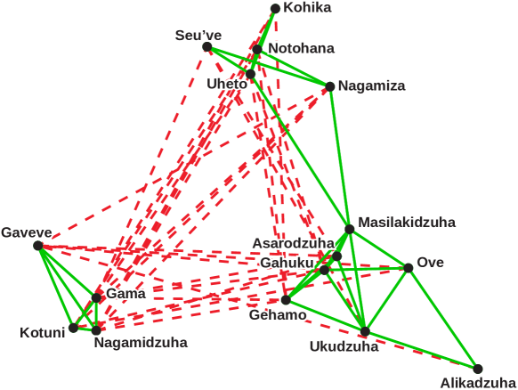
Figure 1: A small example of a signed social network from anthropology: The tribal groups of the Eastern Central Highlands of New Guinea from the study of Read [44]. Individual tribes are the vertices of this network, with friendly relations shown as green edges and antagonistic relations shown as red edges.

In this article, we present ways to measure and exploit structural balance of signed social networks for graph drawing, measuring conflict, detecting communities and predicting links. In particular, we introduce methods based on algebraic graph theory, i.e., the representation of graphs by matrices. In ordinary network analysis applications, algebraic graph theory has the advantage that a large range of powerful algebraic methods become available to analyse networks. In the case of signed networks, an additional advantage is that structural balance, which is inherently a multiplicative construct as illustrated by the rule the enemy of my enemy is my friend, maps in a natural way onto the algebraic representation of networks as matrices. As we will see, this makes not only signed network analysis methods seamlessly take into account structural balance theory, it also simplifies calculation with matrices and vectors, as the multiplication rule is build right into the definition of their operations.

In the rest of article, the individual methods are not presented in order of possible applications, but in order of complexity, building on each other. The breakdown is as follows:

• Section 2 introduces the concept of a signed social network, gives necessary mathematical definitions and presents a set of four signed social networks that are used throughout the paper.

• Section 3 defines structural balance and introduces a basic but novel measure for quantifying it: the signed clustering coefficient.

• Section 4 reviews the problem of drawing signed graphs, and derives from it the signed Laplacian matrix which arises naturally in that context.

• Section 5 gives a proper mathematical definition of the signed Laplacian matrix, and proves its basic properties.

• Section 6 introduces the notion of algebraic conflict, a second way of quantifying structural balance, based on a spectral analysis of the signed Laplacian matrix.

• Section 7 describes the signed graph clustering problem, and shows how its solution leads to another derivation of the signed Laplacian matrix.

• Section 8 reviews the problem of link prediction in signed networks, and shows how it can be solved by the signed resistance distance.

Section 9 concludes the article. This article is partially based on material previously published by the author in conference papers [28, 32, 33, 34, 35].

2 Background: Signed Social Networks

Negative edges can be found in many types of social networks, to model enmity in addition to friendship, distrust in addition to trust, or positive and negative ratings between users. Early uses of signed social networks can be found in anthropology, where negative edges have been used to denote antagonistic relationships between tribes [16]. In this context, the sociological notion of balance is defined as the absence of negative cycles, i.e., the absence of cycles with an odd number of negative edges [9, 17]. Other cases of signed social networks include student relationships [21] and voting processes [36].

Recent studies [18] describe the social network extracted from Essembly, an ideological discussion site that allows users to mark other users as friends, allies and nemeses, and discuss the semantics of the three relation types. These works model the different types of edges by means of three subgraphs. Other recent work considers the task of discovering communities from social networks with negative edges [51].

In trust networks, nodes represent persons or other entities, and links represent trust relationships. To model distrust, negative edges are then used. Work in that field has mostly focused on defining global trust measures using path lengths or adapting PageRank [15, 23, 25, 41, 48].

In applications where users can rate each other, we can model ratings as like and dislike, giving rise to positive and negative edges, for instance on online dating sites [6].

An example of a small signed social network is given by the tribal groups of the Eastern Central Highlands of New Guinea from the study of Read [44] in Figure 1. This dataset describes the relations between sixteen tribal groups of the Eastern Central Highlands of New Guinea [16]. Relations between tribal groups in the Gahuku–Gama alliance structure can be friendly (rova) or antagonistic (hina). In addition, four large signed social networks extracted from the Web will be used throughout the article. All datasets are part of the Koblenz Network Collection [29]. The datasets are summarized in Table 1.

Table 1: The signed social network datasets used in this article. The first four datasets are large; the last one is small and serves as a running example.

Network Type Vertices ($|V|$) Edges ($|E|$) Percent Negative Slashdot Zoo [32] Directed 79,120 515,581 23.9% Epinions [40] Directed 131,828 841,372 14.7% Wikipedia elections [36] Directed 8,297 107,071 21.6% Wikipedia conflicts [5] Undirected 118,100 2,985,790 19.5% Highland tribes [44] Undirected 16 58 50.0%

Definitions

Mathematically, an undirected signed graph can be defined as $G=(V,E,\sigma)$, where $V$ is the vertex set, $E$ is the edge set, and $\sigma:E\rightarrow\{-1,+1\}$ is the sign function [53]. The sign function $\sigma$ assigns a positive or negative sign to each edge. The fact that two edges $u$ and $v$ are adjacent will be denoted by $u\sim v$. The degree of a node $u$ is defined as the number of its neighbors, and can be written as

$$d(u)=\{v\mid u\sim v\}.$$

A directed signed network will be noted as $G=(V,E,\sigma)$, in which $E$ is the set of directed edges (or arcs).

Algebraic Graph Theory

Algebraic graph theory is the branch of graph theory that represents graphs using algebraic structures in order to exploit the powerful methods of algebra in graph theory. The main tool of algebraic graph theory is the representation of graphs as matrices, in particular the adjacency matrix and the Laplacian matrix. In the following, all matrices are real.

Given a signed graph $G=(V,E,\sigma)$, its adjacency matrix $\mathbf{A}\in\mathbb{R}^{|V|\times|V|}$ is defined as

$$\mathbf{A}_{uv} = \left\{\begin{array}[]{ll}\sigma(\{u,v\})&\mathrm{when}\{u,v\}\in E\\ 0&\mathrm{when}\{u,v\}\notin E\end{array}\right.$$

The adjacency matrix is square and symmetric.

The diagonal degree matrix $\mathbf{D}$ of a signed graph is defined using $\mathbf{D}_{uu}=d(u)$. Note that the degrees, and thus the matrix $\mathbf{D}$, is independent of the sign function $\sigma$.

The assumption of structural balance lends itself to using algebraic methods based on the adjacency matrix of a signed network. To see why this is true, consider that the square $\mathbf{A}^{2}$ contains at its entry $(u,v)$ a sum of paths of length two between $u$ and $v$ weighted positively or negatively depending on whether a third positive edge between $u$ and $v$ would lead to a balanced or unbalanced triangle.

Finally, the Laplacian matrix of any graph is defined as $\mathbf{L}=\mathbf{D}-\mathbf{A}$. It is this matrix $\mathbf{L}$ that will play a central role for graph drawing, graph clustering and link prediction.

3 Measuring Structural Balance:
The Signed Clustering Coefficient

In a signed social network, the relationship between two connected nodes can be positive or negative. When looking at groups of three persons, four combinations of positive and negative edges are possible (up to permutations), some being more likely than others. An observation made in actual social groups is that triangles of positive and negative edges tend to be balanced. For instance, a triangle of three positive edges is balanced, as is a triangle of one positive and two negative edges. On the other hand, a triangle of two positive and one negative edge is not balanced. The case of three negative edges can be considered balanced, when considering the three persons as three different groups, or unbalanced, when allowing only two groups.

This characterization of balance can be generalized to the complete signed network, resulting in the following definition:

Definition 1 (Harary, 1953).

A connected signed graph is balanced when its vertices can be partitioned into two groups such that all positive edges connect vertices within the same group, and all negative edges connect vertices of the two different groups.

Figure 3 shows a balanced graph partitioned into two vertex sets. The concept of structural balance can also be illustrated with the phrase the enemy of my enemy is my friend and its permutations.

Equivalently, unbalanced graphs can be defined as those graphs containing a cycle with an odd number of negative edges, as shown in Figure 3. To prove that the balanced graphs are exactly those that do not contain cycles with an odd number of edges, consider that any cycle in a balanced graph has to cross sides an even number of times. On the other hand, any balanced graph can be partitioned into two vertex sets by depth-first traversal while assigning each vertex to a partition such that the balance property is fulfilled. Any inconsistency that arises during such a labeling leads to a cycle with an odd number of negative edges.

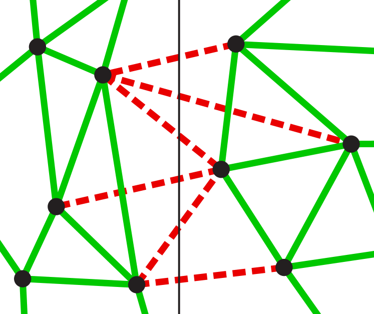
Figure 2: The nodes of a graph without negative cycles can be partitioned into two sets such that all edges inside of each group are positive and all edges between the two groups are negative. We call such a graph balanced.

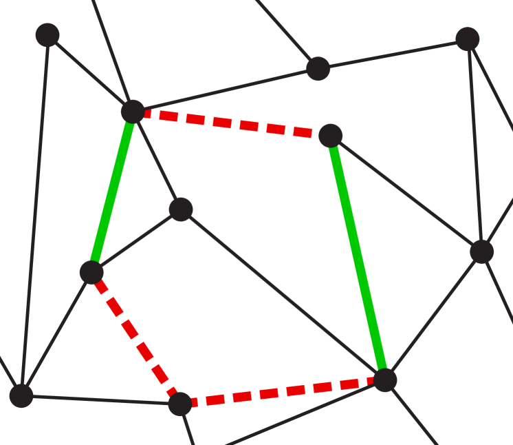
Figure 3: An unbalanced graph contains at least one cycle with an odd number of negative edges. Such a graph cannot be partitioned into two sets with all negative edges across the sets and positive edges within the sets.

In large signed social networks such as those given in Table 1, it cannot be expected that the full network is balanced, since already a single unbalanced triangle makes the full network unbalanced. Instead, we need a measure of balance that characterizes to what extent a signed network is balanced. To that end, we extend a well-establish measure in network analysis, the clustering coefficient, to signed networks, giving the signed clustering coefficient. We also introduce the relative signed clustering coefficient and give the values observed in our example datasets.

The clustering coefficient is a characteristic number of a graph taking values between zero and one, denoting the tendency of the graph nodes to form small clusters. The clustering coefficient was introduced in [49] and an extension for positively weighted edges proposed in [22]. The signed clustering coefficient we define denotes the tendency of small clusters to be balanced, and takes on values between $-1$ and $+1$. The relative signed clustering coefficient will be defined as the quotient between the two.

Figure 4: The four kinds of clustering coefficients. a) Regular clustering coefficient. b) Directed clustering coefficient. c) Signed clustering coefficient. d) Signed directed clustering coefficient. Edge $c$ is counted when edges $a$ and $b$ are present, and for the signed variants, weighted by $\mathrm{sgn}(abc)$.

The clustering coefficient is defined as the proportion of all incident edge pairs that are completed by a third edge to form a triangle. Figure 4 gives an illustration. Given an undirected, unsigned graph $G=(V,E)$ its clustering coefficient is given by

$$c(G) = \frac{\{(u,v,w)\in V^{3}\mid u\sim v\sim w\sim u\}}{\{(u,v,w)\in V^{3}\mid u\sim v\sim w\}}$$ (2)

To extend the clustering coefficient to negative edges, we assume structural balance for two incident signed edges. As shown in Figure 4, an edge with sign $c$ completing two incident edges with signs $a$ and $b$ to form a triangle must fulfill the equation $c=ab$.

$$c_{\mathrm{s}}(G) = \frac{\sum_{u\sim v\sim w\sim u}\sigma(\{u,v\})\sigma(\{v,w\})\sigma(\{w,u\})}{\{u,v,w\in V\mid u\sim v\sim w\}}$$ (3)

Therefore, the signed clustering coefficient denotes to what extent the graph exhibits a balanced structure. In actual signed social networks, we expect it to be positive.

Additionally, we define the relative signed clustering coefficient as the quotient of the signed and unsigned clustering coefficients.

$$S(G)=\frac{c_{s}(G)}{c(G)}=\frac{\sum_{u\sim v\sim w\sim u}\sigma(\{u,v\})\sigma(\{v,w\})\sigma(\{w,u\})}{\{u,v,w\in V\mid u\sim v\sim w\sim u\}}$$ (4)

The relative signed clustering coefficient takes on values between $-1$ and $+1$. It is $+1$ when all triangles are balanced. In networks with negative relative signed clustering coefficients, structural balance does not hold. In fact, the relative signed clustering coefficient is closely related to the number of balanced and unbalanced triangles in a network. If $\Delta^{+}(G)$ is the number of balanced triangles and $\Delta^{-}(G)$ is the number of unbalanced triangles in a signed network $G$, then

$$S(G) = \frac{\Delta^{+}(G)-\Delta^{-}(G)}{\Delta^{+}(G)+\Delta^{-}(G)}.$$

The directed signed clustering coefficient and directed relative signed clustering coefficient can be defined analogously using Expressions (3) and (4). The signed clustering coefficient and relative signed clustering coefficient are zero in random networks, when the sign of edges is distributed equally. The signed clustering coefficients are by definition smaller than their unsigned counterparts.

Table 2: The values for all variants of the clustering coefficient for the example datasets. The directed variants are not computed for the two undirected datasets.

Network	Undirected			Directed
	$c(G)$	$c_{\mathrm{s}}(G)$	$S(G)$	$c(G)$	$c_{\mathrm{s}}(G)$	$S(G)$
Slashdot Zoo	0.0318	0.00607	19.1%	0.0559	0.00918	16.4%
Epinions	0.1107	0.01488	13.4%	0.1154	0.01638	14.2%
Wikipedia elections	0.1391	0.01489	10.9%	0.1654	0.02427	14.7%
Wikipedia conflicts	0.0580	0.03342	57.6%	–	–	–
Highland tribes	0.5271	0.30289	57.5%	–	–	–

Table 2 gives all four variants of the clustering coefficient measured in the example datasets, along with the relative signed clustering coefficients. The high values for the relative clustering coefficients show that our multiplication rule is valid in the examined datasets, and justifies the structural balance approach.

4 Visualizing Structural Balance:
Signed Graph Drawing

To motivate the use of algebraic graph theory based on structural balance, we consider the problem of drawing signed graphs and show how it naturally leads to our definition of the Laplacian matrix for signed graphs. We begin by showing how the signed Laplacian matrix arises naturally in the task of drawing graphs with negative edges when one tries to place each node near to its positive neighbors and opposite to its negative neighbors, extending a standard method of graph drawing in the presence of only positive edges.

The Laplacian matrix turns up in graph drawing when we try to find an embedding of a graph into a plane in a way that adjacent nodes are drawn near to each other [1]. In the literature, signed graphs have been drawn using eigenvectors of the signed adjacency matrix [4]. Instead, our approach consists of using the Laplacian to draw signed graphs, in analogy with the unsigned case. To do this, we will stipulate that negative edges should be drawn as far from each other as possible.

4.1 Unsigned Graphs

We now describe the general method for generating an embedding of the nodes of an unsigned graph into the plane using the Laplacian matrix. Let $G=(V,E)$ be a connected unsigned graph with adjacency matrix $\mathbf{A}$. We want to find a two-dimensional drawing of $G$ in which each vertex is drawn near to its neighbors. This requirement gives rise to the following vertex equation, which states that every vertex is placed at the mean of its neighbors’ coordinates, weighted by the sign of the connecting edges. Let $\mathbf{X}\in\mathbb{R}^{n\times 2}$ be a matrix whose columns are the coordinates of all nodes in the drawing, then we have for each node $u$:

$$\mathbf{X}_{u\bullet}=\left(\sum_{u\sim v}\mathbf{A}_{uv}\right)^{-1}\sum_{u\sim v}\mathbf{A}_{uv}\mathbf{X}_{v\bullet}$$ (5)

Rearranging and aggregating the equation for all $u$ we arrive at

$$\mathbf{D}\mathbf{X}=\mathbf{A}\mathbf{X}$$ (6)

or

$$\mathbf{L}\mathbf{X} = \mathbf{0}.$$

In other words, the columns of $\mathbf{X}$ should belong to the null space of $\mathbf{L}$, which leads to the degenerate solution of $\mathbf{X}_{u\bullet}=\mathbf{1}$ for all $u$, i.e., each $\mathbf{X}_{u\bullet}$ having all components equal, as the all-ones vector $\mathbf{1}$ is an eigenvector of $\mathbf{L}$ with eigenvalue zero. To exclude that solution, we require that the columns $\mathbf{X}$ be orthogonal to $\mathbf{1}$. Additionally, to avoid the degenerate solution $\mathbf{X}_{u\bullet}=\mathbf{X}_{v\bullet}$ for $u\neq v$, we require that all columns of $\mathbf{X}$ be orthogonal. This leads to $\mathbf{X}_{u\bullet}$ being the eigenvectors associated with the two smallest eigenvalues of $\mathbf{L}$ different from zero. This solution results in a well-known satisfactory embedding of unsigned graphs. Such an embedding is related to the resistance distance (or commute-time distance) between nodes of the graph [1].

Note that Equation (6) can also be transformed to $\mathbf{X}=\mathbf{D}^{-1}\mathbf{A}\mathbf{X}$, leading to the eigenvectors of the asymmetric matrix $\mathbf{D}^{-1}\mathbf{A}$. This alternative derivation is not investigated here.

4.2 Signed Graphs

We now extend the graph drawing method described in the previous section to graphs with positive and negative edges. To adapt Expression (5) to negative edges, we interpret a negative edge as an indication that two vertices should be placed on opposite sides of the drawing. Therefore, we take the opposite coordinates $-\mathbf{X}_{v\bullet}$ of vertices $v$ adjacent to $u$ through a negative edge, and then compute the mean, as pictured in Figure 5. We may call this construction antipodal proximity.

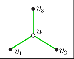
(a) Unsigned graph

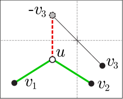
(b) Signed graph

Figure 5: Drawing the vertex $u$ at the mean coordinates of its neighbors $v_{1},v_{2},v_{3}$ by proximity and antipodal proximity. (a) In unsigned graphs, a vertex $u$ is placed at the mean of its neighbors $v_{1},v_{2},v_{3}$. (b) In signed graphs, a vertex $u$ is placed at the mean of its positive neighbors $v_{1},v_{2}$ and antipodal points $-v_{3}$ of its negative neighbors.

This leads to the vertex equation

$$\mathbf{X}_{u\bullet} =\left(\sum_{\{u,v\}\in E}|\mathbf{A}_{ij}|\right)^{-1}\sum_{\{u,v\}\in E}\mathbf{A}_{uv}\mathbf{X}_{v\bullet}$$ (7)

resulting in a signed Laplacian matrix $\mathbf{L}=\mathbf{D}-\mathbf{A}$ in which indeed the definition of the degree matrix $\mathbf{D}_{uu}=\sum_{v}|\mathbf{A}_{uv}|$ leads to the same equation $\mathbf{L}\mathbf{X}=\mathbf{0}$ as in the unsigned case.

As we will see in the next section, $\mathbf{L}$ is always positive-semidefinite, and is positive-definite for graphs that are unbalanced, i.e., graphs that contain cycles with an odd number of negative edges. To obtain a graph drawing from $\mathbf{L}$, we can thus distinguish three cases, assuming that $G$ is connected:

• If all edges are positive, then $\mathbf{L}$ has one eigenvalue zero, and the eigenvectors of the two smallest nonzero eigenvalues can be used for graph drawing.

• If the graph is unbalanced, $\mathbf{L}$ is positive-definite and we can use the eigenvectors of the two smallest eigenvalues as coordinates.

• If the graph is balanced, its spectrum is equivalent to that of the corresponding unsigned Laplacian matrix, up to signs of the eigenvector components. Using the eigenvectors of the two smallest eigenvalues (including zero), we arrive at a graph drawing with all points being placed on two parallel lines, reflecting the perfect 2-clustering present in the graph.

4.3 Synthetic Examples

Figure 6 shows four small synthetic signed graphs drawn using the eigenvectors of three characteristic graph matrices. For each synthetic signed graph, let $\mathbf{A}$ be its adjacency matrix, $\mathbf{L}$ its Laplacian matrix, and $\mathbf{\bar{L}}$ the Laplacian matrix of the corresponding unsigned graph $\bar{G}=|G|$, i.e., the same graph as $G$, only that all edges are positive. For $\mathbf{A}$, we use the eigenvectors corresponding to the two largest absolute eigenvalues. For $\mathbf{L}$ and $\mathbf{\bar{L}}$, we use the eigenvectors of the two smallest nonzero eigenvalues. The small synthetic examples are chosen to display the basic spectral properties of these three matrices. All graphs contain cycles with an odd number of negative edges. Column (a) shows all graphs drawn using the eigenvectors of the two largest eigenvalues of the adjacency matrix $\mathbf{A}$. Column (b) shows the unsigned Laplacian embedding of the graphs by setting all edge weights to $+1$. Column (c) shows the signed Laplacian embedding. The embedding given by the eigenvectors of $\mathbf{A}$ is clearly not satisfactory for graph drawing. As expected, the graphs drawn using the ordinary Laplacian matrix place nodes connected by a negative edge near to each other. The signed Laplacian matrix produces a graph embedding where negative links span large distances across the drawing, as required.

(1)
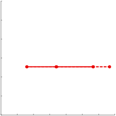
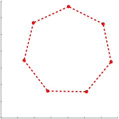
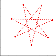
(2)
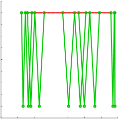
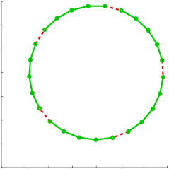
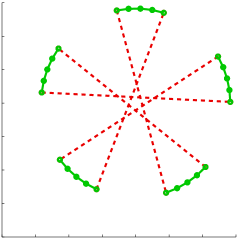
(3)
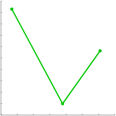
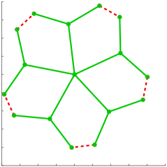
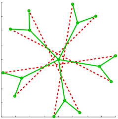
(4)
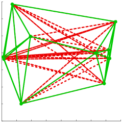
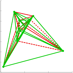
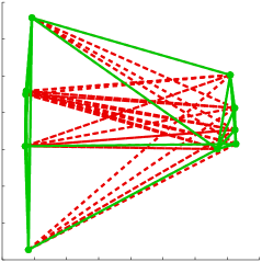
	(a) $\mathbf{A}$	(b) $\mathbf{\bar{L}}$	(c) $\mathbf{L}$

Figure 6: Four small synthetic signed graphs [(1)–(4)] drawn using the eigenvectors of three graph matrices. (a) the adjacency matrix $\mathbf{A}$, (b) the Laplacian $\mathbf{\bar{L}}$ of the underlying unsigned graph $\bar{G}$, (c) the Laplacian $\mathbf{L}$. All graphs shown contain negative cycles, and their signed Laplacian matrices are positive-definite. Positive edges are shown as solid green lines and negative edges as red dashed lines.

Drawing a Balanced Graph

We assume, in the derivation above, that the eigenvectors corresponding to the two smallest eigenvalues of the Laplacian $\mathbf{L}$ should be used for graph drawing. This is true in that it gives the best possible drawing according to the proximity and distance criteria of positive and negative edges. If however the graph is balanced, then, as we will see, the smallest eigenvalue of $\mathbf{L}$ is zero. Unlike the case in unsigned graphs however, the corresponding eigenvector is not constant but contains values $\{\pm 1\}$ describing the split into two partitions. If we use that eigenvector to draw the graph, the resulting drawing will place all vertices on two lines. Such an embedding may be satisfactory in cases where the perfect balance of the graph is to be visualized. If however positive edges among each partition’s vertices are also to be visible, the eigenvector corresponding to the third smallest eigenvalue can be added with a small weight to the first eigenvector, resulting in a two-dimensional representation of a 3-dimensional embedding. The resulting three methods are illustrated in Figure 7.

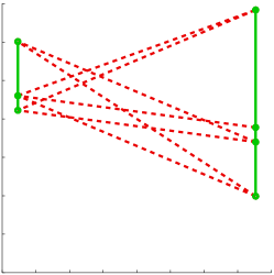
(a) $(\lambda_{1},\lambda_{2})$

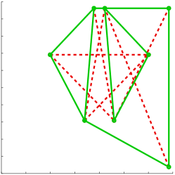
(b) $(\lambda_{2},\lambda_{3})$

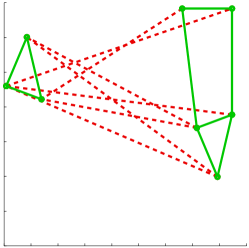
(c) $(\lambda_{1}+0.3\lambda_{3},\lambda_{2})$

Figure 7: Three methods for drawing a balanced signed graph, using a small artificial example network. (a) Using the eigenvector corresponding to the smallest eigenvalue $\lambda_{1}=0$, intra-cluster structure is lost. (b) Ignoring the first eigenvalue misses important information about the clustering. (c) Using a linear combination of both methods gives a good compromise.

In practice, large graphs are almost always unbalanced as shown in Figure 9 and Table 3, and the two smallest eigenvalues give a satisfactory embedding. Figure 8 shows large signed networks drawn using the two eigenvectors of the smallest eigenvalues of the Laplacian matrix $\mathbf{L}$ for three signed networks.

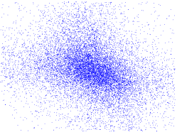
(a) Slashdot Zoo

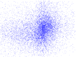
(b) Epinions

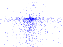
(c) Wikipedia elections

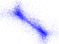
(d) Wikipedia conflicts

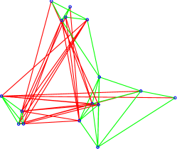
(e) Highland tribes

Figure 8: Signed spectral embedding of networks. For each network, every node is represented as a point whose coordinates are the corresponding values in the eigenvectors of the signed Laplacian $\mathbf{L}$ corresponding to the two smallest eigenvalues. For the Highland tribes network, positive edges are shown in green and negative edges in red. The edges in the other networks are not shown.

5 Capturing Structural Balance:
The Signed Laplacian

The spectrum Laplacian matrix $\mathbf{L}=\mathbf{D}-\mathbf{A}$ of signed networks is studied in [19], where it is established that the signed Laplacian is positive-definite when each connected component of a graph contains a cycle with an odd number of negative edges. Other basic properties of the Laplacian matrix for signed graphs are given in [20].

For an unsigned graph, the Laplacian $\mathbf{L}$ is positive-semidefinite, i.e., it has only nonnegative eigenvalues. In this section, we prove that the Laplacian matrix $\mathbf{L}$ of a signed graph is positive-semidefinite too, characterize the graphs for which it is positive-definite, and give the relationship between the eigenvalue decomposition of the signed Laplacian matrix and the eigenvalue decomposition of the corresponding unsigned Laplacian matrix. Our characterization of the smallest eigenvalue of $\mathbf{L}$ in terms of graph balance is based on [19].

5.1 Positive-semidefiniteness of the Laplacian

A Hermitian matrix is positive-semidefinite when all its eigenvalues are nonnegative, and positive-definite when all its eigenvalues are positive. The Laplacian matrix of an unsigned graph is symmetric and thus Hermitian. Its smallest eigenvalue is zero, and thus the Laplacian of an unsigned graph is always positive-semidefinite but never positive-definite. In the following, we prove that that Laplacian of a signed graph is always positive-semidefinite, and positive-definite when the graph is unbalanced.

Theorem 1.

The Laplacian matrix $\mathbf{L}$ of a signed graph $G=(V,E,\sigma)$ is positive-semidefinite.

Proof.

We write the Laplacian matrix as a sum over the edges of $G$:

$$\mathbf{L}=\sum_{\{u,v\}\in E}\mathbf{L}^{\{u,v\}}$$

where $\mathbf{L}^{\{u,v\}}\in\mathbb{R}^{|V|\times|V|}$ contains the four following nonzero entries:

$$\mathbf{L}^{\{u,v\}}_{uu}=\mathbf{L}^{\{u,v\}}_{vv} = 1$$ (8)

$$\mathbf{L}^{\{u,v\}}_{uv}=\mathbf{L}^{\{u,v\}}_{vu} = -\sigma(\{u,v\})$$

Let $\mathbf{x}\in\mathbb{R}^{|V|}$ be a vertex-vector. By considering the bilinear form $\mathbf{x}^{\mathrm{T}}\mathbf{L}^{\{u,v\}}\mathbf{x}$, we see that $\mathbf{L}^{\{u,v\}}$ is positive-semidefinite:

$$\mathbf{x}^{\mathrm{T}}\mathbf{L}^{\{u,v\}}\mathbf{x} = \mathbf{x}_{u}^{2}+\mathbf{x}_{v}^{2}-2\sigma(\{u,v\})\mathbf{x}_{u}\mathbf{x}_{v}$$

$$= (\mathbf{x}_{u}-\sigma(\{u,v\})\mathbf{x}_{v})^{2}$$

$$\geq 0$$

We now consider the bilinear form $\mathbf{x}^{\mathrm{T}}\mathbf{L}\mathbf{x}$:

$$\mathbf{x}^{\mathrm{T}}\mathbf{L}\mathbf{x}=\sum_{\{u,v\}\in E}\mathbf{x}^{\mathrm{T}}\mathbf{L}^{\{u,v\}}\mathbf{x}\geq 0$$

It follows that $\mathbf{L}$ is positive-semidefinite. ∎

Another way to prove that $\mathbf{L}$ is positive-semidefinite consists of expressing it using the incidence matrix of $G$. Assume that for each edge $\{u,v\}$ an arbitrary orientation is chosen. Then we define the incidence matrix $\mathbf{H}\in\mathbb{R}^{|V|\times|E|}$ of $G$ as

$$\mathbf{H}_{u\{u,v\}} = 1$$

$$\mathbf{H}_{v\{u,v\}} = -\sigma(\{u,v\}).$$

Here, the letter $\mathbf{H}$ is the uppercase greek letter Eta, as used for instance in [14]. We now consider the product $\mathbf{H}\mathbf{H}^{\mathrm{T}}\in\mathbb{R}^{|V|\times|V|}$:

$$(\mathbf{H}\mathbf{H}^{\mathrm{T}})_{uu} = d(u)$$

$$(\mathbf{H}\mathbf{H}^{\mathrm{T}})_{uv} = -\sigma(\{u,v\})$$

for diagonal and off-diagonal entries, respectively. Therefore $\mathbf{H}\mathbf{H}^{\mathrm{T}}=\mathbf{L}$, and it follows that $\mathbf{L}$ is positive-semidefinite. This result is independent of the orientation chosen for $\mathbf{H}$.

5.2 Positive-definiteness of $\mathbf{L}$

We now show that, unlike the ordinary Laplacian matrix, the signed Laplacian matrix is strictly positive-definite for some graphs, including most real-world networks. The theorem presented here can be found in [20], and also follows directly from an earlier result in [52].

As with the ordinary Laplacian matrix, the spectrum of the signed Laplacian matrix of a disconnected graph is the union of the spectra of its connected components. This can be seen by noting that the Laplacian matrix of an unconnected graph has block-diagonal form, with each diagonal entry being the Laplacian matrix of a single component. Therefore, we will restrict the exposition to connected graphs.

Using Definition 1 of structural balance, we can characterize the graphs for which the signed Laplacian matrix is positive-definite.

Theorem 2.

The signed Laplacian matrix of an unbalanced graph is positive-definite.

Proof.

We show that if the bilinear form $\mathbf{x}^{\mathrm{T}}\mathbf{L}\mathbf{x}$ is zero for some vector $\mathbf{x}\neq\mathbf{0}$, then a bipartition of the vertices as described above exists.

Let $\mathbf{x}^{\mathrm{T}}\mathbf{L}\mathbf{x}=0$. We have seen that for every $\mathbf{L}^{\{u,v\}}$ as defined in Equation (8) and any $\mathbf{x}$, $\mathbf{x}^{\mathrm{T}}\mathbf{L}^{\{u,v\}}\mathbf{x}\geq 0$. Therefore, we have for every edge $\{u,v\}$:

$$\mathbf{x}^{\mathrm{T}}\mathbf{L}^{\{u,v\}}\mathbf{x} = 0$$

$$\Leftrightarrow(\mathbf{x}_{u}-\sigma(\{u,v\})\mathbf{x}_{v})^{2} = 0$$

$$\Leftrightarrow\mathbf{x}_{u} = \sigma(\{u,v\})\mathbf{x}_{v}$$

In other words, two components of $\mathbf{x}$ are equal if the corresponding vertices are connected by a positive edge, and opposite to each other if the corresponding vertices are connected by a negative edge. Because the graph is connected, it follows that all $|\mathbf{x}_{u}|$ must be equal. We can exclude the solution $\mathbf{x}_{u}=0$ for all $u$ because $\mathbf{x}$ is not the zero vector. Without loss of generality, we assume that $|\mathbf{x}_{u}|=1$ for all $u$.

Therefore, $\mathbf{x}$ gives a bipartition into vertices with $\mathbf{x}_{u}=+1$ and vertices with $\mathbf{x}_{u}=-1$, with the property that two vertices with the same value of $\mathbf{x}_{u}$ are in the same partition and two vertices with opposite sign of $\mathbf{x}_{u}$ are in different partitions, and therefore $G$ is balanced. Equivalently, the signed Laplacian matrix $\mathbf{L}$ of a connected unbalanced signed graph is positive-definite. ∎

5.3 Balanced Graphs

We now show how the spectrum and eigenvectors of the signed Laplacian of a balanced graph arise from the spectrum and the eigenvalues of the corresponding unsigned graph by multiplication of eigenvector components with $\pm 1$.

Let $G=(V,E,\sigma)$ be a balanced signed graph and $\bar{G}=(V,E)$ the corresponding unsigned graph. Since $G$ is balanced, there is a vector $\mathbf{x}\in\{-1,+1\}^{|V|}$ such that the sign of each edge $\{u,v\}$ is $\sigma(\{u,v\})=\mathbf{x}_{u}\mathbf{x}_{v}$.

Theorem 3.

If $\mathbf{L}$ is the signed Laplacian matrix of the balanced graph $G$ with bipartition $\mathbf{x}$ and eigenvalue decomposition $\mathbf{L}=\mathbf{U}\Lambda\mathbf{U}^{\mathrm{T}}$, then the eigenvalue decomposition of the Laplacian matrix $\mathbf{\bar{L}}$ of $\bar{G}$ of the corresponding unsigned graph $\bar{G}$ of $G$ is given by $\mathbf{\bar{L}}=\mathbf{\bar{U}}\Lambda\mathbf{\bar{U}}^{\mathrm{T}}$ where

$$\mathbf{\bar{U}}_{uk} = \mathbf{x}_{u}\mathbf{U}_{uk}.$$

Proof.

To see that $\mathbf{\bar{L}}=\mathbf{\bar{U}}\Lambda\mathbf{\bar{U}}^{\mathrm{T}}$, note that for diagonal elements, we have $\mathbf{\bar{U}}_{u\bullet}^{\phantom{\mathrm{I}}}\Lambda\mathbf{\bar{U}}_{u\bullet}^{\mathrm{T}}=\mathbf{x}_{u}^{2}\mathbf{U}_{u\bullet}^{\phantom{\mathrm{I}}}\Lambda\mathbf{U}_{u\bullet}^{\mathrm{T}}=\mathbf{U}_{u\bullet}^{\phantom{\mathrm{I}}}\Lambda\mathbf{U}_{u\bullet}^{\mathrm{T}}=\mathbf{L}_{uu}=\mathbf{\bar{L}}_{uu}$. For off-diagonal elements, we have $\mathbf{\bar{U}}_{u\bullet}^{\phantom{\mathrm{I}}}\Lambda\mathbf{\bar{U}}_{v\bullet}^{\mathrm{T}}=\mathbf{x}_{u}\mathbf{x}_{v}\mathbf{U}_{u\bullet}^{\phantom{\mathrm{I}}}\Lambda\mathbf{U}_{v\bullet}^{\mathrm{T}}=\sigma(\{u,v\})\mathbf{L}_{uv}=-\sigma(\{u,v\})\sigma(\{u,v\})=-1=\mathbf{\bar{L}}_{uv}$.

We now show that $\mathbf{\bar{U}}\Lambda\mathbf{\bar{U}}^{\mathrm{T}}$ is an eigenvalue decomposition of $\mathbf{\bar{L}}$ by showing that $\mathbf{\bar{U}}$ is orthogonal. To see that the columns of $\mathbf{\bar{U}}$ are indeed orthogonal, note that for any two column indexes $k\neq l$, we have $\mathbf{\bar{U}}_{\bullet k}^{\mathrm{T}}\mathbf{\bar{U}}_{\bullet l}^{\phantom{\mathrm{I}}}=\sum_{u\in V}\mathbf{\bar{U}}_{uk}\mathbf{\bar{U}}_{ul}=\sum_{u\in V}\mathbf{x}_{u}^{2}\mathbf{U}_{uk}\mathbf{U}_{ul}=\mathbf{U}_{\bullet k}^{\mathrm{T}}\mathbf{U}_{\bullet l}^{\phantom{\mathrm{I}}}=0$ because $\mathbf{U}$ is orthogonal. Changing signs in $\mathbf{U}$ does not change the norm of each column vector, and thus $\mathbf{\bar{L}}=\mathbf{\bar{U}}\Lambda\mathbf{\bar{U}}^{\mathrm{T}}$ is the eigenvalue decomposition of $\mathbf{\bar{L}}$. ∎

As shown in Section 5.2, the Laplacian matrix of an unbalanced graph is positive-definite and therefore its spectrum is different from that of the corresponding unsigned graph. Aggregating Theorems 2 and 3, we arrive at the main result of this section.

Theorem 4.

The Laplacian matrix of a connected signed graph is positive-definite if and only if the graph is unbalanced.

Proof.

From Theorem 2 we know that every unbalanced connected graph has a positive-definite Laplacian matrix. Theorem 3 implies that every balanced graph has the same Laplacian spectrum as its corresponding unsigned graph. Since the unsigned Laplacian is always singular, the signed Laplacian of a balanced graph is also singular. Together, these imply that the Laplacian matrix of a connected signed graph is positive-definite if and only if the graph is unbalanced. ∎

For a general signed graph that need not be connected, we can therefore make the following statement: The multiplicity of the eigenvalue zero equals the number of balanced connected components in $G$ [14].

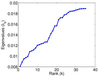
(a) Slashdot Zoo

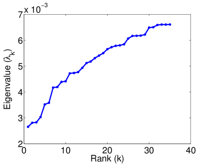
(b) Epinions

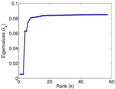
(c) Wikipedia elections

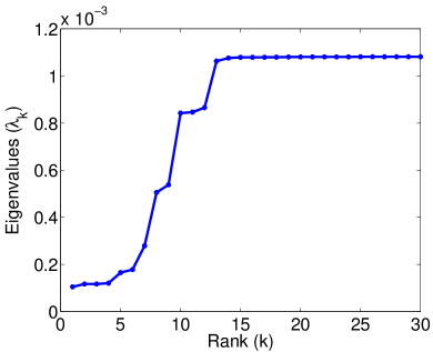
(d) Wikipedia conflicts

Figure 9: The Laplacian spectra of three signed networks. These plots show the eigenvalues $\lambda_{1}\leq\lambda_{2}\leq\cdots$ of the Laplacian matrix $\mathbf{L}$.

The spectra of several large unipartite signed networks are plotted in Figure 9. We can observe that in all cases, the smallest eigenvalue is larger than zero, implying, as expected, that these graphs are unbalanced.

6 Measuring Structural Balance 2:
Algebraic Conflict

The smallest eigenvalue of the Laplacian $\mathbf{L}$ of a signed graph is zero when the graph is balanced, and larger otherwise. We derive from this that the smallest Laplacian eigenvalue characterizes the amount of conflict present in the graph. We will call this number the algebraic conflict of the graph and denote it $\xi$.

Let $G=(V,E,\sigma)$ be a connected signed graph with adjacency matrix $\mathbf{A}$, degree matrix $\mathbf{D}$ and Laplacian $\mathbf{L}=\mathbf{D}-\mathbf{A}$. Let $\lambda_{1}\leq\lambda_{2}\leq\cdots\leq\lambda_{|V|}$ be the eigenvalues of $\mathbf{L}$. Because $\mathbf{L}$ is positive-semidefinite (Theorem 1), we have $\lambda_{1}\geq 0$. According to Theorem 2, $\lambda_{1}$ is zero exactly when $G$ is balanced. Therefore, the value $\lambda_{1}$ can be used as an invariant of signed graphs that characterizes the conflict due to unbalanced cycles, i.e., cycles with an odd number of negative edges. We will call $\xi=\lambda_{1}$ the algebraic conflict of the network. The number $\xi$ is discussed in [19] and [35], without being given a specific name.

The algebraic conflict $\xi$ for our signed network datasets is compared in Table 3. All these large networks are unbalanced, and we can for instance observe that the social networks of the Slashdot Zoo and Epinions are more balanced than the election network of Wikipedia.

Table 3: The algebraic conflict $\xi$ for several signed unipartite networks. Smaller values indicate a more balanced network; larger values indicate more conflict.

Network	$\xi$
Slashdot Zoo	0.008077
Epinions	0.002657
Wikipedia elections	0.005437
Wikipedia conflicts	0.0001050
Highland tribes	0.7775

Figure 10 plots the algebraic conflict of the signed networks against the relative signed clustering coefficient The number of signed datasets is small, and thus we cannot make out a correlation between the two measures, although the data is consistent with a negative between the two measures, as expected.

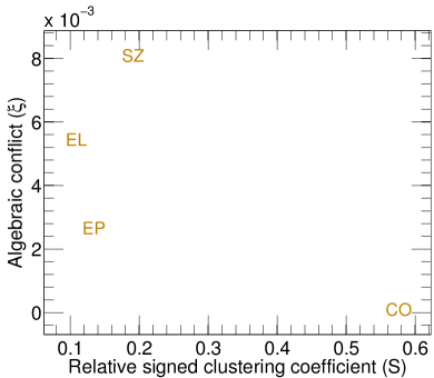
Figure 10: Scatter plot of the two measures of balance and conflict for the four signed social networks: The relative signed clustering coefficient $S$ and the algebraic conflict $\xi$. (SZ: Slashdot Zoo, EP: Epinions, EL: Wikipedia elections, CO: Wikipedia conflict)

Monotonicity

From the definition of the algebraic conflict $\xi$, we can derive a simple theorem stating that adding an edge of any weight to a signed graph can only increase the algebraic conflict, not decrease it.

Theorem 5.

Let $G=(V,E,\sigma)$ be a signed graph and $u,v\in V$ two vertices such that $\{u,v\}\notin E$, and $\xi$ the algebraic of $G$. Furthermore, let $G^{\prime}=(V,E\cup\{u,v\},\sigma^{\prime})$ with $\sigma^{\prime}(e)=\sigma(e)$ when $e\in E$ and $\sigma(\{u,v\})=\sigma$ otherwise be the graph $G$ to which an edge with sign $\sigma$ has been added. Then, let $\xi^{\prime}$ be the algebraic conflict of $G^{\prime}$. Then, $\xi\leq\xi^{\prime}$.

Proof.

We make use of a theorem stated for instance in [50, p. 97]. This theorem states that when adding a positive-semidefinite matrix $\mathbf{E}$ of rank one to a given symmetric matrix $\mathbf{X}$ with eigenvalues $\lambda_{1}\leq\lambda_{2}\leq\cdots\leq\lambda_{n}$, the new matrix $\mathbf{X}^{\prime}=\mathbf{X}+\mathbf{E}$ has eigenvalues $\lambda^{\prime}_{1}\leq\lambda^{\prime}_{2}\leq\cdots\leq\lambda^{\prime}_{n}$ which interlace the eigenvalues of $\mathbf{X}$:

$$\lambda_{1}^{\phantom{{}^{\prime}}}\leq\lambda^{\prime}_{1}\leq\lambda_{2}^{\phantom{{}^{\prime}}}\leq\lambda^{\prime}_{2}\leq\cdots\leq\lambda_{n}^{\phantom{{}^{\prime}}}\leq\lambda^{\prime}_{n}$$

The Laplacian $\mathbf{L}^{\prime}$ of $G^{\prime}$ can be written as $\mathbf{L}^{\prime}=\mathbf{L}+\mathbf{E}$, where $\mathbf{E}\in\mathbb{R}^{|V|\times|V|}$ is the matrix defined by $\mathbf{E}_{uu}=\mathbf{E}_{vv}=1$ and $\mathbf{E}_{uv}=\mathbf{E}_{vu}=-\sigma$, and $\mathbf{E}_{uv}=0$ for all other entries. Then let $\mathbf{e}\in\mathbb{R}^{|V|}$ be the vector defined by $\mathbf{e}_{u}=1$, $\mathbf{e}_{v}=-\sigma$ and $\mathbf{e}_{w}=0$ for all other entries. We have $\mathbf{E}=\mathbf{e}\mathbf{e}^{\mathrm{T}}$, and therefore $\mathbf{E}$ is positive-semidefinite.

Now, due to the interlacing theorem mentioned above, adding a positive-semidefinite matrix to a given symmetric matrix can only increase each eigenvalue, but not decrease it. Therefore, $\lambda_{1}\leq\lambda^{\prime}_{1}$, and thus $\xi\leq\xi^{\prime}$. ∎

We have thus proved that adding an edge of any sign to a signed network can only increase the algebraic conflict, not decrease it. It also follows that removing an edge of any sign from a signed network can decrease the algebraic conflict or leave it unchanged, but not increase it.

7 Maximizing Structural Balance:
Signed Spectral Clustering

One of the main application areas of the graph Laplacian are clustering problems. In spectral clustering, the eigenvectors of matrices associated with a graph are used to partition the vertices of the graph into well-connected groups. In this section, we show that in a signed graph, the spectral clustering problem corresponds to finding clusters of vertices connected by positive edges, but not connected by negative edges.

Spectral clustering algorithms are usually derived by formulating a minimum cut problem which is then relaxed [8, 39, 42, 43, 46]. The choice of the cut function results in different spectral clustering algorithms. In all cases, the vertices of a given graph are mapped into the space spanned by the eigenvectors of a matrix associated with the graph.

In this section we derive a signed extension of the ratio cut, which leads to clustering with the signed Laplacian $\mathbf{L}$. We restrict our proofs to the case of clustering vertices into two groups; higher-order clusterings can be derived analogously.

7.1 Unsigned Graphs

We first review the derivation of the ratio cut in unsigned graphs. Let $G=(V,E)$ be an unsigned graph with adjacency matrix $\mathbf{A}$. A cut of $G$ is a partition of the vertices $V$ into the nonempty sets $V_{1}$ and $V_{2}$, whose weight is given by

$$\mathrm{Cut}(V_{1},V_{2})=|\{\{u,v\}\in E\mid u\in V_{1},v\in V_{2}\}|.$$

The cut measures how well two clusters are connected. Since we want to find two distinct groups of vertices, the cut must be minimized. Minimizing $\mathrm{Cut}(V_{1},V_{2})$ however leads in most cases to solutions separating very few vertices from the rest of the graph. Therefore, the cut is usually divided by the size of the clusters, giving the ratio cut:

$$\mathrm{RatioCut}(V_{1},V_{2})=\left(\frac{1}{|V_{1}|}+\frac{1}{|V_{2}|}\right)\mathrm{Cut}(V_{1},V_{2})$$

To get a clustering, we then solve the following optimization problem:

$$\min_{V_{1}\subset V}\quad\mathrm{RatioCut}(V_{1},V\setminus V_{1})$$

Let $V_{2}=V\setminus V_{1}$. Then this problem can be solved by expressing it in terms of the characteristic vector $\mathbf{x}\in\mathbb{R}^{|V|}$ of $V_{1}$ defined by:

$$\mathbf{x}_{u}=\left\{\begin{array}[]{ll}+\sqrt{|V_{2}|/|V_{1}|}&\textnormal{ if }u\in V_{1}\\ -\sqrt{|V_{1}|/|V_{2}|}&\textnormal{ if }u\in V_{2}\end{array}\right.$$ (12)

We observe that $\mathbf{x}\mathbf{L}\mathbf{x}^{\mathrm{T}}=2|V|\cdot\mathrm{RatioCut}(V_{1},V_{2})$, and that $\sum_{u}\mathbf{x}_{u}=0$, i.e., $\mathbf{x}$ is orthogonal to the constant vector. Denoting by $\mathcal{X}$ the vectors $\mathbf{x}$ of the form given in Equation (12) we have

$$\min_{\mathbf{x}\in\mathbb{R}^{|V|}} \mathbf{x}\mathbf{L}\mathbf{x}^{\mathrm{T}}$$ (13)

$$\mathrm{s.t.} \mathbf{x}\cdot\mathbf{1}=0,\mathbf{x}\in\mathcal{X}$$

This can be relaxed by removing the constraint $\mathbf{x}\in\mathcal{X}$, giving as solution the eigenvector of $\mathbf{L}$ having the smallest nonzero eigenvalue [39].

7.2 Signed Graphs

We now give a derivation of the ratio cut for signed graphs. Let $G=(V,E,\sigma)$ be a signed graph with adjacency matrix $\mathbf{A}$. We write $\mathbf{A}^{\oplus}$ and $\mathbf{A}^{\ominus}$ for the adjacency matrices containing only the positive and negative edges. In other words, $\mathbf{A}^{\oplus}_{uv}=\max(0,\mathbf{A}_{uv})$, $\mathbf{A}^{\ominus}_{uv}=\max(0,-\mathbf{A}_{uv})$ and $\mathbf{A}=\mathbf{A}^{\oplus}-\mathbf{A}^{\ominus}$.

For convenience we define positive and negative cuts that only count positive and negative edges respectively:

$$\mathrm{Cut}^{\oplus}(V_{1},V_{2}) = \sum_{u\in V_{1},v\in V_{2}}\mathbf{A}^{\oplus}_{uv}$$

$$\mathrm{Cut}^{\ominus}(V_{1},V_{2}) = \sum_{u\in V_{1},v\in V_{2}}\mathbf{A}^{\ominus}_{uv}$$

In these definitions, we allow $V_{1}$ and $V_{2}$ to be overlapping. For a vector $\mathbf{x}\in\mathbb{R}^{|V|}$, we consider the bilinear form $\mathbf{x}^{\mathrm{T}}\mathbf{L}\mathbf{x}$. As shown in Equation (5.1), this can be written in the following way:

$$\mathbf{x}^{\mathrm{T}}\mathbf{L}\mathbf{x}=\sum_{\{u,v\}\in E}(\mathbf{x}_{u}-\sigma(\{u,v\})\mathbf{x}_{v})^{2}$$

For a given partition $V=V_{1}\cup V_{2}$, let $\mathbf{x}\in\mathbb{R}^{|V|}$ be the following vector:

$$\mathbf{x}_{u}=\left\{\begin{array}[]{ll}+\frac{1}{2}\left(\sqrt{\frac{|V_{1}|}{|V_{2}|}}+\sqrt{\frac{|V_{2}|}{|V_{1}|}}\right)&\textnormal{ if }u\in V_{1}\\ -\frac{1}{2}\left(\sqrt{\frac{|V_{1}|}{|V_{2}|}}+\sqrt{\frac{|V_{2}|}{|V_{1}|}}\right)&\textnormal{ if }u\in V_{2}\end{array}\right.$$ (16)

The corresponding bilinear form then becomes:

$$\mathbf{x}^{\mathrm{T}}\mathbf{L}\mathbf{x} = \sum_{\{u,v\}\in E}\left(\mathbf{x}_{u}-\sigma(\{u,v\})\mathbf{x}_{v}\right)^{2}$$

$$= |V|\left(\frac{1}{|V_{1}|}+\frac{1}{|V_{2}|}\right)\left(2\cdot\mathrm{Cut}^{\oplus}(V_{1},V_{2})+\mathrm{Cut}^{\ominus}(V_{1},V_{1})+\mathrm{Cut}^{\ominus}(V_{2},V_{2})\right)$$

This leads us to define the following signed cut of $(V_{1},V_{2})$:

$$\mathrm{SignedCut}(V_{1},V_{2}) = \mathrm{Cut}^{\oplus}(V_{1},V_{2})+\frac{1}{2}\left(\mathrm{Cut}^{\ominus}(V_{1},V_{1})+\mathrm{Cut}^{\ominus}(V_{2},V_{2})\right)$$

and to define the signed ratio cut as follows:

$$\mathrm{SignedRatioCut}(V_{1},V_{2})=\left(\frac{1}{|V_{1}|}+\frac{1}{|V_{2}|}\right)\mathrm{SignedCut}(V_{1},V_{2})$$

Therefore, the following minimization problem solves the signed clustering problem:

$$\min_{V_{1}\subset V}\quad\mathrm{SignedRatioCut}(V_{1},V\setminus V_{1})$$

We can now express this minimization problem using the signed Laplacian, where $\mathcal{X}$ denotes the set of vectors of the form given in Equation (16):

$$\min_{\mathbf{x}\in\mathbb{R}^{|V|}} \quad\mathbf{x}\mathbf{L}\mathbf{x}^{\mathrm{T}}$$

$$\mathrm{s.t.} \quad\mathbf{x}\in\mathcal{X}$$

Note that we lose the orthogonality of $\mathbf{x}$ to the constant vector. This can be explained by the fact that if $G$ contains negative edges, the smallest eigenvector can always be used for clustering: If $G$ is balanced, the smallest eigenvalue is zero and its eigenvector equals $(\pm 1)$ and gives the two clusters separated by negative edges. If $G$ is unbalanced, then the smallest eigenvalue of $\mathbf{L}$ is larger than zero by Theorem 2, and the constant vector is not an eigenvalue.

The signed cut $\mathrm{SignedCut}(V_{1},V_{2})$ counts the number of positive edges that connect the two groups $V_{1}$ and $V_{2}$, and the number of negative edges that remain in each of these groups. Thus, minimizing the signed cut leads to clusterings where two groups are connected by few positive edges and contain few negative edges inside each group. This signed ratio cut generalizes the ratio cut of unsigned graphs and justifies the use of the signed Laplacian $\mathbf{L}$ and its particular definition for spectral clustering of signed graphs.

7.3 Signed Clustering using Other Matrices

When instead of normalizing with the number of vertices $|V_{1}|$ we normalize with the number of edges $\mathrm{vol}(V_{1})$, the result is a spectral clustering algorithm based on the eigenvectors of $\mathbf{D}^{-1}\mathbf{A}$ introduced by Shi and Malik [46]. The cuts normalized by $\mathrm{vol}(V_{1})$ are called normalized cuts. In the signed case, the eigenvectors of $\mathbf{D}^{-1}\mathbf{A}$ lead to the signed normalized cut:

$$\mathrm{SignedNormalizedCut}(V_{1},V_{2}) = \left(\frac{1}{\mathrm{vol}(V_{1})}+\frac{1}{\mathrm{vol}(V_{2})}\right)\mathrm{SignedCut}(V_{1},V_{2})$$

A similar derivation can be made for normalized cuts based on $\mathbf{N}=\mathbf{D}^{-1/2}\mathbf{A}\mathbf{D}^{-1/2}$, generalizing the spectral clustering method of Ng, Jordan and Weiss [43]. The dominant eigenvector of the signed adjacency matrix $\mathbf{A}$ can also be used for signed clustering [2]. As in the unsigned case, this method is not suited for very sparse graphs, and does not have an interpretation in terms of cuts.

Example

As an application of signed spectral clustering to real-world data, we cluster the tribes in the Highland tribes network. The resulting graph contains cycles with an odd number of negative edges, and therefore its signed Laplacian matrix is positive-definite. We use the eigenvectors of the two smallest eigenvalues ($\lambda_{1}=1.04$ and $\lambda_{2}=2.10$) to embed the graph into the plane. The result is shown in Figure 11. We observe that indeed the positive (green) edges are short, and the negative (red) edges are long. Looking at only the positive edges, the drawing makes the two connected components easy to see. Looking at only the negative edges, we recognize that the tribal groups can be clustered into three groups, with no negative edges inside any group. These three groups correspond indeed to a higher-order grouping in the Gahuku–Gama society [16].

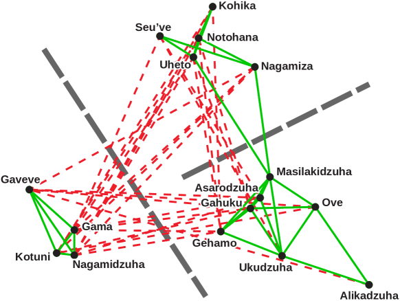
Figure 11: The tribal groups of the Eastern Central Highlands of New Guinea from the study of Read [44] clustered using eigenvectors of the Laplacian matrix. The three higher-order groups as described by Hage and Harary [16] are linearly separable.

8 Predicting Structural Balance:
Signed Resistance Distance

In the field of network analysis, one of the major applications consists in predicting the state of an evolving network in the future. When considering only the network structure, the corresponding learning problem is the link prediction problem. In this section, we will show that a certain class of link prediction algorithms based on algebraic graph theory are particularly suited to signed social networks, since they fulfill three natural requirements that a link prediction method should follow. We will state the three conditions, and then present two algebraic link prediction methods: the exponential of the adjacency matrix and the signed resistance distance. We then finally evaluate the methods on the task of link prediction.

First however, let us give the correct terminology and define the link prediction problem for unsigned and signed social networks. Although we state both problems in terms of social networks, both problems can be extended to other networks.

Actual social networks are not static graphs, but dynamic systems in which nodes and edges are added and removed continuously. The main type of change being the addition of edges, i.e., the appearance of a new tie. Predicting such ties is a common task. For instance, social networking sites try to predict who users are likely to already know in order to give good friend recommendations. Let $G=(V,E)$ be an unsigned social network. The link prediction then consists of predicting new edges in that network, a link prediction algorithm is thus a function mapping a given network to edge predictions. In this work, we will express link prediction functions algebraically as a map from the $|V|\times|V|$ adjacency matrix of a network to another $|V|\times|V|$ matrix containing link prediction scores. The semantics of these scores is that higher values denote a higher likelihood of link formation. Apart from that, we do not put any other constraint on link prediction scores. In particular, link prediction scores do not have to be nonnegative, or restricted to the range $[0,1]$.

In the case of signed social networks, the link prediction problem is usually restricted to predicting positive edges. This is easily motivated by the example of a social recommender system, which should recommend friends and not enemies. Thus, the link prediction problem for signed networks can be formalized in the same fashion as for unsigned networks, by a function from the space of adjacency matrices (containing positive and negative entries) to the space of score matrices. A link prediction function $f$ for signed networks will thus be denoted as follows:

$$f:\{-1,0,+1\}^{|V|\times|V|}\rightarrow\mathbb{R}^{|V|\times|V|}$$

A note is in order about the related problem of link sign prediction. In the problem of link sign prediction, a signed (social) network is given, along with a set of unweighted edges, and the goal is the predict the sign of the edges [32, 37]. This problem is different from the link prediction problem in that for each given edge, it is known that the edge is part of the network, and only its sign must be predicted. By contrast, the link prediction problem assumes no knowledge about the network and consists in finding the positive edges.

Requirements of a Link Prediction Function

The structure of the link prediction problem implies two requirements for a link prediction function, in relation with paths connecting any two nodes. In addition, the presence of negative edges implies a third requirement, in relation to the edge signs in paths connecting two nodes.

Let $V$ be a fixed set of vertices, and $G_{1}=(V,E_{1})$ and $G_{2}=(V,E_{2})$ two unsigned networks with the same vertex sets. Let $u,v\in V$ be two vertices and $f$ a link prediction function. Then, compare the set set of paths connecting the vertices $u$ and $v$, both in $G_{1}$ and in $G_{2}$. Two requirements should be fulfilled by $f$:

• Path counts: If more paths between $u$ and $v$ are present in $G_{1}$ than $G_{2}$, than $f$ should return a higher score for the pair $(u,v)$ in $G_{1}$ than in $G_{2}$.

• Path lengths: If paths between $u$ and $v$ are longer in $G_{1}$ than in $G_{2}$, then $f$ should return a lower score for the pair $(u,v)$ in $G_{1}$ than in $G_{2}$.

In addition, the following requirement can be formulated for signed networks. In this requirement, we will refer to a path as positive when it contains an even number of negative edges and as negative when it contains an odd number of negative edges.

• Path signs: If paths between $u$ and $v$ are more often positive in $G_{1}$ than in $G_{2}$, than $f$ should return a higher score for the pair $(u,v)$ in $G_{1}$ than in $G_{2}$.

These three requirements are fulfilled by several link prediction functions, of which we review one and introduce another in the following.

8.1 Signed Matrix Exponential

Let $G=(V,E,\sigma)$ be a signed network with adjacency matrix $\mathbf{A}$. Its exponential is then defined as

$$e^{\alpha\mathbf{A}} = \mathbf{I}+\mathbf{A}+\frac{1}{2}\mathbf{A}^{2}+\frac{1}{6}\mathbf{A}^{3}+\cdots$$

This exponential with the parameter $\alpha>0$ is a suitable link prediction function for signed networks as it can be expressed as a sum over all paths between any two nodes. Let $P_{G}(u,v,k)$ be the set of paths of length $k$ in the graph $G$. In this definition, we allow a path to cross a single vertex multiple times, and set the length of a path as being the number of edges it contains. Furthermore, let

$$(v_{0},v_{1},\ldots,v_{k})\in P_{G}(u,v,k)$$

with $u=v_{0}$ and $v=v_{k}$. Then, any power of $\mathbf{A}$ can be expressed as

$$(\mathbf{A}^{k})_{uv} = \sum_{(v_{0},\ldots,v_{k})\in P_{G}(u,v,k)}\prod_{i=1}^{k}\sigma(\{v_{i-1},v_{i}\}).$$

In other words, the $k$^th power of the adjacency matrix equals a sum over all paths of length $k$, weighted by the product of their edge signs. This leads to the following expression for the matrix exponential:

$$(e^{\alpha\mathbf{A}})_{uv} = \sum_{k=0}^{\infty}\frac{\alpha^{k}}{k!}\sum_{(v_{0},\ldots,v_{k})\in P_{G}(u,v,k)}\prod_{i=1}^{k}\sigma(\{v_{i-1},v_{i}\}).$$

In other words, the matrix exponential is a sum over all paths between any two nodes, weighted by the function $\alpha^{k}/k!$ of their path length. This implies that the matrix exponential is a suitable link sign prediction function for signed networks, since it fulfills all three requirements:

• Path counts: The exponential function is a sum over paths and thus counts paths.

• Path lengths: The function $\alpha^{k}/k!$ is decreasing in $k$, for suitably small values of $\alpha$.

• Path signs: Signs are taken into account by multiplication.

Thus, the exponential of the adjacency matrix is a link prediction function for signed networks.

Other, similar functions can be constructed, for instance the function $(\mathbf{I}-\alpha\mathbf{A})^{-1}$ is known as the Neumann kernel, in which $\alpha$ is chosen such that $\alpha^{-1}>|\lambda_{1}|$, $|\lambda_{1}|$ being $\mathbf{A}$’s largest absolute eigenvalue, or equivalently the graph’s spectral norm [24].

Both the matrix exponential and the Neumann kernel can be applied to the normalized adjacency matrix $\mathbf{N}=\mathbf{D}^{-1/2}\mathbf{A}\mathbf{D}^{-1/2}$, in which each edge $\{u,v\}$ is weighted by $\sqrt{d(u)d(v)}$, i.e., the geometric mean of the degrees of $u$ and $v$. The rationale behind this normalization is to count a connection as less important if it is one of many that attaches to a node.

8.2 Signed Resistance Distance

The resistance distance is a metric defined on vertices of a graph inspired from electrical resistance networks. When an electrical current is applied to an electrical network of resistors, the whole network acts as a single resistor whose resistance is a function of the individual resistances. In such an electrical network, any two nodes of the network can be taken as the endpoint of the total resistance, giving a function defined between every pair of nodes. As shown in [26], this function is a metric, usually called the resistance distance.

Intuitively, two nodes further apart are separated by a greater equivalent resistance, while nodes closer to each other lead to a small resistance distance. This distance function has been used before to perform collaborative filtering [11, 12, 13], and it fulfills the first two of our assumptions, when actual edge weights are interpreted as inverse resistances, i.e., conductances:

• Path counts: Parallel resistances are inverse-additive, and parallel conductances are additive.

• Path lengths: Resistances in series are additive and conductances in series inverse-additive.

As the resistance distance by default only applies to nonnegative values, previous works use it on nonnegative data, such as unsigned social networks or document view counts. In the presence of signed edges, the resistance distance can be extended by the following formalism, which fulfills the third requirement on path signs. A positive electrical resistance indicates that the potentials of two connected nodes will tend to each other: The smaller the resistance, the more both potentials approach each other. Therefore, a positive edge can be represented as a unit resistor. If an edge is negative, we can interpret the connection as consisting of a unit resistor in series with an inverting amplifier that guarantees its ends to have opposite voltage, as depicted in Figure 12. In other words, two nodes connected by a negative edge will tend to opposite voltages.

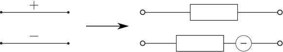
Figure 12: Interpretation of positive and negative edges as electrical components. An edge with a negative weight is interpreted as a positive resistor in series with an inverting component (shown as $\circleddash$).

Thus, a positive edge can be modeled by a unit resistor and a negative edge can be modeled by a unit resistor in series with a (hypothetical) electrical component that assures its ends have opposite electrical potential. Note that the absence of an edge is modeled by the absence of a resistor, which is equivalent to a resistor with infinite resistance. Thus, actual edge weights and scores correspond not to resistances, but to inverse resistance, i.e., conductances.

We now establish a closed-form expression giving the resistance distance between all node pairs based on [26].

Definitions

The following notation is used.

• $\mathbf{J}_{uv}$ is the current flowing through the oriented edge $(u,v)$. $\mathbf{J}$ is skew-symmetric: $\mathbf{J}_{uv}=-\mathbf{J}_{vu}$.

• $\mathbf{v}_{u}$ is the electric potential at node $u$. Potentials are defined up to an additive constant.

• $\mathbf{R}_{uv}$ is the resistance value of edge $(u,v)$. Note that $\mathbf{R}_{uv}=\mathbf{R}_{vu}$.

In electrical networks, the current entering a node must be equal to the current leaving that node. This relation is known as Kirchhoff’s law, and can be expressed as $\sum_{v\sim u}\mathbf{J}_{uv}=0$ for all $u\in V$. We assume that a current $j$ will be flowing through the network from vertex $a$ to vertex $b$, and therefore we have

$$\sum_{(v,a)}\mathbf{J}_{av} = j,$$

$$\sum_{(v,b)}\mathbf{J}_{bv} = -j.$$

Using the identity matrix $\mathbf{I}$, we express these relations as

$$\sum_{(v,u)}\mathbf{J}_{uv}=j(\mathbf{I}_{ua}-\mathbf{I}_{ub})$$ (17)

The relation between currents and potentials is given by Ohm’s law: $\mathbf{v}_{u}-\mathbf{v}_{v}=\mathbf{R}_{uv}\mathbf{J}_{uv}$ for all edges $(u,v)$.

We will now show that the equivalent resistance $\mathbf{\bar{R}}_{ab}$ between $a$ and $b$ in the network can be expressed in terms of the graph Laplacian $\mathbf{L}$ as

$$\mathbf{\bar{R}}_{ab} = (\mathbf{I}_{a\bullet}-\mathbf{I}_{b\bullet})\mathbf{L}^{+}(\mathbf{I}_{a\bullet}-\mathbf{I}_{b\bullet})^{\mathrm{T}},$$

$$= \mathbf{L}^{+}_{aa}+\mathbf{L}^{+}_{bb}-\mathbf{L}^{+}_{ab}-\mathbf{L}^{+}_{ba},$$

where $\mathbf{L}^{+}$ is the Moore–Penrose pseudoinverse of $\mathbf{L}$ [26].

The proof follows from recasting Equation (17) as:

$$\sum_{(v,u)}\frac{1}{\mathbf{R}_{uv}}(\mathbf{v}_{u}-\mathbf{v}_{v}) =j(\mathbf{I}_{ua}-\mathbf{I}_{ub})$$

Combining over all $u\in V$:

$$\mathbf{D}\mathbf{v}-\mathbf{A}\mathbf{v} = j(\mathbf{I}_{a\bullet}-\mathbf{I}_{b\bullet})$$

$$\mathbf{L}\mathbf{v} = j(\mathbf{I}_{a\bullet}-\mathbf{I}_{b\bullet})$$

Let $\mathbf{L}^{+}$ be the Moore–Penrose pseudoinverse of $\mathbf{L}$, then because $\mathbf{v}$ is contained in the row space of $\mathbf{L}$ [26], we have $\mathbf{L}^{+}\mathbf{L}\mathbf{v}=\mathbf{v}$, and we get

$$\mathbf{v} = \mathbf{L}^{+}j(\mathbf{I}_{a\bullet}-\mathbf{I}_{b\bullet})$$

Which finally gives the equivalent resistance between $a$ and $b$ as

$$\mathbf{\tilde{R}}_{ab} = (\mathbf{v}_{a}-\mathbf{v}_{b})/j$$

$$= (\mathbf{I}_{a\bullet}-\mathbf{I}_{b\bullet})^{\mathrm{T}}\mathbf{v}/j$$

$$= (\mathbf{I}_{a\bullet}-\mathbf{I}_{b\bullet})^{\mathrm{T}}\mathbf{L}^{+}(\mathbf{I}_{a\bullet}-\mathbf{I}_{b\bullet})$$

A symmetry argument shows that $\mathbf{\tilde{R}}_{ab}=\mathbf{\tilde{R}}_{ba}$ as expected. As shown in [26], $\mathbf{\tilde{R}}$ is a metric.

The definition of the resistance distance can be extended to signed networks in the following way.

Figure 13: Applying the sum rules to negative resistance values leads to contradictions.

Figure 13 shows two examples in which we allow negative resistance values in Equation (8.2): two parallel edges, and two serial edges. In these examples, we will use the sum rules that hold for electrical resistances: resistances in series add up and conductances in parallel also add up.

Therefore, the constructions of Figure 13. would result in a total resistance of zero for case (a), and an undefined total resistance in case (b). However, the graph of Figure 13 (a) could result from two users $a$ and $b$ having a positive and a negative correlation with a third user $c$. Intuitively, the resulting distance between $a$ and $b$ should take on a negative value. In the graph of Figure 13 (b), the intuitive result would be $r=-1/2$. What we would like is for the sign and magnitude of the equivalent resistance to be handled separately: The sum rules should hold for the absolute values of the resistance similarity values, while the sign should obey a product rule. These requirements are summarized in Figure 14.

Figure 14: Applying modified sum rules resolves the contradictions.

To achieve the serial sum equation proposed in Figure 14, we propose the following interpretation of a negative resistance:

• An edge carrying a negative resistance value acts like the corresponding positive resistance in series with a component that negates potentials.

A component that negates electric potential cannot exist in physical electrical networks, because it violates an invariant of electrical circuit: The invariant stating that potentials are only defined up to an additive constant. However, as we will see below, the potential inversion gets canceled out in the calculations, yielding results independent of any additive constant. For this reason, we will talk of negative resistances, but avoid the term resistor in this context.

Before giving a closed-form expression for the signed resistance distance, we provide three intuitive examples validating our definition in Figure 15.

Figure 15: Example configurations of signed resistance values. The total resistance is to be calculated between the nodes A and B. All edges have unit absolute resistance. Edges with negative resistance values are shown as dotted lines. For each case, we formulate a condition that should hold for any signed resistance distance.

• Example (a) shows that, as a path of resistances in series gets longer, the resulting resistance increases. This conditions applies to the regular resistance distance as well as to the signed resistance distance. In this case, the total resistance should be higher than one.

• Example (b) shows that a higher number of parallel resistances decreases the resulting resistance value. Again, this is true for both types of resistances. In this example, the total resistance should be less than one.

• Examples (c) and (d) show that in a path of signed resistances, the total resistance has the sign of the product of individual resistances. This condition is particular to the signed resistance distance.

We will now show how Kirchhoff’s law has to be adapted to support our definition of negative resistances. We adapt Equation (17) by applying the absolute value to the resistance weight.

$$\sum_{(v,u)}\frac{1}{|\mathbf{R}_{uv}|}(\mathbf{v}_{u}-\mathrm{sgn}({\mathbf{R}_{uv}})\mathbf{v}_{v})=0$$

where $\mathrm{sgn}(x)$ denotes the sign function. In terms of the matrices $\mathbf{D}$ and $\mathbf{L}$ we arrive at

$$\mathbf{D}_{uu} = \sum_{(v,u)}|1/\mathbf{R}_{uv}|$$

$$\mathbf{L} = \mathbf{D}-\mathbf{A}$$

$$\mathbf{\tilde{r}}_{ab} = (\mathbf{I}_{a\bullet}-\mathbf{I}_{b\bullet})\mathbf{L}^{+}(\mathbf{I}_{a\bullet}-\mathbf{I}_{b\bullet})^{\mathrm{T}}$$

$$= \mathbf{L}^{+}_{aa}+\mathbf{L}^{+}_{bb}-\mathbf{L}^{+}_{ab}-\mathbf{L}^{+}_{ba}.$$

The proof follows analogously to the proof for the regular resistance distance by noting that $\mathbf{v}$ is again contained in the row space of $\mathbf{L}$.

$$\mathbf{L}^{+}\mathbf{L}\mathbf{v}=\mathbf{v}$$

From which the result follows.

As with the regular resistance distance, the signed resistance distance is symmetric: $\mathbf{\tilde{R}}_{ab}=\mathbf{\tilde{R}}_{ba}$.

Due to a duality between electrical networks and random walks [10], the resistance distance is also known as the commute-time kernel, and its values can be interpreted as the average time it takes a random walk to commute, i.e., to go from a node $u$ to another node $v$ and back to $u$ again.

The matrix $\mathbf{L}^{+}$ will be called the resistance distance kernel. Similarly, the matrix $\mathbf{e}^{-\alpha\mathbf{L}}$ is known as the heat diffusion kernel, because it can be derived from a physical process of heat diffusion. Both of these kernels can be normalized, i.e., they can be applied to the normalized adjacency matrix $\mathbf{N}=\mathbf{D}^{-1/2}\mathbf{A}\mathbf{D}^{-1/2}$, giving the normalized resistance distance kernel and the normalized heat diffusion kernel. We note that the normalized heat diffusion kernel is equivalent to the normalized exponential kernel [47].

The degree matrix $\mathbf{D}$ of a signed graph is defined in this article using $\mathbf{D}_{uu}=\sum_{v}|\mathbf{A}_{uv}|$ in the general case. In some contexts, an alternative degree matrix $\mathbf{D}_{\mathrm{alt}}$ is defined without the absolute value:

$$(\mathbf{D}_{\mathrm{alt}})_{uu}=\sum_{v}\mathbf{A}_{uv}$$

This leads to an alternative Laplacian matrix $\mathbf{L}_{\mathrm{alt}}=\mathbf{D}_{\mathrm{alt}}-\mathbf{A}$ for signed graphs that is not positive-semidefinite. This Laplacian is used in the context of knot theory [38], to draw graphs with negative edge weights [27], and to implement constrained clustering, i.e., clustering with must-link and must-not-link edges [7]. Since $\mathbf{L}_{\mathrm{alt}}$ is not positive-semidefinite in the general case, it cannot be used as a kernel.

Expressions of the form $(\sum_{i}|\mathbf{w}_{i}|)^{-1}\sum_{i}\mathbf{w}_{i}\mathbf{x}_{i}$ appeared several times in the preceding sections. These types of expressions represent a weighted mean of the values $\mathbf{x}_{i}$, supporting negative values of the weights $\mathbf{w}_{i}$. These expressions have been used for some time in the collaborative filtering literature without being connected to the signed Laplacian, for instance in [45].

8.3 Evaluation

We compare the methods shown in Table 4 at the task of link prediction in signed social networks.

Evaluation is performed using the following methodology. Let $G=(V,E,\sigma)$ be any of the signed networks, and let

$$E=E_{\mathrm{a}}\cup E_{\mathrm{b}}$$

be a partition of the edge set $E$ into a training set $E_{\mathrm{a}}$ and a test set $E_{\mathrm{b}}$. The training set is chosen to comprise 75% of all edges. For the networks in which edge arrival times are known (Epinions, Wikipedia elections, Wikipedia conflict), the split is made in such a way that all edges in the training set $E_{\mathrm{a}}$ are older than the edges in the test set $E_{\mathrm{b}}$. Each link prediction method is then applied to the training network

$$G_{\mathrm{a}}=(V,E_{\mathrm{a}}).$$

Let $E^{+}_{\mathrm{b}}$ denote the test edges with positive sign. Then, a zero test set $E_{\mathrm{z}}$ of edges not in the network at all is generated, having the same size as $E^{+}_{\mathrm{b}}$. Then, the scores of each link prediction algorithm are computed for all node pairs in $E^{+}_{\mathrm{b}}$ and $E_{\mathrm{z}}$, and the accuracy of each link prediction algorithm evaluated on $E^{+}_{\mathrm{b}}$ and $E_{\mathrm{z}}$ using the area under the curve (AUC) measure [3]. The area under the curve is a number in the range $[0,1]$ which is larger for better predictions, and admits a value of 0.5 for a random predictor. The parameters $\alpha$ of the various link prediction functions are learned using the method described in [31]. The results of the experiments are shown in Table 5.

Table 4: The link prediction functions evaluated on the signed social network datasets. Each method is a function of a specific characteristic graph matrix: $\mathbf{A}$, the adjacency matrix; $\mathbf{N}=\mathbf{D}^{-1/2}\mathbf{A}\mathbf{D}^{-1/2}$, the normalized adjacency matrix; $\mathbf{L}=\mathbf{D}-\mathbf{A}$, the Laplacian matrix; and $\mathbf{Z}=\mathbf{I}-\mathbf{N}=\mathbf{D}^{-1/2}\mathbf{L}\mathbf{D}^{-1/2}$, the normalized Laplacian matrix.

Name	Expression
Exponential (Exp)	$e^{\alpha\mathbf{A}},0<\alpha$
Neumann kernel (Neu)	$(\mathbf{I}-\alpha\mathbf{A})^{-1},0<\alpha<\mathopen{\parallel}\mathbf{A}\mathclose{\parallel}_{2}^{-1}$
Normalized exponential (N-Exp)	$e^{\alpha\mathbf{A}},0<\alpha$
Normalized Neumann kernel (N-Neu)	$(\mathbf{I}-\alpha\mathbf{N})^{-1},0<\alpha<1$
Resistance distance (Resi)	$\mathbf{L}^{+}$
Heat diffusion (Heat)	$e^{-\alpha\mathbf{L}},0<\alpha$
Normalized resistance distance (N-Resi)	$\mathbf{Z}^{+}$
Normalized heat diffusion	Equivalent to Normalized exponential

Table 5: The full evaluation results. The numbers are the area under the curve values (AUC); higher values denote better link prediction accuracy. The best performing link prediction algorithm for each dataset is highlighted in bold.

Network	Exp	Neu	N-Exp	N-Neu	Resi	Heat	N-Resi
Slashdot Zoo	68.98%	67.71%	64.87%	65.68%	61.64%	59.11%	65.71%
Epinions	75.04%	73.12%	78.38%	78.65%	63.26%	63.28%	78.82%
Wikipedia elections	57.08%	55.60%	60.30%	61.16%	51.44%	50.60%	60.98%
Wikipedia conflicts	85.57%	85.56%	85.03%	85.03%	87.02%	85.95%	85.04%

We observe that the best link prediction method depends on the dataset. Each of the exponential, the normalized Neumann kernel, the resistance distance kernel and the normalized resistance distance kernel performs best for one or more datasets.

9 Conclusion

We have reviewed network analysis methods for signed social networks – social networks that allow positive and negative edges. A main theme we found is that of structural balance, the statement that triangles in a signed social network tend to be balanced, and on a larger scale the tendency of a whole network to have a structure conforming to that assumption. We showed how this can be measured in two different ways: on the scale of triangles by the signed clustering coefficient, and on the global scale by the algebraic conflict, the smallest eigenvalue of the graph Laplacian. We also showed how structural balance can be exploited for graph drawing, graph clustering, and finally for implementing social recommenders, using signed link prediction algorithms.

As structural balance can be seen as a form of multiplication rule (illustrated by the phrase the enemy of my enemy is my friend), it is expected that algebraic methods are well-suited to analysing signed social networks. Indeed, we identified functions of the adjacency matrix $\mathbf{A}$ and of the Laplacian matrix $\mathbf{L}$, which model negative edges in a natural way.

In a more general sense, signed social networks can be understood as a stepping stone to the more general topic of semantic networks, in which edges are labeled by arbitrary predicates. In such networks, the combination of labels to give a new label, in analogy with the multiplication rule of the signed edge weights $\{\pm 1\}$, cannot be directly mapped by real numbers, and a general method for that case is still an open problem in network theory. Certain subproblems have however already be identified, for instance the usage of split-complex imaginary numbers to represent the like relationship [30].

References

- [1] M. Belkin and P. Niyogi. Laplacian eigenmaps and spectral techniques for embedding and clustering. In Advances in Neural Information Processing Systems, pages 585–591, 2002.
- [2] P. Bonacich and P. Lloyd. Calculating status with negative relations. Social Networks, (26):331–338, 2004.
- [3] A. P. Bradley. The use of the area under the ROC curve in the evaluation of machine learning algorithms. Pattern Recognition, 30:1145–1159, 1997.
- [4] U. Brandes, D. Fleischer, and J. Lerner. Summarizing dynamic bipolar conflict structures. Trans. on Visualization and Computer Graphics, 12(6):1486–1499, 2006.
- [5] U. Brandes and J. Lerner. Structural similarity: Spectral methods for relaxed blockmodeling. J. Classification, 27(3):279–306, 2010.
- [6] L. Brožovský and V. Petříček. Recommender system for online dating service. In Proc. Conf. Znalosti, pages 29–40, 2007.
- [7] I. Davidson. Knowledge driven dimension reduction for clustering. In Proc. Int. Conf. on Research and Development in Information Retrieval, pages 1034–1039, 2009.
- [8] I. S. Dhillon, Y. Guan, and B. Kulis. Kernel -means: Spectral clustering and normalized cuts. In Proc. Int. Conf. Knowledge Discovery and Data Mining, pages 551–556, 2004.
- [9] P. Doreian and A. Mrvar. A partitioning approach to structural balance. Social Networks, 18:149–168, 1996.
- [10] P. G. Doyle and J. L. Snell. Random Walks and Electric Networks. Math. Ass. of America, 1984.
- [11] F. Fouss, A. Pirotte, J.-M. Renders, and M. Saerens. Random-walk computation of similarities between nodes of a graph with application to collaborative recommendation. Trans. on Knowledge and Data Engineering, 19(3):355–369, 2007.
- [12] F. Fouss, A. Pirotte, and M. Saerens. The application of new concepts of dissimilarities between nodes of a graph to collaborative filtering. In Proc. Workshop on Statistical Approaches for Web Mining, pages 26–37, 2004.
- [13] F. Fouss, A. Pirotte, and M. Saerens. A novel way of computing similarities between nodes of a graph, with application to collaborative recommendation. In Proc. Int. Conf. on Web Intelligence, pages 550–556, 2005.
- [14] K. A. Germina, S. Hameed K., and T. Zaslavsky. On products and line graphs of signed graphs, their eigenvalues and energy. Linear Algebra and Its Applications, 435(10):2432–2450, 2011.
- [15] R. Guha, R. Kumar, P. Raghavan, and A. Tomkins. Propagation of trust and distrust. In Proc. Int. World Wide Web Conf., pages 403–412, 2004.
- [16] P. Hage and F. Harary. Structural Models in Anthropology. Cambridge University Press, 1983.
- [17] F. Harary. On the notion of balance of a signed graph. Michigan Math. J., 2(2):143–146, 1953.
- [18] T. Hogg, D. M. Wilkinson, G. Szabo, and M. J. Brzozowski. Multiple relationship types in online communities and social networks. In Proc. AAAI Spring Symp. on Social Information Processing, 2008.
- [19] Y. P. Hou. Bounds for the least Laplacian eigenvalue of a signed graph. Acta Math. Sinica, 21(4):955–960, 2005.
- [20] Y. P. Hou, J. S. Li, and Y. Pan. On the Laplacian eigenvalues of signed graphs. Linear and Multilinear Algebra, 1(51):21–30, 2003.
- [21] B. Hu, X.-Y. Jiang, J.-F. Ding, Y.-B. Xie, and B.-H. Wang. A model of weighted network: the student relationships in a class. CoRR, cond-mat/0408125, 2004.
- [22] G. Kalna and D. J. Higham. A clustering coefficient for weighted networks, with application to gene expression data. AI Commun., 20(4):263–271, 2007.
- [23] S. D. Kamvar, M. T. Schlosser, and H. Garcia-Molina. The EigenTrust algorithm for reputation management in P2P networks. In Proc. Int. World Wide Web Conf., pages 640–651, 2003.
- [24] J. Kandola, J. Shawe-Taylor, and N. Cristianini. Learning semantic similarity. In Advances in Neural Information Processing Systems, pages 657–664, 2002.
- [25] C. D. Kerchove and P. V. Dooren. The PageTrust algorithm: How to rank Web pages when negative links are allowed? In Proc. SIAM Int. Conf. on Data Mining, pages 346–352, 2008.
- [26] D. J. Klein and M. Randić. Resistance distance. J. Math. Chemistry, 12(1):81–95, 1993.
- [27] Y. Koren, L. Carmel, and D. Harel. ACE: A fast multiscale eigenvectors computation for drawing huge graphs. In Symp. on Information Visualization, pages 137–144, 2002.
- [28] J. Kunegis. On the Spectral Evolution of Large Networks. PhD thesis, University of Koblenz–Landau, 2011.
- [29] J. Kunegis. KONECT – The Koblenz Network Collection. In Proc. Int. Web Observatory Workshop, pages 1343–1350, 2013.
- [30] J. Kunegis, G. Gröner, and T. Gottron. Online dating recommender systems: The split-complex number approach. In Proc. Workshop on Recommender Systems and the Social Web, pages 37–44, 2012.
- [31] J. Kunegis and A. Lommatzsch. Learning spectral graph transformations for link prediction. In Proc. Int. Conf. on Machine Learning, pages 561–568, 2009.
- [32] J. Kunegis, A. Lommatzsch, and C. Bauckhage. The Slashdot Zoo: Mining a social network with negative edges. In Proc. Int. World Wide Web Conf., pages 741–750, 2009.
- [33] J. Kunegis and S. Schmidt. Collaborative filtering using electrical resistance network models with negative edges. In Proc. Industrial Conf. on Data Mining, pages 269–282, 2007.
- [34] J. Kunegis, S. Schmidt, C. Bauckhage, M. Mehlitz, and S. Albayrak. Modeling collaborative similarity with the signed resistance distance kernel. In Proc. European Conf. on Artificial Intelligence, pages 261–265, 2008.
- [35] J. Kunegis, S. Schmidt, A. Lommatzsch, and J. Lerner. Spectral analysis of signed graphs for clustering, prediction and visualization. In Proc. SIAM Int. Conf. on Data Mining, pages 559–570, 2010.
- [36] J. Leskovec, D. Huttenlocher, and J. Kleinberg. Governance in social media: A case study of the Wikipedia promotion process. In Proc. Int. Conf. on Weblogs and Social Media, pages 98–105, 2010.
- [37] J. Leskovec, D. Huttenlocher, and J. Kleinberg. Predicting positive and negative links in online social networks. In Proc. Int. Conf. on World Wide Web, pages 641–650, 2010.
- [38] M. Lien and W. Watkins. Dual graphs and knot invariants. Linear Algebra and its Applications, 306(1):123–130, 2000.
- [39] U. v. Luxburg. A tutorial on spectral clustering. Statistics and Computing, 17(4):395–416, 2007.
- [40] P. Massa and P. Avesani. Controversial users demand local trust metrics: an experimental study on epinions.com community. In Proc. American Association for Artificial Intelligence Conf., pages 121–126, 2005.
- [41] P. Massa and C. Hayes. Page-reRank: Using trusted links to re-rank authority. In Proc. Int. Conf. on Web Intelligence, pages 614–617, 2005.
- [42] M. Meilă and J. Shi. A random walks view of spectral segmentation. In Proc. Int. Conf. on Artificial Intelligence and Statistics, 2001.
- [43] A. Y. Ng, M. I. Jordan, and Y. Weiss. On spectral clustering: Analysis and an algorithm. In Advances in Neural Information Processing Systems, pages 849–856, 2001.
- [44] K. E. Read. Cultures of the Central Highlands, New Guinea. Southwestern J. of Anthropology, 10(1):1–43, 1954.
- [45] B. M. Sarwar, G. Karypis, J. A. Konstan, and J. Riedl. Item-based collaborative filtering recommendation algorithms. In Proc. Int. World Wide Web Conf., pages 285–295, 2001.
- [46] J. Shi and J. Malik. Normalized cuts and image segmentation. IEEE Trans. on Pattern Analysis and Machine Intelligence, 22(8):888–905, 2000.
- [47] A. Smola and R. Kondor. Kernels and regularization on graphs. In Proc. Conf. on Learning Theory and Kernel Machines, pages 144–158, 2003.
- [48] G. Theodorakopoulos and J. S. Baras. Linear iterations on ordered semirings for trust metric computation and attack resiliency evaluation. In Proc. Int. Symp. on Math. Theory of Networks and Systems, pages 509–514, 2006.
- [49] D. J. Watts and S. H. Strogatz. Collective dynamics of ‘small-world’ networks. Nature, 393(1):440–442, 1998.
- [50] J. H. Wilkinson. The Algebraic Eigenvalue Problem. Oxford University Press, 1965.
- [51] B. Yang, W. Cheung, and J. Liu. Community mining from signed social networks. Trans. on Knowledge and Data Engineering, 19(10):1333–1348, 2007.
- [52] T. Zaslavsky. Signed graphs. Discrete Applied Math., 4:47–74, 1982.
- [53] T. Zaslavsky. Matrices in the theory of signed simple graphs. In Proc. Int. Conf. Discrete Math., pages 207–229, 2008.