Type Ia supernova bolometric light curves and ejected mass estimates from the Nearby Supernova Factory

Abstract

We present a sample of normal type Ia supernovae from the Nearby Supernova Factory dataset with spectrophotometry at sufficiently late phases to estimate the ejected mass using the bolometric light curve. We measure ${}^{56}\mathrm{Ni}$ masses from the peak bolometric luminosity, then compare the luminosity in the ${}^{56}\mathrm{Co}$-decay tail to the expected rate of radioactive energy release from ejecta of a given mass. We infer the ejected mass in a Bayesian context using a semi-analytic model of the ejecta, incorporating constraints from contemporary numerical models as priors on the density structure and distribution of ${}^{56}\mathrm{Ni}$ throughout the ejecta. We find a strong correlation between ejected mass and light curve decline rate, and consequently ${}^{56}\mathrm{Ni}$ mass, with ejected masses in our data ranging from 0.9–1.4 $M_{\odot}$. Most fast-declining (SALT2 $x_{1}<-1$) normal SNe Ia have significantly sub-Chandrasekhar ejected masses in our fiducial analysis.

1 Introduction

Type Ia supernovae (SNe Ia) have been used for well over a decade as precision luminosity distance indicators, leading to the discovery of the universe’s accelerated expansion (Riess et al., 1998; Perlmutter et al., 1999) which has been measured in contemporary studies with increasing precision (Hicken et al., 2009; Kessler et al., 2009; Sullivan et al., 2011; Suzuki et al., 2012). SN Ia luminosities can be measured to an accuracy of $\sim 0.15$ mag using correlations between the luminosity, colour, and light curve width (Riess et al., 1996; Tripp, 1998; Phillips et al., 1999; Goldhaber et al., 2001), and many recent and ongoing studies have sought to further reduce this dispersion by looking for new correlations between SN Ia luminosities and their spectroscopic properties (Bailey et al., 2009; Wang et al., 2009; Folatelli et al., 2010; Foley & Kasen, 2010).

The spectra of SNe Ia show no hydrogen, no helium, and strong intermediate-mass element signatures; they are generally understood to be thermonuclear explosions of carbon/oxygen white dwarfs in binary systems. The absence of a detectable shock breakout in the early light curve of the nearby SN Ia 2011fe (Nugent et al., 2011; Bloom et al., 2012) provides direct evidence that the progenitor primary must be a compact object such as a white dwarf. However, many variables remain which can affect the explosion, including the evolutionary state of the white dwarf progenitor’s binary companion, the circumstellar environment, the explosion trigger, and the progress of nuclear burning in the explosion. The low luminosities, small radii, and relatively clean environments of white dwarfs make SN Ia progenitor systems notoriously hard to constrain. Uncovering the nature of SN Ia progenitor systems and explosions is therefore an interesting puzzle in its own right. From a cosmological viewpoint, if two or more SN Ia progenitor channels exist which have slightly different peak luminosities or luminosity standardization relations, and their relative rates evolve with redshift, the resulting shift in the mean luminosity could mimic a time-varying dark energy equation of state (Linder, 2006).

The two main competing SN Ia progenitor scenarios are the single-degenerate scenario (Whelan & Iben, 1973), in which a carbon/oxygen white dwarf slowly accretes mass from a non-degenerate companion until exploding near the Chandrasekhar mass, and the double-degenerate scenario (Iben & Tutukov, 1984), in which two white dwarfs collide or merge. The classical formulations of these scenarios assume the primary white dwarf must explode near the Chandrasekhar limit; however, in the sub-Chandrasekhar double-detonation variant, a sub-Chandrasekhar-mass white dwarf can be made to explode by the detonation of a layer of helium on its surface, accreted from the binary companion (Woosley & Weaver, 1994; Sim et al., 2010; Fink et al., 2010; Kromer et al., 2010; Sim et al., 2012). Distinguishing which of these models accounts for the majority of spectroscopically “normal” (Branch et al., 1993), hence cosmologically useful, SNe Ia has been a very active subject of current research (for a recent review see Wang & Han, 2012). Binary population synthesis models of the Chandrasekhar-mass single-degenerate and double-degenerate channels often have trouble producing enough SNe Ia to reproduce the observed rate (but see Han & Podsiadlowski, 2004; Ruiter et al., 2011); this is one of the main motivations for investigating sub-Chandrasekhar models (van Kerkwijk et al., 2010).

The mass of the progenitor is a fundamental physical variable with power to differentiate between different progenitor scenarios. While Chandrasekhar-mass delayed detonations have been historically favored, viable super-Chandrasekhar-mass evolution pathways and explosion models have been proposed for both single-degenerate (Justham, 2011; Hachisu et al., 2011; Di Stefano & Kilic, 2012) and double-degenerate (Pakmor et al., 2010, 2011, 2012) SN Ia progenitors, and sub-Chandrasekhar-mass models must necessarily involve a different explosion trigger than any of these. The white dwarf progenitor is totally disrupted in theoretical models of normal SNe Ia, although a bound remnant may remain in some models which try to reproduce underluminous, peculiar events such as SN 2002cx (Kromer et al., 2013). For normal SNe Ia, then, measuring the progenitor mass reduces to measuring the ejected mass. Nebular-phase spectra can be used to estimate the mass of iron-peak elements in the ejecta (e.g. Mazzali et al., 2007), but only the closest SNe Ia are bright enough to yield high-quality spectra in nebular phase $\sim 1$ year after explosion, which limits the number of SNe on which this technique can be used.

Stritzinger et al. (2006) used SN Ia quasi-bolometric light curves ($UBVRI$) in early nebular phase (50–100 days after $B$-band maximum light) to estimate the ejected mass, as follows: The mass of ${}^{56}\mathrm{Ni}$, the radioactive decay of which powers the near-maximum light curve of normal SNe Ia, can be inferred from the bolometric luminosity at maximum light (Arnett, 1982). The decay of ${}^{56}\mathrm{Co}$, itself a decay product of ${}^{56}\mathrm{Ni}$, powers the post-maximum light curve. At sufficiently late times, the shape of the bolometric light curve is sensitive to the degree of trapping of gamma rays from ${}^{56}\mathrm{Co}$ decay (Jeffery, 1999); greater ejected masses provide greater optical depth to Compton scattering, and hence higher luminosity, for a given phase and ${}^{56}\mathrm{Ni}$ mass. Scalzo et al. (2010, 2012) refined this method by including more accurate near-infrared (NIR) corrections and a set of prior constraints on model inputs from contemporary explosion models, using it to estimate the masses of several candidate super-Chandrasekhar-mass SNe Ia; they found ejected masses of $2.30^{+0.27}_{-0.24}$ $M_{\odot}$ for the superluminous SN Ia 2007if and $1.79^{+0.28}_{-0.21}$ $M_{\odot}$ for the spectroscopically 1991T-like SNF 20080723-012, interpreting them as double-degenerate explosions powered entirely by radioactive decay.

In the current work, we use this method as implemented in Scalzo et al. (2012) on a set of normal SNe Ia, attempting to quantify the distribution of progenitor mass scales in the context of different progenitor scenarios. Our supernova discoveries, our sample selection, and the provenance of our data are described in §2. Our method for constructing full $UBVRIYJHK$ (3300–23900 Å) bolometric light curves for 19 spectroscopically normal SNe Ia, (including NIR corrections for the $YJHK$ flux which we do not observe), are presented in §3. We briefly review the assumptions of our ejected mass reconstruction method in §4, and present the reconstructed masses for our 19 SNe. We also present ejected mass and ${}^{56}\mathrm{Ni}$ mass reconstructions based on synthetic observables from a series of contemporary explosion models. In §5 we examine correlations between ejected mass and other quantities, such as photospheric light curve fit parameters (decline rate and colour) and ${}^{56}\mathrm{Ni}$ mass. We summarize and conclude in §6.

2 Observations

All supernova observations in this paper were obtained with the SuperNova Integral Field Spectrograph (SNIFS; Aldering et al., 2002; Lantz et al., 2004), built and operated by the SNfactory. SNIFS is a fully integrated instrument optimized for automated observation of point sources on a structured background over the full optical window at moderate spectral resolution. It consists of a high-throughput wide-band pure-lenslet integral field spectrograph (IFS; Bacon et al., 1995, 2000, 2001), a multifilter photometric channel to image the field surrounding the IFS for atmospheric transmission monitoring simultaneous with spectroscopy, and an acquisition/guiding channel. The IFS possesses a fully filled $6\aas@@fstack{\prime\prime}4\times 6\aas@@fstack{\prime\prime}4$ spectroscopic field of view (FOV) subdivided into a grid of $15\times 15$ spatial elements (spaxels), a dual-channel spectrograph covering 3200–5200 Å and 5100–10000 Å simultaneously, and an internal calibration unit (continuum and arc lamps). SNIFS is continuously mounted on the south bent Cassegrain port of the UH 2.2-meter telescope (Mauna Kea) and is operated remotely.

2.1 Discovery

Thirteen of the SNe studied in this paper are among the 400 SNe Ia discovered in the SNfactory SN Ia search, carried out between 2005 and 2008 with the QUEST-II camera (Baltay et al., 2007) mounted on the Samuel Oschin 1.2-m Schmidt telescope at Palomar Observatory (“Palomar/QUEST”). QUEST-II observations were taken in a broad RG-610 filter with appreciable transmission from 6100–10000 Å, covering the Johnson $R$ and $I$ bandpasses. Upon discovery, candidate SNe were spectroscopically screened using SNIFS. Our normal criteria for continuing spectrophotometric follow-up of SNe Ia with SNIFS were that the spectroscopic phase be at or before maximum light, as estimated using a template-matching code similar e.g. to SUPERFIT (Howell et al., 2005), and that the redshift be in the range $0.03<z<0.08$.

We also include six SNe from other searches which have extensive coverage with SNIFS from maximum light to 40 days or more after maximum light: PTF09dlc and PTF09dnl (Nugent et al., 2009) and SN 2011fe (Nugent et al., 2011), discovered by the Palomar Transient Factory (PTF); SN 2005el (Madison et al., 2005) and SN 2008ec (Rex et al., 2007), discovered by the Lick Observatory Supernova Search (LOSS); and SN 2007cq (Orff & Newton, 2007), discovered by T. Orff and J. Newton.

2.2 Follow-up Observations and Reduction

The SNIFS spectrophotometric data reduction pipeline has been described in previous papers (Bacon et al., 2001; Aldering et al., 2006; Scalzo et al., 2010; Buton et al., 2013). We subtract the host galaxy light in both spatial directions using the methodology described in Bongard et al. (2011), which uses SNIFS IFS exposures of the host taken after each SN has faded away.

The photometry used for the modeling in this paper was synthesized from SNIFS flux-calibrated rest-frame spectra, corrected for Galactic dust extinction using $E(B-V)$ from Schlegel et al. (1998) and the extinction law of Cardelli et al. (1988) with $R_{V}=3.1$. Redshifts were obtained from host galaxy spectra as described in Childress et al. (2013).

2.3 Sample Selection

The supernovae we chose to study in this paper were selected from the currently processed sample of 147 SNe Ia followed spectrophotometrically with SNIFS, as follows.

To include a SN in our sample, we require that it be spectroscopically typed via SNID (Blondin & Tonry, 2007) as “Ia-norm”, using a spectrum at or before maximum light, and that it is not obviously highly reddened. This removes the highly reddened SNF 20080720-001, as well as SN 2007if and spectroscopically 1991T-like events (Scalzo et al., 2010, 2012). We include the peculiar SNe Ia from Scalzo et al. (2012), as well as a single 1999aa-like event (SNF 20070506-006), in some of our plots for visual comparison, but exclude them from discussion of the distribution of properties of normal events.

We also require full 3300–8800 Å wavelength coverage with SNIFS for epochs near maximum light and at sufficiently late phase to determine the bolometric luminosity at maximum and at least 40 days after $B$-band maximum light. By performing repeated fits of several of our SNe with different scaling factors for the late-time error bars, we assessed how the precision and accuracy of the fit depend on the combined precision of the late-time light curve data points (see §4.7). We found that a total exposure with stacked signal-to-noise greater than 15 (or a single point with error bar less than 0.06 mag) at rest-frame $B$-band phases past +40 days was required in order to accurately constrain the ejected mass. This limit was insensitive to the number or relative phases of light curve points. Above this target signal-to-noise our ejected mass estimates are systematics-dominated, mostly by nuisance parameters over which we marginalize in our analysis; beneath it, our fits rapidly lose constraining power. Since SNfactory’s main science goal is SN Ia Hubble diagram cosmology, which does not require late-time observations except for host galaxy subtraction, few SNfactory SNe Ia have light curve coverage at later phases than about 35 days past $B$-band maximum light. After this cut, we have 23 SNe remaining.

We cut an additional 3 SNe Ia for which the flux calibration was too uncertain due to poor observing conditions during late-time observations, introducing large systematic fluctuations into their light curves. We were able to identify these points by the large residuals of the corresponding SNIFS data cubes from a model of the host galaxy plus point source at that epoch produced by the method of Bongard et al. (2011). The quality of these light curves should improve with planned processing improvements, but we do not include these SNe in the present sample.

Finally, we remove the very nearby supernova SN 2009ig ($z=0.0087$), for which a reasonable assumption for the random peculiar motion of 300 $\mathrm{km~{}s}^{-1}$ leads to a large (0.25 mag) error on the distance modulus, but for which the only independent distance measurement is a highly uncertain (0.4 mag) Tully-Fisher distance modulus. This large uncertainty in distance produces a large corresponding uncertainty in luminosity, and hence ${}^{56}\mathrm{Ni}$ mass, which makes it impossible to determine the characteristics of SN 2009ig with reasonable precision. Our final sample therefore contains 19 SNe Ia.

3 Analysis

In this section we discuss the construction of bolometric light curves from SNfactory spectrophotometry. We use Gaussian process regression extensively as a convenient interpolation technique for our data, which we describe in more detail in Appendix A; for a more comprehensive introduction, see Rasmussen & Williams (2006). We describe here how we characterize the synthetic broad-band light curves of our SNe Ia and estimate host galaxy extinction (§3.1); how we estimate the flux at NIR wavelengths unobserved by SNIFS in §3.2; and how we integrate the flux density over wavelength and produce final bolometric light curves in §3.3.

3.1 Light Curve Characteristics and Extinction

We synthesized multi-band photometry from SNIFS flux-calibrated spectra in wavelength regions corresponding approximately to Bessell $B$, $V$, and $R$ (see Bailey et al., 2009), and these light curves were fit using SALT2 (Guy et al., 2007, 2010). The light curve shape parameter $x_{1}$ and colour $c$ are listed in Table LABEL:tbl:snfsalt. The SN host galaxy redshifts, listed in the same table, are from Childress et al. (2013).

Table 1: SALT2 light curve fit inputs and fit results

SN Name	$z_{\mathrm{helio}}$	$z_{\mathrm{CMB}}$	$E(B-V)_{\mathrm{MW}}$	MJD($B_{\mathrm{max}}$)	$M_{B,\mathrm{max}}^{a}$	SALT2 $x_{1}$	SALT2 $c$
			(mag)	(days)	(mag)
SNfactory-Discovered Supernovae
SNF 20060907-000	0.05731	0.05624	0.152	53993.7	$-19.44\pm 0.04$	$-0.70\pm 0.18$	$-0.122\pm 0.015$
SNF 20061020-000	0.03841	0.03723	0.031	54035.8	$-18.82\pm 0.06$	$-1.74\pm 0.25$	$0.079\pm 0.029$
SNF 20070506-006†	0.03491	0.03554	0.046	54243.6	$-19.48\pm 0.05$	$1.06\pm 0.14$	$0.049\pm 0.017$
SNF 20070701-005	0.06958	0.06832	0.031	54283.6	$-19.43\pm 0.04$	$-0.38\pm 0.14$	$0.082\pm 0.013$
SNF 20070810-004	0.08394	0.08268	0.040	54331.2	$-19.17\pm 0.02$	$-0.32\pm 0.12$	$0.056\pm 0.011$
SNF 20070817-003	0.06400	0.06299	0.032	54336.9	$-18.95\pm 0.04$	$-1.23\pm 0.16$	$-0.014\pm 0.015$
SNF 20070902-018	0.06908	0.06799	0.036	54351.8	$-18.80\pm 0.03$	$-0.85\pm 0.12$	$-0.232\pm 0.033$
SNF 20080522-011	0.03789	0.03846	0.043	54616.7	$-19.48\pm 0.05$	$0.69\pm 0.20$	$-0.006\pm 0.016$
SNF 20080620-000	0.03307	0.03332	0.067	54641.3	$-18.83\pm 0.06$	$-1.04\pm 0.18$	$0.118\pm 0.018$
SNF 20080717-000	0.05937	0.05817	0.053	54672.6	$-18.56\pm 0.03$	$0.87\pm 0.15$	$0.242\pm 0.013$
SNF 20080803-000	0.05706	0.05706	0.073	54690.5	$-18.82\pm 0.04$	$0.26\pm 0.15$	$0.200\pm 0.014$
SNF 20080913-031	0.05485	0.05395	0.081	54732.5	$-19.12\pm 0.04$	$-0.14\pm 0.23$	$0.053\pm 0.016$
SNF 20080918-004	0.05100	0.04990	0.042	54734.5	$-18.95\pm 0.05$	$-1.83\pm 0.29$	$-0.021\pm 0.024$
Externally Discovered Supernovae Observed by SNfactory
SN2005el	0.01491	0.01490	0.114	53646.6	$-19.36\pm 0.13$	$-2.20\pm 0.18$	$-0.140\pm 0.031$
SN2007cq	0.02578	0.02456	0.110	54280.8	$-19.39\pm 0.08$	$-0.72\pm 0.18$	$0.005\pm 0.019$
SN2008ec	0.01632	0.01507	0.069	54673.9	$-18.60\pm 0.13$	$-1.61\pm 0.17$	$0.212\pm 0.023$
SN2011fe	0.00080	0.00080	0.009	55814.5	$-19.10\pm 0.12$	$-0.21\pm 0.07$	$-0.066\pm 0.021$
PTF09dlc	0.06750	0.06628	0.054	55075.2	$-19.31\pm 0.03$	$-0.10\pm 0.11$	$-0.007\pm 0.010$
PTF09dnl	0.02310	0.02297	0.043	55075.0	$-19.13\pm 0.09$	$0.62\pm 0.14$	$0.146\pm 0.013$

As in Scalzo et al. (2012), we estimate host galaxy extinction in two different ways. First, we fit the $B-V$ colour behavior of each SN to the Lira relation (Phillips et al., 1999; Folatelli et al., 2010), since we have at least one observation later than $B$-band phase +30 days for each SN. Additionally, we search for Na 1 D absorption at the redshift of the host galaxy for each SN. We perform a $\chi^{2}$ fit to the Na 1 D line profile, modeled as two separate Gaussian lines with full width at half maximum equal to the SNIFS instrumental resolution of 6 Å, to all SNIFS spectra of each SN. In the fit, the equivalent width $EW(\mathrm{\text{Na\,\textsc{1}}~{}D)}$ of the Na 1 D line is constrained to be non-negative. We convert these to estimates of $E(B-V)_{\mathrm{host}}$ using the relation of Poznanski et al. (2012), which we find corresponds roughly to the shallow-slope (0.16 mag Å^-1) relation of Turatto et al. (2002) for low equivalent width, but which produces less tension with the Lira relation and the fitted SALT2 colours of our SNe for $EW(\mathrm{\text{Na\,\textsc{1}}~{}D)}>1.0$ Å. To increase the precision of our final reddening estimates, we combine information about host galaxy extinction from $EW(\mathrm{\text{Na\,\textsc{1}}~{}D)}$ and from the Lira relation. The best-fitting Lira excesses, values of $EW(\mathrm{\text{Na\,\textsc{1}}~{}D)}$, and final derived constraints on the host galaxy reddening are listed in Table LABEL:tbl:hostred.

Table 2: Host reddening measures

SN Name	$EW(\mathrm{\text{Na\,\textsc{1}}~{}D)}$a	$E(B-V)_{\mathrm{\text{Na\,\textsc{1}}~{}D}}^{a}$	$E(B-V)_{\mathrm{Lira}}^{b}$	$E(B-V)_{\mathrm{joint}}$
	(Å)	(mag)	(mag)	(mag)
SNfactory-Discovered Supernovae
SNF20060907-000	$<0.23$	$<0.03$	$-0.51\pm 0.08$	$0.02^{+0.01}_{-0.01}$
SNF20061020-000	$<0.34$	$<0.04$	$-0.01\pm 0.08$	$0.02^{+0.01}_{-0.01}$
SNF20070506-006	$<0.17$	$<0.03$	$0.09\pm 0.08$	$0.01^{+0.01}_{-0.01}$
SNF20070701-005	$0.70^{+0.18}_{-0.19}$	$0.09^{+0.07}_{-0.04}$	$0.07\pm 0.08$	$0.08^{+0.04}_{-0.03}$
SNF20070810-004	$<0.11$	$<0.02$	$0.14\pm 0.08$	$0.00^{+0.01}_{-0.00}$
SNF20070817-003	$<0.30$	$<0.03$	$-0.13\pm 0.08$	$0.01^{+0.01}_{-0.01}$
SNF20070902-018	$0.77^{+0.24}_{-0.27}$	$0.11^{+0.11}_{-0.06}$	$-0.14\pm 0.08$	$0.04^{+0.03}_{-0.02}$
SNF20080522-011	$<0.11$	$<0.02$	$0.03\pm 0.08$	$0.00^{+0.01}_{-0.00}$
SNF20080620-000	$<0.19$	$<0.03$	$-0.05\pm 0.10$	$0.01^{+0.01}_{-0.01}$
SNF20080717-000	$1.13^{+0.14}_{-0.15}$	$0.30^{+0.17}_{-0.11}$	$0.27\pm 0.08$	$0.26^{+0.07}_{-0.08}$
SNF20080803-000	$0.92^{+0.13}_{-0.14}$	$0.17^{+0.08}_{-0.06}$	$0.12\pm 0.09$	$0.15^{+0.05}_{-0.04}$
SNF20080913-031	$<0.17$	$<0.02$	$-0.01\pm 0.08$	$0.00^{+0.01}_{-0.00}$
SNF20080918-004	$<0.16$	$<0.02$	$0.03\pm 0.08$	$0.00^{+0.01}_{-0.00}$
Externally Discovered Supernovae Observed by SNfactory
SN 2005el	$0.11^{+0.03}_{-0.03}$	$0.02^{+0.01}_{-0.01}$	$-0.10\pm 0.08$	$0.02^{+0.01}_{-0.01}$
SN 2007cq	$<0.08$	$<0.02$	$0.03\pm 0.08$	$0.00^{+0.01}_{-0.00}$
SN 2008ec	$0.57^{+0.03}_{-0.03}$	$0.06^{+0.01}_{-0.01}$	$0.18\pm 0.08$	$0.07^{+0.02}_{-0.01}$
SN 2011fe	$<0.16$	$<0.02$	$0.00\pm 0.08$	$0.00^{+0.00}_{-0.00}$
PTF09dlc	$<0.15$	$<0.02$	$-0.03\pm 0.08$	$0.00^{+0.01}_{-0.00}$
PTF09dnl	$0.10^{+0.02}_{-0.02}$	$0.02^{+0.01}_{-0.01}$	$0.13\pm 0.08$	$0.02^{+0.01}_{-0.01}$

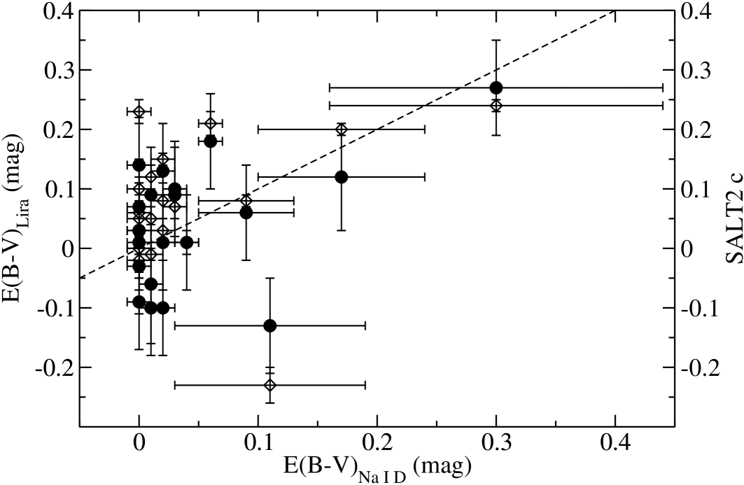
Figure 1: $E(B-V)$ as derived from the Lira relation (filled circles) or the SALT2 $c$ parameter (open diamonds) as fit from SNIFS spectrophotometry, vs. $E(B-V)$ as derived from the equivalent width of Na 1 D absorption (Poznanski et al., 2012, filled circles). The dotted line shows $E(B-V)_{\mathrm{Lira}}=E(B-V)_{\mathrm{Na~{}I~{}D}}$.

Since the Lira relation uses the same late-time data as our mass reconstruction analysis, it can serve as a separate consistency check on our data quality. If a supernova has a Lira excess inconsistent with the extinction implied by Na 1 D absorption, this could signal a problem with the late time data (e.g., residual host galaxy contamination). Figure 1 plots Lira excess against reddening derived from $EW(\mathrm{\text{Na\,\textsc{1}}~{}D)}$ and against SALT2 $c$. SNF 20070902-018 shows up as an outlier with $E(B-V)_{\mathrm{Lira}}=-0.14\pm 0.08$ mag, in rough agreement with $c=-0.23\pm 0.03$, but $E(B-V)_{\mathrm{\text{Na\,\textsc{1}}~{}D}}=0.11^{+0.11}_{-0.06}$ mag. Since $E(B-V)_{\mathrm{\text{Na\,\textsc{1}}~{}D}}$ is different from zero at less than 95% confidence, SNF 20070902-018 could simply have scattered left on the diagram, or could have Na 1 D absorption not associated with dust extinction. For the other SNe, the two reddening estimates are consistent with each other within the errors, given the substantial spread of the extinction relations. Most of our sample shows evidence for little or no host galaxy extinction. The reddening estimates also track SALT2 $c$ within the uncertainties.

3.2 Near-Infrared Corrections

Since SNIFS observes only wavelengths from 3300–9700 Å, some fraction of the bolometric flux at near-infrared wavelengths will be lost. We correct for this fraction using mean time-dependent corrections derived from near-infrared $YJHK$ photometry of normal SNe Ia from the Carnegie Supernova Project (CSP; Folatelli et al., 2010; Stritzinger et al., 2011).

We start with the 67 SNe Ia published in CSP DR2 (Stritzinger et al., 2011). To minimize the impact of dust extinction, we remove 16 SNe that have SALT2 $c>0.15$ and are therefore likely to suffer significant host reddening (including the highly extinguished SN 2006X). We also remove two superluminous SNe Ia, SN 2007if (Scalzo et al., 2010; Yuan et al., 2010) and SN 2009dc (Silverman et al., 2011; Taubenberger et al., 2011).

For the remaining 49 CSP SNe Ia, we perform Gaussian process (GP) regression to predict the $YJHK$ magnitudes between rest-frame $B$-band phases ($-14$ d, $+70$ d). The GP regression fit to all NIR observations of these CSP supernovae is then used as a template to predict the $YJHK$ magnitudes for the SNfactory sample. Before fitting, the CSP light curve in each band $j\in\{Y,J,H,K\}$ is normalized to the $i$-band flux at first maximum, $i_{\mathrm{max}}$, so that the quantity predicted by the fit is $i_{\mathrm{max}}-m_{j}$. To recover the expected NIR magnitudes for a SNfactory SN, we measure $i_{\mathrm{max}}$ and apply the measured value to the GP predictions. Normalizing the NIR correction relative to $i$-band, which suffers less extinction than $B$ or the total $UBVRI$ quasi-bolometric flux, results in a lower systematic error on the NIR correction than if we normalized it instead to the $B$-band flux or the quasi-bolometric $UBVRI$ flux. The GP regression fit in each band is shown in Figure 2; further details on the GP training, e.g. the covariance function, can be found in Appendix A.2.

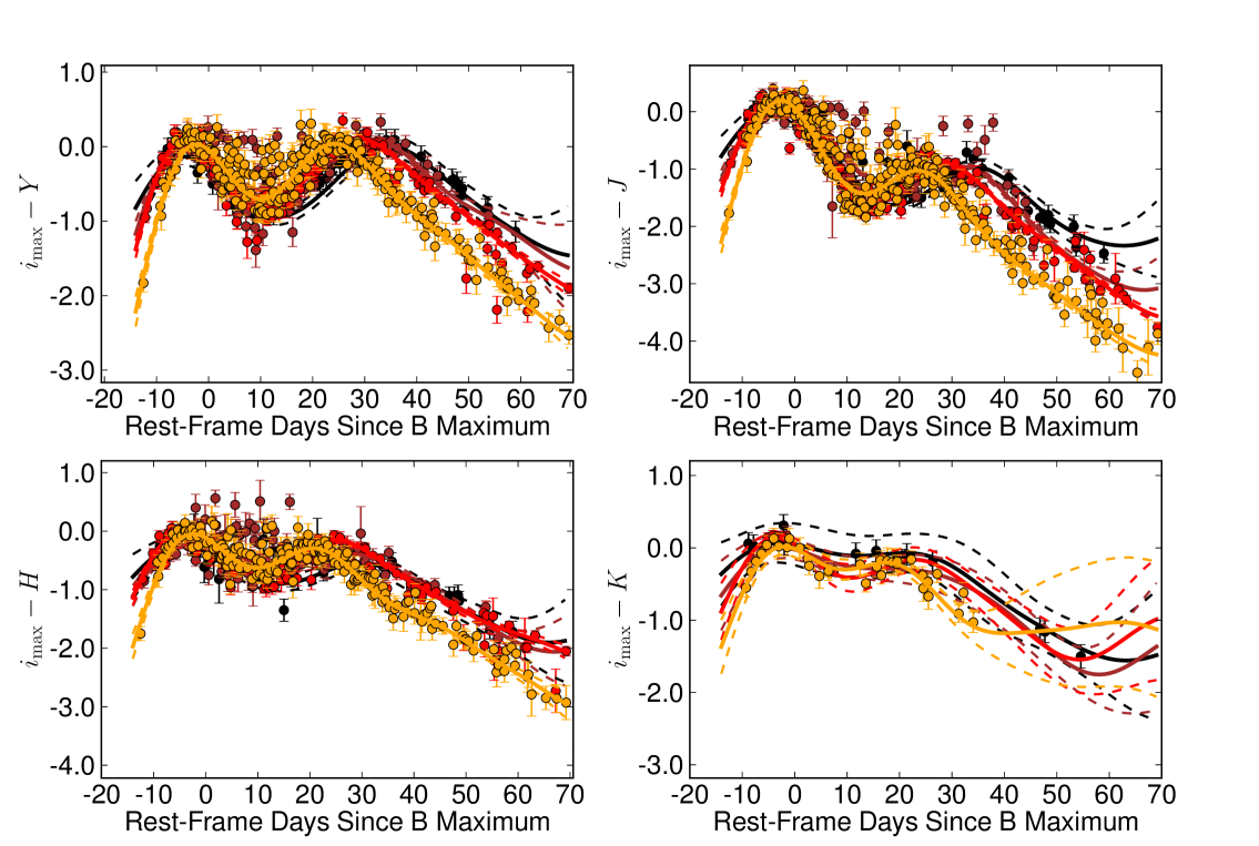
Figure 2: Gaussian process regression modeling for $YJHK$ magnitudes of normal SNe Ia from the Carnegie Supernova Project (Folatelli et al., 2010; Stritzinger et al., 2011). Bands shown: $Y$ (upper left), $J$ (upper right), $H$ (lower left), and $K$ (lower right). Sections of the GP posterior in ranges of $x_{1}$ are also shown for each band, along with the CSP data points: $-2<x_{1}<-1$ (yellow), $-1<x_{1}<0$ (red), $0<x_{1}<+1$ (brown), $+1<x_{1}<+2$ (black).

To generate a bolometric light curve from SNIFS spectrophotometry, we start with rest-frame, flux-calibrated SNIFS spectra which have been corrected for Milky Way dust extinction using the Schlegel et al. (1998) dust maps and a Cardelli et al. (1988) reddening law with $R_{V}=3.1$. We first synthesize the rest-frame $i$-band light curve of the SN and use GP regression to fit the light curve near maximum light, measuring $i_{\mathrm{max}}$. For each SNIFS spectrum, we predict $YJHK$ apparent magnitudes using the GP regression model with parameters $(x_{1},t,i_{\mathrm{max}})$ as input. We convert each predicted magnitude $m_{j}$ to a monochromatic flux density $f_{\lambda_{j}}$ at the central wavelength of CSP band $j$:

$$f_{\lambda_{j}}=10^{-0.4(m_{j}-m_{S,j})}\frac{\int S(\lambda)T_{j}(\lambda)\,d\lambda}{\int T_{j}(\lambda)\,d\lambda}$$ (1)

where $S(\lambda)$ is the SED of $\alpha$ Lyr (Bohlin & Gilliland, 2004), with magnitude $m_{S,j}$ in band $j$ with transmission $T_{j}(\lambda)$. We then interpolate linearly between these flux densities to produce a low-resolution SED, which extends the SNIFS SED at wavelengths redder than 8800 Å rest-frame. We integrate the resulting SED from 3300–23900 Å to produce a bolometric flux at each phase.

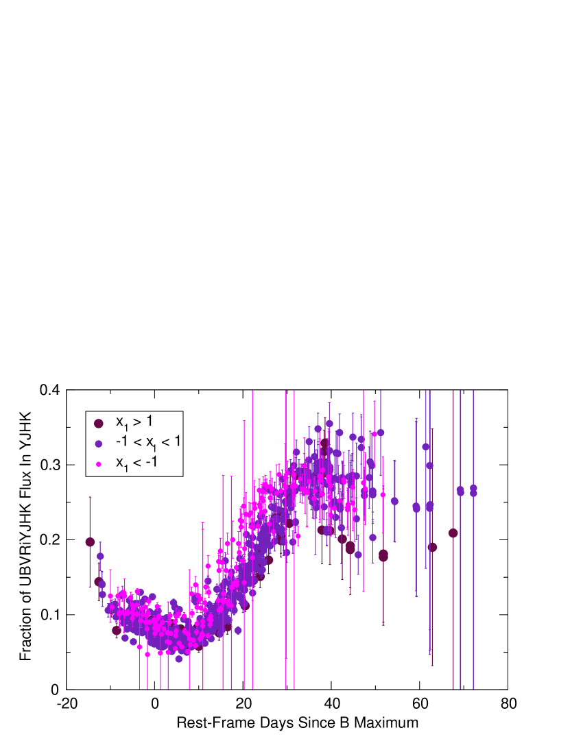
Figure 3: NIR correction for unobserved flux in the wavelength range 8800–23900 Å for the SNfactory SNe Ia, before correcting for host galaxy extinction. Three ranges in the light curve width parameter $x_{1}$ are shown here: fast-declining ($x_{1}<-1$, small magenta); average ($-1<x_{1}<1$, purple); and slow-declining ($x_{1}>1$, large maroon).

The predicted fraction of bolometric flux redward of 8800 Å as a function of rest-frame $B$-band phase for the SNfactory SNe is presented in Figure 3. While under 10% near maximum light, the fraction grows to about 30% near the NIR second maximum, and then slowly declines. The fraction is decline-rate dependent, and not negligible at late phases.

3.3 Final Bolometric Light Curves

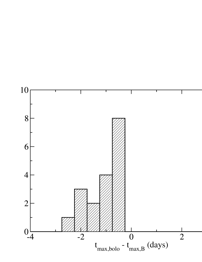
Figure 4: Difference between dates of bolometric maximum and $B$-band maximum for 19 SNe Ia in our sample.

For each SN in our sample, we generate a series of bolometric light curves corresponding to different assumptions about host galaxy reddening. Using a Cardelli extinction law with $R_{V}=3.1$ and assumed values of $E(B-V)_{\mathrm{host}}$ in 0.01 mag steps from zero to 0.40 mag, we de-redden the SNIFS spectra before performing the integration and NIR correction mentioned in §3.2. The ejected mass reconstruction (see §4) marginalizes (integrates) the posterior probability over values of the host galaxy reddening subject to a Gaussian prior given by the constraints in Table LABEL:tbl:hostred.

To ensure that all light curves in our sample have coverage at epochs appropriate for our modeling, we use a GP regression fit to the bolometric flux to extract the date of bolometric maximum light and the maximum bolometric flux. We use the fitted bolometric maximum flux to constrain the ${}^{56}\mathrm{Ni}$ mass in our reconstruction.

Figure 4 shows a histogram of the dates of bolometric maximum light, relative to the respective dates of $B$-band maximum light from the SALT2 fit, for the SNe in our sample. Four of our SNe (SNF 20061020-000, SNF 20070817-003, SNF 20080522-011, and SNF 20080620-000) have poor constraints on the date of bolometric maximum light from the GP fit, due to broad-topped light curves or too few early points with full wavelength coverage; however, their dates of $B$-band maximum light are well-constrained via SALT2, using information from multiple bands. For these SNe, we fix the date of bolometric maximum light to equal $B$-band maximum minus 1 day. (The mean of the distribution is $-1.1$ days; the median is $-0.9$ days.)

We use independent Cepheid distance estimates to determine the distance moduli when they are available (SN 2005el, SN 2008ec, SN 2011fe). For the other SNe, we derive a distance modulus for each SN from its CMB-centric host galaxy redshift assuming a $\Lambda$CDM cosmology ($\Omega_{\mathrm{M}}=0.28$, $\Omega_{\Lambda}=0.72$, $H_{0}=72$ $\mathrm{km~{}s}^{-1}$ Mpc^-1). The resulting absolute bolometric light curves are the input to our mass reconstruction in §4.

4 Modeling

For reconstruction of ${}^{56}\mathrm{Ni}$ masses and ejected masses of the SNfactory SNe Ia, we use a new implementation of the Markov chain Monte Carlo code featured in Scalzo et al. (2012), to which we refer the interested reader for a more detailed discussion of the physics involved. We summarize the overall method briefly here in §4.1, and describe our fiducial set of priors in §4.2. We test the code on a suite of contemporary SN Ia explosion models in §4.3 and discuss features of the dependence of the bolometric light curve on the physical parameters of the system in §4.4, before discussing application of the method to SNfactory observations in subsequent subsections.

4.1 The Reconstruction Method

Our reconstruction code calculates the late-time bolometric light curve in the optically thin limit of Compton scattering of gamma rays from ${}^{56}\mathrm{Co}$ decay. The code fits two parameters, a ${}^{56}\mathrm{Ni}$ mass $M_{{}^{56}\mathrm{Ni}}$ and a fiducial time $t_{0}$ at which the optical depth to Compton scattering equals unity, using Arnett’s rule (Arnett, 1982) and the analytic treatment of Jeffery (1999). The ${}^{56}\mathrm{Ni}$ mass is calculated via

$$M_{{}^{56}\mathrm{Ni}}=\frac{L_{\mathrm{bol,max}}}{\alpha\dot{S}(t_{R,\mathrm{bol}})},$$ (2)

where $L_{\mathrm{bol,max}}$ is the maximum bolometric luminosity, $t_{R,\mathrm{bol}}$ is the rise time to bolometric maximum, $\dot{S}(t)$ is the instantaneous rate of radioactive energy release from the ${}^{56}\mathrm{Ni}$ decay chain at time $t$ since explosion, and $\alpha$ is a model-dependent dimensionless number of order unity related to the diffusion time of radiation through the ejecta at early times. The transparency time $t_{0}$ at late times is calculated from

$$L_{\mathrm{bol}}(t)=\left[1-e^{-(t/t_{0})^{-2}}\right]\dot{S}_{\gamma}(t)+\dot{S}_{e^{+}}(t)$$ (3)

where we have now split $S(t)=S_{\gamma}(t)+S_{e^{+}}(t)$ into the radioactive energy release from gamma rays, some of which will escape the ejecta, and from positrons, which we treat as fully trapped at this stage of evolution of the expanding SN remnant ($t<120$ days after explosion). Note that $\alpha$ does not appear in the late-time expression; it includes reprocessing of radiation at gamma-ray and at optical wavelengths, but at late times trapping of optical radiation is much reduced and changes in gamma-ray transparency are encoded in $t_{0}$.

To first order, then, $M_{{}^{56}\mathrm{Ni}}$ controls the overall level of radioactivity and determines the overall flux scale of the light curve, while $t_{0}$ controls the rate at which the radiation escapes from the ejecta and hence the shape of the light curve. We then map these two numbers, $M_{{}^{56}\mathrm{Ni}}$ and $t_{0}$, to a total ejected mass $M_{\mathrm{ej}}$ using a Monte Carlo Markov chain (MCMC). The configuration of the model system is described by a total mass $M_{\mathrm{ej}}$, a velocity scale $v_{\mathrm{KE}}$, a central density $\rho_{c}$, a composition $(f_{\mathrm{Fe}},f_{\mathrm{{{}^{56}\mathrm{Ni}}}},f_{\mathrm{Si}},f_{\mathrm{CO}})$, and nuisance parameters $(\alpha,a_{\mathrm{Ni}},t_{R,\mathrm{bol}},E(B-V)_{\mathrm{host}})$ subject to the following prior constraints:

1. the density structure is a spherically symmetric function of velocity $\rho(v/v_{\mathrm{KE}})$;

2. the value of $v_{\mathrm{KE}}$ is set, for a given composition, via conservation of energy, by constraining the kinetic energy $E_{K}=\frac{1}{2}M_{\mathrm{ej}}v_{\mathrm{KE}}^{2}$ to be the difference between the nuclear energy $E_{N}$ (Maeda & Iwamoto, 2009) released in the explosion and the binding energy $E_{G}$ of a white dwarf of mass $M_{\mathrm{ej}}$ and central density $\rho_{c}$;

3. we use the binding energy formula of Yoon & Langer (2005), which has been used elsewhere to account for the angular momentum of rotating super-Chandrasekhar-mass white dwarfs (Howell et al., 2006; Jeffery, Branch, & Baron, 2006; Maeda & Iwamoto, 2009; Scalzo et al., 2010, 2012), and which reduces to the usual non-rotating formula for sub-Chandrasekhar-mass white dwarfs;

4. the ratio $\eta=M_{{}^{56}\mathrm{Ni}}/(M_{{}^{56}\mathrm{Ni}}+M_{\mathrm{Fe}})$ of ${}^{56}\mathrm{Ni}$ to overall iron-peak element yield is a function of $\rho_{c}$ (Krueger et al., 2010, 2012; Seitenzahl et al., 2011), with higher central densities resulting in more neutronization and a higher fraction of stable iron-peak elements;

5. mixing of ${}^{56}\mathrm{Ni}$ through the ejecta is set by a mixing parameter $a_{{}^{56}\mathrm{Ni}}$ (Kasen, 2006) which describes the scale over which mixing takes place in enclosed mass coordinates $m(v)=M_{\mathrm{ej}}^{-1}\int_{0}^{v}4\pi v^{2}\rho(v)\,dv$.

The ejected mass itself satisfies

$$M_{\mathrm{ej}}=\frac{4\pi}{\kappa_{\gamma}Q}(v_{\mathrm{KE}}t_{0})^{2},$$ (4)

where $\kappa_{\gamma}$ is the effective opacity of the ejecta to Compton scattering, and $Q$ is a form factor describing the ${}^{56}\mathrm{Ni}$-weighted Compton scattering optical depth for the given density profile and ejecta composition, similar to $q$ in (Jeffery, 1999). For a density profile with an exponential dependence on velocity, the case treated explicitly in Jeffery (1999) and in Stritzinger et al. (2006), $Q=6q$. We populate a look-up table for $Q$ as a function of the ejecta composition by numerically evaluating the necessary integrals using the VEGAS algorithm Lepage (1978), as in Scalzo et al. (2012).

We use the parallel-tempered MCMC sampler emcee (Foreman-Mackey et al., 2013), which simultaneously runs several ensembles of “walkers” with different step sizes (“temperatures”) and shares information between them. This method is appropriate for likelihood surfaces with multiple maxima, which may be the case for our problem — for example, a fast-declining light curve could in principle be described by a low-$M_{\mathrm{ej}}$ solution with a ${}^{56}\mathrm{Ni}$ distribution strongly concentrated at the centre, or by a high-$M_{\mathrm{ej}}$ solution in which the ${}^{56}\mathrm{Ni}$ lies closer to the surface. We verify that convergence has been reached by comparing runs of different lengths. In general we find a “burn-in” period of 1500 iterations, which are then discarded, suffices to remove dependence on the initial conditions. Our results are then obtained by sampling for an additional $1500\times k$ iterations, recording every $k$th iteration where $k$ is the autocorrelation time in iterations of the chain. Our final probability distributions contain about $3\times 10^{5}$ samples over all parameter configurations for each SN.

4.2 Fiducial Priors for Normal SNe Ia

Although the capabilities of the modeling code as used in this paper are the same as in Scalzo et al. (2012), we use a set of priors more appropriate for normal SNe Ia, rather than 1991T-like or super-Chandrasekhar SNe Ia. We describe these assumptions here.

Consistent with our previous work (Scalzo et al., 2010, 2012), we adopt the prior $\kappa_{\gamma}=0.025$ cm² g^-1 (Swartz et al., 1995; Jeffery, 1999), as appropriate for the case of Compton-thin ejecta. This number allows us to accurately convert from a measured column density for Compton scattering to the mass of ejecta. Most of our other priors below are targeted at making a reasonable guess about the distribution of ${}^{56}\mathrm{Ni}$ in the ejecta, which will affect our results through the form factor $Q$.

While $\alpha=1.2$ is a common choice when deriving $M_{{}^{56}\mathrm{Ni}}$ for SNe Ia (Nugent et al., 1995; Jeffery, Branch, & Baron, 2006; Howell et al., 2006, 2009), there is some uncertainty in its true value. The self-consistent, albeit simple, model of Arnett (1982) accounts for radiation trapping and has $\alpha$ very close to 1.0. The models of Höflich & Khohklov (1996) cover the range 0.8–1.6 with a mean of 1.0 and a standard deviation of 0.2. Some other analyses also fix $\alpha=1.0$ explicitly (e.g. Stritzinger et al., 2006; Mazzali et al., 2007). For compatibility with a broad range of explosion scenarios, we choose $\alpha=1.2\pm 0.2$ for our fiducial analysis. However, we also run reconstructions with fixed $\alpha=1.0$, for comparison with some of the previous literature, and to estimate how much of our final error budget results from uncertainty in the true value of $\alpha$ as derived from full simulations.

The rise time and $B$-band decline rate of normal SNe Ia are strongly correlated (Ganeshalingam et al., 2011), and since the date of bolometric maximum is strongly tied to that of $B$-band maximum, we use this information to estimate the bolometric rise time

$$t_{R,\mathrm{bol}}=t_{R,B}+(t_{\mathrm{max,bol}}-t_{\mathrm{max},B})$$ (5)

by extracting the dates $t_{\mathrm{max,bol}}$ and $t_{\mathrm{max},B}$ of maximum light of the bolometric and $B$-band light curves from the respective GP fits to those light curves. We estimate the $B$-band rise time via the relation

$$t_{R,B}=17.5-5(\Delta m_{15,B}-1.1)~{}\mathrm{days}$$ (6)

which covers the $t_{R,B}$ vs. $\Delta m_{15,B}$ locus of Ganeshalingam et al. (2011); we assign a relatively conservative error of $\pm 2$ days to this estimate. We find that bolometric maximum light precedes $B$-band maximum light by about 1 day on an average for the SNe in our sample, so our prior on $t_{R,B}$ translates to $t_{R,\mathrm{bol}}=16.5\pm 2$ days in practice for a typical SN Ia with $\Delta m_{15,B}=1.1$ (SALT2 $x_{1}=0$). For those SNe for which $B$-band maximum was fixed and not directly observed, we increase the uncertainty in the rise time to $\pm 3$ days (the spread from Figure 4).

The central density $\rho_{c}$ of the progenitor at the time of explosion influences our results through the binding energy (affecting the kinetic energy of the ejecta) and through neutronization (affecting the mass fraction of stable iron-peak elements). Seitenzahl et al. (2009) investigate the criteria for the formation of a detonation, and find that they may occur at densities as low as $3\times 10^{6}$ g cm^-3, while the lowest-mass white dwarf considered in Fink et al. (2010) had a central density of $1.4\times 10^{7}$ g cm^-3. At densities of $10^{10}$ g cm^-3 or higher, accretion-induced collapse (AIC) to a neutron star is more likely than a SN Ia explosion (Nomoto & Kondo, 1991). However, recent studies investigating the extent of neutronization in delayed detonation simulations of SN Ia explosions (Krueger et al., 2010, 2012; Seitenzahl et al., 2011), which inform our neutronization prior (see below), do not consider $\rho_{c}>5\times 10^{9}$ g cm^-3. We therefore require $7.0<\log_{10}~{}\rho_{c}<9.7$, while acknowledging that solutions with central densities outside this range could in principle exist and produce normal SNe Ia.

Since neutronization in the explosion may affect the distribution of ${}^{56}\mathrm{Ni}$ in the ejecta and hence the value of $Q$, it is important for our purposes to account for it somehow. Krueger et al. (2010) and Krueger et al. (2012) use suites of 2-D simulations to explicitly constrain the dependence of $M_{{}^{56}\mathrm{Ni}}$ and $M_{\mathrm{Fe}}$ on $\rho_{c}$. Seitenzahl et al. (2011) use a smaller suite of 3-D simulations to address the same question, with slightly larger scatter. While they disagree on how the overall iron-peak element yield varies with $\rho_{c}$, the two sets of models show similar mean behavior of $\eta(\rho_{c})$ within the scatter. We therefore adopt the Gaussian prior

$$\eta=0.95-0.05\,\rho_{c,9}\pm 0.03\,\max(1,\rho_{c,9}),$$ (7)

with $\rho_{c,9}=\rho_{c}/10^{9}$ g cm^-3, which should be consistent with both sets of simulations; as specified above, we rely on the luminosity of each SN to constrain the actual value of $M_{{}^{56}\mathrm{Ni}}$. This is slightly different than the prior used in Scalzo et al. (2012), which was informed only by the results of Krueger et al. (2010).

In Scalzo et al. (2012), we allowed our composition structure to have central concentrations of stable iron-peak elements, or central deficits of ${}^{56}\mathrm{Ni}$, for explosions of progenitors with high central density, as expected in some 1-D delayed detonation models (Khokhlov et al., 1993; Höflich & Khohklov, 1996; Blondin et al., 2013a). Recent multi-dimensional simulations of delayed detonations (Krueger et al., 2012; Seitenzahl et al., 2013), on the other hand, find no evidence for such central ${}^{56}\mathrm{Ni}$ deficits: during the deflagration phase, plumes of hot iron-peak ash rise through the ejecta rather than remaining centrally concentrated, a behavior which cannot take place in 1-D hydrodynamic models. On average, the resulting composition structure is consistent with an approximately constant ratio of ${}^{56}\mathrm{Ni}$ to stable iron-peak elements throughout the ejecta. Under this (reasonable) assumption, we find that the dependence of $Q$ on the stable iron-peak content of the ejecta is much reduced, leading to tighter constraints on the ejected mass. We therefore choose a case with no central ${}^{56}\mathrm{Ni}$ hole as our fiducial analysis. For completeness, however, we shall also explore the influence of a ${}^{56}\mathrm{Ni}$ hole. Some 3-D models, such as the violent double-degenerate mergers of Pakmor et al. (2012), show ${}^{56}\mathrm{Ni}$ holes due simply to the dynamics of the merger and not due to neutronization.

We choose $a_{\mathrm{Ni}}=0.2$, typical of the “moderate mixing” case shown in Kasen (2006). We expect that this value will reproduce the near-infrared light curves of the typical normal SN Ia, with two distinct maxima, better than the “enhanced mixing” case $a_{\mathrm{Ni}}=0.5$, which results in a strongly suppressed second maximum typical of overluminous supernovae such as the super-Chandrasekhar-mass candidates presented in Scalzo et al. (2012). While there may be some variation in the true value of $a_{\mathrm{Ni}}$ throughout the population, we use $a_{\mathrm{Ni}}=0.2$ as a representative value. In future investigations the morphology of the near-infrared light curve could in principle be used to constrain $a_{\mathrm{Ni}}$.

While it may be tempting to try to constrain $v_{\mathrm{KE}}$ by using Si 2 information near maximum light, we choose not to do so here. In Scalzo et al. (2010) and Scalzo et al. (2012), we used Si 2 absorption minimum velocities near maximum light to constrain the mass of the reverse-shock shell in a “tamped-detonation” scenario (Khokhlov et al., 1993; Höflich & Khohklov, 1996), in which the supernova ejecta interact with a dense carbon/oxygen envelope characteristic of double-degenerate mergers. However, the presence of the shell immediately implied that the photospheric velocity matched the velocity of the disturbed outer ejecta, and had no bearing on the kinetic energy scale of the bulk ejecta most relevant for the gamma-ray transparency measurement of the ejected mass. Even for SNe with smoother density structures, a variety of velocities and velocity gradients may be possible (e.g. Blondin et al., 2011, 2013a). While comparison to detailed radiation transfer models could provide constraints on $v_{\mathrm{KE}}$ from photospheric velocities, it is beyond the capacity of our current semi-analytic treatment. However, our model self-consistently predicts $v_{\mathrm{KE}}$ as a function of mass, central density, and composition. We typically obtain $v_{\mathrm{KE}}\sim 10500$ $\mathrm{km~{}s}^{-1}$, a plausible value for SNe Ia.

We limit the mass of unburned carbon and oxygen $M_{\mathrm{CO}}/M_{\mathrm{ej}}<0.05$, since carbon is rarely seen in SNe Ia except in spectra taken a week or more before maximum light (Thomas et al., 2007, 2011; Folatelli et al., 2011). This results in a constraint on $v_{\mathrm{KE}}$ and rules out models with large amounts of unburned carbon and oxygen but no intermediate-mass elements. While we use this constraint in our fiducial analysis, we will also present results without this constraint later.

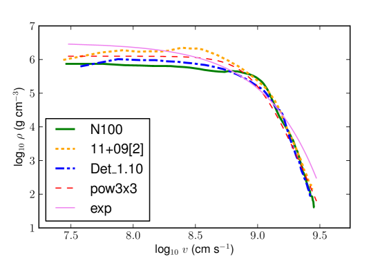
Figure 5: The “exp” and “pow3x3” density profiles, along with the angle-averaged density profiles $\rho(v)$ for three 3-D explosion models: N100 (Seitenzahl et al., 2013), 11+09 (Pakmor et al., 2012), and Det_1.10 (Ruiter et al., 2013).

Finally, the choice of density profile also affects the inferred mass through $Q$, and this choice can be informed only by hydrodynamic simulations of SN explosions. We consider two possible density profiles. An exponential density profile $\rho(v)\propto\exp(-\sqrt{12}v/v_{\mathrm{KE}})$ (“exp”) is a good description of many 1-D explosion models (Nomoto et al., 1984; Khokhlov et al., 1993; Höflich & Khohklov, 1996; Blondin et al., 2013a) and a mathematically convenient assumption in previous SN Ia work (Jeffery, 1999; Stritzinger et al., 2006; Jeffery, Branch, & Baron, 2006; Kasen, 2006). For consistency with this prior work we use an exponential density profile in our fiducial analysis. However, our framework is flexible and allows for arbitrary density profiles, so here we also consider $\rho(v)\propto[1+(v/v_{\mathrm{KE}})^{3}]^{-3}$ (“pow3x3”), which reduces to a power law $v^{-9}$ at large velocities. The “pow3x3” profile was chosen specifically to provide a structure representative of the 3-D explosion models discussed in §4.3 below. A visual comparison of the density profiles of representative explosion models with our density profiles of choice is shown in Figure 5. We could also consider highly disturbed density profiles appropriate to tamped detonations or pulsating delayed detonations (Khokhlov et al., 1993; Höflich & Khohklov, 1996), as in our previous work on candidate super-Chandrasekhar-mass SNe Ia (Scalzo et al., 2010, 2012). However, the late-time bolometric light curve is sensitive mainly to the overall column density presented to outbound ${}^{56}\mathrm{Co}$ gamma rays (i.e., on $Q$). A density enhancement due to a shock in the outer layers will not influence $Q$ as long as it does not extend into the ${}^{56}\mathrm{Ni}$-rich inner ejecta.

The results of the mass reconstruction for our fiducial analysis are shown in Table LABEL:tbl:massrecon. Since the probability distributions of the tabulated quantities are significantly non-Gaussian, the (asymmetric) error bars we quote bound the 68% confidence region. We also tabulate the probability $P(>M_{\mathrm{Ch}})$ that the SN’s mass exceeds 1.4 $M_{\odot}$, very high or low values of which indicate significant deviation from a Chandrasekhar-mass explosion.

Table 3: Mass reconstruction of SNfactory bolometric light curves

SN Name	${M_{\mathrm{ej}}/M_{\odot}}^{\mathrm{a}}$	${M_{{}^{56}\mathrm{Ni}}/M_{\odot}}^{\mathrm{b}}$	${t_{0}}^{\mathrm{c}}$ (days)	${P_{\mathrm{SCh}}}^{\mathrm{d}}$	${P_{\mathrm{fit}}}^{\mathrm{e}}$
SNfactory-Discovered Supernovae
SNF 20060907-000	$1.01^{+0.09}_{-0.07}$	$0.56\pm 0.12$	$33.8\pm 4.1$	$0.001$	$0.797$
SNF 20061020-000	$0.99^{+0.11}_{-0.09}$	$0.34\pm 0.09$	$37.8\pm 4.4$	$0.002$	$0.355$
SNF 20070506-006†	$1.53^{+0.17}_{-0.11}$	$0.71\pm 0.14$	$47.4\pm 5.8$	$0.885$	$0.788$
SNF 20070701-005	$1.31^{+0.11}_{-0.10}$	$0.83\pm 0.17$	$38.3\pm 4.1$	$0.224$	$0.438$
SNF 20070810-004	$1.35^{+0.15}_{-0.17}$	$0.40\pm 0.08$	$47.3\pm 6.3$	$0.392$	$0.730$
SNF 20070817-003	$1.04^{+0.12}_{-0.10}$	$0.33\pm 0.09$	$39.6\pm 4.8$	$0.011$	$0.717$
SNF 20070902-018	$1.18^{+0.15}_{-0.13}$	$0.36\pm 0.08$	$43.1\pm 5.2$	$0.081$	$0.364$
SNF 20080522-011	$1.40^{+0.12}_{-0.12}$	$0.61\pm 0.15$	$45.0\pm 5.7$	$0.518$	$0.355$
SNF 20080620-000	$1.14^{+0.16}_{-0.12}$	$0.32\pm 0.07$	$42.7\pm 5.2$	$0.070$	$0.775$
SNF 20080717-000	$1.46^{+0.12}_{-0.09}$	$0.80\pm 0.20$	$43.3\pm 4.9$	$0.735$	$0.204$
SNF 20080803-000	$1.34^{+0.13}_{-0.13}$	$0.61\pm 0.15$	$42.5\pm 5.4$	$0.333$	$0.711$
SNF 20080913-031	$1.10^{+0.12}_{-0.10}$	$0.43\pm 0.09$	$39.2\pm 4.7$	$0.015$	$0.782$
SNF 20080918-004	$0.92^{+0.08}_{-0.06}$	$0.30\pm 0.05$	$36.4\pm 3.0$	$0.000$	$0.733$
Externally Discovered Supernovae Observed by SNfactory
SN 2005el	$0.90^{+0.06}_{-0.05}$	$0.52\pm 0.12$	$31.4\pm 3.0$	$0.000$	$0.570$
SN 2007cq	$1.17^{+0.12}_{-0.10}$	$0.53\pm 0.12$	$39.4\pm 4.9$	$0.046$	$0.738$
SN 2008ec	$1.02^{+0.10}_{-0.09}$	$0.34\pm 0.08$	$38.5\pm 4.0$	$0.002$	$0.506$
SN 2011fe	$1.19^{+0.12}_{-0.11}$	$0.42\pm 0.08$	$42.4\pm 4.5$	$0.057$	$0.585$
PTF09dlc	$1.24^{+0.14}_{-0.11}$	$0.48\pm 0.10$	$42.4\pm 5.3$	$0.129$	$0.772$
PTF09dnl	$1.33^{+0.13}_{-0.13}$	$0.48\pm 0.10$	$45.2\pm 5.3$	$0.324$	$0.509$

4.3 Reconstruction of Simulated Light Curves

As a test of the code, we have run our reconstruction code on a set of simulated bolometric light curves of numerical explosion models generated with the Monte Carlo radiation transfer code ARTIS (Kromer & Sim, 2009). The models span a range of masses from 1.06 $M_{\odot}$ to 1.95 $M_{\odot}$ and different explosion mechanisms, and provide synthetic observables from well before bolometric maximum to about 75 days after bolometric maximum. We assign an error of 0.03 mag to each point, although the actual light curves have much lower statistical noise; this represents approximately what our method could achieve in the limit of very high signal-to-noise. The models were reconstructed in a blind analysis, using the same input assumptions as our fiducial analysis (“Run A” in §4.7) on the SNfactory sample, with the model identities and true ejected masses and ${}^{56}\mathrm{Ni}$ masses unknown until the reconstruction had been performed.

The results of the reconstruction are shown in Table LABEL:tbl:massrecon-mpa, along with the unblinded model identities and references. We remind the reader that our Monte Carlo sampler does not search for a single set of best-fitting parameters for a given light curve, but samples the entire probability distribution of allowed parameter values. The columns in the table represent projections of this probability distribution onto the variables of interest, marginalizing (i.e. integrating) over all other variables. Since the probability distributions for the reconstructed quantities are in general asymmetric with non-Gaussian tails, we quote the median value as the central value estimate with the 68% confidence intervals expressed as asymmetric error bars, and also show the total integrated probability of the reconstructed parameters above $M=M_{\mathrm{Ch}}=1.4~{}M_{\odot}$.

Table 4: Mass reconstruction of simulated bolometric light curves

	True Parameters		Reconstructed Parameters
SN Name	${M_{\mathrm{ej}}/M_{\odot}}^{\mathrm{a}}$	${M_{{}^{56}\mathrm{Ni}}/M_{\odot}}^{\mathrm{b}}$	${M_{\mathrm{ej}}/M_{\odot}}^{\mathrm{a}}$	${M_{{}^{56}\mathrm{Ni}}/M_{\odot}}^{\mathrm{b}}$	${t_{0}}^{\mathrm{c}}$ (days)	${P_{\mathrm{SCh}}}^{\mathrm{d}}$	${P_{\mathrm{fit}}}^{\mathrm{e}}$
Using Full Late-Time Light Curve
Model 3f	1.07	0.60	$1.01^{+0.09}_{-0.08}$	$0.34\pm 0.05$	$38.3\pm 3.5$	$0.002$	$0.577$
Det_1.10g	1.10	0.62	$1.22^{+0.12}_{-0.11}$	$0.38\pm 0.06$	$44.1\pm 4.3$	$0.089$	$0.579$
N5h	1.40	0.97	$1.35^{+0.11}_{-0.11}$	$0.60\pm 0.10$	$43.5\pm 4.6$	$0.331$	$0.712$
N100h	1.40	0.60	$1.27^{+0.14}_{-0.12}$	$0.40\pm 0.07$	$45.0\pm 5.0$	$0.197$	$0.917$
N1600h	1.40	0.32	$1.46^{+0.18}_{-0.11}$	$0.21\pm 0.02$	$55.9\pm 4.3$	$0.713$	$0.689$
11+09[1]i	1.95	0.62	$1.87^{+0.38}_{-0.18}$	$0.42\pm 0.05$	$64.7\pm 5.8$	$1.000$	$0.890$
11+09[2]i	1.95	0.62	$1.66^{+0.15}_{-0.10}$	$0.91\pm 0.14$	$47.6\pm 4.7$	$1.000$	$0.662$
11+09[3]i	1.95	0.62	$1.59^{+0.22}_{-0.13}$	$0.37\pm 0.04$	$57.1\pm 4.6$	$0.957$	$0.792$
Using Only Data at +40 Days
Model 3f	1.07	0.60	$1.08^{+0.11}_{-0.10}$	$0.34\pm 0.05$	$39.2\pm 4.1$	$0.005$	$0.669$
Det_1.10g	1.10	0.62	$1.17^{+0.12}_{-0.11}$	$0.41\pm 0.07$	$40.8\pm 4.6$	$0.047$	$0.810$
N5h	1.40	0.97	$1.33^{+0.11}_{-0.11}$	$0.63\pm 0.11$	$40.8\pm 4.7$	$0.300$	$0.786$
N100h	1.40	0.60	$1.28^{+0.14}_{-0.13}$	$0.41\pm 0.07$	$43.7\pm 5.2$	$0.218$	$0.764$
N1600h	1.40	0.32	$1.41^{+0.16}_{-0.17}$	$0.23\pm 0.03$	$51.9\pm 5.6$	$0.521$	$0.679$
11+09[1]i	1.95	0.62	$2.00^{+0.57}_{-0.30}$	$0.42\pm 0.07$	$65.9\pm 10.3$	$0.999$	$0.752$
11+09[2]i	1.95	0.62	$1.66^{+0.15}_{-0.10}$	$0.97\pm 0.15$	$44.9\pm 4.9$	$1.000$	$0.637$
11+09[3]i	1.95	0.62	$1.76^{+0.46}_{-0.24}$	$0.34\pm 0.05$	$60.8\pm 8.9$	$0.972$	$0.740$

The reconstructed masses agree surprisingly well with the model masses, given that the input assumptions were not tuned to match the explosion models. In general the reduced chi-squares are modest, showing that the Jeffery (1999) functional form can provide a good description of the simulated light curves within the time range in which it applies. The true ejected mass lies within the formal 68% confidence interval on $M_{\mathrm{ej}}$ for five of the eight cases, and within the 95% confidence interval for all eight cases. Just as importantly for our purposes, except for the sub-Chandrasekhar model Det_1.10, the code correctly distinguishes the non-Chandrasekhar-mass models at high significance ($>95\%$ CL) from the Chandrasekhar-mass models.

Three of the light curves represent different lines of sight for the same violent merger model 11+09, with $M_{\mathrm{ej}}=1.95~{}M_{\odot}$, $M_{{}^{56}\mathrm{Ni}}=0.62~{}M_{\odot}$ (Pakmor et al., 2012): the angle-averaged light curve and the brightest and faintest viewing angles. Our method gives a very accurate result for the angle-averaged light curve, but slightly underestimates the ejected mass in both asymmetric views. However, in each case it still correctly identifies the event as super-Chandrasekhar at high ($>95\%$ CL) significance. The angle-averaged ${}^{56}\mathrm{Ni}$ fraction has a hole in the centre (see figure 2 of Pakmor et al., 2012), though it originates from an interaction with the secondary star rather than neutronization. When this is accounted for in our priors, the reconstructed masses of versions 1, 2, and 3 become $2.31^{+0.26}_{-0.37}~{}M_{\odot}$, $1.83^{+0.37}_{-0.23}~{}M_{\odot}$, and $1.94^{+0.33}_{-0.30}~{}M_{\odot}$, respectively, with the true value within the 68% CL interval for each reconstruction.

The derived ${}^{56}\mathrm{Ni}$ masses are less secure. They are quite wrong for the asymmetric views of 11+09, as one might expect since Arnett’s rule assumes spherical ejecta. This suggests that some, though not necessarily all, events which appear to have too much ${}^{56}\mathrm{Ni}$ for their reconstructed mass may in fact be bright views of an asymmetric explosion. In such a scenario we would expect more variation in the derived $M_{{}^{56}\mathrm{Ni}}$/$M_{\mathrm{ej}}$ ratio for low-${}^{56}\mathrm{Ni}$ events. For models with less pronounced asymmetries, such as the N5, N100 and N1600 delayed detonations, the reconstructed value of $M_{{}^{56}\mathrm{Ni}}$ is in general about 50% lower than the true value. This is due to a combination of factors: the actual value of $\alpha$ is closer to 1.0 in the simulations than the central value of 1.2 we assume for our prior, and some of the models (for example, N100) have more high-velocity ${}^{56}\mathrm{Ni}$ than we assume, affecting the interpretation of the late-time light curves.

Since the reconstructed mass distributions are non-Gaussian, the pull distribution $(M_{\mathrm{ej}}-M_{\mathrm{WD,true}})/\sigma_{M_{\mathrm{WD}}}$ will not have its usual interpretation, but may still be useful as an indication of how far wrong our reconstructions are, and in which direction. Using the appropriate one-sided 68% uncertainty for each object, we find that the pull distribution has mean $-0.52$ and standard deviation 0.95; an unbiased sample drawn from a Gaussian should have mean within $[-0.35,0.35]$ (1$\sigma$) and width near 1. Thus, within this small but fairly diverse selection of explosion models, our baseline assumptions seem to incur only a small bias, if any. The uncertainties scale with mass, with sub-Chandrasekhar-mass reconstructions being the most secure in absolute terms.

Table LABEL:tbl:massrecon-mpa also includes results where we use only the first light curve point more than 40 days after bolometric maximum, since many of our SNe will have only this point at late times. This makes the minimum value of $\chi^{2}/\nu$ meaningless as a hypothesis testing measure, since the fit will not be overconstrained, but the Monte Carlo sampler will still be able to use the likelihood to reject models which do not fit the data. The results are largely unchanged; the pull distribution is not dramatically different (mean $-0.35$, standard deviation $0.75$), and the true ejected masses still lie within the 95% CL interval for all eight models. The code also still accurately distinguishes between sub-Chandrasekhar, Chandrasekhar-mass and super-Chandrasekhar explosions. While the reconstruction may therefore be slightly less accurate and/or precise for SNe Ia with fewer or less accurate late-time photometry points, the broad trends of the mass distribution are still preserved.

In summary, while the code does not perform perfectly on every input model, it does at least seem to provide reasonable estimates of the uncertainties: 62.5% of the models lie within the 68% confidence region. The results give us some confidence that the method is relatively robust to systematics, and that it should accurately recover the ejected mass of most input SNe Ia from a range of contemporary progenitor scenarios. We refrain from fine-tuning our priors to match this suite of models, since it is a small set using one radiation transfer code and any tuning attempts may be prone to overfitting, but we explore some different plausible priors in order to bound the associated systematics.

4.4 Comparing Model Light Curve with Data

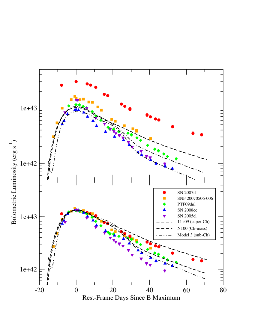
Figure 6: Observed bolometric light curves of representative SNfactory SNe Ia (coloured symbols with error bars), alongside synthetic observables for explosion models (black curves). Top: original light curves; bottom: light curves normalized to a peak luminosity of $1.2\times 10^{43}$ erg s^-1.

To build confidence that our method is capturing useful distinctions between SNe of different masses, we show a direct comparison between SNfactory light curves and three representative explosion models in Figure 6. The light curves as actually observed are shown on the top, while on the bottom, they are normalized to the same peak luminosity to emphasize differences in shape.

The models, all with $M_{{}^{56}\mathrm{Ni}}=0.6$ $M_{\odot}$ but with differing ejected masses, are shown as black curves. The overall trend with light curve shape is clear: the (angle-averaged) light curve of the super-Chandrasekhar-mass violent merger 11+09 is the brightest at $+40$ days, followed by those of the Chandrasekhar-mass delayed detonation N100 and the sub-Chandrasekhar-mass double detonation Model 3. The less massive models show inflections corresponding to the NIR second maximum, but all have settled down into an optically thin, quasi-exponential decline by $+40$ days (Jeffery, 1999).

The real SNfactory SNe span a broader range of ${}^{56}\mathrm{Ni}$ mass and so show a spread of absolute magnitudes, but the light curve shapes are usually quite similar to the models for corresponding reconstructed masses. SN 2007if, with $M_{\mathrm{ej}}=2.30^{+0.27}_{-0.24}$ $M_{\odot}$ (Scalzo et al., 2012), has a broad, uninflected light curve with a decay rate similar to the 1.95-$M_{\odot}$ model 11+09; it is three times more luminous overall, and seems to decline slightly more rapidly than 11+09. The difference in decline rate may be a sign that more radiation is being trapped or produced near maximum light, or that more radiation is escaping at late times from ${}^{56}\mathrm{Co}$ in higher-velocity ejecta. PTF09dnl ($M_{\mathrm{ej}}=1.33^{+0.13}_{-0.13}~{}M_{\odot}$) closely resembles the Chandrasekhar-mass model N100, and SN 2008ec ($M_{\mathrm{ej}}=1.02^{+0.10}_{-0.09}~{}M_{\odot}$) closely resembles the sub-Chandrasekhar-mass Model 3.

SN 2005el presents an interesting outlier case which we shall discuss in more detail in the following section. It has a late-time light curve similar to the sub-Chandrasekhar-mass models, but is as bright near maximum light as the Chandrasekhar-mass models; this implies a very high ${}^{56}\mathrm{Ni}$ content which should result in a peculiar spectrum, but in fact it appears spectroscopically normal.

4.5 Trends with Decline Rate

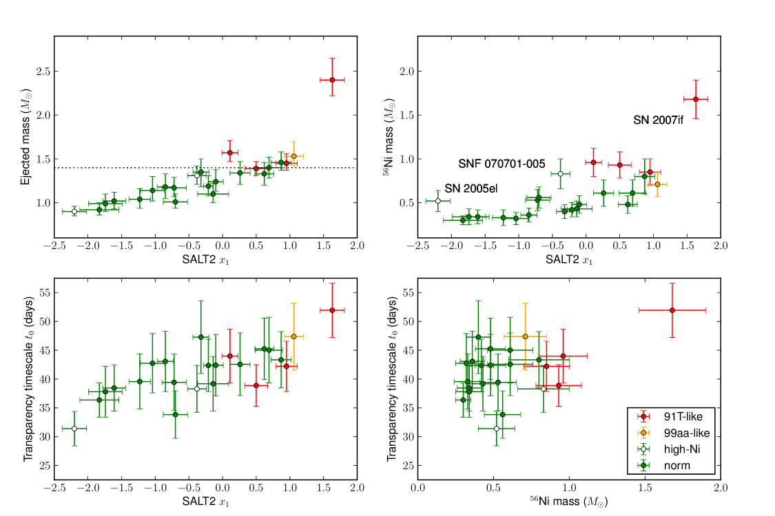
Figure 7: Correlations between reconstructed quantities and light curve parameters. Different colours show different spectroscopic subtypes: red = 1991T-like/super-Chandra (Scalzo et al., 2010, 2012), orange = 1999aa-like, green = core normal. Spectroscopically normal SNe Ia which show up as outliers in the $M_{\mathrm{ej}}$-$t0$ plane are shown as open circles. The horizontal dotted line marks the Chandrasekhar mass $M=1.4~{}M_{\odot}$.

A correlation between light curve decline rate and ejected mass is expected for SNe Ia (e.g. Arnett, 1982), and indeed for radioactively powered SNe in general, since the diffusion time for optical photons should increase with mass. The scaling relations of Arnett (1982) are frequently used by observers to obtain rough estimates of the ejected masses of supernovae (e.g. Sullivan et al., 2011; Drout et al., 2011; Cano et al., 2013). However, the degeneracy between the ejected mass and other factors affecting the diffusion time, including the ejecta velocity and opacity to optical-wavelength photons, severely limits the accuracy of mass predictions from near-maximum-light data. Opacities in particular depend on the temperature and composition and may therefore vary with time (Khokhlov et al., 1993). In contrast, our method, which relies on the well-understood, nearly-gray opacity of Compton scattering in the optically-thin limit (Swartz et al., 1995; Jeffery, 1999), has the potential to break the degeneracies and shed light on the relationship between mass and near-maximum-light decline rate.

Figure 7 shows the dependence of the underlying parameters $M_{{}^{56}\mathrm{Ni}}$ and $t_{0}$, and of the inferred mass $M_{\mathrm{ej}}$, on the light curve decline rate parameter $x_{1}$ for the SNfactory sample. We have colour-coded the points by spectroscopic subtype, showing 1991T-like and 1999aa-like SNe for comparison with the general population of normal SNe Ia.

Most striking is the strength of the correlation between $M_{\mathrm{ej}}$ and $x_{1}$, with very small dispersion. A measurement of the light curve shape is enough to determine the mass almost as accurately as the full fit. A similar positive correlation is seen, as expected, in $M_{{}^{56}\mathrm{Ni}}$ vs. $x_{1}$, though with more variation. Excluding two outliers which we shall discuss below, the least-square best-fitting linear trends to the data for normal SNe Ia, taking both errors in $M_{\mathrm{ej}}$ and $x_{1}$ into account, are

$$M_{\mathrm{ej}}/M_{\odot} = (1.253\pm 0.022)+(0.172\pm 0.021)\,x_{1}$$ (8)

$$M_{{}^{56}\mathrm{Ni}}/M_{\odot} = (0.478\pm 0.023)+(0.100\pm 0.020)\,x_{1}$$ (9)

with Pearson’s $r=0.900$ ($p<10^{-5}$) for $M_{\mathrm{ej}}$ vs. $x_{1}$. Although the true underlying trend may not in fact be linear, the reduced chi-squares for both fits are small: $\chi^{2}/\nu=5.9/14=0.41$ for a linear fit to $M_{\mathrm{ej}}$ vs. $x_{1}$, and $6.6/14=0.47$ for $M_{{}^{56}\mathrm{Ni}}$ vs. $x_{1}$. This suggests that some of the model-dependent parameters over which we marginalize (such as $\alpha$) may be strongly correlated with each other for a given SN, and/or may have similar values for different SNe in our sample with similar $x_{1}$, although the true values of these parameters are not accurately known. SNF 20070506-006, the only 1999aa-like SN Ia in the SNfactory sample with sufficiently high data quality at late times to be considered here, reconstructs with mass $M_{\mathrm{ej}}=1.53^{+0.17}_{-0.11}~{}M_{\odot}$, on the high end of our mass range for spectroscopically normal SNe Ia but not definitely super-Chandrasekhar-mass. Seven SNe in our fiducial analysis reconstruct as sub-Chandrasekhar at greater than 95% confidence, of which five have $x_{1}<-1$.

We re-emphasize that the $M_{\mathrm{ej}}$-$x_{1}$ correlation is not a spurious trend arising solely from any explicit dependence on $x_{1}$ in our analysis chain. The trend changes negligibly when the Ganeshalingam et al. (2011) rise-time prior is replaced by a simple Gaussian prior $t_{R,\mathrm{bol}}=17\pm 2$ days, or when the $x_{1}$-dependent NIR correction is replaced by a mean correction. The dependence must therefore already be imprinted on the shape of the post-maximum optical light curves, as shown in Figure 6.

The transparency time $t_{0}$ also has a strong correlation with $x_{1}$, and since $t_{0}$ is derived directly from the data, this correlation is harder to explain as an artifact of our fitting procedure. Stritzinger et al. (2006) noted a similar correlation using a much simpler set of priors. We have also verified that we get the same results for two very well-sampled light curves with different reconstructed masses, SN 2007if (super-Chandra) and SN 2011fe (Chandrasekhar-mass), by fitting subsamples of the late-time light curve data, first using a single point near $B$-band phase $+40$ days and then again using only points later than $+60$ days. The median reconstructed mass changes by less than 0.03 $M_{\odot}$ in each case.

Starting from the fast-declining end, $t_{0}$ increases sharply with $x_{1}$ at first; the slope decreases for $x_{1}>-1$. Such a break may also appear in the $M_{\mathrm{ej}}$-$x_{1}$ plane, although if it does, it is less dramatic. Finally, the plot of $M_{{}^{56}\mathrm{Ni}}$ vs. $t_{0}$, the closest we can come to the raw data, shows no particularly strong trend, although this is not in itself surprising since the two parameters are functionally independent in the Arnett (1982) formalism. SNe with 1991T-like and 1999aa-like maximum-light spectra cluster at the slowly-declining, slowly-diffusing, high-$M_{{}^{56}\mathrm{Ni}}$, high-$M_{\mathrm{ej}}$ end of each plot; all of the spectroscopically peculiar SNe Ia studied in Scalzo et al. (2012) have $M_{{}^{56}\mathrm{Ni}}>0.8~{}M_{\odot}$.

Two of our SNe, SN 2005el and SNF 20070701-005, are outliers in the $M_{{}^{56}\mathrm{Ni}}$-$x_{1}$ plane. The reconstructions for these two SNe show very high $M_{{}^{56}\mathrm{Ni}}$ ($\sim 0.7\,M_{\mathrm{ej}}$) typical of 1991T-like or super-Chandra SNe, yet they appear spectroscopically normal. We discuss these below.

SNF 20070701-005 originally reconstructs with $M_{\mathrm{ej}}=1.31^{+0.11}_{-0.10}$ $M_{\odot}$ and $M_{{}^{56}\mathrm{Ni}}=0.83\pm 0.17$ $M_{\odot}$. The derived host galaxy reddening from $EW(\mathrm{\text{Na\,\textsc{1}}~{}D)}$ and from the Lira relation are nearly identical, making the intrinsic $B-V$ colour of the SN at $B$-band maximum light near zero. Our measured absolute magnitude for this SN is also comparable to the 1999aa-like SNF 20070506-006, mentioned above. The behavior of this SN near maximum light is less well-constrained than for our other SNe, and the uncertainty on the reddening is larger, leading to a larger uncertainty in the ${}^{56}\mathrm{Ni}$ mass. This SN may simply have scattered up on the diagram, or may show mild departures from the particular assumptions of our method. We expect our ejected mass estimate to be relatively robust to large uncertainties in the ${}^{56}\mathrm{Ni}$ mass (see §4.7); note also SNF 20080717-000, which has the most uncertain ${}^{56}\mathrm{Ni}$ mass estimate in our sample, but for which the ejected mass is relatively well-constrained. The ejected mass of SNF 20070701-005 is consistent with the Chandrasekhar mass and its behavior is not unusual in any other respect.

SN 2005el presents a more interesting case. It has one of the best-sampled SNIFS spectrophotometric time series, with several late-time points and reproducible bolometric light curve precision at the 0.02 mag level. It is the fastest-declining SN in our sample ($x_{1}=-2.20$), with a robust NIR second maximum, $EW(\mathrm{\text{Na\,\textsc{1}}~{}D)}$ and Lira excesses consistent with zero reddening, and a peak absolute bolometric luminosity of $1.3\times 10^{43}$ erg s^-1, consistent with $\sim 0.6~{}M_{\odot}$ of ${}^{56}\mathrm{Ni}$ under Arnett’s rule. Others have confirmed these observed properties (Phillips et al., 2007; Hicken et al., 2009). SN 2005el may have physical properties which are not well-represented by our model. The least exotic possibility is that our priors are wrong, and that this SN is best described with a higher value of $\alpha$ and/or a shorter rise time, so that less ${}^{56}\mathrm{Ni}$ is required to describe the peak bolometric luminosity we measure. The value of $\alpha$ required to make SN 2005el resemble SNF 20080918-004, which has the most similar mass, must be very large, at least 1.6. SN 2005el could also have an unusual density structure, or could be asymmetric. In any case, if our mass reconstruction is correct, it is more likely that SN 2005el actually has less ${}^{56}\mathrm{Ni}$ than our fiducial analysis suggests.

4.6 Trends with Color and $EW(\mathrm{Na~{}I~{}D})$

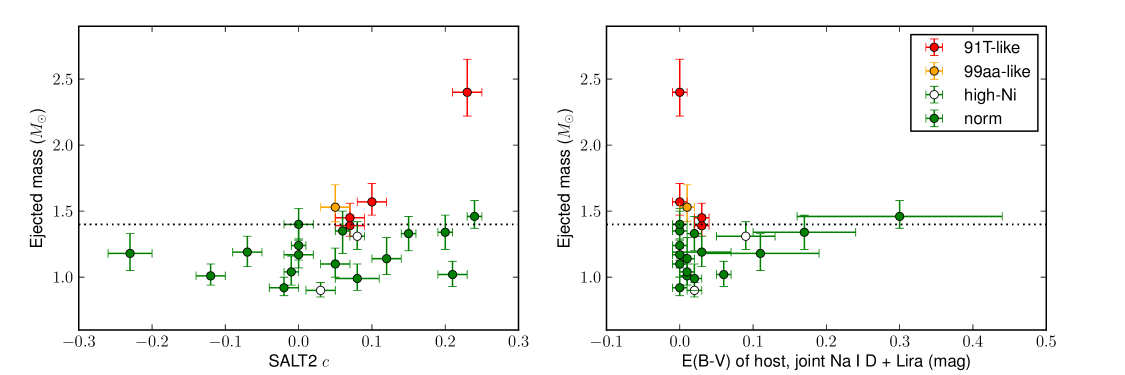
Figure 8: Correlations between reconstructed quantities and extinction measures. Colors represent different spectroscopic subtypes, as in Figure 7. The horizontal dotted line marks the Chandrasekhar mass $M=1.4~{}M_{\odot}$.

We are fortunate that most of the SNe in our sample show little or no evidence for host galaxy reddening. It is nevertheless worth checking to see whether a trend with SALT2 $c$ or $EW(\mathrm{\text{Na\,\textsc{1}}~{}D)}$ is apparent in the data.

Figure 8 shows the variation of $M_{{}^{56}\mathrm{Ni}}$ and $M_{\mathrm{ej}}$ with SALT2 $c$ and with $EW(\mathrm{\text{Na\,\textsc{1}}~{}D)}$. No obvious correlations appear. Most of the SNe lie down at low $EW(\mathrm{\text{Na\,\textsc{1}}~{}D)}$, where a wide range of $M_{\mathrm{ej}}$ is seen. Only three points have $E(B-V)_{\mathrm{host}}>0.06$ mag, and these also have considerable uncertainty in the reddening. SNe with large reddening corrections have uncertain $M_{{}^{56}\mathrm{Ni}}$ and may plausibly be biased towards higher $M_{\mathrm{ej}}$. However, our main conclusions — the existence of sub-Chandrasekhar-mass SNe Ia, and of a correlation between ejected mass and light curve width — are not being driven by these SNe.

4.7 Variation in Reconstruction Assumptions

Table 5: Variations in priors for different reconstruction runs

Run	$\rho(v)$a	$Q$b	$\alpha$	$M_{\mathrm{CO}}/M_{\mathrm{ej}}$
A	exp	std	$1.2\pm 0.2$	$0.00\pm 0.05$
B	pow3x3	std	$1.2\pm 0.2$	$0.00\pm 0.05$
C	exp	hole	$1.2\pm 0.2$	$0.00\pm 0.05$
D	pow3x3	hole	$1.2\pm 0.2$	$0.00\pm 0.05$
E	exp	std	$1.0$	$0.00\pm 0.05$
F	pow3x3	std	$1.0$	$0.00\pm 0.05$
G	exp	std	$1.2\pm 0.2$	$<1$
H	pow3x3	std	$1.2\pm 0.2$	$<1$
Sc	exp	$2.0\pm 0.6$	$1.0$	—

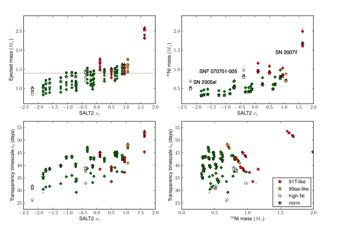
Figure 9: Influence of perturbations to input assumptions on reconstructed quantities and their correlations with light curve parameters. Colors represent different spectroscopic subtypes, as in Figure 7. Error bars have been suppressed to allow the mean values to be seen more clearly. The horizontal dotted line marks the Chandrasekhar mass $M=1.4~{}M_{\odot}$. Run A: circles; run B: squares; run C: inverted triangles; run D: triangles; run E: diamonds; run F: crosses; run G: hexagons; run H: stars.

Although the priors for our fiducial analysis are well-motivated, they are not unique, and performing many reconstructions with different input assumptions can help quantify our sensitivity to these assumptions. Some systematic effects, such as variations in $\alpha$, can be readily parametrized and incorporated into our MCMC sampler, while others (such as the radial dependence of the ${}^{56}\mathrm{Ni}$ distribution) involve the choice of a free function and/or lengthy calculations which are most effective when decoupled from the MCMC. We discuss such systematics in this section.

Table 6: Ejected masses in different reconstruction runs

SN Name	Run A	Run B	Run C	Run D	Run E	Run F	Run G	Run H	Run S
SNfactory-Discovered Supernovae
SNF 20060907-000	$1.01^{+0.09}_{-0.07}$	$1.16^{+0.15}_{-0.11}$	$1.02^{+0.10}_{-0.08}$	$1.18^{+0.17}_{-0.12}$	$0.94^{+0.05}_{-0.05}$	$1.04^{+0.07}_{-0.06}$	$0.97^{+0.09}_{-0.07}$	$1.10^{+0.14}_{-0.11}$	$0.99^{+0.49}_{-0.23}$
SNF 20061020-000	$0.99^{+0.11}_{-0.09}$	$1.21^{+0.18}_{-0.15}$	$1.00^{+0.11}_{-0.09}$	$1.21^{+0.18}_{-0.15}$	$0.87^{+0.03}_{-0.03}$	$1.01^{+0.06}_{-0.05}$	$0.96^{+0.11}_{-0.08}$	$1.12^{+0.19}_{-0.15}$	$0.90^{+0.51}_{-0.26}$
SNF 20070506-006†	$1.53^{+0.17}_{-0.11}$	$1.75^{+0.32}_{-0.18}$	$1.57^{+0.19}_{-0.13}$	$1.78^{+0.30}_{-0.18}$	$1.43^{+0.08}_{-0.06}$	$1.58^{+0.13}_{-0.09}$	$1.46^{+0.16}_{-0.12}$	$1.62^{+0.28}_{-0.17}$	$1.39^{+0.59}_{-0.34}$
SNF 20070701-005	$1.31^{+0.11}_{-0.10}$	$1.46^{+0.13}_{-0.10}$	$1.38^{+0.14}_{-0.13}$	$1.48^{+0.15}_{-0.11}$	$1.19^{+0.06}_{-0.05}$	$1.33^{+0.08}_{-0.07}$	$1.27^{+0.12}_{-0.10}$	$1.42^{+0.12}_{-0.12}$	$1.44^{+0.50}_{-0.29}$
SNF 20070810-004	$1.35^{+0.15}_{-0.17}$	$1.53^{+0.25}_{-0.14}$	$1.39^{+0.14}_{-0.18}$	$1.54^{+0.25}_{-0.14}$	$1.14^{+0.07}_{-0.06}$	$1.36^{+0.11}_{-0.09}$	$1.24^{+0.20}_{-0.17}$	$1.45^{+0.22}_{-0.19}$	$1.25^{+0.62}_{-0.39}$
SNF 20070817-003	$1.04^{+0.12}_{-0.10}$	$1.28^{+0.18}_{-0.17}$	$1.04^{+0.13}_{-0.10}$	$1.29^{+0.18}_{-0.17}$	$0.90^{+0.04}_{-0.03}$	$1.06^{+0.07}_{-0.06}$	$0.99^{+0.12}_{-0.10}$	$1.18^{+0.21}_{-0.17}$	$0.97^{+0.55}_{-0.29}$
SNF 20070902-018	$1.18^{+0.15}_{-0.13}$	$1.42^{+0.18}_{-0.16}$	$1.19^{+0.18}_{-0.13}$	$1.43^{+0.17}_{-0.16}$	$1.02^{+0.05}_{-0.04}$	$1.21^{+0.08}_{-0.06}$	$1.10^{+0.16}_{-0.13}$	$1.34^{+0.19}_{-0.21}$	$1.07^{+0.57}_{-0.32}$
SNF 20080522-011	$1.40^{+0.12}_{-0.12}$	$1.57^{+0.23}_{-0.14}$	$1.43^{+0.13}_{-0.12}$	$1.58^{+0.23}_{-0.14}$	$1.26^{+0.07}_{-0.06}$	$1.43^{+0.09}_{-0.06}$	$1.33^{+0.15}_{-0.14}$	$1.48^{+0.21}_{-0.14}$	$1.26^{+0.55}_{-0.32}$
SNF 20080620-000	$1.14^{+0.16}_{-0.12}$	$1.41^{+0.17}_{-0.18}$	$1.16^{+0.21}_{-0.14}$	$1.42^{+0.17}_{-0.17}$	$0.97^{+0.05}_{-0.05}$	$1.16^{+0.08}_{-0.07}$	$1.08^{+0.16}_{-0.13}$	$1.31^{+0.19}_{-0.22}$	$1.01^{+0.56}_{-0.32}$
SNF 20080717-000	$1.46^{+0.12}_{-0.09}$	$1.62^{+0.20}_{-0.14}$	$1.50^{+0.15}_{-0.11}$	$1.65^{+0.20}_{-0.15}$	$1.37^{+0.08}_{-0.09}$	$1.49^{+0.11}_{-0.08}$	$1.41^{+0.12}_{-0.12}$	$1.55^{+0.20}_{-0.14}$	$1.55^{+0.55}_{-0.31}$
SNF 20080803-000	$1.34^{+0.13}_{-0.13}$	$1.49^{+0.18}_{-0.11}$	$1.39^{+0.13}_{-0.15}$	$1.51^{+0.19}_{-0.12}$	$1.19^{+0.07}_{-0.07}$	$1.36^{+0.09}_{-0.08}$	$1.25^{+0.16}_{-0.13}$	$1.43^{+0.17}_{-0.15}$	$1.21^{+0.57}_{-0.31}$
SNF 20080913-031	$1.10^{+0.12}_{-0.10}$	$1.34^{+0.15}_{-0.17}$	$1.12^{+0.16}_{-0.11}$	$1.36^{+0.14}_{-0.17}$	$0.98^{+0.04}_{-0.04}$	$1.13^{+0.07}_{-0.06}$	$1.04^{+0.12}_{-0.10}$	$1.23^{+0.19}_{-0.17}$	$0.99^{+0.53}_{-0.27}$
SNF 20080918-004	$0.92^{+0.08}_{-0.06}$	$1.08^{+0.14}_{-0.12}$	$0.93^{+0.10}_{-0.07}$	$1.08^{+0.14}_{-0.12}$	$0.83^{+0.03}_{-0.02}$	$0.90^{+0.05}_{-0.04}$	$0.90^{+0.08}_{-0.06}$	$1.02^{+0.14}_{-0.11}$	$0.76^{+0.44}_{-0.21}$
Externally Discovered Supernovae Observed by SNfactory
SN 2005el	$0.90^{+0.06}_{-0.05}$	$1.02^{+0.10}_{-0.09}$	$0.91^{+0.07}_{-0.05}$	$1.02^{+0.10}_{-0.08}$	$0.84^{+0.03}_{-0.02}$	$0.90^{+0.04}_{-0.04}$	$0.89^{+0.06}_{-0.05}$	$0.98^{+0.10}_{-0.08}$	$0.83^{+0.46}_{-0.20}$
SN 2007cq	$1.17^{+0.12}_{-0.10}$	$1.40^{+0.14}_{-0.15}$	$1.19^{+0.16}_{-0.10}$	$1.41^{+0.14}_{-0.15}$	$1.07^{+0.05}_{-0.05}$	$1.21^{+0.07}_{-0.06}$	$1.11^{+0.12}_{-0.10}$	$1.31^{+0.16}_{-0.17}$	$1.05^{+0.53}_{-0.27}$
SN 2008ec	$1.02^{+0.10}_{-0.09}$	$1.24^{+0.16}_{-0.15}$	$1.02^{+0.11}_{-0.09}$	$1.24^{+0.17}_{-0.15}$	$0.89^{+0.04}_{-0.04}$	$1.02^{+0.05}_{-0.05}$	$0.97^{+0.10}_{-0.09}$	$1.14^{+0.18}_{-0.15}$	$0.86^{+0.48}_{-0.25}$
SN 2011fe	$1.19^{+0.12}_{-0.11}$	$1.43^{+0.15}_{-0.13}$	$1.21^{+0.14}_{-0.11}$	$1.44^{+0.15}_{-0.13}$	$1.08^{+0.06}_{-0.05}$	$1.26^{+0.08}_{-0.07}$	$1.12^{+0.14}_{-0.12}$	$1.35^{+0.16}_{-0.20}$	$1.12^{+0.58}_{-0.34}$
PTF09dlc	$1.24^{+0.14}_{-0.11}$	$1.46^{+0.17}_{-0.13}$	$1.26^{+0.16}_{-0.12}$	$1.47^{+0.17}_{-0.13}$	$1.10^{+0.04}_{-0.04}$	$1.27^{+0.08}_{-0.06}$	$1.16^{+0.15}_{-0.12}$	$1.38^{+0.16}_{-0.19}$	$1.12^{+0.58}_{-0.31}$
PTF09dnl	$1.33^{+0.13}_{-0.13}$	$1.52^{+0.20}_{-0.12}$	$1.37^{+0.13}_{-0.14}$	$1.53^{+0.20}_{-0.12}$	$1.20^{+0.06}_{-0.05}$	$1.40^{+0.09}_{-0.07}$	$1.24^{+0.17}_{-0.14}$	$1.44^{+0.18}_{-0.17}$	$1.45^{+0.63}_{-0.43}$
Numerical Explosion Models
Model 3	$1.01^{+0.09}_{-0.08}$	$1.22^{+0.15}_{-0.13}$	$1.01^{+0.09}_{-0.08}$	$1.23^{+0.16}_{-0.13}$	$0.90^{+0.03}_{-0.03}$	$1.06^{+0.06}_{-0.05}$	$0.96^{+0.09}_{-0.08}$	$1.14^{+0.16}_{-0.14}$	$1.25^{+0.60}_{-0.39}$
Det_1.10	$1.22^{+0.12}_{-0.11}$	$1.45^{+0.17}_{-0.12}$	$1.24^{+0.16}_{-0.11}$	$1.46^{+0.16}_{-0.11}$	$1.04^{+0.04}_{-0.03}$	$1.22^{+0.07}_{-0.06}$	$1.13^{+0.14}_{-0.13}$	$1.39^{+0.15}_{-0.21}$	$1.45^{+0.63}_{-0.44}$
N5	$1.35^{+0.11}_{-0.11}$	$1.51^{+0.17}_{-0.11}$	$1.39^{+0.11}_{-0.12}$	$1.54^{+0.17}_{-0.12}$	$1.20^{+0.05}_{-0.04}$	$1.37^{+0.07}_{-0.07}$	$1.27^{+0.14}_{-0.11}$	$1.45^{+0.16}_{-0.13}$	$1.41^{+0.51}_{-0.35}$
N100	$1.27^{+0.14}_{-0.12}$	$1.49^{+0.19}_{-0.11}$	$1.29^{+0.15}_{-0.13}$	$1.49^{+0.18}_{-0.11}$	$1.11^{+0.05}_{-0.04}$	$1.30^{+0.10}_{-0.07}$	$1.18^{+0.17}_{-0.14}$	$1.41^{+0.16}_{-0.19}$	$1.57^{+0.62}_{-0.46}$
N1600	$1.46^{+0.18}_{-0.11}$	$1.72^{+0.39}_{-0.19}$	$1.46^{+0.18}_{-0.11}$	$1.73^{+0.39}_{-0.19}$	$1.17^{+0.07}_{-0.05}$	$1.43^{+0.15}_{-0.07}$	$1.39^{+0.16}_{-0.21}$	$1.59^{+0.36}_{-0.19}$	$1.96^{+0.52}_{-0.51}$
11+09[1]	$1.87^{+0.38}_{-0.18}$	$2.25^{+0.59}_{-0.28}$	$1.91^{+0.36}_{-0.19}$	$2.28^{+0.57}_{-0.28}$	$1.68^{+0.22}_{-0.10}$	$2.01^{+0.46}_{-0.19}$	$1.69^{+0.34}_{-0.23}$	$1.98^{+0.60}_{-0.37}$	$2.38^{+0.30}_{-0.44}$
11+09[2]	$1.66^{+0.15}_{-0.10}$	$1.88^{+0.26}_{-0.15}$	$1.72^{+0.18}_{-0.12}$	$1.92^{+0.25}_{-0.16}$	$1.54^{+0.09}_{-0.06}$	$1.70^{+0.13}_{-0.08}$	$1.59^{+0.15}_{-0.11}$	$1.77^{+0.24}_{-0.16}$	$2.32^{+0.31}_{-0.55}$
11+09[3]	$1.59^{+0.22}_{-0.13}$	$1.94^{+0.50}_{-0.22}$	$1.62^{+0.22}_{-0.13}$	$1.95^{+0.49}_{-0.21}$	$1.46^{+0.12}_{-0.06}$	$1.74^{+0.32}_{-0.12}$	$1.49^{+0.21}_{-0.15}$	$1.73^{+0.45}_{-0.26}$	$2.25^{+0.37}_{-0.48}$
Run Statistics
Biasa ($\sigma$)	$-0.52$	$+1.04$	$-0.32$	$+1.16$	$-3.76$	$-0.18$	$-1.08$	$+0.27$	$+0.30$
Spreadb ($\sigma$)	$0.95$	$0.92$	$0.86$	$0.99$	$1.59$	$1.08$	$0.86$	$0.66$	$0.90$
68% CL accuracyc	$5/8$	$3/8$	$5/8$	$3/8$	$0/8$	$6/8$	$4/8$	$6/8$	$7/8$
Non-$M_{\mathrm{Ch}}$ accuracyd	$4/5$	$3/5$	$4/5$	$3/5$	$4/5$	$5/5$	$3/5$	$2/5$	$3/5$
$N(<M_{\mathrm{Ch}})$e	$7/16$	$1/16$	$4/16$	$1/16$	$15/16$	$9/16$	$10/16$	$2/16$	$0/16$
$N(>M_{\mathrm{Ch}})$f	$0/16$	$1/16$	$0/16$	$1/16$	$0/16$	$0/16$	$0/16$	$0/16$	$0/16$

Table LABEL:tbl:massrecon-priors describes variations in the priors for re-runs of our mass reconstruction. As discussed in 4.2, we vary priors on $\rho(v)$, on $\alpha$, on the mass of unburned material $M_{\mathrm{CO}}$, and on the effect of neutronization on the ${}^{56}\mathrm{Ni}$ distribution in the ejecta (influencing the transparency of the ejecta through the form factor $Q$). Table LABEL:tbl:massrecon-reruns shows a comparison of the reconstructed mass results under these different runs. Figure 9 presents the same comparison visually, showing a version of Figure 7 overlaid with the results of different re-runs.

Not all of these re-runs necessarily correspond to plausible physics; they are mainly meant to illustrate the impact of different assumptions. To summarize our expectations for the biases introduced by a given set of priors and their impact on our conclusions, we include at the bottom of Table LABEL:tbl:massrecon-reruns some summary statistics: the mean and standard deviation of the pull distribution, i.e., the error-normalized residuals of our reconstructions from the simulated light curves; the number of explosion models for which the true mass lies within our 68% CL interval; and the number of sub-Chandrasekhar-mass and super-Chandrasekhar-mass SNe Ia inferred in the SNfactory data set.

Runs A, C, F: Run A is our fiducial run, and the run we used for first-pass blind validation of our method. We would argue that run C, which assumes $\alpha=1.2\pm 0.2$, exponential ejecta, and a central ${}^{56}\mathrm{Ni}$ hole due to neutronization, is best tuned to match 1-D explosion models in the literature (e.g., Khokhlov et al., 1993; Höflich & Khohklov, 1996; Blondin et al., 2013a). Run F, with $\alpha=1.0$, power-law ejecta and no central ${}^{56}\mathrm{Ni}$ hole, is best tuned to match the 3-D explosion models we use for comparison in §4.3. As it turns out, these three runs make very similar predictions: all perform well on the suite of simulated light curves, and all make similar predictions for the SNfactory SNe Ia, including a significant fraction of sub-Chandrasekhar-mass reconstructions.

Runs B, D, F, H: The choice of density profile has a significant effect on the absolute mass scale for our reconstructions. The bulk ejecta of the “pow3x3” profile have a roughly uniform density profile for $v<v_{\mathrm{KE}}$, making them less centrally concentrated than the “exp” profile for a given $v_{\mathrm{KE}}$, and making $Q$ less sensitive to variations in composition. As a result, relative to the “exp” cases, the mass scale shifts upwards by about 0.2 $M_{\odot}$ for all of our SNe, and the uncertainties increase modestly.

Runs C, D: In composition structures without a central ${}^{56}\mathrm{Ni}$ hole, the presence of additional stable iron-peak material has a minimal effect on the overall radial distribution of ${}^{56}\mathrm{Ni}$ in the ejecta. The presence of a central ${}^{56}\mathrm{Ni}$ hole slightly increases our systematic uncertainty in $Q$; a large central ${}^{56}\mathrm{Ni}$ hole will in general reduce the column density seen by ${}^{56}\mathrm{Co}$-decay gamma rays, reducing $Q$ and requiring a larger mass to reproduce a given light curve shape. The overall effect is quite small, however, probably because the effects of neutronization are limited for explosions at low central density (especially sub-Chandrasekhar solutions).

Runs E, F: Fixing $\alpha=1.0$ brings the derived ${}^{56}\mathrm{Ni}$ masses for the simulated light curves closer into line with the true values. The error bars also decrease significantly, showing that understanding of $\alpha$ is a limiting factor in our method’s accuracy: uncertainty in $\alpha$ affects the light curve shape directly. Run E (exponential density profile) underestimates the ejected mass, but run F (power-law density profile) performs very well on the simulated light curves, again unsurprising since this set of priors is tuned specifically for these models. Six of the eight models have true masses within the 68% CL interval; the pull distribution has mean $-0.18$ and standard deviation $1.08$; and all of the SNe are correctly identified as sub-Chandrasekhar, Chandrasekhar, or super-Chandrasekhar. Notably, with this choice a large number of the SNfactory SNe Ia in run F (9/16) reconstruct as sub-Chandrasekhar-mass, even with a power-law density profile.

Runs G, H: Allowing the amount of unburned carbon to float freely tends to decrease the inferred mass. A larger fraction of unburned carbon means less nuclear energy released in the explosion, leading to lower kinetic energy, more dense ejecta and hence a higher gamma-ray optical depth at late times. Furthermore, given the moderately stratified composition of our model ejecta, the unburned material is added on the outside, further increasing the gamma-ray optical depth. The data do not in general allow more than 30% of the white dwarf’s original mass to remain unburned, but allowing this much can shift the median reconstructed mass downwards by up to 0.1 $M_{\odot}$ for some SNe. The direct impact of adding a variable amount of additional Compton-thick, ${}^{56}\mathrm{Ni}$-poor material in the high-velocity ejecta also increases the uncertainty on the inferred mass substantially, making it difficult to identify non-Chandrasekhar-mass progenitors while not usefully improving the accuracy of the reconstruction.

Run S: We include a reconstruction of our SNe using the priors of Stritzinger et al. (2006). The results show the same correlation between ejected mass and decline rate as we derived and as Stritzinger et al. (2006) noted. Interestingly, the Stritzinger model manages to successfully flag the three views of 11+09 as super-Chandrasekhar-mass, but its large uncertainties miss the sub-Chandrasekhar-mass models completely. We take this to imply that the simple Stritzinger priors are not far off the correct mean behavior, but we believe that our technique is much more informative and allows us to explore the parameter space of explosion models in more detail.

In summary, we find that different choices of priors can shift the zeropoint of the $M_{\mathrm{ej}}$-$x_{1}$ relation up or down within a full range of 0.2–0.3 $M_{\odot}$, changing the number of events we class as sub-Chandrasekhar-mass or super-Chandrasekhar-mass at $>95\%$ CL. However, the significance and slope of the $M_{\mathrm{ej}}$-$x_{1}$ relation remain roughly the same in all cases. Moreover, sub-Chandrasekhar-mass SNe Ia appear in our data set for a variety of plausible priors which others have used in the past. For any set of priors which allow us to successfully identify sub-Chandrasekhar-mass supernovae in our test suite of simulated light curves, we also find sub-Chandrasekhar-mass SNe Ia in our data.

Our method assumes spherical symmetry, and in this sense represents the angle-averaged version of potentially asymmetric SNe Ia. Although the net effects of asymmetry are not entirely obvious, one effect we expect it to have is to produce variations in the luminosity of the event, depending on how ${}^{56}\mathrm{Ni}$ is distributed in the ejecta with respect to the line of sight. One might expect these effects to be lower for events with large ${}^{56}\mathrm{Ni}$ mass fractions, since the ${}^{56}\mathrm{Ni}$ will then be distributed more evenly among viewing angles (see e.g. Maeda et al., 2011), and most pronounced among faint events. However, to the extent that different lines of sight of an asymmetric event produce similar light curve shapes, our ejected mass estimates should be relatively insensitive to asymmetries. This is borne out by our method’s performance on the highly asymmetric violent merger model 11+09. Ongoing simulations of violent mergers and other asymmetric explosions should help to determine the full implications of asymmetry for our results.

Finally, some of the variations in explosion physics we have examined may be correlated in ways not captured by our models. If this is the case, however, our results can still provide interesting constraints on the allowed parameter space for explosion models. For example, if $\alpha$ strongly anti-correlates with light curve width, this might allow our semi-analytic light curves to reproduce fast-declining SNe with Chandrasekhar-mass models. This particular case seems physically very unlikely in the context of the explosion models we cite herein: the 1-D explosion models of Höflich & Khohklov (1996) actually show a correlation with positive sign between $\alpha$ (labelled $Q$ in table 2 of that paper) and light curve width (rise time), though with large scatter, and in general we expect larger $\alpha$ to be associated with more extensive radiation trapping and longer rise times in the context of 1-D models. Such a case is nevertheless indicative of the kind of constraint on Chandrasekhar-mass models our results represent.

5 Discussion

Although many variables could in principle alter our reconstruction, and the absolute mass scale of our reconstructions may still be uncertain at the 15% level based on those systematic effects we have been able to quantify, we believe we have convincingly demonstrated that a range of SN Ia progenitor masses must exist. For those sets of assumptions that incur minimal bias when reconstructing simulated light curves, we find a significant fraction (up to 50%) of sub-Chandrasekhar-mass SNe Ia in our real data. We should therefore take seriously the possibility that SNe Ia are dominated by a channel which can accomodate sub-Chandrasekhar-mass progenitors, or that at least two progenitor channels contribute significantly to the total rate of normal SNe Ia. We now attempt to further constrain progenitor models by examining the dependence of $M_{\mathrm{ej}}$ on $M_{{}^{56}\mathrm{Ni}}$, with the caveat that the systematic errors on $M_{{}^{56}\mathrm{Ni}}$ may be larger than our reconstruction estimates.

The most mature explosion models currently available in the literature for sub-Chandrasekhar-mass white dwarfs leading to normal SNe Ia are those of Fink et al. (2010), with radiation transfer computed by Kromer et al. (2010), and those of Woosley & Kasen (2011). According to Fink et al. (2010), systems with total masses (carbon-oxygen white dwarf plus helium layer) as low as 1 $M_{\odot}$ can still produce up to 0.34 $M_{\odot}$ of ${}^{56}\mathrm{Ni}$. The mass fraction of ${}^{56}\mathrm{Ni}$ increases rapidly with progenitor mass, with the detonation of a 1.29 $M_{\odot}$ system producing 1.05 $M_{\odot}$ of ${}^{56}\mathrm{Ni}$. Woosley & Kasen (2011) find a similar trend, with nickel masses ranging from 0.3–0.9 $M_{\odot}$ for progenitors with masses in the range 0.8–1.1 $M_{\odot}$. The models differ in their prescriptions for igniting a carbon detonation and in the resulting nucleosynthesis from helium burning, but the overall ${}^{56}\mathrm{Ni}$ yields agree in cases where a carbon detonation has been achieved.

Very recently, the possibility of collisions of white dwarfs producing SNe Ia has also been raised (Benz et al., 1989; Rosswog et al., 2009; Raskin et al., 2009). Ordinarily one would expect white dwarf collisions to occur only in very dense stellar environments such as globular clusters. However, in triple systems consisting of two white dwarfs accompanied by a third star in a highly eccentric orbit, Kozai resonances can substantially decrease the time to a double-degenerate merger or collision (Katz & Dong, 2012; Kushnir et al., 2013). Both sub-Chandrasekhar-mass and super-Chandrasekhar-mass SNe Ia could arise through this channel. The uncertainties involved in predicting the rate of such events are substantial, but Kushnir et al. (2013) make a concrete prediction for the variation of ${}^{56}\mathrm{Ni}$ mass with total system mass in white dwarf collisions, which we can evaluate here. We caution that Raskin et al. (2010) show that ${}^{56}\mathrm{Ni}$ mass, and indeed the very occurrence of an explosion, depend on the mass ratio as well as the impact parameter for the collision.

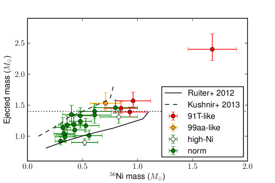
Figure 10: Ejected mass vs. ${}^{56}\mathrm{Ni}$ mass for the SNfactory sample in our fiducial analysis. Colors represent different spectroscopic subtypes, as in Figure 7. The horizontal dotted line marks the Chandrasekhar mass $M=1.4~{}M_{\odot}$. The black solid curve shows the expected $M_{\mathrm{ej}}$-$M_{{}^{56}\mathrm{Ni}}$ relation for sub-Chandrasekhar-mass double detonations from the models of Fink et al. (2010) as presented in Ruiter et al. (2013). The dashed curve shows the predictions of the white dwarf collision model of Kushnir et al. (2013).

Figure 10 shows $M_{\mathrm{ej}}$ vs. $M_{{}^{56}\mathrm{Ni}}$ for the SNfactory data and the expected relations for the models of Ruiter et al. (2013) and Kushnir et al. (2013). The Ruiter et al. (2013) trend seems to be consistent with a few of the lowest-mass SNfactory SNe Ia, but in general the predicted increase of $M_{{}^{56}\mathrm{Ni}}$ with $M_{\mathrm{ej}}$ is too steep to accommodate most of our observations. The trend of Kushnir et al. (2013) does reasonably well for some of the low-$M_{{}^{56}\mathrm{Ni}}$ SNfactory SNe Ia, but can accommodate neither our least massive SNe nor bright 1991T-like SNe Ia. The latter could perhaps be explained by the more detailed collision models of Raskin et al. (2010).

Interestingly, our SNe Ia with $M_{\mathrm{ej}}>1.3~{}M_{\odot}$ lie in a locus parallel to the Ruiter et al. (2013) curve and about 0.3 $M_{\odot}$ higher. While these higher-mass SNe Ia cannot easily be explained by double detonations, they could perhaps be explained more naturally as double-degenerate mergers. The violent merger models of Pakmor et al. (2010, 2011, 2012) are expected to produce similar ${}^{56}\mathrm{Ni}$ yields to double-detonation models with comparable primary white dwarf masses (Ruiter et al., 2013). Reproducing the ${}^{56}\mathrm{Ni}$ masses from our reconstruction requires a primary white dwarf mass of at least 1.1 $M_{\odot}$. However, Pakmor et al. (2011) showed that in violent mergers of two carbon-oxygen white dwarfs, a mass ratio of at least 0.8 is needed to trigger the explosion, meaning that violent mergers with $M_{{}^{56}\mathrm{Ni}}>0.5~{}M_{\odot}$ should have $M_{\mathrm{ej}}>1.9~{}M_{\odot}$, like the different views of 11+09 listed in Table LABEL:tbl:massrecon-mpa (which our method correctly reconstructed as super-Chandrasekhar). Our absolute mass scale would have to be inaccurate at 50% level to explain our observations with current models of violent mergers of two carbon-oxygen white dwarfs. The trend could also be generated by violent mergers of a carbon-oxygen white dwarf with a helium white dwarf (Pakmor et al., 2013), since helium ignites more readily than carbon and a near-equal mass ratio is therefore not necessary. More work is needed to understand whether such mergers with system masses and synthesized ${}^{56}\mathrm{Ni}$ masses consistent with our observations would appear spectroscopically normal.

The simplest explanation is that more massive, more ${}^{56}\mathrm{Ni}$-rich SNe Ia are Chandrasekhar-mass delayed detonations, arising either from slow mergers of double-degenerate systems (Iben & Tutukov, 1984) or from single-degenerate systems. Double-detonation models with $M_{\mathrm{ej}}>1.15~{}M_{\odot}$ have $M_{{}^{56}\mathrm{Ni}}$-$M_{\mathrm{ej}}$ ratios which should result in peculiar spectra. The mean mass of our normal SNe Ia above this threshold (of which there are eight) is $1.31\pm 0.02~{}M_{\odot}$ (stat), within 0.1 $M_{\odot}$ of the Chandrasekhar mass; this increases to $1.36\pm 0.02~{}M_{\odot}$ if the Scalzo et al. (2012) SNe (i.e., other than SN 2007if) are included.

Thus, according to our best current models, the data require at least two progenitor scenarios: one for sub-Chandrasekhar-mass white dwarfs, and one or more for Chandrasekhar-mass and more massive white dwarfs, which could arise from a variety of channels including Chandrasekhar-mass delayed detonations, double-degenerate violent mergers, or possibly spin-down single- or double-degenerate models resulting in a single super-Chandrasekhar-mass white dwarf. Since we have modeled only the bolometric light curves, with no details of the spectroscopic evolution or other observables (such as polarization or evidence for weak CSM interaction), our results should not be taken to prescribe any particular subset of explosion models of a particular mass. However, any successful model or suite of models should be able to reproduce our findings.

6 Conclusions

We have demonstrated a method to reconstruct the ejected masses of normal SNe Ia using Bayesian inference. The method uses the semi-analytic formalism of Jeffery (1999) to compute the predicted late-time bolometric light curve from ${}^{56}\mathrm{Co}$ decay for a SN Ia of a given ejected mass; it is similar to the method of Stritzinger et al. (2006), but includes more realistic near-infrared corrections and more useful priors on unobserved variables. Applying the method to a sample of SNfactory SNe Ia with observations at appropriately late phases, and to a suite of synthetic light curves from full three-dimensional radiation transfer simulations of SNe Ia, we have shown the following:

1. The reconstructed ejecta mass is strongly correlated with the light curve width measured using cosmological light curve fitters, with a slope significantly different from zero. We interpret this as strong evidence for a range of ejected masses in SNe Ia. Even if the range of masses is not as wide as our fiducial reconstruction suggests, due to variation in the density profiles or ${}^{56}\mathrm{Ni}$ distributions which we do not directly constrain, any suite of explosion models intending to explain normal SNe Ia must reproduce this correlation.

2. Our derived values for the ejected mass are relatively insensitive to systematic uncertainties in the ${}^{56}\mathrm{Ni}$ mass, to mild asymmetry in the ejecta, and presumably to any systematic which does not affect the shape of the bolometric light curve. The systematic error in our overall reconstructed mass scale associated with effects we are able to quantify is about $\pm 0.15$ $M_{\odot}$. This gives us further confidence that we are actually constraining the ejected masses of these SNe. Our most influential systematics are the unknown degree of radiation trapping near maximum light (parametrized by $\alpha$) and the influence of the ejecta density profile.

3. Ejected masses can be reconstructed via this method using a single observation of sufficiently high signal-to-noise at +40 days after bolometric maximum light, though with a mild bias towards low masses compared to a reconstruction done with a more complete light curve.

4. The observed locations of our mass estimates in the $M_{\mathrm{ej}}$-$M_{{}^{56}\mathrm{Ni}}$ plane are not all consistent with sub-Chandrasekhar-mass double-detonation models (Fink et al., 2010; Woosley & Kasen, 2011; Ruiter et al., 2013). If these models are taken as representative of sub-Chandrasekhar-mass SN Ia models in general, our results favor at least two progenitor channels for normal SNe Ia.

Although we have learned much from a fairly simple treatment of a fairly small statistical sample of SNe Ia, we should bear in mind the method’s limitations. Semi-analytic treatments are necessarily approximate, with their main advantage being speed. They rely on simplified parametrizations of a number of complex physical effects, and cannot predict the spectra of these events in detail, so that spectroscopic information must be incorporated in a very schematic way. As numerical methods advance and large grids or libraries of synthetic spectra from contemporary explosion models become available, we may learn more by comparing spectra directly to the models (e.g. Blondin et al., 2013a; Dessart et al., 2013). In the meantime, however, some interplay between semi-analytic and full numerical techniques may help us progress, with the former incorporating useful prior information from the latter.

Our specific method assumes spherically symmetric ejecta and simplified functional forms for the radial density profile and the ${}^{56}\mathrm{Ni}$ distribution. Although its performance on strongly asymmetric explosion models with non-exponential density profiles is better at first glance than one might expect, the impact of strong asymmetries or deviations from an exponential density profile on our results are not yet understood in detail. Extensions of the method that incorporate additional information to break the degeneracy between viewing angle and colour or intrinsic brightness (along the lines of, e.g. Maeda et al., 2011), or which marginalize over possible asymmetries, density perturbations, and ${}^{56}\mathrm{Ni}$ distributions to produce a more robust estimate of the systematic error, will help us derive more accurate ${}^{56}\mathrm{Ni}$ masses and ejected masses in the future.

Finally, a larger statistical sample is also highly desirable to replicate our findings and to make further inferences about SN Ia progenitor populations. Applying our method to a larger sample of SNe Ia with good late-time light curves in different host galaxy environments (including, potentially, highly extinguished SNe Ia if NIR data are available to constrain the extinction) should help us validate and calibrate the relations between $M_{\mathrm{ej}}$ and $x_{1}$, and between $M_{\mathrm{ej}}$ and $M_{{}^{56}\mathrm{Ni}}$. Use of these calibrated relations will then allow us to provide mass measurements for a much larger sample of SNe, to determine the true volumetric rates of SNe Ia broken down by ejected mass and as a function of redshift, and ultimately to compare to binary population synthesis models for the progenitor channels of interest. Knowledge of the progenitor mass distribution for large samples of SNe Ia used in future cosmological Hubble diagrams should help to constrain the relative rates of possible progenitor scenarios, thereby improving our understanding both of the dark energy and of the tools we use to study it.

Appendix A Gaussian Process Regression

GP regression is a machine learning technique which can be used to fit smooth curves to data. Rather than specifying a fixed underlying functional form, the curve itself is treated as a stochastic process, such that any two points $x$, $x^{\prime}$ on the curve have a joint Gaussian distribution described by a covariance function $k(x,x^{\prime};\Theta_{i})$; the arguments $\Theta_{i}$ are a set of hyperparameters which encode prior knowledge about the curve (for example, a correlation time-scale between consecutive light curve points) in a Bayesian framework. The hyperparameters can be trained by maximum likelihood estimation, trading off complexity in the model with the residuals of the data from the curve. The process also generalizes to multiple independent variables, or data “features”, and the curves become best-fitting hypersurfaces.

GP regression can be very useful in contexts where the underlying functional form of a relation between data points is not known a priori, but is expected to be smooth. It is easier to apply than conventional Gaussian smoothing to data which are unevenly sampled, such as light curves. Moreover, a GP regression fit can be viewed as a probability distribution in function space, so that each draw from the fit corresponds to a possible realization of the underlying trend which is consistent with the data and satisfies the covariance function $k(x,x^{\prime};\Theta_{i})$ for the best-fit $\Theta_{i}$. This property makes it straightforward to estimate errors on the range of GP predictions at a given value of $x$ by Monte Carlo methods.

We use GP regression in several contexts in the analysis to follow, implemented using the Python module sklearn (Pedregosa et al., 2011).

A.1 Light Curve Fits

For bolometric and single-band light curve fits, we use a squared-exponential covariance function $k(t,t^{\prime})=e^{-0.5(t-t^{\prime})^{2}/\tau^{2}}+\sigma^{2}\delta(t-t^{\prime})$, with a single feature $t$ and two hyperparameters: a correlation time-scale $\tau$ in days, and a “nugget” term $\sigma$ describing the noise (which we fix to be the median 1-$\sigma$ error in magnitudes). While there is a slight variation in the correlation time-scale from SN to SN, as might be expected, we find our data are well-represented by GP fits with $0.5<\tau<2.0$, and fits outside this range generally overfit the data or display pathological behavior; we therefore constrain $\tau$ to lie in this range when fitting light curves.

A.2 Near-Infrared Flux Corrections

For the near-infrared corrections (see §3.2), we fit a GP with three parameters: rest-frame $B$-band phase $t$, wavelength $\log\ \lambda$, and SALT2 $x_{1}$ (i.e., decline rate). Near-infrared light curves show a characteristic second maximum occurring between 25 and 35 days after $B$-band maximum light, the timing of which correlates strongly with the $B$-band decline rate (Folatelli et al., 2010). Slower-declining SNe Ia have later-occurring NIR second maxima, which can be understood in terms of a model in which the second maximum is powered by the recombination of Fe 3 to Fe 2, which redistributes flux from bluer wavelengths into the NIR (Kasen, 2006). Accounting for the dependence of the NIR behavior on decline rate can make a difference of nearly 1 mag in $Y$ and $J$ at 40 days after $B$-band maximum light. We also allow for correlation between neighboring bands through the wavelength parameter, with each band represented at its central wavelength. While the $YJHK$ bands represent statistically independent measurements, they have qualitatively similar behavior arising from a common physical origin, and capturing the similarities in the GP fit can help improve the statistical power of the GP prediction in each band. The covariance function is

$$k({\bf x},{\bf x}^{\prime})=\exp\left[({\bf x}-{\bf x}^{\prime})^{T}{\bf\Theta}({\bf x}-{\bf x}^{\prime})^{T}\right],$$ (10)

where the feature vector is ${\bf x}=(t,x_{1},\log(\lambda))$ and the hyperparameters are ${\bf\Theta}=\mathrm{diag}(\Theta_{t},\Theta_{x_{1}},\Theta_{\lambda})$.

Although the CSP data also show some variation in the contrast of the NIR second maximum, possibly correlating with different degrees of mixing of ${}^{56}\mathrm{Ni}$ in the outer layers of ejecta (Kasen, 2006; Folatelli et al., 2010), this behavior has little influence on the NIR light curve after the second maximum. We therefore do not attempt to capture such variation here, since our modeling in §4 requires accurate predictions only of the behavior at maximum light (${}^{56}\mathrm{Ni}$ mass) and at phases after the NIR second maximum.

References

- (1)
- Aldering et al. (2002) Aldering, G., Adam, G., Antilogus, P., et al. 2002, Proc. SPIE, 4836, 61
- Aldering et al. (2006) Aldering, G., Antilogus, P., Bailey, S., et al. 2006, ApJ, 650, 510
- Arnett (1982) Arnett, W. D. 1982, ApJ, 253, 785
- Bacon et al. (1995) Bacon, R., Adam, G., Baranne, A., et al. 1995, A&AS, 113, 347
- Bacon et al. (2000) Bacon, R., Emsellem, E., Copin, Y., et al. 2000, in ASP Conf. Ser. 195, Imaging the Universe in Three Dimensions, ed. W. van Breugel & J. Bland-Hawthorn (San Francisco: ASP), 173
- Bacon et al. (2001) Bacon, R., Copin, Y., Monnet, G., et al. 2001, MNRAS, 326, 23
- Bailey et al. (2009) Bailey, S., Aldering, G., Antilogus, P., et al. 2009, A&A, 500, L17
- Baltay et al. (2007) Baltay, C., Rabinowitz, D., Andrews, P., et al. 2007, PASP, 119, 1278
- Benz et al. (1989) Benz, W., Thielemann, F.-K., & Hills, J. G. 1989, ApJ, 342, 986
- Blondin & Tonry (2007) Blondin, S., & Tonry, J. L. 2007, ApJ, 666, 1024
- Blondin et al. (2011) Blondin, S., Kasen, D., Roepke, F., et al. 2011, MNRAS, 417, 1280
- Blondin et al. (2013a) Blondin, S., Dessart, L., Hillier, D. J., et al. 2013, MNRAS, 429, 2127
- Bloom et al. (2012) Bloom, J. S., Kasen, D., Shen, K. J., et al. 2012, ApJ, 744, L17
- Bohlin & Gilliland (2004) Bohlin, R. C., & Gilliland, R. L. 2004, AJ, 127, 3508
- Bongard et al. (2011) Bongard, S., Soulez, F., Thiébaut, É. et al. 2011, MNRAS, 418, 258
- Branch et al. (1993) Branch, D., Fisher, A., & Nugent, P. 1993, AJ, 106, 2383
- Buton et al. (2013) Buton, C., Copin, Y., Aldering, G., et al. 2013, A&A, 549, A8
- Cano et al. (2013) Cano, Z. 2013, MNRAS, 434, 1098
- Cardelli et al. (1988) Cardelli, J. A., Clayton, G. C. & Mathis, J. S. 1988, ApJ, 329, L33
- Childress et al. (2013) Childress, M. J., Aldering, G., Antilogus, P., et al. 2013, ApJ, 770, 107
- Dessart et al. (2013) Dessart, L., Hillier, D. J., Blondin, S., et al. 2013, MNRAS, submitted (arXiv:1308.6352)
- Di Stefano & Kilic (2012) Di Stefano, R. & Kilic, M. 2012, ApJ, 759, 56
- Drout et al. (2011) Drout, M. R., Soderberg, A. M., Gal-Yam, A., et al. 2011, ApJ, 741, 97
- Fink et al. (2010) Fink, M., Röpke, F. K., Hillebrandt, W., et al.2010, A&A, 514, A53
- Folatelli et al. (2010) Folatelli, G., Phillips, M. M., Burns, C., R., et al. 2010, AJ, 139, 120
- Folatelli et al. (2011) Folatelli, G., Phillips, M. M., Morell, N., et al. 2011, ApJ, 745, 74
- Foley & Kasen (2010) Foley, R. J. & Kasen, D. 2010, ApJ, 729, 55
- Foreman-Mackey et al. (2013) Foreman-Mackey, D., et al.2013, PASP, 125, 306
- Ganeshalingam et al. (2011) Ganeshalingam, M., Li, W., & Filippenko, A. V. 2011, MNRAS, 416, 2607
- Goldhaber et al. (2001) Goldhaber, G., Groom, D. E., Kim, A. G., et al. 2001, ApJ, 558, 359
- Guy et al. (2007) Guy, J., Astier, P., Baumont, S., et al. 2007, A&A, 466, 11
- Guy et al. (2010) Guy, J., Sullivan, M., Conley, A., et al. 2010, A&A, 523, 7
- Hachisu et al. (2011) Hachisu, I., Kato, M., Saio, H., et al.2012, ApJ, 744, 69
- Han & Podsiadlowski (2004) Han, Z., & Podsiadlowski, P. 2004, MNRAS, 350, 1301
- Hicken et al. (2009) Hicken, M., Wood-Vasey, M. W., Blondin, S., et al. 2009, ApJ, 700, 1097
- Höflich & Khohklov (1996) Höflich, P. & Khohklov, A. 1996, ApJ, 457, 500
- Howell et al. (2005) Howell, D. A., Sullivan, M., Perrett, K., et al. 2005, ApJ, 634, 1190
- Howell et al. (2006) Howell, D. A., Sullivan, M., Nugent, P. E., et al. 2006, Nature, 443, 308
- Howell et al. (2009) Howell, D. A., Sullivan, M., Brown, E. F., et al. 2009, ApJ, 691, 661
- Iben & Tutukov (1984) Iben, I. & Tutukov, A. V. 1984, ApJS, 54, 335
- Jeffery (1999) Jeffery, D. J. 1999, arXiv:astro-ph/9907015
- Jeffery, Branch, & Baron (2006) Jeffery, D. J., Branch, D., & Baron, E. 2006, arXiv:astro-ph/0609804
- Justham (2011) Justham, S. 2011, ApJ, 730, L34
- Kasen (2006) Kasen, D. 2006, ApJ, 649, 939
- Katz & Dong (2012) Katz, B. & Dong, S. 2012, arXiv:1211.4584
- Kessler et al. (2009) Kessler, R. et al. 2009, ApJS, 185, 32
- Khokhlov et al. (1993) Khokhlov, A., Müller, E. & Höflich, P. 1993, A&A, 270, 223
- Kromer & Sim (2009) Kromer, M., & Sim, S. A. 2009, MNRAS, 398, 1809
- Kromer et al. (2010) Kromer, M., Sim, S. A., Fink, M., et al.2010, ApJ, 719, 1067
- Kromer et al. (2013) Kromer, M., Fink, M., Stanishev, V., et al.2013, MNRAS, 429, 2287
- Krueger et al. (2010) Krueger, B. K. Jackson, A. P., Townsley, D. M., et al.2010, ApJ, 719, L5
- Krueger et al. (2012) Krueger, B. K. Jackson, A. P., Townsley, D. M., et al.2012, ApJ, 757, 175
- Kushnir et al. (2013) Kushnir, D., Katz, B., Dong, S., et al. 2013, ApJ, 778, L37
- Lantz et al. (2004) Lantz, B., Aldering, G., Antilogus, P., et al. 2004, Proc. SPIE, 5249, 146
- Lepage (1978) Lepage, G. P. 1978, Journal of Computational Physics, 27, 192
- Linder (2006) Linder, E. V. 2006, Phys. Rev. D, 74, 103518
- Madison et al. (2005) Madison, D. R., Baek, M., Li, W., 2005, CBET 233, 1.
- Maeda & Iwamoto (2009) Maeda, K., & Iwamoto, K. 2009, MNRAS, 394, 239
- Maeda et al. (2011) Maeda, K., Leloudas, S., Taubenberger, S., et al. 2011, MNRAS, 413, 3075
- Mazzali et al. (2007) Mazzali, P. A., Roepke, F., Benetti, S., et al. 2007, Science, 315, 825
- Nomoto et al. (1984) Nomoto, K., Thielemann, F.-K., & Yokoi, K. 1984, ApJ, 286, 644
- Nomoto & Kondo (1991) Nomoto, K. & Kondo, Y. 1991, ApJ, 367, L19
- Nugent et al. (1995) Nugent, P., Branch, D., Baron, E., et al. 1995, Phys. Rev. Lett., 75, 394
- Nugent et al. (2009) Nugent, P., Sullivan, M., Howell, D. A., et al.2009, ATEL, 2174, 1.
- Nugent et al. (2011) Nugent, P., Sullivan, M., Howell, D. A., et al.2011, CBET, 2792, 1.
- Nugent et al. (2011) Nugent, P., Sullivan, M., Cenko, S. B., et al. 2011, Nature, 480, 344
- Orff & Newton (2007) T. Orff, J. Newton, CBET 983, 1 (2007).
- Pakmor et al. (2010) Pakmor, R., Kromer, M., Röpke, F. K., et al.2010, Nature, 463, 61
- Pakmor et al. (2011) Pakmor, R., Hachinger, S., Röpke, F. K., et al.2011, A&A, 528, 117
- Pakmor et al. (2012) Pakmor, R., Kromer, M., & Taubenberger, S. 2013, ApJ, 747, L10
- Pakmor et al. (2013) Pakmor, R., Kromer, M., Taubenberger, S., et al.2013, ApJ, 770, L8
- Pedregosa et al. (2011) Pedregosa, F., Varoquaux, G., Gramfort, A., et al.2011, Journal of Machine Learning Research, 12, 2825
- Perlmutter et al. (1999) Perlmutter, S., Aldering, G., Goldhaber, G., et al. 1999, ApJ, 517, 565
- Phillips et al. (1999) Phillips, M. M., Lira, P., Suntzeff, N. B., et al. 1999, AJ, 118, 1766
- Phillips et al. (2007) Phillips, M. M., Li, W., Frieman, J. A., et al. 2007, PASP, 119, 360
- Poznanski et al. (2012) Poznanski, D., Prochaska, J. X., & Bloom, J. S. 2012, MNRAS, 426, 1465
- Raskin et al. (2009) Raskin, C., Timmes, F. X., Scannapieco, E., et al. 2009, MNRAS, 399, L156
- Raskin et al. (2010) Raskin, C., Scannapieco, E., Rockefeller, G., et al. 2010, ApJ, 724, 111
- Rasmussen & Williams (2006) Rasmussen, C. E. & Williams, C. K. I., 2006, Gaussian Processes for Machine Learning, MIT Press
- Rex et al. (2007) Rex, J., Li, W., Filippenko, A. V., et al. 2008, CBET 1437, 1.
- Riess et al. (1996) Riess, A. G., Press, W. H., & Kirshner, R. P. 1996, ApJ, 473, 88
- Riess et al. (1998) Riess, A. G., Filippenko, A. V., Challis, P., et al. 1998, AJ, 116, 1009
- Rosswog et al. (2009) Rosswog, S., Kasen, D., Guillochon, J., et al. 2009, ApJ, 705, 128
- Ruiter et al. (2011) Ruiter, A. J., Belczynski, K., Sim, S. A., et al. 2011, MNRAS, 417, 408
- Ruiter et al. (2013) Ruiter, A. J., Sim, S. A., Pakmor, R., et al. 2013, MNRAS, 429, 1425
- Scalzo et al. (2010) Scalzo, R. A., Aldering, G., Antilogus, P., et al. 2010, ApJ, 713, 1073
- Scalzo et al. (2012) Scalzo, R. A., Aldering, G., Antilogus, P., et al. 2012, ApJ, 757, 12
- Schlegel et al. (1998) Schlegel, D. J., Finkbeiner, D. P. & Davis, M. 1998, ApJ, 500, 525
- Seitenzahl et al. (2009) Seitenzahl, I., Meakin, C. A., Townsley, D. M., et al. 2009, ApJ, 696, 515
- Seitenzahl et al. (2011) Seitenzahl, I., Ciaraldi-Schoolmann, F., & Röpke, F. K. 2011, MNRAS, 414, 2709
- Seitenzahl et al. (2013) Seitenzahl, I., Ciaraldi-Schoolmann, F., Röpke, F. K., et al. 2013, MNRAS, 429, 1156
- Silverman et al. (2011) Silverman, J. M. et al. 2011, MNRAS, 410, 585
- Sim et al. (2010) Sim, S. A., Röpke, F. K., Hillebrandt, W., et al. 2010, ApJ, 714, L52
- Sim et al. (2012) Sim, S. A., Fink, M., Kromer, M., et al. 2012, MNRAS, 420, 3003
- Stritzinger et al. (2006) Stritzinger, M., Leibundgut, B., Walch, S., et al. 2006, A&A, 450, 241
- Stritzinger et al. (2011) Stritzinger, M., Phillips, M. M., Boldt, L. N., et al. 2011, AJ, 142, 156
- Sullivan et al. (2011) Sullivan, M., Kasliwal, M. M., Nugent, P. E., et al.2011, ApJ, 732, 118
- Sullivan et al. (2011) Sullivan, M., Guy, J., Conley, A., et al.2011, ApJ, 737, 102
- Suzuki et al. (2012) Suzuki, N., Rubin, D., Lidman, C., et al.2012, ApJ, 746, 85
- Swartz et al. (1995) Swartz, D. A., Sutherland, P. G., & Harkness, R. P. 1995, ApJ, 446, 766
- Taubenberger et al. (2011) Taubenberger, S., Benetti, S., Childress, M. et al. 2011, MNRAS, 412, 2735
- Thomas et al. (2007) Thomas, R. C., Aldering, G., Antilogus, P., et al. 2007, ApJ, 654, 53
- Thomas et al. (2011) Thomas, R. C., Aldering, G., Antilogus, P., et al. 2011, ApJ, 743, 27
- Tripp (1998) Tripp, R. 1998, A&A, 331, 815
- Turatto et al. (2002) Turatto, M., Benetti, S., & Cappellaro, E. 2002, arXiv:astro-ph/0211219
- van Kerkwijk et al. (2010) van Kerkwijk, M., Chang, P., & Justham, S. 2010, ApJ, 722, L157
- Wang et al. (2009) Wang, X., Filippenko, A. V., Ganeshalingam, M., et al. 2009, ApJ, 699, L139
- Wang & Han (2012) Wang, B., & Han, Z. 2012, New Astronomy Reviews, 56, 122
- Whelan & Iben (1973) Whelan, J. & Iben, I. J. 1973, ApJ, 186, 1007
- Woosley & Weaver (1994) Woosley, S. E. & Weaver, T. A. 1994, ApJ, 423, 371
- Woosley & Kasen (2011) Woosley, S. E. & Kasen, D. 2011, ApJ, 734, 38
- Yoon & Langer (2005) Yoon, S.-C. & Langer, N. 2005, A&A, 435, 967
- Yuan et al. (2010) Yuan, F., Quimby, R. M., Wheeler, J. C., et al. 2010, ApJ, 715, 1338