Infinitesimal Perturbation Analysis for Quasi-Dynamic Traffic Light Controllers

Abstract

We consider the traffic light control problem for a single intersection modeled as a stochastic hybrid system. We study a quasi-dynamic policy based on partial state information defined by detecting whether vehicle backlogs are above or below certain controllable thresholds. Using Infinitesimal Perturbation Analysis (IPA), we derive online gradient estimators of a cost metric with respect to these threshold parameters and use these estimators to iteratively adjust the threshold values through a standard gradient-based algorithm so as to improve overall system performance under various traffic conditions. Results obtained by applying this methodology to a simulated urban setting are also included.

1 Introduction

The Traffic Light Control (TLC) problem consists of adjusting green and red light cycles in order to control the traffic flow through an intersection and, more generally, through a set of intersections and traffic lights. The ultimate objective is to minimize congestion (hence delays experienced by drivers) at a particular intersection, as well as an entire area consisting of multiple intersections with traffic lights. Recent technological developments have made it possible to collect and process traffic data so that they may be applied in solving the TLC problem in real time. Fundamentally, TLC is a form of scheduling for systems operating through simple switching control actions. Numerous solution algorithms have been proposed and we briefly review some of them. Porche et al. (1996) used a decision tree model with a Rolling Horizon Dynamic Programming (RHDP) approach, while Dujardin et al. (2011) proposed a multiobjective Mixed Integer Linear Programming (MILP) formulation. Optimal TLC was also stated as a special case of an Extended Linear Complementarity Problem (ELCP) by De Schutter (1999), and formulated as a hybrid system optimization problem by Zhao and Chen (2003). Yu and Recker (2006) modeled a traffic light intersection as a Markov Decision Process (MDP) and a game theoretic approach was applied to a finite controlled Markov chain model by Alvarez and Poznyak (2010). Relying on sensor information regarding traffic congestion, Choi et al. (2002) developed a first-order Sugeno fuzzy model and incorporated it into a fuzzy logic controller. Perturbation analysis techniques were used by Head et al. (1996) and Fu and Howell (2003) for modeling a traffic light intersection as a stochastic Discrete Event System (DES), while an Infinitesimal Perturbation Analysis (IPA) approach, using a Stochastic Flow Model (SFM) to represent the queue content dynamics of roads at an intersection, was presented in [Panayiotou et al. (2005)].

Our work is also based on modeling traffic flow through an intersection controlled by switching traffic lights as an SFM, which conveniently captures the system’s inherent hybrid nature: while traffic light switches exhibit event-driven dynamics, the flow of vehicles through an intersection is best represented through time-driven dynamics. In [Geng and Cassandras (2012)], IPA was applied with respect to controllable green and red cycle lengths for a single isolated intersection and in [Geng and Cassandras (2013a)] for multiple intersections. Traffic flow rates need not be restricted to take on deterministic values, but may be treated as stochastic processes (see [Cassandras et al. (2002)]), which are suited to represent the continuous and random variations in traffic conditions. Using the general IPA theory for Stochastic Hybrid Systems (SHS) in [Wardi et al. (2010)] and [Cassandras et al. (2010)], on-line gradients of performance measures are estimated with respect to several controllable parameters with only minor technical conditions imposed on the random processes that define input and output flows. These IPA estimates have been shown to be unbiased, even in the presence of blocking due to limited resource capacities and of feedback control (see [Yao and Cassandras (2011)]). It should be emphasized that IPA is not used to estimate performance measures, but only their gradients, which may be subsequently incorporated into standard gradient-based algorithms in order to effectively control parameters of interest.

In contrast to earlier work where the adjustment of light cycles did not make use of real-time state information, Geng and Cassandras (2013b) proposed a quasi-dynamic control setting in which partial state information is used conditioned upon a given queue content threshold being reached. In this paper, we draw upon this setting, but rather than controlling the light cycle lengths as in [Geng and Cassandras (2013b)], here we focus on the threshold parameters and derive IPA performance measure estimators necessary to optimize these parameters, while assuming fixed cycle lengths. Our goal is to compare the relative effects of the threshold parameters and the light cycle length parameters on our objective function, build upon these results, and ultimately control both the light cycle lengths and the queue content thresholds simultaneously.

In Section 2, we formulate the TLC problem for a single intersection and present the modeling framework used throughout our analysis for controlling vehicle queue thresholds. Section 3 details the derivation of an IPA estimator for the cost function gradient with respect to a controllable parameter vector defined by these thresholds. The IPA estimator is then incorporated into a gradient-based optimization algorithm and we include simulation results in Section 4, showing how the proposed quasi-dynamic control offers considerable improvement over prior results.

2 Problem Formulation

The system we consider comprises a single intersection, as shown in Fig. 1. For simplicity, left-turn and right-turn traffic flows are not considered and yellow light cycles are implicitly accounted for within a red light cycle. We assign to each queue $i$ a guaranteed minimum GREEN cycle length $\theta_{i,\min}$, and a maximum length $\theta_{i,\max}$ which (in contrast to [Geng and Cassandras (2013b)]) we assume to be fixed. We define a state vector $x(t)=[x_{1}(t),x_{2}(t)]$ where $x_{i}(t)\in\mathbb{R}^{+}$ is the content of queue $i$. For each queue $i$, we also define a “clock” state variable $z_{i}(t)$, $i=1,2$, which measures the time since the last switch from RED to GREEN of the traffic light for queue $i$, so that $z_{i}(t)\in[0,\theta_{i,\max}]$. Setting $z(t)=[z_{1}(t),z_{2}(t)]$, the complete system state vector is $[x(t),z(t)]$. Within the quasi-dynamic setting considered in this work, the controllable parameter vector of interest is given by $\mathbf{s}=\left[s_{1},s_{2}\right]$, where $s_{n}\in\Re^{+}$ is a queue content threshold value for road $n=1,2$. The notation $x(\mathbf{s},t)=[x_{1}(\mathbf{s},t),x_{2}(\mathbf{s},t)]$ is used to stress the dependence of the state on these threshold parameters. However, for notational simplicity, we will henceforth write $x(t)$ when no confusion arises; the same applies to $z(t)$.

Let us now partition the queue content state space into the following four regions:

$$X_{0}=\{(x_{1},x_{2}):x_{1}(t)<s_{1},\text{ }x_{2}(t)<s_{2}\}$$

$$X_{1}=\{(x_{1},x_{2}):x_{1}(t)<s_{1},\text{ }x_{2}(t)\geq s_{2}\}$$

$$X_{2}=\{(x_{1},x_{2}):x_{1}(t)\geq s_{1},\text{ }x_{2}(t)<s_{2}\}$$

$$X_{3}=\{(x_{1},x_{2}):x_{1}(t)\geq s_{1},\text{ }x_{2}(t)\geq s_{2}\}$$

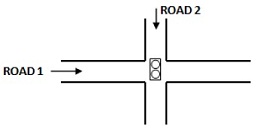
Figure 1: A single traffic light intersection with two cross-roads

At any time $t$, the feasible control set for the traffic light controller is $U=\{1,2\}$ and the control is defined as:

$$u\left(x(t),z(t)\right)\equiv\left\{\begin{array}[c]{c}1\\ 2\end{array}\right.\begin{array}[c]{l}\text{i.e., set road }1\text{ GREEN, road }2\text{ RED}\\ \text{i.e., set road }2\text{ GREEN, road }1\text{ RED}\end{array}$$ (1)

A dynamic controller is one that makes full use of the state information $z(t)$ and $x(t)$. Obviously, $z(t)$ is the controller’s known internal state, but the queue content state is generally not observable. We assume, however, that it is partially observable. Specifically, we can only observe whether $x_{i}(t)$ is below or above some threshold $s_{i},i=1,2$ (this is consistent with actual traffic systems where sensors (typically, inductive loop detectors) are installed at each road near the intersection). In this context, we shall define a quasi-dynamic controller of the form $u\left(X(t),z(t)\right)$, with $X(t)\in\left\{X_{0},X_{1},X_{2},X_{3}\right\}$, as follows:

For $X(t)\in\left\{X_{0},X_{3}\right\}$:

$$u\left(z(t)\right)=\left\{\begin{array}[c]{c}1\\ 2\end{array}\right.\begin{array}[c]{l}\text{if }z_{1}(t)\in\left(0,\theta_{1,\max}\right)\text{ and }z_{2}(t)=0\\ \text{otherwise}\end{array}$$ (2)

For $X(t)=X_{1}$:

$$u\left(z(t)\right)=\left\{\begin{array}[c]{c}1\\ 2\end{array}\right.\begin{array}[c]{l}\text{if }z_{1}(t)\in\left(0,\theta_{1,\min}\right)\text{ and }z_{2}(t)=0\\ \text{otherwise}\end{array}$$ (3)

For $X(t)=X_{2}$:

$$u\left(z(t)\right)=\left\{\begin{array}[c]{c}2\\ 1\end{array}\right.\begin{array}[c]{l}\text{if }z_{2}(t)\in\left(0,\theta_{2,\min}\right)\text{ and }z_{1}(t)=0\\ \text{otherwise}\end{array}$$ (4)

This is a simple form of hysteresis control to ensure that the $i$th traffic flow always receives a minimum GREEN light cycle $\theta_{i,\min}$. Clearly, the GREEN light cycle may be dynamically interrupted anytime after $\theta_{i,\min}$ based on the partial state feedback provided through $X(t)$. For instance, if a transition into $X_{1}$ occurs while $u\left(X(t),z(t)\right)=1$ and $z_{1}(t)>\theta_{1,\min}$, then the light switches from GREEN to RED for road 1 in order to accommodate an increasing backlog at road 2. For notational simplicity, we will write $u(t)$ when no confusion arises, as we do with $x(t)$, $z(t).$

The stochastic processes involved in this system are defined on a common probability space $\left(\Omega,F,P\right)$. The arrival flow processes are $\{\alpha_{n}(t)\}$, $n=1,2$, where $\alpha_{n}(t)$ is the instantaneous vehicle arrival rate at time $t$. The departure flow process on road $n$ is defined as:

$$\beta_{n}(t)=\left\{\begin{array}[c]{l}h_{n}(X(t),z(t),t)\\ \alpha_{n}(t)\\ 0\end{array}\right.\begin{array}[c]{l}\text{if }x_{n}(t)>0\text{ and }u(t)=n\\ \text{if }x_{n}(t)=0\text{ and }u(t)=n\\ \text{otherwise}\end{array}$$ (5)

where $h_{n}(X(t),z(t),t)$ is the instantaneous vehicle departure rate at time $t$; for notational simplicity, we will write $h_{n}(t)$ when no confusion arises. We can now write the dynamics of the state variables $x_{n}(t)$ and $z_{n}(t)$ as follows, where we adopt the notation $\overline{n}$ to denote the index of the road perpendicular to road $n=1,2$, and note that the symbols $t^{+}$ ($t^{-}$, respectively) denote the time instant immediately following (preceding, respectively) time $t$:

$$\overset{\cdot}{x}_{n}(t)=\left\{\begin{array}[c]{l}\alpha_{n}(t)\\ 0\\ \alpha_{n}(t)-h_{n}(t)\end{array}\right.\begin{array}[c]{l}\text{if }z_{n}(t)=0\\ \text{if }x_{n}(t)=0\text{ and }\alpha_{n}(t)\leq h_{n}(t)\\ \text{otherwise}\end{array}$$ (6)

$$\overset{\cdot}{z}_{n}(t)=\left\{\begin{array}[c]{c}1\\ 0\end{array}\right.\begin{array}[c]{l}\text{if }z_{\overline{n}}(t)=0\\ \text{otherwise}\end{array}$$ (7)

$$\begin{array}[t]{l}z_{n}(t^{+})=0\\ \text{if }z_{n}(t)=\theta_{n,\max}\\ \text{or }z_{n}(t)=\theta_{n,\min},\text{ }x_{n}(t)<s_{n},\text{ }x_{\overline{n}}(t)\geq s_{\overline{n}}\\ \text{or }z_{n}(t)>\theta_{n,\min},\text{ }x_{n}(t^{-})>s_{n},x_{n}(t^{+})=s_{n},x_{\overline{n}}(t)\geq s_{\overline{n}}\\ \text{or }z_{n}(t)>\theta_{n,\min},\text{ }x_{n}(t)<s_{n},x_{\overline{n}}(t^{-})<s_{\overline{n}},x_{\overline{n}}(t^{+})=s_{\overline{n}}\end{array}$$

In this context, the traffic light intersection in Fig. 1 can be viewed as a hybrid system in which the time-driven dynamics are given by (6)-(7) and the event-driven dynamics are associated with light switches and with events that cause the value of $x_{n}(t)$ to change from strictly positive to zero or vice-versa. It is then possible to derive a Stochastic Hybrid Automaton (SHA) model as in [Geng and Cassandras (2013b)] containing 14 modes, which are defined by combinations of $x_{n}(t)$ and $z_{n}(t)$ values. The event set for this SHA is $\Phi_{n}=\left\{e_{1},e_{2},e_{3},e_{4},e_{5},e_{6},e_{7}\right\}$, where $e_{1}$ is the guard condition $\left[x_{n}=s_{n}\text{ from below}\right]$; $e_{2}$ is the guard condition $\left[x_{n}=s_{n}\text{ from above}\right]$; $e_{3}$ is the guard condition $\left[z_{n}=\theta_{n,\min}\right]$; $e_{4}$ is the guard condition $\left[z_{n}=\theta_{n,\max}\right]$; $e_{5}$ is the guard condition $\left[x_{n}=0\text{ from above}\right]$; $e_{6}$ is a switch in the sign of $\alpha_{n}(t)-h_{n}(t)$ from non-positive to strictly positive; $e_{7}$ is a switch in the sign of $\alpha_{n}(t)$ from 0 to strictly positive. Note that $e_{1},\ldots,e_{4}$ are the events that induce light switches and, for easier reference, we rename them as $\zeta_{n}$, $\gamma_{n}$, $\lambda_{n}$, and $\mu_{n}$, respectively, where the subscript $n$ refers to the road where the event occurred. If we label light switching events from RED to GREEN and GREEN to RED as $R2G_{n}$ and $G2R_{n}$, respectively, we can specify the following rules for our hysteresis-based controller:

Rule 1

The occurrence of event $\zeta_{n}$, while $z_{\overline{n}}>\theta_{\bar{n},\min}$ and $x_{\overline{n}}<s_{\overline{n}}$, results in event $R2G_{n}$.

Rule 2

The occurrence of event $\gamma_{n}$, while $z_{n}>\theta_{n,\min}$ and $x_{\overline{n}}\geq s_{\overline{n}}$, results in event $G2R_{n}$.

Rule 3

The occurrence of event $\lambda_{n}$, while $x_{n}<s_{n}$ and $x_{\overline{n}}\geq s_{\overline{n}}$, results in event $G2R_{n}$.

Rule 4

The occurrence of event $\mu_{n}$ always results in event $G2R_{n}$.

A partial state transition diagram defined in terms of the aggregate queue content states $X(t)$ is shown in Fig. 2. A complete state transition diagram for this SHA is too complicated to draw and is not necessary for IPA, which focuses on analyzing a typical sample path and observable events in it, as shown in Fig. 3. Observe that any such sample path consists of alternating Non-Empty Periods (NEPs) and Empty Periods (EPs), which correspond to time intervals when $x_{n}(t)>0$ (i.e., queue $n$ is non-empty) and $x_{n}(t)=0$ (i.e., queue $n$ is empty), respectively. Let us then label the events corresponding to the end and to the start of an NEP as $E_{n}$ and $S_{n}$, respectively, and note that $E_{n}$ is induced by event $e_{5}$, while $S_{n}$ may be induced by events $e_{6}$ or $e_{7}$ or $G2R_{n}$.

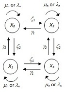
Figure 2: Stochastic Hybrid Automaton for aggregate states $X(t)$ under quasi-dynamic control

Let us denote the $m$th NEP in a sample path of queue $n$, by $\left[\xi_{n,m},\eta_{n,m}\right)$, where $\xi_{n,m}$, $m=1,2,\ldots$, is the time of occurrence of the $m$th $S_{n}$ event and $\eta_{n,m}$ is the time of occurrence of the $m$th $E_{n}$ event, as illustrated in Fig. 3. Additionally, let the time of a light switching event (either $R2G_{n}$ or $G2R_{n}$) within the $m$th NEP be denoted by $t_{n,m}^{j}$, $j=1,...,J_{m}$.

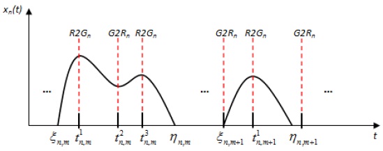
Figure 3: Typical sample path of a traffic light queue

Recall that the purpose of our analysis is to apply IPA to sample path data in order to obtain unbiased gradient estimates of a system performance measure with respect to the controllable parameter vector $\mathbf{s}$ and subsequently incorporate such estimates into a gradient-based optimization scheme. In particular, we define a sample function which measures a weighted mean of the queue lengths over a fixed time interval $[0,T]$:

$$L\left(\mathbf{s};x(0),z(0),T\right)=\frac{1}{T}\underset{n=1}{\overset{2}{\sum}}{\displaystyle\int\limits_{0}^{T}}w_{n}x_{n}\left(\mathbf{s},t\right)dt$$ (8)

where $w_{n}$ is a weight associated with road $n$, and $x(0)$, $z(0)$ are given initial conditions. Since $x_{n}(t)=0$ during EPs of road $n$,(8) can be rewritten as

$$L\left(\mathbf{s};x(0),z(0),T\right)=\frac{1}{T}\overset{2}{\underset{n=1}{\sum}}\underset{m=1}{\overset{M_{n}}{\sum}}{\displaystyle\int\limits_{\xi_{n,m}}^{\eta_{n,m}}}w_{n}x_{n}\left(\mathbf{s},t\right)dt$$ (9)

where $M_{n}$ is the total number of NEPs during the sample path of road $n$. Finally, using $E$ to denote the usual expectation operator, let us define the overall performance metric as

$$J\left(\mathbf{s};x(0),z(0),T\right)=E\left[L\left(\mathbf{s};x(0),z(0),T\right)\right]$$ (10)

We note that it is not possible to derive a closed-form expression of $J\left(\mathbf{s};x(0),z(0),T\right)$ without full knowledge of the processes $\{\alpha_{n}(t)\}$ and $\{\beta_{n}(t)\}$. On the other hand, by assuming only that $\alpha_{n}(t)$ and $\beta_{n}(t)$ are piecewise continuous w.p. 1, we can successfully apply the IPA methodology developed for general SHS by Cassandras et al. (2010) and obtain an estimate of $\nabla J\left(\mathbf{s}\right)$ by evaluating the sample gradient $\nabla L\left(\mathbf{s}\right)$. As we will see, no explicit knowledge of $\alpha_{n}(t)$, $\beta_{n}(t)$ is necessary to estimate $\nabla J\left(\mathbf{s}\right)$, which can then be used to improve current operating conditions or (under certain conditions) to compute an optimal $\mathbf{s}^{\ast}$ through an iterative optimization algorithm of the form

$$s_{i,l+1}=s_{i,l}-\rho_{l}H_{i,l}\left(\mathbf{s}_{l},x(0),T,\omega_{l}\right)$$ (11)

where $\rho_{l}$ is the step size at the $l$th iteration, $l=0,1,...$, and $\omega_{l}$ denotes a sample path from which data are extracted and used to compute $H_{i,l}\left(\mathbf{s}_{l},x(0),T,\omega_{l}\right)$, which is an estimate of $dJ/ds_{i}$. We will further assume that that the derivatives $dL/ds_{i}$ exist w.p. 1 for all $s_{i}\in\Re^{+}$. It is also easy to check that $L\left(\mathbf{s}\right)$ is Lipschitz continuous for $s_{i}\in\Re^{+}$. Under these conditions, it has been shown by Cassandras et al. (2010) that $dL/ds_{i}$ is an unbiased estimator of $dJ/ds_{i}$, $i=1,2$.

3 Infinitesimal Perturbation Analysis

For the sake of completeness we begin with a brief overview of the generalized IPA framework developed for SHS in [Cassandras et al. (2010)]). Consider a sample path of the system over $\left[0,T\right]$ and denote the time of occurrence of the $k$th event (of any type) by $\tau_{k}\left(\theta\right)$, where $\theta$ is a scalar (for simplicity) controllable parameter of interest. We shall also denote the state and event time derivatives with respect to parameter $\theta$ as $x^{\prime}(\theta,t)\equiv\frac{\partial x(\theta,t)}{\partial\theta}$ and $\tau_{k}^{\prime}(\theta)\equiv\frac{\partial\tau_{k}\left(\theta\right)}{\partial\theta}$, respectively, for $k=1,...,N$. The dynamics of $x(\theta,t)$ are fixed over any interevent interval $[\tau_{k}(\theta),\tau_{k+1}(\theta))$ and we write $\dot{x}(\theta,t)=f_{k}(\theta,x,t)$ to represent the state dynamics over this interval. Although we include $\theta$ as an argument in the expressions above to stress dependence on the controllable parameter, we will subsequently drop this for ease of notation as long as no confusion arises. It is shown in [Cassandras et al. (2010)] that the state derivative satisifies

$$\frac{d}{dt}x^{\prime}(t)=\frac{\partial f_{k}(t)}{\partial x}x^{\prime}(t)+\frac{\partial f_{k}(t)}{\partial\theta}$$ (12)

with the following boundary condition:

$$x^{\prime}(\tau_{k}^{+})=x^{\prime}(\tau_{k}^{-})+\left[f_{k-1}(\tau_{k}^{-})-f_{k}(\tau_{k}^{+})\right]\cdot\tau_{k}^{\prime}$$ (13)

Knowledge of $\tau_{k}^{\prime}$ is, therefore, needed in order to evaluate (13). Following the framework in [Cassandras et al. (2010)], there are three types of events for a general stochastic hybrid system. $(i)$ Exogenous Events. These events cause a discrete state transition independent of $\theta$ and satisfy $\tau_{k}^{\prime}=0$. $(ii)$ Endogenous Events. Such an event occurs at time $\tau_{k}$ if there exists a continuously differentiable function $g_{k}:\mathbb{R}^{n}\times\Theta\rightarrow\mathbb{R}$ such that $\tau_{k}\ =\ \min\{t>\tau_{k-1}\ :\ g_{k}\left(x\left(\theta,t\right),\theta\right)=0\}$, where the function $g_{k}$ normally corresponds to a guard condition in a hybrid automaton. Taking derivatives with respect to $\theta$, it is straightforward to obtain

$$\tau_{k}^{\prime}=-\left[\frac{\partial g_{k}}{\partial x}\cdot f_{k-1}(\tau_{k}^{-})\right]^{-1}\cdot\left(\frac{\partial g_{k}}{\partial\theta}+\frac{\partial g_{k}}{\partial x}\cdot x^{\prime}(\tau_{k}^{-})\right)$$ (14)

where $\frac{\partial g_{k}}{\partial x}.f_{k-1}(\tau_{k}^{-})\neq 0$. $(iii)$ Induced Events. Such an event occurs at time $\tau_{k}$ if it is triggered by the occurrence of another event at time $\tau_{m}\leq\tau_{k}$ (details can be found in [Cassandras et al. (2010)]).

Returning to our TLC problem, we define the derivatives of the states $x_{n}(\mathbf{s,}t)$ and $z_{i}(\mathbf{s,}t)$ and event times $\tau_{k}(\mathbf{s})$ with respect to $s_{i}$, $i=1,2$, as follows:

$$x_{n,i}^{\prime}(t)\equiv\frac{\partial x_{n}(\mathbf{s,}t)}{\partial s_{i}},\text{ }z_{i,i}^{\prime}(\mathbf{s,}t)\equiv\frac{\partial z_{i}(\mathbf{s,}t)}{\partial s_{i}},\text{ }\tau_{k,i}^{\prime}\equiv\frac{\partial\tau_{k}(\mathbf{s})}{\partial s_{i}}$$ (15)

Observe that, based on (6), $\frac{\partial f_{n,k}(t)}{\partial x_{n}}=\frac{\partial f_{n,k}(t)}{\partial s_{i}}=0$, $n,i=1,2,$ so that in (12) we have $\frac{d}{dt}x_{n}^{\prime}(t)=0$ for $t\in[\tau_{k},\tau_{k+1})$. Thus, $x_{n}^{\prime}(t)=x_{n}^{\prime}(\tau_{k}^{+})$, $t\in\left[\tau_{k},\tau_{k+1}\right)$. In what follows, we derive the IPA state and event time derivatives for the events identified in our SHA model.

3.1 State and Event Time Derivatives

We shall proceed by considering each of the event types ($G2R_{n}$, $R2G_{n}$, $E_{n}$, $S_{n}$) identified in the previous section and deriving the corresponding event time and state derivatives. We begin with a general result which applies to all light switching events $G2R_{n}$ and $R2G_{n}$. Let us denote the time of the $j$th occurrence of a light switching event by $\sigma_{j}$ and define its derivative with respect to the control parameters as $\sigma_{j,i}^{\prime}\equiv\frac{\partial\sigma_{j}}{\partial s_{i}}$, $i=1,2$.

Lemma 1: The derivative $\sigma_{j,i}^{\prime}$, $i=1,2$, of light switching event times $\sigma_{j}$, $j=1,2,\ldots$ with respect to the control parameters $s_{1},s_{2}$ satisfies:

$$\sigma_{j,i}^{\prime}=\left\{\begin{array}[c]{ll}\frac{\mathbf{1}\left[n=i\right]-x_{n,i}^{\prime}(\sigma_{j}^{-})}{\alpha_{n}(\sigma_{j})}&\text{if }\zeta_{n}\text{ occurs at }\sigma_{j}\\ \frac{\mathbf{1}\left[n=i\right]-x_{n,i}^{\prime}(\sigma_{j}^{-})}{\alpha_{n}(\sigma_{j})-h_{n}(\sigma_{j})}&\text{if }\gamma_{n}\text{ occurs at }\sigma_{j}\\ \sigma_{j-1,i}^{\prime}&\text{otherwise}\end{array}\right.$$ (16)

where $\mathbf{1}\left[\cdot\right]$ is the usual indicator function.

Proof: We begin with a $G2R_{n}$ light switching event. This event is induced by one of four possible endogenous events which we analyze separately in what follows.

1. Event $\zeta_{1}$ occurs at time $\sigma_{j}$. In this case, a $G2R_{2}$ event occurs, hence also a $R2G_{1}$ event. Since road 1 must be undergoing a RED cycle within a NEP, it follows from (14) with $g_{j}=x_{1}-s_{1}$ and (6) that $\sigma_{j,1}^{\prime}=\frac{1-x_{1,1}^{\prime}(\sigma_{j}^{-})}{\alpha_{1}(\sigma_{j})}$ and $\sigma_{j,2}^{\prime}=\frac{-x_{1,2}^{\prime}(\sigma_{j}^{-})}{\alpha_{1}(\sigma_{j})}$.

2. Event $\zeta_{2}$ occurs at time $\sigma_{j}$. This results in a $G2R_{1}$ event and the same reasoning as above applies to verify that $\sigma_{j,1}^{\prime}=\frac{-x_{2,1}^{\prime}(\sigma_{j}^{-})}{\alpha_{2}(\sigma_{j})}$ and $\sigma_{j,2}^{\prime}=\frac{1-x_{2,2}^{\prime}(\sigma_{j}^{-})}{\alpha_{2}(\sigma_{j})}$.

3. Event $\gamma_{1}$ occurs at time $\sigma_{j}$. This results in a $G2R_{1}$ event. Moreover, since this a light switching event, it follows from (3) that $x_{1}(\sigma_{j}^{-})>s_{1}$ and $x_{1}(\sigma_{j})=s_{1}$, which means that road 1 must be in a NEP with $\beta_{1}(\sigma_{j})>0$. As a result, it follows from (14) with $g_{j}=x_{1}-s_{1}$ and (6) that $\sigma_{j,1}^{\prime}=\frac{1-x_{1,1}^{\prime}(\sigma_{j}^{-})}{\alpha_{1}(\sigma_{j})-h_{1}(\sigma_{j})}$ and $\sigma_{j,2}^{\prime}=\frac{-x_{1,2}^{\prime}(\sigma_{j}^{-})}{\alpha_{1}(\sigma_{j})-h_{1}(\sigma_{j})}$.

4. Event $\gamma_{2}$ occurs at time $\sigma_{j}$. This results in a $G2R_{2}$ event and the same reasoning as above applies to verify that $\sigma_{j,1}^{\prime}=\frac{-x_{2,1}^{\prime}(\sigma_{j}^{-})}{\alpha_{2}(\sigma_{j})-h_{2}(\sigma_{j})}$ and $\sigma_{j,2}^{\prime}=\frac{1-x_{1,2}^{\prime}(\sigma_{j}^{-})}{\alpha_{2}(\sigma_{j})-h_{2}(\sigma_{j})}$.

5. Event $\lambda_{n}$, $n=1,2$, occurs at time $\sigma_{j}$. Let $\Delta_{j}=\sigma_{j}-\sigma_{j-1}$, $j=1,2,\ldots$, where (without loss of generality) we set $\sigma_{0}=0$. Therefore, we can write $\sigma_{j}=\sigma_{j-1}+\Delta_{j}$, $j=1,2,\ldots$ Recall that, by definition, whenever a light switching event is induced by $\lambda_{n}$ we must have $\Delta_{j}=\theta_{n,\min}$, which is independent of $s_{1},s_{2}$. Therefore, $\sigma_{j,i}^{\prime}=\sigma_{j-1,i}^{\prime}$ for all $j=1,2,\ldots$ and $i=1,2$.

6. Event $\mu_{n}$, $n=1,2$, occurs at time $\sigma_{j}$. This is similar to the previous case with $\Delta_{j}=\theta_{n,\max}$ and once again we have $\sigma_{j,i}^{\prime}=\sigma_{j-1,i}^{\prime}$ for all $j=1,2,\ldots$ and $i=1,2$.

This concludes the proof for a $G2R_{n}$ light switching event. The analysis for a $R2G_{n}$ event is similar, due to the fact that the end of a RED cycle on road $n$ ($R2G_{n}$ event) must coincide with the start of a RED cycle on road $\overline{n}$ ($G2R_{\overline{n}}$ event). $\blacksquare$

We now proceed by considering each of the event types ($G2R_{n}$, $R2G_{n}$, $E_{n}$, $S_{n}$).

(1)

Event $G2R_{n}$

Two cases must be considered: $(a)$ $G2R_{n}$ occurs at $\tau_{k}$ while road $n$ is undergoing an NEP; $(b)$ $G2R_{n}$ occurs at $\tau_{k}$ while road $n$ is undergoing an EP. In case $(a)$, the fact that $x_{n}(\tau_{k}^{-})>0$ means that $f_{n,k-1}(\tau_{k}^{-})=\alpha_{n}(\tau_{k})-h_{n}(\tau_{k})$. Additionally, since road $n$ is undergoing a RED cycle at time $\tau_{k}^{+}$, we must have $f_{n,k}(\tau_{k}^{+})=\alpha_{n}(\tau_{k})$. It follows from (13) that $x_{n,i}^{\prime}(\tau_{k}^{+})=x_{n,i}^{\prime}(\tau_{k}^{-})-h_{n}(\tau_{k})\tau_{k,i}^{\prime}$, $n=1,2$, $i=1,2$. In case $(b)$, $x_{n}(\tau_{k}^{-})=0$, so that $f_{n,k-1}(\tau_{k}^{-})=0$, and it is simple to verify that $x_{n,i}^{\prime}(\tau_{k}^{+})=x_{n,i}^{\prime}(\tau_{k}^{-})-\alpha_{n}(\tau_{k})\tau_{k,i}^{\prime}$, $n=1,2$, $i=1,2$. Moreover, if the $k$th event corresponds to the $j$th occurrence of a light switching event, we have $\tau_{k,i}^{\prime}=\sigma_{j,i}^{\prime}$ for some $j=1,2,\ldots$ Combining these results, we get, for $n=1,2$ and $i=1,2$,

$$x_{n,i}^{\prime}(\tau_{k}^{+})=x_{n,i}^{\prime}(\tau_{k}^{-})-\left\{\begin{array}[c]{c}h_{n}(\tau_{k})\sigma_{j,i}^{\prime}\\ \alpha_{n}(\tau_{k})\sigma_{j,i}^{\prime}\end{array}\right.\begin{array}[c]{c}\text{if }x_{n}(\tau_{k})>0\\ \text{if }x_{n}(\tau_{k})=0\end{array}$$ (17)

where $\sigma_{j,i}^{\prime}$ is given by (16) in Lemma 1 with $\sigma_{j}=\tau_{k}$.

(2)

Event $R2G_{n}$

Once again, two cases must be considered: $(a)$ $R2G_{n}$ occurs at $\tau_{k}$ while road $n$ is undergoing an NEP; $(b)$ $R2G_{n}$ occurs at $\tau_{k}$ while road $n$ is undergoing an EP. In case $(a)$, the fact that road $n$ is undergoing a RED cycle within a NEP at time $\tau_{k}^{-}$ means that $f_{n,k-1}(\tau_{k}^{-})=\alpha_{n}(\tau_{k})$. Additionally, since road $n$ is undergoing a GREEN cycle at time $\tau_{k}^{+}$, we must have $f_{n,k}(\tau_{k}^{+})=\alpha_{n}(\tau_{k})-h_{n}(\tau_{k})$, and (13) reduces to $x_{n,i}^{\prime}(\tau_{k}^{+})=x_{n,i}^{\prime}(\tau_{k}^{-})+h_{n}(\tau_{k}).\tau_{k,i}^{\prime}$, $n=1,2$, $i=1,2$. In case $(b)$, the fact that road $n$ is empty while undergoing a RED cycle at time $\tau_{k}^{-}$ implies that $f_{n,k-1}(\tau_{k}^{-})=\alpha_{n}(\tau_{k})$ with $0<\alpha_{n}(\tau_{k})\leq h_{n}(\tau_{k})$, while $f_{n,k}(\tau_{k}^{+})=0$. Substituting these expressions into (13) yields $x_{n,i}^{\prime}(\tau_{k}^{+})=x_{n,i}^{\prime}(\tau_{k}^{-})+\alpha_{n}(\tau_{k}).\tau_{k,i}^{\prime}$, $n=1,2$ and $i=1,2$. Combining these two cases, we get, for $n=1,2$ and $i=1,2$,

$$x_{n,i}^{\prime}(\tau_{k}^{+})=x_{n,i}^{\prime}(\tau_{k}^{-})+\left\{\begin{array}[c]{c}\alpha_{n}(\tau_{k})\sigma_{j,i}^{\prime}\\ \\ h_{n}(\tau_{k})\sigma_{j,i}^{\prime}\end{array}\right.\begin{array}[c]{l}\text{if }x_{n}(\tau_{k})=0\text{ and }\\ 0<\alpha_{n}(\tau_{k})\leq h_{n}(\tau_{k})\\ \text{otherwise}\end{array}$$ (18)

where again $\sigma_{j,i}^{\prime}$ is given by (16) in Lemma 1 with $\sigma_{j}=\tau_{k}$.

(3)

Event $E_{n}$

This event corresponds to the end of an NEP on road $n$ and is induced by $e_{5}$, which is an endogenous event at $\tau_{k}$ with $g_{k}=x_{n}=0$. Since at time $\tau_{k}^{-}$ road $n$ is in an NEP, we must have $f_{n,k-1}(\tau_{k}^{-})=\alpha_{n}(\tau_{k})-h_{n}(\tau_{k})$, and (14) implies that $\tau_{k,i}^{\prime}=\frac{-x_{n,i}^{\prime}(\tau_{k}^{-})}{\alpha_{n}(\tau_{k})-h_{n}(\tau_{k})}$. Moreover, the fact that road $n$ is in an EP at time $\tau_{k}^{+}$ implies that $f_{n,k}(\tau_{k}^{+})=0$, and (13) reduces to $x_{n,i}^{\prime}(\tau_{k}^{+})=x_{n,i}^{\prime}(\tau_{k}^{-})-x_{n,i}^{\prime}(\tau_{k}^{-})$ so that

$$x_{n,i}^{\prime}(\tau_{k}^{+})=0\text{, \ \ \ }n=1,2\text{ and }i=1,2$$ (19)

(4)

Event $S_{n}$

This event corresponds to the start of an NEP and can be induced by a $G2R_{n}$, $e_{7}$ or $e_{6}$ event. These three cases are analyzed in what follows.

1. $S_{n}$ is induced by a $G2R_{n}$ event. Suppose that this $G2R_{n}$ event initiated the $m$th NEP on road $n$. Therefore, during the preceding EP, i.e. during the time interval $\left[\eta_{n,m-1},\xi_{n,m}\right)$, we have $x_{n}(t)=0$ for $t\in\left[\eta_{n,m-1},\xi_{n,m}\right)$, and, consequently, $x_{n,i}^{\prime}(t)=0$ for $t\in\left[\eta_{n,m-1},\xi_{n,m}\right)$ and $i=1,2$. As a result, $x_{n,i}^{\prime}(\eta_{n,m-1}^{+})=x_{n,i}^{\prime}(\xi_{n,m}^{-})=0$, and since $\tau_{k}=\xi_{n,m}$ it follows that $x_{n,i}^{\prime}(\tau_{k}^{-})=x_{n,i}^{\prime}(\xi_{n,m}^{-})=0$. Therefore, (17) reduces to

$$x_{n,i}^{\prime}(\tau_{k}^{+})=-\alpha_{n}(\tau_{k})\tau_{k,i}^{\prime}$$ (20)

The value of $\tau_{k,i}^{\prime}$ above depends on the event inducing $G2R_{n}$. If the $k$th event corresponds to the $j$th occurrence of a light switching event, then $\tau_{k,i}^{\prime}=\sigma_{j,i}^{\prime}$ which is obtained from (16). Note, however, that event $S_{n}$ cannot be induced by $\gamma_{n}$ due to the fact that the occurrence of $\gamma_{n}$ is conditioned upon road $n$ being in an NEP, which cannot be the case here. As a result, the second case in (16) is excluded.

2. $S_{n}$ is induced by an $e_{7}$ event. Recall that $e_{7}$ corresponds to a switch from $\alpha_{n}(t)=0$ to $\alpha_{n}(t)>0$ while road $n$ is undergoing a RED cycle, i.e. $z_{n}(t)=0$. Since this is an exogenous event, $\tau_{k,i}^{\prime}=0$, $i=1,2$, and (13) reduces to $x_{n,i}^{\prime}(\tau_{k}^{+})=x_{n,i}^{\prime}(\tau_{k}^{-})$. We know that $\tau_{k}$ corresponds to the time when the NEP starts at road $n$, i.e. $\tau_{k}=\xi_{n,m}$, and we have shown that $x_{n,i}^{\prime}(\xi_{n,m}^{-})=x_{n,i}^{\prime}(\eta_{n,m-1}^{+})=0$. It thus follows that $x_{n,i}^{\prime}(\tau_{k}^{-})=x_{n,i}^{\prime}(\xi_{n,m}^{-})=0$, so that $x_{n,i}^{\prime}(\tau_{k}^{+})=0$, $n=1,2$, $i=1,2$.

3. $S_{n}$ is induced by an $e_{6}$ event. Event $e_{6}$ corresponds to a switch from $\alpha_{n}(t)-h_{n}(t)\leq 0$ to $\alpha_{n}(t)-h_{n}(t)>0$ while road $n$ is undergoing a GREEN cycle, i.e., $z_{n}(t)>0$. Since this is an exogenous event, $\tau_{k,i}^{\prime}=0$, $i=1,2$, and the subsequent analysis is similar to that of the previous case. Therefore, $x_{n,i}^{\prime}(\tau_{k}^{+})=0$, $n=1,2$, $i=1,2$.

This completes the derivation of all state and event time derivatives required to apply IPA to our TLC problem.

3.2 Cost Derivatives

Using the definition of $L(\mathbf{s})$ in (9) we can obtain the sample performance derivatives $dL/ds_{i}$ as follows:

$$\frac{dL\left(\mathbf{s}\right)}{ds_{i}}=\frac{1}{T}\overset{2}{\underset{n=1}{\sum}}\underset{m=1}{\overset{M_{n}}{\sum}}{\displaystyle\int\limits_{\xi_{n.m}}^{\eta_{n,m}}}w_{n}x_{n,i}^{\prime}\left(t\right)dt$$

$$+\frac{1}{T}\overset{2}{\underset{n=1}{\sum}}\underset{m=1}{\overset{M_{n}}{\sum}}\left[w_{n}x_{n}\left(\eta_{n,m}\right)\frac{\partial\eta_{n,m}}{\partial s_{i}}-w_{n}x_{n}\left(\xi_{n,m}\right)\frac{\partial\xi_{n.m}}{\partial s_{i}}\right]$$

Note that $x_{n}\left(\xi_{n,m}\right)=x_{n}\left(\eta_{n,m}\right)=0$. Moreover, we have shown that $x_{n,i}^{\prime}(t)=x_{n,i}^{\prime}(\tau_{k}^{+})$, $t\in\left[\tau_{k},\tau_{k+1}\right)$, which implies that we can decompose each NEP into time intervals of the form $\left[\xi_{n,m},t_{n,m}^{1}\right),\left[t_{n,m}^{1},t_{n,m}^{2}\right),\ldots[t_{n,m}^{J_{n,m}},\eta_{n,m})$. Letting

$$L_{n,m}(\mathbf{s})=\int\nolimits_{\xi_{n,m}}^{\eta_{n,m}}x_{n}(\mathbf{s},t)dt$$

we get

$$\frac{dL_{n,m}(\mathbf{s})}{ds_{i}} =x_{n,i}^{\prime}((\xi_{n,m})^{+})\cdot(t_{n,m}^{1}-\xi_{n,m})$$

$$+x_{n,i}^{\prime}((t_{n,m}^{J_{n,m}})^{+})\cdot(\eta_{n,m}-t_{n,m}^{J_{n,m}})$$

$$+\sum\limits_{j=2}^{J_{n,m}}x_{n,i}^{\prime}((t_{n,m}^{j})^{+})\cdot(t_{n,m}^{j}-t_{n,m}^{j-1})$$ (21)

It is clear from (21) that computing the IPA estimator requires knowledge of: $(i)$ the event times $\xi_{n,m}$, $\eta_{n,m}$, and $t_{n,m}^{j}$, and $(ii)$ the value of the state derivatives $x_{n,i}^{\prime}\left(t\right)$, whose expressions were derived in the previous section, during each time interval. The quantities in $(i)$ are easily observed using timers, and those in $(ii)$ ultimately depend on the values of the arrival and departure rates $\alpha_{n}(t)$ and $h_{n}(t)$ at event times only, which may be estimated through simple rate estimators. As a result, an algorithm for updating the value of $dL\left(\mathbf{s}\right)/ds_{i}$ after each observed event is straightforward to implement. We also point out that our IPA estimator is linear in the number of events in the SFM, not in its states. Thus, our method can be readily extended to a network of intersections.

4 Simulation Results

With the intent of showing that performance improvements can be obtained when IPA is used to control the queue content thresholds, two sets of simulations were performed: one in which the thresholds were optimized considering a priori fixed values of cycle lengths $\mathbf{\theta}=[\theta_{1,\min},\theta_{1,\max},\theta_{2,\min},\theta_{2,\max}]$ for each road, and another in which the cycle lengths and thresholds $\mathbf{s}=[s_{1},s_{2}]$ were optimized sequentially. Thus, first, the IPA algorithm from Geng and Cassandras (2013b) was applied to determine optimal $\mathbf{\theta}$; then the values of $s_{1}$ and $s_{2}$ were optimized using the IPA algorithm described in this work.

In all our simulations, we assume that the vehicle arrival process is Poisson with rate $\overline{\alpha}_{n}$, $n=1,2$, and approximate the departure rate by a constant value $h_{n}(t)=H$ when road $n$ is non-empty, which amounts to considering that the speed with which vehicles cross an intersection depends only on the behavior of the vehicles themselves. We emphasize, however, that our methodology applies independently of the distributions chosen to represent the arrival and departure processes. We estimate the values of the arrival rate at event times as $\alpha_{n}(\tau_{k})=N_{a}/t_{w}$, where $N_{a}$ is the number of vehicle arrivals during a time window $t_{w}$ around $\tau_{k}$. Simulations of the intersection modeled as a pure DES are thus run to generate sample paths to which the IPA estimator is applied. We also make use of a brute-force (BF) approach to generate a cost surface along which the convergence of the IPA-driven optimization algorithm is depicted. The BF method consists of discretizing the values of $s_{i}$ and generating 10 sample paths for each pair of discretized threshold values $(s_{1},s_{2})=(1,1),(1,2),\ldots,(2,1),\ldots$, from which the average total cost can then be obtained. In all results reported here, we set $H=1$, $w_{n}=1$, $n=1,2$, and measure the sample path length in terms of the number of observed light switches, which we choose to be $N=5000$.

In our first set of simulations, the GREEN light cycles are fixed and equal on both roads by setting $\theta_{n,\min}=10$ $\sec$ and $\theta_{n,\max}=30$ $\sec$, $n=1,2$. Two scenarios are considered: $Scenario$ $A$, in which road $1$ exhibits high traffic intensity while road $2$ exhibits low traffic intensity: $1/\overline{\alpha}_{1}=2$ and $1/\overline{\alpha}_{2}=6$; $Scenario$ $B$, in which both roads exhibit high but unequal traffic intensity: $1/\overline{\alpha}_{1}=2$ and $1/\overline{\alpha}_{2}=3$. We further consider two different initial threshold configurations for each scenario. Table 1 shows the optimal threshold values determined by both the BF method and the IPA-driven optimization algorithm, along with the cost reduction achieved by the latter (denoted as $R$ and computed as a percentage of the initial cost). Sample convergence plots of the cost $J$ and thresholds $\mathbf{s}$ are presented in Fig. 4, while the cost surface referring to $Scenario$ $A$, along with curves (black and yellow) that represent the trajectories corresponding to each initial configuration, is shown in Fig. 5. Visual inspection of Fig. 5 reveals that both trajectories converge to the same optimal point, namely $s_{IPA}^{\ast}=[1.9,3.7]$, as presented in Table 1.

Table 1: Optimization results for system with a priori fixed cycle lengths

	Initial Point		IPA			BF
$1/\overline{\alpha}$	$s_{0}$	$J_{0}$	$s_{IPA}^{\ast}$	$J_{IPA}^{\ast}$	$R$	$s_{BF}^{\ast}$	$J_{BF}^{\ast}$
$\left[2,6\right]$	$\left[10,1\right]$	$12.8$	$\left[1.9,3.7\right]$	$4.3$	$66$	$\left[1,4\right]$	$4.4$
$\left[2,6\right]$	$\left[9,10\right]$	$6.2$	$\left[1.9,3.7\right]$	$4.3$	$31$	$\left[1,4\right]$	$4.4$
$\left[2,3\right]$	$\left[15,3\right]$	$18.9$	$\left[4.6,5.1\right]$	$7.9$	$58$	$\left[5,6\right]$	$8.8$
$\left[2,3\right]$	$\left[15,15\right]$	$13.1$	$\left[4.6,5.1\right]$	$7.9$	$40$	$\left[5,6\right]$	$8.8$

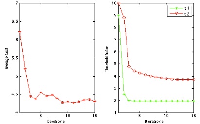
Figure 4: Sample cost and parameter trajectories for $1/\bar{\alpha}=[2,6]$, $\theta=[10,30,10,30]$, and $s_{0}=[9,10]$

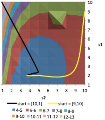
Figure 5: Cost surface and convergence trajectories for Scenario A (note: the color scale refers to the cost values)

In our second set of simulations, we perform a sequential optimization of the cycle lengths and threshold values. We make use of the optimal light cycle lengths obtained through IPA (denoted by $\mathbf{\theta}_{IPA}^{\ast}=\left[\theta_{1,\min}^{\ast},\theta_{1,\max}^{\ast},\theta_{2,\min}^{\ast},\theta_{2,\max}^{\ast}\right]$) by Geng and Cassandras (2013b), and subsequently apply the IPA estimator derived in this paper to optimize the queue content thresholds. The optimal light cycle lengths obtained by Geng and Cassandras (2013b) for fixed and predetermined threshold values of $\mathbf{s}=\left[8,8\right]$ were $\mathbf{\theta}_{IPA}^{\ast}=\left[10.2,19.3,10.1,16.3\right]$ for $1/\overline{\alpha}=[2,3]$ and $\mathbf{\theta}_{IPA}^{\ast}=\left[10.1,20.1,10.6,11.9\right]$ for $1/\overline{\alpha}=[1.7,3]$. A comparison between IPA and BF results, including a quantitative assessment of the additional cost reduction achieved (computed as a percentage of the initial cost and labeled $R$) is shown in Table 2.

Table 2: Optimization results for system with optimal cycle lengths

	IPA			BF
$1/\overline{\alpha}$	$s_{IPA}^{\ast}$	$J_{IPA}^{\ast}$	$R$ $(\%)$	$s_{BF}^{\ast}$	$J_{BF}^{\ast}$
$\left[2,3\right]$	$\left[2.8,4.3\right]$	$7.1$	$15$	$\left[2,5\right]$	$7.2$
$\left[1.7,3\right]$	$\left[4.8,6.1\right]$	$14.9$	$11$	$\left[3,8\right]$	$15.7$

In order to further illustrate the advantage of quasi-dynamically controlling the light cycle lengths and threshold values over a static IPA approach to the TLC problem, we include a comparison of the results generated by our methodology with those obtained when static control (as described by Geng and Cassandras (2012)) is applied to determine the optimal cycle lengths $\mathbf{\theta}_{static}^{\ast}$. The static controller defined by Geng and Cassandras (2012) adjusts the green light cycles subject to some lower and upper bounds and determines $\mathbf{\theta}_{static}^{\ast}=\left[\theta_{1}^{\ast},\theta_{2}^{\ast}\right]$, where $\theta_{1}^{\ast}$ ($\theta_{2}^{\ast}$, respectively) is the green cycle length which should be allotted to road $1$ (road $2$, respectively) in order to minimize the average queue content on both roads. Table 3 summarizes the results obtained by each of the IPA approaches considered in this work: Method 1, in which a static controller is used to adjust the light cycles (results were obtained by using the same setting as in our second set of quasi-dynamic simulations and constraining $\theta\in\left[10,40\right]$); Method 2, in which only the light cycles are controlled quasi-dynamically (i.e. fixed and predetermined queue content thresholds are incorporated into the system model); Method 3, in which a sequential quasi-dynamic optimization of light cycle lengths and threshold values is performed in between two adjustment points. The columns labeled $R_{i}$, $i=2,3$, present the cost reduction achieved by the quasi-dynamic methods with respect to the static approach, i.e. $R_{i}=\frac{J_{1}^{\ast}-J_{i}^{\ast}}{J_{1}^{\ast}}\ast 100$.

Table 3: Comparison between three IPA-based approaches to the TLC problem

	Method 1	Method 2		Method 3
$1/\overline{\alpha}$	$J_{1}^{\ast}$	$J_{2}^{\ast}$	$R_{2}$ $(\%)$	$J_{3}^{\ast}$	$R_{3}$ $(\%)$
$\left[2,3\right]$	$14.4$	$8.4$	$42$	$7.1$	$51$
$\left[1.7,3\right]$	$23.9$	$16.7$	$30$	$14.9$	$38$

5 Conclusion

We have modeled a single traffic light intersection as an SFM and formulated the corresponding TLC problem within a quasi-dynamic control setting to which IPA techniques were applied in order to derive gradient estimates of a cost metric with respect to controllable queue content threshold values. By subsequently incorporating these estimators into a gradient-based optimization algorithm, numerical results were obtained which substantiate our claims that: $(i)$ a considerable reduction in the mean queue content of both roads can be achieved by quasi-dynamically controlling the thresholds in systems with non-optimal cycle lengths; $(ii)$ determining optimal threshold values allows for additional improvements to the performance of systems running under optimal cycle lengths. Such results lead us to believe that a method in which the light cycle lengths and queue content thresholds are controlled simultaneously is likely to provide improved solutions to the TLC problem. Our ongoing research is, therefore, focused on deriving an IPA-based optimization algorithm that incorporates all such controllable parameters and ultimately determines the optimal light cycle length/threshold configuration capable of minimizing traffic build-up at a given traffic light intersection. Future work includes applying IPA to an intersection with more complicated traffic flow (e.g. allowing for left- and right-turns), incorporating acceleration/deceleration due to light switches into the flow model, as well as extending our methodology to multiple intersections.

References

- Alvarez and Poznyak (2010) Alvarez, I., Poznyak, A. (2010). Game Theory Applied to Urban Traffic Control Problem. Proceedings of the International Conference on Control, Automation and Systems, 2164-2169.
- Cassandras and Lafortune (2008) Cassandras, C.G., Lafortune, S. (2008). Introduction to Discrete Event Systems. Springer, New York, 2nd edition.
- Cassandras and Lygeros (2006) Cassandras, C.G., Lygeros, J. (2006). Stochastic Hybrid Systems. Taylor and Francis, Boca Raton.
- Cassandras et al. (2002) Cassandras, C.G., Wardi, Y., Melamed, B., Sun, G., and Panayiotou, C.G. (2002). Perturbation analysis for on-line control and optimization of stochastic fluid models. IEEE Trans. Automat. Control, 47, 1234-1248.
- Cassandras et al. (2010) Cassandras, C.G., Wardi, Y., Panayiotou, C.G., and Yao, C. (2010). Perturbation analysis and optimization of stochastic hybrid systems. European Journal of Control, 16, 642-664.
- Choi et al. (2002) Choi, W., Yoon, H., Kim, K., Chung, I., and Lee, S. (2002). A Traffic Light Controlling FLC Considering the Traffic Congestion. Proceedings of the AFSS 2002 International Conference on Fuzzy Systems, 69-75.
- De Schutter (1999) De Schutter, B. (1999). Optimal Traffic Light Control for a Single Intersection. Proceedings of the American Control Conference, 2195-2199.
- Dujardin et al. (2011) Dujardin, Y., Boillot, F., Vanderpooten, D., and Vinant, P. (2011). Multiobjective and multimodal adaptive traffic light control on single junctions. Proceedings of the IEEE Conference on Intelligent Transportation Systems, 1361-1368.
- Fu and Howell (2003) Fu, M.C., Howell, W.C. (2003). Application of Perturbation Analysis to Traffic Light Signal Timing. Proceedings of the IEEE Conference on Decision and Control, 4837-4840.
- Geng and Cassandras (2012) Geng, Y., Cassandras, C.G. (2012). Traffic Light Control Using Infinitesimal Perturbation Analysis. Proceedings of the IEEE Conference on Decision and Control, 7001-7006.
- Geng and Cassandras (2013a) Geng, Y., Cassandras, C.G. (2013a). Multi-intersection Traffic Light Control with blocking. Preprint at http://link.springer.com/article/10.1007/s10626-013-0176-0#page-1.
- Geng and Cassandras (2013b) Geng, Y., Cassandras, C.G. (2013b). Quasi-dynamic Traffic Light Control for a Single Intersection. Proceedings of the 52nd IEEE Conference on Decision and Control.
- Head et al. (1996) Head, L., Ciarallo, F., and Kaduwella, D.L. (1996). A perturbation analysis approach to traffic signal optimization. INFORMS National Meeting.
- Panayiotou et al. (2005) Panayiotou, C.G., Howell, W.C., and Fu, M. (2005). Online Traffic Light Control through Gradient Estimation using Stochastic Fluid Models. Proceedings of the IFAC World Congress.
- Porche et al. (1996) Porche, I., Sampath, M., Sengupta, R., Chen. Y.-L., and Lafortune, S. (1996). A Decentralized Scheme for Real-Time Optimization of Traffic Signals. Proceedings of the IEEE International Conference on Control Applications, 582-589.
- Wardi et al. (2010) Wardi, Y., Adams, R., and Melamed, B. (2010). A unified approach to infinitesimal perturbation analysis in stochastic flow models: the single-stage case. IEEE Trans. Automat. Control, 55, 89-103.
- Yao and Cassandras (2011) Yao, C., Cassandras, C.G. (2011). Perturbation analysis of stochastic hybrid systems and applications to resource contention games. Frontiers of Electrical and Electronic Engineering in China, 6, 453-467.
- Yu and Recker (2006) Yu, X.-H., Recker, W.W. (2006). Stochastic adaptive control model for traffic light systems. Transportation Research Part C: Emerging Technology, 14, 263-282.
- Zhao and Chen (2003) Zhao, X., Chen, Y. (2003). Traffic Light Control Method for a Single Intersection Based on Hybrid Systems. Proceedings of the IEEE Conference on Intelligent Transportation Systems, 1105-1109.