Testing non-nested structural equation models

Abstract

In this paper, we apply Vuong’s (1989) likelihood ratio tests of non-nested models to the comparison of non-nested structural equation models. Similar tests have been previously applied in SEM contexts (especially to mixture models), though the non-standard output required to conduct the tests has limited their previous use and study. We review the theory underlying the tests and show how they can be used to construct interval estimates for differences in non-nested information criteria. Through both simulation and application, we then study the tests’ performance in non-mixture SEMs and describe their general implementation via free R packages. The tests offer researchers a useful tool for non-nested SEM comparison, with barriers to test implementation now removed.

This work was supported by National Science Foundation grant SES-1061334. Portions of the work were presented at the 2014 Meeting of the Psychometric Society and at the 2015 International Workshop on Psychometric Computing (Psychoco 2015). We thank Achim Zeileis and three anonymous reviewers for comments that improved the paper. All remaining errors are solely the responsibility of the authors. Correspondence to Edgar C. Merkle, Department of Psychological Sciences, University of Missouri, Columbia, MO 65211. Email: merklee@missouri.edu.

Researchers frequently rely on model comparisons to test competing theories. This is especially true when structural equation models (SEMs) are used, because the models are often able to accommodate a large variety of theories. When competing theories can be translated into nested SEMs, the comparison is relatively easy: one can compute likelihood ratio statistics using the results of the fitted models [<]e.g.,>stesha85. The test associated with this likelihood ratio statistic yields one of two conclusions: the two models fit equally well, so that the simpler model is to be preferred, or the more complex model fits better, so that it is to be preferred. As is well known, however, the likelihood ratio statistic does not immediately extend to situations where models are non-nested.

In the non-nested case, researchers typically rely on information criteria for model comparison, including the Akaike Information Criterion [<]AIC;>aka74 and the Bayesian Information Criterion [<]BIC;>sch78. One computes an AIC or BIC for the two models, then selects the model with the lowest criterion as “best.” Thus, the applied conclusion differs slightly from the likelihood ratio test (LRT): we conclude from the information criteria that one or the other model is better, while we conclude from the LRT either that the complex model is better or that there is insufficient evidence to differentiate between model fits.

While information criteria can be applied to non-nested models, the popular “select the model with the lowest” decision criterion can be problematic. In particular, premer12 showed that BIC exhibits large variability at the sample sizes typically used in SEM contexts. Thus, the model that is preferred for a given sample often will not be preferred in new samples. Preacher and Merkle studied a series of nonparametric bootstrap procedures to estimate sampling variability in BIC, but no procedure succeeded in fully characterizing this variability.

A problem with the “select the model with the lowest” decision criterion involves the fact that one can never conclude that the models fit equally. There may often be situations where the models exhibit “close” values of the information criteria, yet one of the models is still selected as best. To handle this issue, porwu13 developed a parametric bootstrap method that allows one to conclude that the two models are equally good (in addition to concluding that one or the other model fits better). Their results indicated that the procedure is promising, though it is also computationally expensive: one must draw a large number of bootstrap samples from each of the two fitted models, then refit each model to each bootstrap sample.

In this paper, we study formal tests of non-nested models that allow us to conclude that one model fits better than the other, that the two models exhibit equal fit, or that the two models are indistinguishable in the population of interest. The tests are based on the theory of Vuong vuo89, and one of the tests is popularly applied to the comparison of mixture models with different numbers of components <including count regression models and factor mixture models;>gre94,lomen01,nylmut07. While some authors have recently described problems with mixture model applications jef03; wil15, the tests have the potential to be very useful in general SEM contexts. This is because non-nested SEMs are commonly observed throughout psychology <e.g.,>fregar07,kim02,santod02.

levhan07,levhan11 have previously studied the application of Vuong’s vuo89 theory to structural equation models, describing relevant background and proposing steps by which researchers can carry out tests of non-nested models. Levy and Hancock bypass an important step of the theory due to the non-standard model output required, instead requiring researchers to algebraically examine the candidate models and to potentially carry out likelihood ratio tests between each candidate model and a constrained version of the models. This procedure can accomplish the desired goal, but it also requires a considerable amount of analytic and computational work on the part of the user. We instead study the tests as Vuong originally proposed them, using the non-standard model output that is required. This study is aided by our general implementation of the tests, available via the R package nonnest2 nonnest2.

In the following pages, we first describe the relevant theoretical results from Vuong vuo89. We also show how the theory can be used to obtain confidence intervals for differences in BICs (and other information criteria) associated with non-nested models. Next, we apply the tests to data on teacher burnout, which were originally examined by Byrne byrne1994burnout. Next, we describe the results of three simulations that illustrate test properties in the context of SEM. Finally, we discuss recommendations, extensions, and practical issues.

1 Theoretical Background

In this section, we provide an overview of the theory underlying the test statistics. The overview is largely based on Vuong vuo89, and the reader is referred to that paper for further detail. For alternative overviews of the theory, see gol00 and levhan07. The theory is applicable to many models estimated via Maximum Likelihood (ML), though we focus on structural equation models here.

We consider situations where two candidate structural equation models, $M_{A}$ and $M_{B}$, are to be compared using a dataset $\bm{X}$ with $n$ cases and $p$ manifest variables. $M_{A}$ may be represented by the equations

$$\bm{x}_{i} =\bm{\nu}_{A}+\bm{\Lambda}_{A}\bm{\eta}_{A,i}+\bm{\epsilon}_{A,i}$$ (1)

$$\bm{\eta}_{A,i} =\bm{\alpha}_{A}+\bm{B}_{A}\bm{\eta}_{A,i}+\bm{\zeta}_{A,i},$$ (2)

where $\bm{\eta}_{A,i}$ is a vector containing the latent variables in $M_{A}$; $\bm{\epsilon}_{A,i}$ and $\bm{\zeta}_{A,i}$ are zero-centered residual vectors, independent across values of $i$; $\bm{\Lambda}_{A}$ is a matrix of factor loadings; and $\bm{B}_{A}$ contains parameters that reflect directed paths between latent variables. The second model, $M_{B}$, is defined similarly, and we restrict ourselves to situations where the residuals and latent variables are assumed to follow multivariate normal distributions (though this distributional assumption is not required to use the test statistics; see the General Discussion).

The $M_{A}$ parameter vector, $\bm{\theta}_{A}$, includes the parameters in $\bm{\nu}_{A}$, $\bm{\Lambda}_{A}$, $\bm{\alpha}_{A}$, and $\bm{B}_{A}$, along with variance and covariance parameters related to the latent variables and residuals. These parameters imply a marginal multivariate normal distribution for $\bm{x}_{i}$ with a specific mean vector (typically $\bm{\nu}_{A}$) and covariance matrix <see, e.g.,>broarm95, which allows us to estimate the model via ML. In particular, we will choose $\hat{\bm{\theta}}_{A}$ to maximize the log-likelihood ($\ell()$):

$$\ell(\bm{\theta}_{A};\bm{x}_{1},\dots,\bm{x}_{n})\leavevmode\nobreak\ =\leavevmode\nobreak\ \sum_{i=1}^{n}\ell(\bm{\theta}_{A};\bm{x}_{i})\leavevmode\nobreak\ =\leavevmode\nobreak\ \sum_{i=1}^{n}\log f_{A}(\bm{x}_{i};\bm{\theta}_{A}),$$

where $f_{A}(\bm{x}_{i};\bm{\theta}_{A})$ is the probability density function (pdf) of the multivariate normal distribution, with mean vector and covariance matrix implied by $M_{A}$ and its parameter vector $\bm{\theta}_{A}$. Similarly, the parameters $\hat{\bm{\theta}}_{B}$ are chosen to maximize the log-likelihood $\ell(\bm{\theta}_{B};\bm{x}_{1},\dots,\bm{x}_{n})$.

Instead of defining the ML estimates as above, we could equivalently define them via the gradients

$$s(\hat{\bm{\theta}}_{A};\bm{x}_{1},\dots,\bm{x}_{n})=\sum_{i=1}^{n}{\bm{s}}(\hat{\bm{\theta}}_{A};\bm{x}_{i}) \leavevmode\nobreak\ =\leavevmode\nobreak\ 0$$

$$s(\hat{\bm{\theta}}_{B};\bm{x}_{1},\dots,\bm{x}_{n})=\sum_{i=1}^{n}{\bm{s}}(\hat{\bm{\theta}}_{B};\bm{x}_{i}) \leavevmode\nobreak\ =\leavevmode\nobreak\ 0,$$

where the gradients sum scores across individuals (where scores are defined as the casewise contributions to the gradient). The above equations simply state that we choose parameters such that the gradient (first derivative of the likelihood function) equals zero. Assuming that $M_{A}$ has $k$ free parameters, the associated score function may be explicitly defined as

$${\bm{s}}({\bm{\theta}}_{A};\bm{x}_{i})\leavevmode\nobreak\ =\leavevmode\nobreak\ \left(\frac{\partial\ell({\bm{\theta}}_{A};\bm{x}_{i})}{\partial\theta_{A,1}},\dots,\frac{\partial\ell({\bm{\theta}}_{A};\bm{x}_{i})}{\partial\theta_{A,k}}\right)^{\prime},$$ (3)

with the score function for $M_{B}$ defined similarly (where the number of free parameters for $M_{B}$ is $q$ instead of $k$). We also define $M_{A}$’s expected information matrix as

$$\bm{\mathrm{I}}(\bm{\theta}_{A})=-\mathrm{E}\ \frac{\partial^{2}\ell({\bm{\theta}}_{A};\bm{x}_{1},\ldots,\bm{x}_{n})}{\partial\bm{\theta}_{A}\partial\bm{\theta}_{A}^{\prime}}$$ (4)

where, again, the information matrix of $M_{B}$ is defined similarly.

Figure 1: Path diagram reflecting the models used in the simulation. Model A is the data-generating model, with the loading labeled ‘A’ varying across conditions.

The statistics described here can be used in general model comparison situations, where one is interested in which of two candidate models ($M_{A}$ and $M_{B}$) is closest to the data-generating model in Kullback–Leibler distance kullei51. Letting $g()$ be the density of the data-generating model (which is generally unknown), the distances for $M_{A}$ and $M_{B}$ can be denoted $\text{KL}_{Ag}$ and $\text{KL}_{Bg}$, respectively. The distance $\text{KL}_{Ag}$ may be explicitly written as

$$\text{KL}_{Ag} =\displaystyle\int\log\left(\frac{g(\bm{x})}{f_{A}(\bm{x};\bm{\theta}^{*}_{A})}\right)g(\bm{x})d\bm{x}$$ (5)

$$=\mathrm{E}\left[\log(g(\bm{x}))\right]-\mathrm{E}\left[\log(f_{A}(\bm{x};\bm{\theta}^{*}_{A}))\right],$$ (6)

where $\bm{\theta}^{*}_{A}$ is the $M_{A}$ parameter vector that minimizes this distance (also called the “pseudo-true” parameter vector) and where the expected values are taken with respect to $g()$. The “pseudo-true” name arises from the fact that $\bm{\theta}^{*}_{A}$ usually does not reflect the true parameter vector (because the candidate model $M_{A}$ is usually incorrect). However, the parameter vector is pseudo-true in the sense that it allows $M_{A}$ to most closely approximate the truth.

1.1 Relationships Between Models

Relationships between pairs of candidate models may be characterized in multiple manners. Familiarly, nested models are those for which the parameter space associated with one model is a subset of the parameter space associated with the other model; every set of parameters from the less-complex model can be translated into an equivalent set of parameters from the more-complex model. Similarly, non-nested models are those whose parameter spaces each include some unique points. Aside from these two broad, familiar classifications, however, we may define other relationships between models. These include the concepts of equivalence, overlappingness, and strict non-nesting. The latter two concepts refer to specific types of non-nested models. All three are described below.

Many SEM researchers are familiar with the concept of model equivalence <e.g.,>hermar13,leeher90,macweg93: two seemingly-different SEMs yield exactly the same implied moments (mean vectors and covariance matrices) and fit statistics when fit to any dataset. SEM researchers are less familiar with the concept of overlapping models: these are models that yield exactly the same implied moments and fit statistics for some populations but not for others. Further, even if the models yield identical moments in our population of interest, they will be exactly identical only in the population. Fits to sample data will generally yield different moments and fit statistics.

An example of overlapping models is displayed in Figure 1. Both $M_{A}$ and $M_{B}$ are two-factor models, where $M_{A}$ has a free path from $\eta_{1}$ to $X_{4}$ and $M_{B}$ has a free path from $\eta_{2}$ to $X_{3}$. These models are overlapping: their predictions and fit statistics will usually differ, but they will be the same in populations where the parameters labeled ‘A’ and ‘B’ both equal zero. Even if these two paths equal zero in the population, they generally will not equal zero when the models are fit to sample data. Therefore, the models will not have the same implied moments and fit statistics when fit to sample data. This means that, given sample data, we must test whether or not the models are distinguishable in the population of interest. Note that overlappingness is a general relationship between two models regardless of the focal population, whereas distinguishability is a specific relationship between models in the context of a single focal population.

Overlapping models are one sub-classification of non-nested models. The other sub-classification is strictly non-nested models; these are models whose parameter spaces do not overlap at all. In other words, strictly non-nested models never yield the same implied moments and fit statistics for any population. Strictly non-nested models may have different functional forms (say, an exponential growth model versus a logistic growth model) or may make different distributional assumptions.

It is often difficult to know whether or not candidate SEMs are overlapping. Consider the path models in Figure 2, which reflect four potential hypotheses about the relationships between nine observed variables. These models are obviously non-nested, but are they overlapping or strictly non-nested? Assuming that all models employ the same data distribution (typically multivariate normal), then the models will be indistinguishable in populations where all observed variables are independent of one another. Therefore, SEMs that employ the same form of data distribution will typically be overlapping. In other situations, it may be difficult to tell whether or not the candidate models are overlapping. Thus, it is important to test for distinguishability when doing model comparisons: if the observed data imply that the models are indistinguishable in the population of interest, then there is no point in further model comparison. This is especially relevant to the use of information criteria for non-nested model comparison, where one is guaranteed to select a candidate model as better (at least, using the standard decision criteria). Additionally, as we will see below, when a pair of models is non-nested, the limiting distribution of the likelihood ratio statistic depends on whether or not the models are distinguishable.

Figure 2: Path diagrams reflecting the models used in Simulation 2.

Model A ($df=27$)

Model B ($df=21$)

Model C ($df=20$)

Model D ($df=26$)

The above discussion suggests a sequence of tests for comparing two models. Assuming that the models are not equivalent to one another (regardless of population), we must establish that the models are distinguishable in the population of interest. Assuming that the models are distinguishable, we can then compare the models’ fits and potentially select one as better. Below, we describe test statistics that can be used in this sequence.

1.2 Test Statistics

Vuong’s vuo89 tests of distinguishability and of model fit utilize the terms $\ell(\hat{\bm{\theta}}_{A};\bm{x}_{i})$ and $\ell(\hat{\bm{\theta}}_{B};\bm{x}_{i})$ for $i=1,\ldots,n$, which are the casewise likelihoods evaluated at the ML estimates. For the purpose of SEM, we focus on two separate statistics that Vuong proposed. One statistic tests whether or not models are distinguishable, and the other tests the fit of non-nested, distinguishable models. These tests proceed sequentially in situations where we are unsure whether or not the two models are distinguishable in the population of interest. If we know in advance that two models are not overlapping, we can proceed directly to the second test.

To gain an intuitive feel for the tests, imagine that we fit both $M_{A}$ and $M_{B}$ to a data set and then obtain $\ell(\hat{\bm{\theta}}_{A};\bm{x}_{i})$ and $\ell(\hat{\bm{\theta}}_{B};\bm{x}_{i})$ for $i=1,\ldots,n$. To test whether or not the models are distinguishable, we can calculate a likelihood ratio for each case $i$ and examine the variability in these $n$ ratios. If the models are indistinguishable, then these ratios should be similar for all individuals, so that their variability is close to zero. If the models are distinguishable, then the variability in the casewise likelihood ratios characterizes general sampling variability in the likelihood ratio between $M_{A}$ and $M_{B}$, allowing for a formal model comparison test that does not require the models to be nested.

To formalize the ideas in the previous paragraph, we characterize the population variance in individual likelihood ratios of $M_{A}$ vs $M_{B}$ as

$$\omega^{2}_{*}=\text{var}\left[\log\frac{f_{A}(\bm{x}_{i};\bm{\theta}^{*}_{A})}{f_{B}(\bm{x}_{i};\bm{\theta}^{*}_{B})}\right]\ \ i=1,\ldots,n,$$

where this variance is taken with respect to the pseudo-true parameter vectors introduced in Equation (5). This means that we make no assumptions that either candidate model is the true model. Using the above equation, hypotheses for a test of model distinguishability may then be written as

$$H_{0}\colon \ \omega^{2}_{*}=0$$ (7)

$$H_{1}\colon \ \omega^{2}_{*}>0,$$ (8)

with a sample estimate of $\omega^{2}_{*}$ being

$$\hat{\omega}^{2}_{*}=\frac{1}{n}\displaystyle\sum_{i=1}^{n}\left[\log\frac{f_{A}(\bm{x}_{i};\hat{\bm{\theta}}_{A})}{f_{B}(\bm{x}_{i};\hat{\bm{\theta}}_{B})}\right]^{2}-\left[\frac{1}{n}\displaystyle\sum_{i=1}^{n}\log\frac{f_{A}(\bm{x}_{i};\hat{\bm{\theta}}_{A})}{f_{B}(\bm{x}_{i};\hat{\bm{\theta}}_{B})}\right]^{2}.$$ (9)

Division by $(n-1)$ instead of $n$ is also possible to reduce bias in the estimate, though this will have little impact at the sample sizes typically observed in SEM applications.

Vuong shows that, under (7) and mild regularity conditions (ensuring that second derivatives of the likelihood function exist, observations are i.i.d., and the ML estimates are unique and not on the boundary), $n\hat{\omega}^{2}_{*}$ is asymptotically distributed as a particular weighted sum of $\chi^{2}$ distributions. Weighted sums of $\chi^{2}$ distributions arise when we sum the squares of normally-distributed variables; the normally-distributed variables involved in the test statistics here are the ML estimates $\hat{\bm{\theta}}_{A}$ and $\hat{\bm{\theta}}_{B}$. The weights involved in this sum are obtained via the squared eigenvalues of a matrix $\bm{W}$ that arises from the candidate models’ scores (Equation (3)) and information matrices (Equation (4)); see the Appendix for details. This result immediately allows us to test (7) using results from the two fitted models. If the null hypothesis is not rejected, we conclude that the models cannot be distinguished in the population of interest. In the case where models are nested, this conclusion would lead us to prefer the model with fewer degrees of freedom. In the case where models are not nested, the two candidate models may have the same degrees of freedom. Thus, depending on the specific models being compared, we might not prefer either model.

The software requirements for carrying out the test of (7) is somewhat non-standard. For each candidate model, we need to obtain the scores from (3) and information matrix from (4). We then need to arrange this output in matrices, do some multiplications to obtain a new matrix, and obtain eigenvalues of this new matrix. Further, we need the ability to evaluate quantiles of weighted sum of $\chi^{2}$ distributions. The difficulty in obtaining these results led levhan07 to bypass the test of model distinguishability and instead conduct an algebraic model comparison that provides evidence about whether or not the models are distinguishable. Whereas this algebraic comparison is reasonable, it does not always indicate whether or not models are distinguishable. Further, it is more complicated for the applied researcher who wishes to use these tests (assuming that an implementation of the statistical test is available).

Assuming that the null hypothesis from (7) is rejected (i.e., that the models are distinguishable), we may compare the models via a non-nested LRT. We can write the hypotheses associated with this test as

$$H_{0}\colon \ \mathrm{E}[\ell(\hat{\bm{\theta}}_{A};\bm{x}_{i})]=\mathrm{E}[\ell(\hat{\bm{\theta}}_{B};\bm{x}_{i})]$$ (10)

$$H_{1A}\colon \ \mathrm{E}[\ell(\hat{\bm{\theta}}_{A};\bm{x}_{i})]>\mathrm{E}[\ell(\hat{\bm{\theta}}_{B};\bm{x}_{i})]$$ (11)

$$H_{1B}\colon \ \mathrm{E}[\ell(\hat{\bm{\theta}}_{A};\bm{x}_{i})]<\mathrm{E}[\ell(\hat{\bm{\theta}}_{B};\bm{x}_{i})],$$ (12)

where the expectations arise from the K-L distance in Equation (6) (note that we don’t need to consider the expected value of $\log(g(\bm{x}))$ because it is constant across candidate models). The hypothesis $H_{0}$ above states that the K-L distance between $M_{A}$ and the truth equals the K-L distance between $M_{B}$ and the truth; this is like stating that the two models have equal population discrepancies. The test is written to be directional, so that one chooses either $H_{1A}$ or $H_{1B}$ prior to carrying out the test. In practice, however, a two-tailed test is often carried out, with a single model being preferred in the situation where $H_{0}$ is rejected. This follows the framework of jontuk01, whereby there are three possible conclusions available to researchers: $M_{A}$ is closer to the truth (in K-L distance) than $M_{B}$; $M_{B}$ is closer to the truth than $M_{A}$; or there is insufficient evidence to conclude that either model is closer to the truth than the other.

For non-nested, distinguishable models, Vuong shows that

$$\text{LR}_{AB}=n^{-1/2}\displaystyle\sum_{i=1}^{n}\log\frac{f_{A}(\bm{x}_{i};\hat{\bm{\theta}}_{A})}{f_{B}(\bm{x}_{i};\hat{\bm{\theta}}_{B})}\leavevmode\nobreak\ \overset{d}{\rightarrow}\leavevmode\nobreak\ N(0,\omega^{2}_{*})$$ (13)

under (10) and the regularity conditions noted above. Thus, we obtain critical values and $p$-values by comparing the non-nested LRT statistic to the standard normal distribution. Assuming that the desired Type I error rate is $\alpha_{2}$ for this test and that the desired Type I error rate is $\alpha_{1}$ for the test of (7), Vuong shows that the sequence of tests has an overall Type I error rate that is bounded from above by $\text{max}(\alpha_{1},\alpha_{2})$. In practical applications, it is customary to set $\alpha_{1}=\alpha_{2}$.

Assuming that the null hypothesis from (7) is not rejected (i.e., that the models are indistinguishable), Vuong shows that $2n^{1/2}\text{LR}_{AB}$ follows a weighted sum of $\chi^{2}$ distributions, where the weights are obtained from the unsquared eigenvalues of the same matrix $\bm{W}$ that arose in the test of (7). This result is not typically used in the case of non-nested models: we first need the test of $\omega^{2}_{*}$ to determine the limiting distribution that we should use for the likelihood ratio (either the normal distribution from (13) or the weighted sum of $\chi^{2}$ distribution described here). If the test of $\omega^{2}_{*}$ indicates indistinguishable models, however, then there is no point in further testing the models via $2n^{1/2}\text{LR}_{AB}$. If the test of $\omega^{2}_{*}$ indicates distinguishable models, then we rely on the limiting distribution from (13) instead of the weighted sum of $\chi^{2}$s. The result described in this paragraph can be used to compare nested models, however, and we return to this topic in the next subsection.

The test statistics described above are implemented for general multivariate normal SEMs (and other models) in the free R package nonnest2 nonnest2. Models are first estimated via lavaan lavaan11, then nonnest2 computes the test statistics based on the fitted models’ output. In the following sections, we describe ways in which these ideas can be extended to test nested models and to test information criteria.

1.3 Testing Nested Models

In the situation where $M_{B}$ is nested within $M_{A}$, the likelihood ratio and the variance statistic $n\omega_{*}^{2}$ can each be used to construct a unique test of $M_{A}$ versus $M_{B}$. For nested models, the null hypotheses (7) and (10) can be shown to be the same as the traditional null hypothesis:

$$H_{0}\colon \ \bm{\theta}_{A}\in\ h(\bm{\theta}_{B})$$ (14)

$$H_{1}\colon \ \bm{\theta}_{A}\not\in\ h(\bm{\theta}_{B}),$$ (15)

where $h()$ is a function translating the $M_{B}$ parameter vector to an equivalent $M_{A}$ parameter vector. In the general case, where $M_{A}$ is not assumed to be correctly specified, the statistics $n\hat{\omega}^{2}_{*}$ and $2n^{1/2}\text{LR}_{AB}$ (see Equations (9) and (13)) both strongly converge <i.e., almost surely;>casber02 to weighted sums of $\chi^{2}$ distributions under the null hypothesis from (14). The specific weights differ between the two statistics; the weights associated with $n\hat{\omega}^{2}_{*}$ are the squared eigenvalues of a $\bm{W}$ matrix that is defined in the Appendix, whereas the weights associated with $2n^{1/2}\text{LR}_{AB}$ are the unsquared eigenvalues of the same $\bm{W}$ matrix. This result differs from the usual multivariate normal SEM derivations <e.g.,>ameand90,stesha85, which employ either an assumption that $M_{A}$ is correctly specified or that the population parameters drift toward a point that is contained in $M_{A}$’s parameter space <see>[for further discussion of this point and fit assessment of single models]chusha09. Under the assumption that $M_{A}$ is correctly specified, the statistics $n\hat{\omega}^{2}_{*}$ and $2n^{1/2}\text{LR}_{AB}$ weakly converge (i.e., in distribution) to the usual $\chi^{2}_{\text{df}=q-k}$ distribution under (14). Hence, the framework here provides a more general characterization of the nested LRT than do traditional derivations.

1.4 Testing Information Criteria

Model selection with AIC or BIC (i.e., selecting the model with the lowest) involves adjustment of the likelihood ratio by a constant term that penalizes the two models for complexity. Thus, as Vuong vuo89 originally described, the above results can be extended to test differences in AIC or BIC. To show this formally, we focus on BIC and write the BIC difference between two models as:

$$\text{BIC}_{A}-\text{BIC}_{B}=(k\log n-q\log n)-2\displaystyle\sum_{i=1}^{n}\log\frac{f_{A}(\bm{x}_{i};\hat{\bm{\theta}}_{A})}{f_{B}(\bm{x}_{i};\hat{\bm{\theta}}_{B})},$$

where $k$ and $q$ are the number of free parameters for $M_{A}$ and $M_{B}$, respectively. This shows that we are simply taking a linear transformation of the usual likelihood ratio, so that the test of (7) and the result from (13) apply here. In particular, if models are indistinguishable, then one could select the model that BIC penalizes the least (i.e., the model with fewer parameters). If models are distinguishable, then we may formulate a hypothesis that $\text{BIC}_{A}=\text{BIC}_{B}$. Under this hypothesis, the result from (13) can be used to show that

$$n^{-1/2}\left[((k-q)\log n)-2\displaystyle\sum_{i=1}^{n}\log\frac{f_{A}(\bm{x}_{i};\hat{\bm{\theta}}_{A})}{f_{B}(\bm{x}_{i};\hat{\bm{\theta}}_{B})}\right]\leavevmode\nobreak\ \overset{d}{\rightarrow}\leavevmode\nobreak\ N(0,4\omega^{2}_{*}).$$

This result can be used to obtain an “adjusted” test statistic that accounts for the models’ relative complexity. Alternatively, we prefer to use this result to construct a $100\times(1-\alpha)$% confidence interval associated with the BIC difference. This is obtained via

$$(\text{BIC}_{A}-\text{BIC}_{B})\pm z_{1-\alpha/2}\sqrt{4n\omega^{2}_{*}},$$ (16)

where $z_{1-\alpha/2}$ is the variate at which the cumulative distribution function (cdf) of the standard normal distribution equals $(1-\alpha/2)$. To coincide with the tests described previously, $\alpha$ should be the same as the $\alpha$ level used for the test of distinguishability.

To our knowledge, this is the first analytic confidence interval for a non-nested difference in information criteria that has been presented in the SEM literature. This confidence interval is simpler to calculate than bootstrap intervals <see, e.g.,>[for a discussion of bootstrap procedures]premer12, and, as shown later, its coverage is often comparable. The bootstrap intervals may still be advantageous if regularity conditions are violated.

1.5 Relation to the Nesting and Equivalence Test

bentler2010testing describe a Nesting and Equivalence Test (NET) that assesses whether two models provide exactly the same fit to sample data, relying on the fact that equivalent models can perfectly fit one another’s implied mean vectors and covariance matrices. As previously described, this differs from the “indistinguishability” characteristic that is relevant to the tests in this paper. Indistinguishable models provide exactly the same fit in the population but not necessarily to sample data.

The NET procedure is convenient and computationally simple, and it is generally suited to examining whether two models are globally nested or equivalent across large sets of covariance matrices <though see>[for some pathological cases]bentler2010testing. It cannot, however, inform us about whether or not two models are distinguishable based on the sample data. In other words, equivalent models are indistinguishable, but indistinguishable models are not necessarily equivalent. Thus, the two methods are complementary: we can use the NET to determine whether two models can possibly be distinguished from each another, while we can use the test of (7) to determine whether two models can be distinguished in the population of interest. In the following sections, we study the tests’ applications to SEM using both simulation and real data.

2 Application: Teacher Burnout

2.1 Background

byrne1994burnout tested the impact of organizational and personality variables on three dimensions of teacher burnout. The application here is limited to the sample of elementary teachers only ($n=599$; intermediate and secondary school teachers were also observed) and utilizes models that are related to those presented in Chapter 6 of byrne2009structural.

Figure 3: Path diagram of candidate Models 1, 2, and 3, which are related to those originally specified by Byrne (2009). Only latent variables are displayed, and covariances between exogenous variables are always estimated.

2.2 Method

The candidate models that we consider are illustrated in Figure 3, which shows only the latent variables included in the model (and not the indicators of the latent variables or variance parameters). The figure displays candidate model $M_{1}$, with dotted lines reflecting parameters that are added or removed in models $M_{2}$ and $M_{3}$. Each pair of models is non-nested, so BIC (or some other information criterion) would typically be used to select a model from the set. Alternatively, we can use the statistics described in this paper to study the models’ distinguishability and fit in greater detail.

To expand on the model comparison procedure, we first use the NET bentler2010testing to determine whether or not pairs of models are equivalent to one another. For models that are not equivalent, we then use Vuong’s distinguishability test to make inferences about whether or not each pair of models is distinguishable based on the focal population of elementary teachers. Finally, we use Vuong’s non-nested LRT to study the candidate models’ relative fit. If desired, the latter test can be accompanied by BIC statistics and interval estimates of BIC differences.

2.3 Results

To mimic a traditional comparison of non-nested models, we first examine the three candidate models’ BICs. We find that BIC decreases as we move from $M_{1}$ to $M_{3}$ ($\text{BIC}_{1}$ = 40040.7; $\text{BIC}_{2}=$ 39994.1; $\text{BIC}_{3}=$ 39978.9), which would lead us to prefer $M_{3}$. Additionally, the BIC difference between $M_{3}$ and its closest competitor, $M_{2}$, is about 15. Using the raf95 “grades of evidence” for BIC differences, we would conclude that there is “very strong” evidence for $M_{3}$ over the other models.

We now undertake a larger model comparison via the NET and the Vuong tests, comparing each candidate model to $M_{3}$. In applying the NET procedure, we find that neither $M_{1}$ nor $M_{2}$ is equivalent to $M_{3}$ ($\hat{F}_{13}=$ 57.9; $\hat{F}_{23}=$ 13.4). Next, we test whether or not each pair of models is distinguishable, using the test of (7). We find that both $M_{1}$ and $M_{2}$ are distinguishable from $M_{3}$ ($\hat{\omega}^{2}_{13}=$ 0.12, $p<.01$; $\hat{\omega}^{2}_{23}=$ 0.05, $p<.01$). This yields evidence that the models can be distinguished from one another based on the population of interest, so that it makes sense to further compare the models’ fits.

To compare model fits, we use Vuong’s non-nested LRT of (10). We find that $M_{3}$ fits better than $M_{1}$ ($z_{13}=$ 2.86, $p=$ 0.002), reinforcing the BIC results described above. The test of $M_{2}$ vs $M_{3}$ differs from the BIC results, however. Here, we do not reject the hypothesis that the two models’ fits are equal in the population ($z_{23}=$ 0.84, $p=$ 0.20). Furthermore, the 95% confidence interval associated with the BIC difference of $M_{2}$ vs. $M_{3}$ is $(-5.3,35.7)$. This overlaps with zero, providing evidence that we cannot prefer either model after adjusting for differences in model complexity.

The above results imply that, despite having “very strong” evidence for $M_{3}$ via traditional BIC comparisons, the fits of $M_{2}$ and $M_{3}$ are sufficiently close that we cannot prefer either model over the other. Vuong’s methodology provided us the ability to draw these conclusions in a straightforward manner that can be generally applied to SEM. A reviewer noted that, for the example here, similar conclusions could be drawn by specifying a larger model within which all candidate models are nested. This larger model would include free parameters associated with every path (solid or dotted) in Figure 3, and we could compare each candidate model to this larger model via traditional likelihood ratio tests. This strategy is useful, though it is not as general as the Vuong methodology. For example, the “larger model” strategy could not be employed if we compared models with differing distributional assumptions. Further, estimation of the larger model may be difficult or impossible in some situations (resulting in, e.g., the estimation algorithm failing to converge to the ML estimates).

In the next sections, we further study the tests’ abilities via simulation.

3 Simulation 1: Overlapping Models

In Simulation 1, our data-generating model is sometimes a special case of both candidate models, so that the models are sometimes indistinguishable. We study the test of (7)’s ability to pick up the indistinguishable models, and we also study the non-nested LRT’s (of (10)) ability to compare models that are judged to be distinguishable. Finally, we compare the results obtained with these two novel tests to the use of (i) the bentler2010testing NET and (ii) the BIC for model comparison. While the true model is included in the set of estimated models for simplicity, this need not be assumed for Vuong’s tests to be valid.

3.1 Method

The two candidate models are displayed in the previously-discussed Figure 1: both are two-factor models, and they differ in which loadings are estimated. The data-generating model, $M_{A}$, has an extra loading from the first factor to the fourth indicator (labeled ‘A’ in the figure). The second model, $M_{B}$, instead has an extra loading from the second factor to the third indicator (labeled ‘B’ in the figure).

To study the tests described in this paper, we set the data-generating model’s parameter values equal to the parameter estimates obtained from a two-factor model fit to the holswi39 data (using the scales that load on the “textual” and “speed” factors). Additionally, we manipulated the magnitude of the ‘A’ loading during data generation: this loading could take values of $d=0,.1,\ldots,.5$. In the condition where $d=0$, the data-generating model is a special case of both candidate models. In other conditions, $M_{A}$ is preferable to $M_{B}$. However, when $d$ is close to zero, the tests may still indicate that the models are indistinguishable from one another.

Simulation conditions were defined by $d=0,.1,\ldots,.5$ and by $n=200,500,$ and 1,000. In each condition, we generated 3,000 datasets and fit both $M_{A}$ and $M_{B}$ to the data. We then computed five statistics: the NET bentler2010testing; the distinguishability test of (7); the LRT of (10); and each model’s BIC. The BIC is not required here (the Vuong tests can be used in place of the BIC), but we included it for comparison. Using each statistic, we recorded whether or not $M_{A}$ was favored for each dataset. To be specific, we counted each statistic as favoring $M_{A}$ if: (i) the NET implied that models were not equivalent, (ii) the test of (7) implied that models were distinguishable at $\alpha=.05$, (iii) the test of (10) was significant in the direction of $M_{A}$ at a one-tailed $\alpha=.05$, and (iv) the $M_{A}$ BIC was lower than the $M_{B}$ BIC. Of course, the fact that models are distinguishable does not necessarily imply that $M_{A}$ should be preferred to $M_{B}$. However, the definitions above allow us to put the tests on a common scale for the purpose of displaying results.

In addition to the above statistics, we computed two types of 90% confidence intervals of BIC differences (which are actually $\chi^{2}$ differences here because the models have the same number of parameters). The first type of interval was based on the result from (16), while the second type of interval was based on the nonparametric bootstrap (based on 1,000 bootstrap samples per replication). Summaries of interest included interval coverage, mean interval width, and interval variability. The latter statistic is defined as the pooled standard deviation of the lower and upper confidence limits; for a given sample size and interval type, the statistic is computed via:

$$s_{\text{int}}=\sqrt{\frac{(n_{\text{rep}}-1)\times(s^{2}_{L}+s^{2}_{U})}{2\times n_{\text{rep}}-2}},$$ (17)

where $s^{2}_{L}$ is the variance of the lower limit, $s^{2}_{U}$ is the variance of the upper limit, and $n_{\text{rep}}$ is the number of replications within one simulation condition (which is 3,000 for this simulation).

3.2 Results

Overall simulation results are displayed in Figure 4. The x-axes display values of $d$, the y-axes display the probability that $M_{A}$ was preferred (using the criteria described previously), and panels display results for different values of $n$. The lines within each panel represent the four statistics that were computed (with two lines for the LRT, further described in the next paragraph). We see that the NET procedure almost never declares the two candidate models to be equivalent, even in the condition where $d=0$. This is because the NET is generally a test for global equivalence, and the free paths that are unique to $M_{A}$ and $M_{B}$ result in model fits that are not equal to one another. BIC, on the other hand, increasingly prefers the true model, $M_{A}$, as $d$ and $n$ increase. The problem, as mentioned earlier, involves the fact that BIC provides no mechanism for declaring models to be indistinguishable or to fit equally. For example, in the $(d=0.1,n=200)$ condition, BIC prefers $M_{A}$ about 70% of the time. The other 30% of the time, BIC incorrectly prefers $M_{B}$. In contrast, the Vuong tests provide a formal mechanism for concluding that neither model should be preferred (either because they are indistinguishable or because their fits are equal).

Focusing on the distinguishability test results in Figure 4, we observe “true” Type I error rates in the $d=0$ condition: models are incorrectly declared to be distinguishable approximately 5% of the time. Additionally, the hypothesis that models are indistinguishable is increasingly rejected with both $d$ and $n$. Finally, focusing on the Vuong LRT results, we see near-zero Type I error rates in the $d=0$ conditions. This partially reflects the fact that the LRT should be used only when models are distinguishable (i.e., when $H_{0}$ for the distinguishability test is rejected). To expand on this point, the “CondLRT” line displays power for the LRT conditioned on a rejected $H_{0}$ for the distinguishability test. These lines show Type I error rates that are slightly closer to .05, though they are still low. This result matches the observation by clamcc14 that Vuong’s sequential testing procedure can be conservative. In particular, vuo89 proves an upper bound for the sequential tests’ Type I error that may actually be lower in practice.

Aside from Type I error, the power of the LRT approaches 1 more slowly than the power of the distinguishability test. The space between the distinguishability and LRT curves (i.e., between the solid line and the lower dashed lines of Figure 4) is related to the proportion of time that the hypothesis of indistinguishability is rejected but the hypothesis of equal-fitting models is not rejected. This should not be taken as evidence that the distinguishability test can be used without the Vuong LRT. If we reject the hypothesis of distinguishability, we simply conclude that the models can potentially be differentiated on the basis of fit. We can draw no conclusions about one model fitting better than the other.

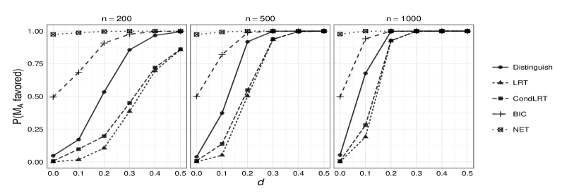
Figure 4: Power associated with test statistics, Simulation 1.

Table 1 contains results associated with 90% confidence intervals of BIC differences. The average interval width, endpoint variability, and coverage are displayed in columns for both the Vuong intervals and nonparametric bootstrap intervals. Rows are based on $n$ and $d$ (the value of the parameter labeled ‘A’ in Figure 1). It is seen that the two types of interval estimates exhibit similar widths and endpoint variability. Coverage is somewhat different, however. When $d$ equals zero, models are indistinguishable and the intervals are invalid. This results in very high coverage rates across both types of intervals. As $d$ initially moves away from zero, both types of intervals exhibit coverage that is too low. Finally, as $d$ gets larger (and as $n$ increases), the intervals converge towards the nominal coverage rate. The bootstrap intervals have a slight advantage here, moving towards a coverage of $0.9$ faster than the Vuong intervals.

Table 1: Average interval widths, variability in endpoints, and coverage of differences in non-nested BICs, Simulation 1.

		Avg Width		Endpoint SD		Coverage
$n$	Path A	Vuong	Boot	Vuong	Boot	Vuong	Boot
200	0	$\phantom{0}8.351$	$10.907$	$\phantom{0}2.952$	$\phantom{0}3.159$	$\phantom{0}0.999$	$\phantom{0}0.995$
	0.1	$11.174$	$13.051$	$\phantom{0}4.277$	$\phantom{0}4.496$	$\phantom{0}0.940$	$\phantom{0}0.979$
	0.2	$17.052$	$17.779$	$\phantom{0}6.092$	$\phantom{0}6.113$	$\phantom{0}0.844$	$\phantom{0}0.883$
	0.3	$23.631$	$23.359$	$\phantom{0}7.846$	$\phantom{0}7.526$	$\phantom{0}0.856$	$\phantom{0}0.884$
	0.4	$29.427$	$28.452$	$\phantom{0}9.401$	$\phantom{0}8.867$	$\phantom{0}0.868$	$\phantom{0}0.885$
	0.5	$33.607$	$32.772$	$10.731$	$10.352$	$\phantom{0}0.857$	$\phantom{0}0.874$
500	0	$\phantom{0}8.256$	$10.697$	$\phantom{0}2.889$	$\phantom{0}3.127$	$\phantom{0}0.999$	$\phantom{0}0.995$
	0.1	$14.460$	$15.762$	$\phantom{0}5.357$	$\phantom{0}5.692$	$\phantom{0}0.846$	$\phantom{0}0.896$
	0.2	$25.645$	$25.939$	$\phantom{0}8.548$	$\phantom{0}8.607$	$\phantom{0}0.861$	$\phantom{0}0.888$
	0.3	$37.184$	$36.880$	$11.690$	$11.438$	$\phantom{0}0.888$	$\phantom{0}0.899$
	0.4	$47.055$	$45.960$	$14.536$	$13.906$	$\phantom{0}0.885$	$\phantom{0}0.895$
	0.5	$53.824$	$52.641$	$16.581$	$16.004$	$\phantom{0}0.890$	$\phantom{0}0.896$
1000	0	$\phantom{0}8.257$	$10.630$	$\phantom{0}2.960$	$\phantom{0}3.193$	$\phantom{0}0.999$	$\phantom{0}0.993$
	0.1	$19.282$	$19.991$	$\phantom{0}6.701$	$\phantom{0}6.986$	$\phantom{0}0.860$	$\phantom{0}0.887$
	0.2	$35.735$	$35.835$	$11.497$	$11.489$	$\phantom{0}0.876$	$\phantom{0}0.891$
	0.3	$52.155$	$51.920$	$16.295$	$16.142$	$\phantom{0}0.895$	$\phantom{0}0.899$
	0.4	$66.860$	$65.839$	$20.507$	$20.017$	$\phantom{0}0.893$	$\phantom{0}0.896$
	0.5	$76.426$	$75.339$	$23.596$	$23.052$	$\phantom{0}0.893$	$\phantom{0}0.900$

In practice, when models are more complex and generally easier to distinguish, the Vuong intervals may exhibit coverage that is more comparable to the bootstrap intervals regardless of $n$. In the following simulation, we study this conjecture.

4 Simulation 2: BIC Intervals

The previous simulation showed that, when candidate models are nearly indistinguishable from one another, interval estimates associated with BIC differences (or with the likelihood ratio) generally stray from the nominal coverage rate. As models become more distinguishable, the intervals initially exhibit coverage that is too high, followed by coverage that is too low, followed by coverage that is just right. In this simulation, we further study the properties of these interval estimates in more complex models that are generally distinguishable from one another. In this situation, the intervals’ coverages should be closer to their advertised coverages.

4.1 Method

The simulation was set up in a manner similar to the simulation from premer12, using the previously-discussed models from Figure 2. These models reflect four unique hypotheses about the relationships between 9 observed variables. One thousand datasets were first generated from Model D, with unstandardized path coefficients being fixed to 0.2, residual variances being fixed to 0.8, and the exogenous variance associated with variable $X_{1}$ being fixed to 1.0. We then fit Models A–C to each dataset and obtained interval estimates of BIC differences. We examined sample sizes of $n=200,500,$ and 1,000 and compared 90% interval estimates from Vuong’s theory to 90% interval estimates from the nonparametric bootstrap. Statistics of interest were those used in Simulation 1: interval coverage, mean interval width, and interval variability.

4.2 Results

Results are displayed in Table 2, with model pairs and sample sizes in rows and interval statistics in columns. The two columns on the right show that coverage is generally good for both methods; the coverages are all close to $.9$. The other columns show that the Vuong intervals tend to be slightly better than the bootstrap intervals: the Vuong widths are slightly smaller, and there is slightly less variability in the endpoints. These small advantages may not be meaningful in many situations, but the results at least show that the bootstrap intervals and Vuong intervals are comparable here. The Vuong intervals have a clear computational advantage, requiring only output from the two fitted models (and no extra data sampling or model fitting). As mentioned previously, the bootstrap intervals may still exhibit better performance when regularity conditions are violated. In the following section, we examine the Vuong statistics’ application to nested model comparison.

Table 2: Average interval widths, variability in endpoints, and coverage of differences in non-nested BICs, Simulation 2.

		Avg Width		Endpoint SD		Coverage
Models	$n$	Vuong	Boot	Vuong	Boot	Vuong	Boot
A-B	200	$39.350$	$42.241$	$12.137$	$12.521$	$\phantom{0}0.919$	$\phantom{0}0.873$
	500	$57.937$	$59.620$	$18.173$	$18.516$	$\phantom{0}0.901$	$\phantom{0}0.875$
	1000	$79.614$	$80.682$	$23.484$	$23.798$	$\phantom{0}0.916$	$\phantom{0}0.907$
B-C	200	$45.469$	$47.805$	$14.508$	$14.885$	$\phantom{0}0.899$	$\phantom{0}0.912$
	500	$69.064$	$70.317$	$20.832$	$21.036$	$\phantom{0}0.901$	$\phantom{0}0.905$
	1000	$95.699$	$96.403$	$29.665$	$29.953$	$\phantom{0}0.893$	$\phantom{0}0.891$
C-A	200	$44.843$	$48.082$	$13.704$	$14.107$	$\phantom{0}0.919$	$\phantom{0}0.894$
	500	$65.386$	$67.320$	$19.633$	$19.853$	$\phantom{0}0.910$	$\phantom{0}0.891$
	1000	$89.381$	$90.753$	$27.655$	$27.977$	$\phantom{0}0.899$	$\phantom{0}0.882$

5 Simulation 3: Tests of Nested Models

When we first introduced the Vuong test statistics, we mentioned that the statistics $n\hat{\omega}^{2}_{*}$ and $2n^{1/2}\text{LR}_{AB}$ provide unique tests of nested models. Unlike the classical likelihood ratio test (also known as the $\chi^{2}$ difference test), tests involving these statistics make no assumption related to the correctness of the full model. In this simulation, we compare the performance of the classical likelihood ratio test of nested models to the Vuong tests involving $n\hat{\omega}^{2}_{*}$ and $2n^{1/2}\text{LR}_{AB}$.

5.1 Method

The data generating model was the path model displayed in Figure 5, where some parameters are represented by solid lines, some parameters are represented by dashed lines, and variance parameters are omitted from the figure. Path coefficients (unstandardized) were set to $0.2$, residual variances were set to $0.8$, and the single exogenous variance was set to $1.0$. The dashed covariance parameters, further described below, were manipulated across conditions. After generating data from this model, we fit two candidate models to the data: the data generating model ($M_{A}$), and a model with the dashed covariance paths omitted ($M_{B}$). The two candidate models are therefore nested, and $M_{A}$ should be preferred when the dashed paths are nonzero. This is a best-case scenario for the traditional likelihood ratio test because the full model ($M_{A}$) is correct.

Figure 5: Path diagrams reflecting the models used in Simulation 3.

Simulation conditions were defined by $n$, which assumed values of 200, 500, and 1,000, and by the value of the dashed covariance parameters, $d$. Within a condition, these covariance parameters simultaneously took values of $0,0.025,0.050,0.075,0.100$, or $0.125$. In each condition, we generated 1,000 datasets and fit both $M_{A}$ and $M_{B}$ to the data. We then computed four statistics: the distinguishability test of (7) (which is actually a test of nested models here), the Vuong LRT involving $2n^{1/2}\text{LR}_{AB}$, the classical LRT based on $\chi^{2}$ differences, and the BIC difference. For each statistic, we recorded whether or not $M_{A}$ was favored over $M_{B}$ using the same criteria that were used in Simulation 1.

5.2 Results

Results are displayed in Figure 6, which is arranged similarly to the figure from Simulation 1. It is seen that power associated with the two Vuong tests is very similar to power associated with the classical LRT (labeled “Chidiff” in the figure), with the distinguishability test exhibiting slightly smaller power at $n=200$. In the $n=500$ and $n=$1,000 conditions, the two Vuong statistics are nearly equivalent to the classical LRT. The BIC, on the other hand, is slower to prefer $M_{A}$ due to the fact that $M_{A}$ has three extra parameters. These extra parameters must be sufficiently far from zero before they are “worth it,” as judged by BIC.

This simulation demonstrates that, within the controlled environment examined here, little is lost if one uses Vuong tests to compare nested models. In some conditions, the Vuong statistics even exhibited slightly higher power than the classical LRT. vuo89 showed that the limiting distributions of his statistics matched the distribution of the classical LRT (when the full model is correctly specified), and our simulation provides evidence that his statistics approach the limiting distribution at a similar rate as the classical LRT. This is relevant to sample size considerations: the Vuong statistics exhibited similar power to the classical LRT, so that we can potentially use classical LRT results to guide us on sample sizes that lead to sufficient power for the Vuong tests. Simulation studies can also be carried out to study the power of the Vuong tests in specific situations.

Future work could compare the Vuong statistics to both the classical LRT and to other robust statistics <see>satben94,sav14 when the candidate models are both incorrect. This is trickier than it sounds, because it is difficult to design a framework that allows us to assess the statistics’ Type I error rates. Such a framework would require that (i) the null hypothesis from (14) holds, and (ii) the data generating model differs from the full model. This framework is necessary so that we know whether or not differences in statistics’ power are paired with differences in statistics’ Type I error rates.

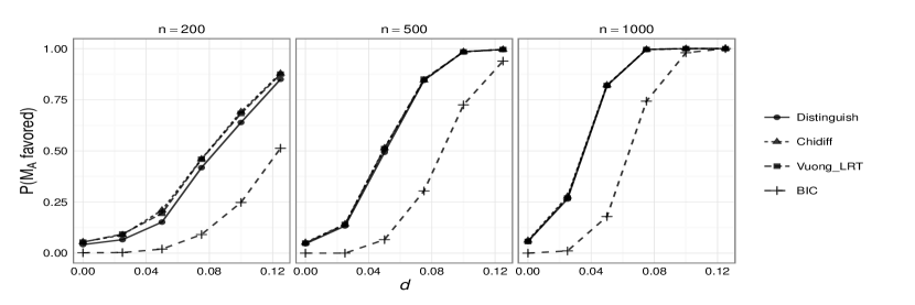
Figure 6: Power associated with test statistics, Simulation 3.

6 General Discussion

The framework described in this paper provides researchers with a general means to test pairs of SEMs for differences in fit. Researchers also gain a means to test whether pairs of SEMs are distinguishable in a population of interest and to test for differences between models’ information criteria. In the discussion below, we provide detail on extension of the tests to comparing multiple ($>2$) models. We also address regularity conditions, extension to other types of models, and a recommended strategy for applied researchers.

Comparing Multiple Models

The reader may wonder whether or not the above theory extends to simultaneously testing multiple models. kat08 derives the joint distribution of LR statistics comparing $(m-1)$ models to a baseline model (i.e., when we have a unique LR statistic comparing each of $(m-1)$ models to the baseline model) and obtains a test statistic based on the sum of the $(m-1)$ squared LR statistics. We do not describe all the details here but instead supply some informal intuition underlying the tests.

In a situation where one wishes to compare multiple models, we can obtain the casewise likelihoods $\ell_{j}(\bm{\theta};x_{i})$, $i=1,\ldots,n$, $j=1,\ldots,m$. We could then subject these casewise likelihoods to an ANOVA, where case ($i$) is a between-subjects factor and model ($j$) is a within-subjects factor. We should expect a main effect of case, because the models will naturally fit some individuals better than others. The main effect of model, however, serves as a test of whether or not all $m$ model fits are equal. Additionally, the error variance informs us of the extent to which models are distinguishable: if the error variance is close to zero, then we have evidence for indistinguishable models. The ANOVA framework could also be useful for posthoc tests, whereby one wishes to specifically know which model fits differ from which others.

We have not implemented the tests derived by Katayama, and the ANOVA described above is not the same as Katayama’s tests. For example, the ANOVA assumes sphericity for the within-subjects “model” factor, whereas Katayama explicitly estimates covariances between model likelihoods. Simultaneous tests of multiple SEMs generally provide interesting directions for future research.

Regularity Conditions

We previously outlined the regularity conditions associated with the Vuong tests, and we expand here on the conditions’ relevance to applied researchers. The conditions under which the Vuong tests hold are fairly general, including existence of second-order derivatives of the log-likelihood, invertibility of the models’ information matrices, and independence and identical distribution of the data vectors $\bm{x}_{i}$. The invertibility requirement can be violated when we apply the distinguishability test to compare mixture models with different numbers of components. This violation is related to the fact that a model with $m-1$ components lies on the boundary of the parameter space of a model with $m$ components. jef03 presents some evidence that this can cause inflated Type I error rates, and wil15 further describes problems with the test’s application to mixture models. At the time of this writing, researchers have generally ignored these issues. Similar issues may arise if one model can be obtained from the other by setting some variance parameters equal to zero. The iid requirement can be violated by certain time series models. This implies that the tests described here may not be applicable to some dynamic SEMs (where $n$ reflects observed timepoints), though rivvuo02 extend the tests to handle these types of models.

Recommended Use

Using the NET and the methods described here <and also in>levhan07,levhan11, one gains a fuller comparison of candidate models. These procedures give researchers the ability to routinely test non-nested models for global equivalence, distinguishability, and differences in fit or information criteria. We recommend the following non-nested model comparison sequence.
 

1. Using the NET, evaluate models for global equivalence (can be done prior to data collection). If models are not found to be equivalent, proceed to 2.

2. Test whether or not models are distinguishable, using the $\omega^{2}_{*}$ statistic (data must have already been collected). If models are found to be distinguishable, proceed to 3.

3. Compare models via the non-nested LRT or a confidence interval of BIC differences.
    
   

If one makes it to the third step, then the test or interval estimate may allow for the preference of one model. Otherwise, we cannot prefer either model to the other. In the case that models are found to be indistinguishable or to have equal fit, follow-up modeling can often be performed to further study the data. For example, one can often specify a larger model that encompasses both candidate models as special cases. This can provide information about important model parameters, which may lead to an alternative model that is a cross between the original candidate models. Overfitting would be a concern associated with this strategy, and it may often be sufficient to simply report results of the encompassing model. Aside from this strategy, however, there is nothing inherently wrong with having indistinguishable or equal-fitting models. Sometimes, there is simply not enough information in the data to differentiate two theories. The above suggested sequence provides more information about the models’ relative standings than do traditional comparisons via BIC, which should help researchers to favor a model only when the data truly favor that model.

Distributional Assumptions

While our current implementation allows researchers to carry out the above steps using SEMs estimated under multivariate normality, extensions to other assumed distributions is immediate. For example, if our observed variables are ordinal, our model may be based on a multinomial distribution. If the model is estimated via ML, then the tests can be carried out as described here; we just need to obtain the “non-standard” model output (casewise contributions to the likelihood, scores) for those models. Researchers often elect to employ alternative discrepancy functions that do not correspond to a specific probability distribution, however, especially when the observed data are discrete. Examples of estimation methods that do not rely on well-defined probability distributions include weighted least squares and pairwise maximum likelihood <e.g.,>katmou12,mut84. Work by gol03 implies that Vuong’s theory can also be applied to models estimated via these alternative discrepancy functions. Further work is needed to obtain the necessary output from models estimated under these functions and to study the tests’ applications.

Finally, we note that the ideas described throughout this paper generally apply to situations where one’s goal is to declare a single model as the best. One may instead wish to average over the set of candidate models, drawing general conclusions across the set <e.g.,>hoemad99. Though it is computationally more difficult, the model averaging strategy allows the researcher to explicitly acknowledge that all of the models in the set are ultimately incorrect.

Computational Details

All results were obtained using the R system for statistical computing R11, version 3.2.0, employing the add-on packages lavaan 0.5-18 lavaan11 for fitting of the models and score computation, nonnest2 0.2 nonnest2 for carrying out the Vuong tests, and simsem 0.5-8 simsempack for simulation convenience functions. R and the packages lavaan, nonnest2, and simsem are freely available under the General Public License 2 from the Comprehensive R Archive Network at http://CRAN.R-project.org/. R code for replication of our results is available at http://semtools.R-Forge.R-project.org/.

Appendix A Tests involving weighted sums of $\chi^{2}$ distributions

In this appendix, we describe technical details underlying the tests whose limiting distributions are weighted sums of $\chi^{2}$ statistics. As stated in the main text, under the hypothesis that $\omega^{2}_{*}=0$, $n\hat{\omega}^{2}_{*}$ converges in distribution to a weighted sum of $(k+q)$ chi-square distributions (with 1 degree of freedom each), where $k$ and $q$ are the number of free parameters in $M_{A}$ and $M_{B}$, respectively. The weights are defined as the squared eigenvalues of a matrix $\bm{W}$, which is defined below. Additionally, for nested or indistinguishable models, $2n^{1/2}\text{LR}_{AB}$ converges in distribution to a similar weighted sum of chi-square distributions, with weights defined as the unsquared eigenvalues of the same matrix $\bm{W}$.

To obtain $\bm{W}$, let the matrices $\bm{U}_{A}(\bm{\theta}_{A})$ and $\bm{V}_{A}(\bm{\theta}_{A})$ be defined as

$$\bm{U}_{A}(\bm{\theta}_{A}) =E\left[\frac{\partial^{2}\ell(\bm{\theta}_{A};\bm{x}_{i})}{\partial\bm{\theta}_{A}\partial\bm{\theta}_{A}^{\prime}}\right]$$

$$\bm{V}_{A}(\bm{\theta}_{A}) =E\left[\frac{\partial\ell(\bm{\theta}_{A};\bm{x}_{i})}{\partial\bm{\theta}_{A}}\cdot\frac{\partial\ell(\bm{\theta}_{A};\bm{x}_{i})}{\partial\bm{\theta}_{A}^{\prime}}\right],$$

which can be obtained from a fitted $M_{A}$’s information matrix and cross-product of scores (see Equations (3) and (4)), respectively. The matrices $\bm{U}_{B}(\bm{\theta}_{B})$ and $\bm{V}_{B}(\bm{\theta}_{B})$ are defined similarly. Further, define $\bm{V}_{AB}(\bm{\theta}_{A},\bm{\theta}_{B})$ as

$$\bm{V}_{AB}(\bm{\theta}_{A},\bm{\theta}_{B})=E\left[\frac{\partial\ell(\bm{\theta}_{A};\bm{x}_{i})}{\partial\bm{\theta}_{A}}\cdot\frac{\partial\ell(\bm{\theta}_{B};\bm{x}_{i})}{\partial\bm{\theta}_{B}^{\prime}}\right],$$

which can be obtained by taking products of ${\bm{s}}(\hat{{\bm{\theta}}}_{A};\bm{x}_{i})$ and ${\bm{s}}(\hat{{\bm{\theta}}}_{B};\bm{x}_{i})$. The matrix $\bm{W}$ is then defined as

$$\bm{W}=\left[\begin{array}[]{cc}-\bm{V}_{A}(\bm{\theta}_{A})\bm{U}^{-1}_{A}(\bm{\theta}_{A})&-\bm{V}_{AB}(\bm{\theta}_{A},\bm{\theta}_{B})\bm{U}^{-1}_{B}(\bm{\theta}_{B})\\ \bm{V}^{\prime}_{AB}(\bm{\theta}_{A},\bm{\theta}_{B})\bm{U}^{-1}_{A}(\bm{\theta}_{A})&\bm{V}_{B}(\bm{\theta}_{B})\bm{U}^{-1}_{B}(\bm{\theta}_{B})\end{array}\right].$$

As stated previously, the eigenvalues of $\bm{W}$ then determine the weights involved in the limiting sum of $\chi^{2}$ distributions. See vuo89 for the proof and further detail.