A stable and linear time discretization for a thermodynamically consistent model for two-phase incompressible flow

Abstract

A new time discretization scheme for the numerical simulation of two-phase flow governed by a thermodynamically consistent diffuse interface model is presented. The scheme is consistent in the sense that it allows for a discrete in time energy inequality. An adaptive spatial discretization is proposed that conserves the energy inequality in the fully discrete setting by applying a suitable post processing step to the adaptive cycle. For the fully discrete scheme a quasi-reliable error estimator is derived which estimates the error both of the flow velocity, and of the phase field. The validity of the energy inequality in the fully discrete setting is numerically investigated.

Introduction

In the present work we propose a stable and (essentially) linear time discretization scheme for two-phase flows governed by the diffuse interface model

$$\rho\partial_{t}v+\left(\left(\rho v+J\right)\cdot\nabla\right)v-\mbox{div}\left(2\eta Dv\right)+\nabla p= \mu\nabla\varphi+\rho g \forall x\in\Omega,\,\forall t\in I,$$ (1)

$$\mbox{div}(v)= 0 \forall x\in\Omega,\,\forall t\in I,$$ (2)

$$\partial_{t}\varphi+v\cdot\nabla\varphi-\mbox{div}(m\nabla\mu)= 0 \forall x\in\Omega,\,\forall t\in I,$$ (3)

$$-\sigma\epsilon\Delta\varphi+F^{\prime}(\varphi)-\mu= 0 \forall x\in\Omega,\,\forall t\in I,$$ (4)

$$v(0,x)= v_{0}(x) \forall x\in\Omega,$$ (5)

$$\varphi(0,x)= \varphi_{0}(x) \forall x\in\Omega,$$ (6)

$$v(t,x)= 0 \forall x\in\partial\Omega,\,\forall t\in I,$$ (7)

$$\nabla\mu(t,x)\cdot\nu_{\Omega}=\nabla\varphi(t,x)\cdot\nu_{\Omega}= 0 \forall x\in\partial\Omega,\,\forall t\in I,$$ (8)

where $J=-\frac{d\rho}{d\varphi}m\nabla\mu$. This model is proposed in [AGG12]. Here $\Omega\subset\mathbb{R}^{n},\,n\in\{2,3\}$, denotes an open and bounded domain, $I=(0,T]$ with $0<T<\infty$ a time interval, $\varphi$ denotes the phase field, $\mu$ the chemical potential, $v$ the volume averaged velocity, $p$ the pressure, and $\rho=\rho(\varphi)=\frac{1}{2}\left((\rho_{2}-\rho_{1})\varphi+(\rho_{1}+\rho_{2})\right)$ the mean density, where $0<\rho_{1}\leq\rho_{2}$ denote the densities of the involved fluids. The viscosity is denoted by $\eta$ and can be chosen arbitrarily, fulfilling $\eta(-1)=\tilde{\eta}_{1}$ and $\eta(1)=\tilde{\eta}_{2}$, with individual fluid viscosities $\eta_{1},\eta_{2}$. The mobility is denoted by $m=m(\varphi)$. The graviational force is denoted by $g$. By $Dv=\frac{1}{2}\left(\nabla v+(\nabla v)^{t}\right)$ we denote the symmetrized gradient. The scaled surface tension is denoted by $\sigma$ and the interfacial width is proportional to $\epsilon$. The free energy is denoted by $F$. For $F$ we use a splitting $F=F_{+}+F_{-}$, where $F_{+}$ is convex and $F_{-}$ is concave.

The above model couples the Navier–Stokes equations (1)–(2) to the Cahn–Hilliard model (3)–(4) in a thermodynamically consistent way, i.e. a free energy inequality holds. It is the main goal to introduce and analyze an (essentially) linear time discretization scheme for the numerical treatment of (1)–(8), which also on the discrete level fulfills the free energy inequality. This in conclusion leads to a stable scheme that is thermodynamically consistent on the discrete level.

Existence of weak solutions to system (1)–(8) for a specific class of free energies $F$ is shown in [ADG13a, ADG13b]. See also the work [Grü13], where the existence of weak solutions for a different class of free energies $F$ is shown by passing to the limit in a numerical scheme. We refer to [LT98], [Boy02], [DSS07], [ADGK13], and the review [AMW98] for other diffuse interface models for two-phase incompressible flow. Numerical approaches for different variants of the Navier–Stokes Cahn–Hilliard system have been studied in [KSW08], [Fen06], [Boy02], [AV12], [Grü13], [HHK13], [GK14] and [GLL].

This work is organized as follows. In Section 1 we derive a weak formulation of (1)–(8) and formulate a time discretization scheme. In Section 2 we derive the fully discrete model and show the existence of solutions for both the time discrete, and the fully discrete model, as well as energy inequalities, both for the time discrete model, and for the fully discrete model. In Section 3 we use the energy inequality to derive a residual based adaptive concept, and in Section 4 we numerically investigate properties of our simulation scheme.

Notation and assumptions

Let $\Omega\subset\mathbb{R}^{n}$, $n\in\{2,3\}$ denote a bounded domain with boundary $\partial\Omega$ and outer normal $\nu_{\Omega}$. Let $I=(0,T)$ denote a time interval.

We use the conventional notation for Sobolev and Hilbert Spaces, see e.g. [AF03]. With $L^{p}(\Omega)$, $1\leq p\leq\infty$, we denote the space of measurable functions on $\Omega$, whose modulus to the power $p$ is Lebesgue-integrable. $L^{\infty}(\Omega)$ denotes the space of measurable functions on $\Omega$, which are essentially bounded. For $p=2$ we denote by $L^{2}(\Omega)$ the space of square integrable functions on $\Omega$ with inner product $(\cdot,\cdot)$ and norm $\|\cdot\|$. For a subset $D\subset\Omega$ and functions $f,g\in L^{2}(\Omega)$ we by $(f,g)_{D}$ denote the inner product of $f$ and $g$ restricted to $D$, and by $\|f\|_{D}$ the respective norm. By $W^{k,p}(\Omega)$, $k\geq 1,1\leq p\leq\infty$, we denote the Sobolev space of functions admitting weak derivatives up to order $k$ in $L^{p}(\Omega)$. If $p=2$ we write $H^{k}(\Omega)$. The subset $H^{1}_{0}(\Omega)$ denotes $H^{1}(\Omega)$ functions with vanishing boundary trace.
We further set

$$L^{2}_{0}(\Omega)=\{v\in L^{2}(\Omega)\,|\,(v,1)=0\},$$

and with

$$H(\mbox{div},\Omega)=\{v\in H^{1}_{0}(\Omega)^{n}\,|\,(\mbox{div}(v),q)=0\,\forall q\in L^{2}_{(0)}(\Omega)\}$$

we denote the space of all weakly solenoidal $H^{1}_{0}(\Omega)$ vector fields.
For $u\in L^{q}(\Omega)^{n}$, $q>n$, and $v,w\in H^{1}(\Omega)^{n}$ we introduce the trilinear form

$$a(u,v,w)=\frac{1}{2}\int_{\Omega}\left(\left(u\cdot\nabla\right)v\right)w\,dx-\frac{1}{2}\int_{\Omega}\left(\left(u\cdot\nabla\right)w\right)v\,dx.$$ (9)

Note that there holds $a(u,v,w)=-a(u,w,v)$, and especially $a(u,v,v)=0$.

For the data of our problem we assume:

1. There exists constants $\overline{\rho}\geq\underline{\rho}>0$, $\overline{\eta}\geq\underline{\eta}>0$, and $\overline{m}\geq\underline{m}>0$ such that the following relations are satisfied:

   • $\overline{\rho}\geq\rho(\varphi)\geq\underline{\rho}>0$,

   • $\overline{\eta}\geq\eta(\varphi)\geq\underline{\eta}>0$,

   • $\overline{m}\geq m(\varphi)\geq\underline{m}>0$.

   Especially we assume that the mobility is non degenerated. In addition we assume, that $\rho$, $\mu$, and $m$ are continuous.

2. $F:\mathbb{R}\to\mathbb{R}$ is continuously differentiable.

3. $F$ and the derivatives $F^{\prime}_{+}$ and $F^{\prime}_{-}$ are polynomially bounded, i.e. there exists $C>0$ such that $|F(x)|\leq C(1+|x|^{q})$, $|F^{\prime}_{+}(x)|\leq C(1+|x|^{q-1})$ and $|F^{\prime}_{-}(x)|\leq C(1+|x|^{q-1})$ holds for some $q\in[1,4]$ if $n=3$ and $q\in[1,\infty)$ if $n=2$,

4. $F^{\prime}_{+}$ is Newton (sometimes called slantly) differentiable (see e.g. [HIK03]) regarded as nonlinear operator $F^{\prime}_{+}:H^{1}(\Omega)\to\left(H^{1}(\Omega)\right)^{*}$ with Newton derivative $G$ satisfying

   $$(G(\varphi)\delta\varphi,\delta\varphi)\geq 0$$

   for each $\varphi\in H^{1}(\Omega)$ and $\delta\varphi\in H^{1}(\Omega)$.

To ensure Assumption A1 we introduce a cut-off mechanism to ensure the bounds on $\rho$ defined in Assumption A1 independently of $\varphi$. Note that $\eta(\varphi)$ and $m(\varphi)$ can be chosen arbitrarily fulfilling the stated bounds. We define the mass density as a smooth, monotone and strictly positive function $\rho(\varphi)$ fulfilling

$$\rho(\varphi)=\begin{cases}\frac{\tilde{\rho}_{2}-\tilde{\rho}_{1}}{2}\varphi+\frac{\tilde{\rho}_{1}+\tilde{\rho}_{2}}{2}&\mbox{ if }-1-\frac{\tilde{\rho}_{1}}{\tilde{\rho}_{2}-\tilde{\rho}_{1}}<\varphi<1+\frac{\tilde{\rho}_{1}}{\tilde{\rho}_{2}-\tilde{\rho}_{1}},\\ \mbox{const}&\mbox{ if }\varphi>1+\frac{2\tilde{\rho}_{1}}{\tilde{\rho}_{2}-\tilde{\rho}_{1}},\\ \mbox{const}&\mbox{ if }\varphi<-1-\frac{2\tilde{\rho}_{1}}{\tilde{\rho}_{2}-\tilde{\rho}_{1}}.\end{cases}$$

For a discussion we refer to [Grü13, Remark 2.1].

Remark 1.

The Assumptions A2–A4 are for example fulfilled by the polynomial free energy

$$F^{poly}(\varphi)=\frac{\sigma}{4\epsilon}\left(1-\varphi^{2}\right)^{2}.$$

Another free energy fulfilling these assumptions is the relaxed double-obstacle free energy given by

$$F^{rel}(\varphi) =\frac{\sigma}{2\epsilon}\left(1-\varphi^{2}+s\lambda^{2}(\varphi)\right),$$ (10)

with

$$\lambda(\varphi) :=\max(0,\varphi-1)+\min(0,\varphi+1),$$

where $s\gg 0$ denotes the relaxation parameter. $F^{rel}$ is introduced in [HHT11] as Moreau–Yosida relaxation of the double-obstacle free energy

$$F^{obst}(\varphi)=\begin{cases}\frac{\sigma}{2\epsilon}\left(1-\varphi^{2}\right)&\mbox{ if }|\varphi|\leq 1,\\ 0&\mbox{ else},\end{cases}$$

which is proposed in [BE91] to model phase separation.

In the numerical examples of this work we use the free energy $F\equiv F^{rel}$. For this choice the splitting into convex and concave part reads

$$F_{+}(\varphi) =s\frac{\sigma}{2\epsilon}\lambda^{2}(\varphi), F_{-}(\varphi) =\frac{\sigma}{2\epsilon}(1-\varphi^{2}).$$

1 The time discrete setting

In the present section we formulate our time discretization scheme that is based on a weak formulation of (1)–(8) which we derive next. To begin with, note that for a sufficiently smooth solution $(\varphi,\mu,v)$ of (1)–(8) we can rewrite (1), using the linearity of $\rho$, as

$$\partial_{t}(\rho v)+\mbox{div}\left(\rho v\otimes v\right)+\mbox{div}\left(v\otimes J\right)-\mbox{div}\left(2\eta Dv\right)+\nabla p=\mu\nabla\varphi+\rho g,$$ (11)

see [AGG12, p. 14].

We also note that the term $\rho v+J$ in (1) is not solenoidal (which might lead to difficulties both in the analytical and the numerical treatment) and that the trilinear form $(((\rho v+J)\cdot\nabla)u,w)$ is not anti-symmetric. To obtain a weak formulation yielding an anti-symmetric convection term we use a convex combination of (1) and (11) to define a weak formulation. We multiply equations (1) and (11) by the solenoidal test function $\frac{1}{2}w\in H(\mbox{div},\Omega)$, integrate over $\Omega$, add the resulting equations and perform integration by parts. This gives

$$\frac{1}{2}\int_{\Omega}\left(\partial_{t}(\rho v)+\rho\partial_{t}v\right)w\,dx+\int_{\Omega}2\eta Dv:Dw\,dx+a(\rho v+J,v,w)=\int_{\Omega}\mu\nabla\varphi w+\rho gw\,dx.$$

Equations (3)–(4) are treated classically. This leads to

Definition 1.

We call $v$, $\varphi$, $\mu$ a weak solution to (1)–(8) if $v(0)=v_{0}$, $\varphi(0)=\varphi_{0}$, $v(t)\in H(\mbox{div},\Omega)$ for $a.e.\,t\in I$ and

$$\frac{1}{2}\int_{\Omega}\left(\partial_{t}(\rho v)+\rho\partial_{t}v\right)w\,dx+\int_{\Omega}2\eta Dv:Dw\,dx$$

$$+a(\rho v+J,v,w)=\int_{\Omega}\mu\nabla\varphi w+\rho gw\,dx \quad\forall w\in H(\mbox{div},\Omega),$$ (12)

$$\int_{\Omega}\left(\partial_{t}\varphi+v\cdot\nabla\varphi\right)\Phi\,dx+\int_{\Omega}m(\varphi)\nabla\mu\cdot\nabla\Phi\,dx=0 \quad\forall\Phi\in H^{1}(\Omega),$$ (13)

$$\sigma\epsilon\int_{\Omega}\nabla\varphi\cdot\nabla\Psi\,dx+\int_{\Omega}F^{\prime}(\varphi)\Psi\,dx-\int_{\Omega}\mu\Psi\,dx=0 \quad\forall\Psi\in H^{1}(\Omega),$$ (14)

is satisfied for almost all $t\in I$.

Theorem 1.

Let $v,\varphi,\mu$ be a sufficiently smooth solution to (12)–(14). Then there holds

$$\frac{1}{2}\frac{d}{dt}\left(\int_{\Omega}\rho|v|^{2}+\sigma\epsilon|\nabla\varphi|^{2}+F(\varphi)\,dx\right)=-\int_{\Omega}2\eta|Dv|^{2}+m|\nabla\mu|^{2}\,dx+\int_{\Omega}\rho gv\,dx.$$

Proof.

By testing (12) with $w\equiv v$, (13) with $\Phi\equiv\mu$ and (14) with $\Psi\equiv\partial_{t}\varphi$ and adding the resulting equations the claim follows. ∎

In [ADG13a, ADG13b] an alternative weak formulation of (1)–(8) is proposed, for which the authors show existence of weak solutions.

We now introduce a time discretization which mimics the energy inequality in Theorem 1 on the discrete level. Let $0=t_{0}<t_{1}<\ldots<t_{k-1}<t_{k}<t_{k+1}<\ldots<t_{M}=T$ denote an equidistant subdivision of the interval $\overline{I}=[0,T]$ with $\tau_{k+1}-\tau_{k}=\tau$. From here onwards the superscript $k$ denotes the corresponding variables at time instance $t_{k}$.

Time integration scheme
Let $\varphi_{0}\in H^{1}(\Omega)$ and $v_{0}\in H(\mbox{div},\Omega)$.

Initialization for $k=0$:
Set $\varphi^{0}=\varphi_{0}$ and $v^{0}=v_{0}$.
Find $\varphi^{1}\in H^{1}(\Omega)$, $\mu^{1}\in H^{1}(\Omega)$, $v^{1}\in H(\mbox{div},\Omega)$, such that for all $w\in H(\mbox{div},\Omega)$, $\Phi\in H^{1}(\Omega)$, and $\Psi\in H^{1}(\Omega)$ it holds

$$\frac{1}{\tau}\int_{\Omega}\rho^{1}(v^{1}-v^{0})w\,dx+\int_{\Omega}((\rho^{0}v^{0}+J^{1})\cdot\nabla)v^{1}\cdot w\,dx$$

$$+\int_{\Omega}2\eta^{1}Dv^{1}:Dw\,dx-\int_{\Omega}\mu^{1}\nabla\varphi^{1}w+\rho^{1}gw\,dx =0 \forall w\in H(\mbox{div},\Omega),$$ (15)

$$\frac{1}{\tau}\int_{\Omega}(\varphi^{1}-\varphi^{0})\Phi\,dx+\int_{\Omega}(v^{0}\cdot\nabla\varphi^{0})\Phi\,dx$$

$$+\int_{\Omega}m(\varphi^{0})\nabla\mu^{1}\cdot\nabla\Phi\,dx =0 \forall\Phi\in H^{1}(\Omega),$$ (16)

$$\sigma\epsilon\int_{\Omega}\nabla\varphi^{1}\cdot\nabla\Psi\,dx-\int_{\Omega}\mu^{1}\Psi\,dx$$

$$+\int_{\Omega}((F_{+})^{\prime}(\varphi^{1})+(F_{-})^{\prime}(\varphi^{0}))\Psi\,dx =0 \forall\Psi\in H^{1}(\Omega),$$ (17)

where $J^{1}:=-\frac{d\rho}{d\varphi}(\varphi^{1})m^{1}\nabla\mu^{1}$.

Two-step scheme for $k\geq 1$:
Given $\varphi^{k-1}\in H^{1}(\Omega)$, $\varphi^{k}\in H^{1}(\Omega)$, $\mu^{k}\in W^{1,q}(\Omega)$, $q>n$, $v^{k}\in H(\mbox{div},\Omega)$,
find $v^{k+1}\in H(\mbox{div},\Omega)$, $\varphi^{k+1}\in H^{1}(\Omega)$, $\mu^{k+1}\in H^{1}(\Omega)$ satisfying

$$\frac{1}{2\tau}\int_{\Omega}\left(\rho^{k}v^{k+1}-\rho^{k-1}v^{k}\right)w+\rho^{k-1}(v^{k+1}-v^{k})w\,dx$$

$$+a(\rho^{k}v^{k}+J^{k},v^{k+1},w)+\int_{\Omega}2\eta^{k}Dv^{k+1}:Dw\,dx$$

$$-\int_{\Omega}\mu^{k+1}\nabla\varphi^{k}w-\rho^{k}gw\,dx =0 \forall w\in H(\mbox{div},\Omega),$$ (18)

$$\frac{1}{\tau}\int_{\Omega}(\varphi^{k+1}-\varphi^{k})\Phi\,dx+\int_{\Omega}(v^{k+1}\cdot\nabla\varphi^{k})\Phi\,dx$$

$$+\int_{\Omega}m(\varphi^{k})\nabla\mu^{k+1}\cdot\nabla\Phi\,dx =0 \forall\Phi\in H^{1}(\Omega),$$ (19)

$$\sigma\epsilon\int_{\Omega}\nabla\varphi^{k+1}\cdot\nabla\Psi\,dx-\int_{\Omega}\mu^{k+1}\Psi\,dx$$

$$+\int_{\Omega}((F_{+})^{\prime}(\varphi^{k+1})+(F_{-})^{\prime}(\varphi^{k}))\Psi\,dx =0 \forall\Psi\in H^{1}(\Omega),$$ (20)

where $J^{k}:=-\frac{d\rho}{d\varphi}(\varphi^{k})m^{k}\nabla\mu^{k}$.

We note that in (18)–(20) the only nonlinearity arises from $F_{+}^{\prime}$ and thus only the equation (20) is nonlinear. Let us summarize properties of this scheme in the following remark.

Remark 2.

• The time discretization (15)–(17) used in the initialization step is motivated by the time discretization in [KSW08] for the equal density case. In particular it yields a sequential coupling of the Cahn–Hilliard and the Navier–Stokes systems. Concerning the existence of a unique solution we refer to e.g. [HHK13]. From the regularity theory for the Laplace operator we have $\mu^{1}\in H^{2}(\Omega)$.

• Existence and uniqueness of a solution to the time discrete model (18)–(20) is shown in Theorem 6. Using the Assumption A4 posed on $F$, it can be shown that Newton’s method in function space can be used to compute a solution to (18)–(20) using the steps from Theorem 6.

• Through the use of $\rho^{k-1}$, (18)–(20) is a 2-step scheme. However, by replacing (18) with

  $$\frac{1}{2\tau}\int_{\Omega}\left(\rho^{k+1}v^{k+1}-\rho^{k}v^{k}\right)w+\rho^{k}(v^{k+1}-v^{k})w\,dx$$

  $$+a(\rho^{k}v^{k}+J^{k},v^{k+1},w)+\int_{\Omega}2\eta Dv^{k+1}:Dw\,dx$$

  $$-\int_{\Omega}\mu^{k+1}\nabla\varphi^{k}w+\rho^{k}gw\,dx =0\quad\forall w\in H(\mbox{div},\Omega),$$

  one obtains an one-step scheme, which then also is nonlinear in the time discretization of (12). The resulting system is analyzed in a forthcoming paper.

In [GK14] Grün and Klingbeil propose a time-discrete solver for (1)–(8) which leads to strongly coupled systems for $v,\varphi$ and $p$ at every time step and requires a fully nonlinear solver. For this scheme Grün in [Grü13] proves an energy inequality and the existence of so called generalized solutions.

2 The fully discrete setting and energy inequalities

For a numerical treatment we next discretize the weak formulation (18)–(20) in space. We aim at an adaptive discretization of the domain $\Omega$, and thus to have a different spatial discretization in every time step.

Let $\mathcal{T}^{k}=\bigcup_{i=1}^{NT}T_{i}$ denote a conforming triangulation of $\overline{\Omega}$ with closed simplices $T_{i},i=1,\ldots,NT$ and edges $E_{i},i=1,\ldots,NE$, $\mathcal{E}^{k}=\bigcup_{i=1}^{NE}E_{i}$. Here $k$ refers to the time instance $t_{k}$. On $\mathcal{T}^{k}$ we define the following finite element spaces:

$$\mathcal{V}^{1}(\mathcal{T}^{k})= \{v\in C(\mathcal{T}^{k})\,|\,v|_{T}\in P^{1}(T)\,\forall T\in\mathcal{T}^{k}\}=:\mbox{span}\{\Phi^{i}\}_{i=1}^{NP},$$

$$\mathcal{V}^{2}(\mathcal{T}^{k})= \{v\in C(\mathcal{T}^{k})\,|\,v|_{T}\in P^{2}(T)\,\forall T\in\mathcal{T}^{k}\},$$

where $P^{l}(S)$ denotes the space of polynomials up to order $l$ defined on $S$.

We introduce the discrete analogon to the space $H(\mbox{div},\Omega)$:

$$H(\mbox{div},\mathcal{T}^{k}) =\{v\in\mathcal{V}^{2}(\mathcal{T}^{k})^{n}\,|\,(\mbox{div}v,q)=0\,\forall q\in\mathcal{V}^{1}(\mathcal{T}^{k})\cap L^{2}_{(0)}(\Omega),\,v|_{\partial\Omega}=0\}$$

$$:=\mbox{span}\{b^{i}\}_{i=1}^{NF},$$

We further introduce a $H^{1}$-stable projection operator $\mathcal{P}^{k}:H^{1}(\Omega)\to\mathcal{V}^{1}(\mathcal{T}^{k})$ satisfying

$$\|\mathcal{P}^{k}v\|_{L^{p}(\Omega)}\leq\|v\|_{L^{p}(\Omega)}\mbox{ and }\|\nabla\mathcal{P}^{k}v\|_{L^{r}(\Omega)}\leq\|\nabla v\|_{L^{r}(\Omega)}$$

for $v\in H^{1}(\Omega)$ with $r\in[1,2]$ and $p\in[1,6)$ if $n=3$, and $p\in[1,\infty)$ if $n=2$. Possible choices are the Clément operator ([Clé75]) or, by restricting the preimage to $C(\overline{\Omega})\cap H^{1}(\Omega)$, the Lagrangian interpolation operator.

Using these spaces we state the discrete counterpart of (18)–(20):

Let $k\geq 1$, given $\varphi^{k-1}\in\mathcal{V}^{1}(\mathcal{T}^{k-1})$, $\varphi^{k}\in\mathcal{V}^{1}(\mathcal{T}^{k})$, $\mu^{k}\in\mathcal{V}^{1}(\mathcal{T}^{k})$, $v^{k}\in H(\mbox{div},\mathcal{T}^{k})$, find $v^{k+1}_{h}\in H(\mbox{div},\mathcal{T}^{k+1})$, $\varphi^{k+1}_{h}\in\mathcal{V}^{1}(\mathcal{T}^{k+1})$, $\mu^{k+1}_{h}\in\mathcal{V}^{1}(\mathcal{T}^{k+1})$ such that for all $w\in H(\mbox{div},\mathcal{T}^{k+1})$, $\Phi\in\mathcal{V}^{1}(\mathcal{T}^{k+1})$, $\Psi\in\mathcal{V}^{1}(\mathcal{T}^{k+1})$ there holds:

$$\frac{1}{2\tau}(\rho^{k}v^{k+1}_{h}-\rho^{k-1}v^{k}+\rho^{k-1}(v^{k+1}_{h}-v^{k}),w)+a(\rho^{k}v^{k}+J^{k},v_{h}^{k+1},w)$$

$$+(2\eta^{k}Dv^{k+1}_{h},Dw)-(\mu^{k+1}_{h}\nabla\varphi^{k}+\rho^{k}g,w) =0,$$ (21)

$$\frac{1}{\tau}(\varphi^{k+1}_{h}-\mathcal{P}^{k+1}\varphi^{k},\Phi)+(m(\varphi^{k})\nabla\mu^{k+1}_{h},\nabla\Phi)+(v^{k+1}_{h}\nabla\varphi^{k},\Phi) =0,$$ (22)

$$\sigma\epsilon(\nabla\varphi^{k+1}_{h},\nabla\Psi)+(F_{+}^{\prime}(\varphi^{k+1}_{h})+F^{\prime}_{-}(\mathcal{P}^{k+1}\varphi^{k}),\Psi)-(\mu^{k+1}_{h},\Psi) =0,$$ (23)

where $\varphi^{0}=P\varphi_{0}$ denotes the $L^{2}$ projection of $\varphi_{0}$ in $\mathcal{V}^{1}(\mathcal{T}^{0})$, $v^{0}=P^{L}v_{0}$ denotes the Leray projection of $v_{0}$ in $H(\mbox{div},\mathcal{T}^{0})$ (see [CF88]), and $\varphi_{h}^{1},\mu_{h}^{1},v_{h}^{1}$ are obtained from the fully discrete variant of (15)–(17).

2.1 Existence of solution to the fully discrete system

We next show the existence of a unique solution to the fully discrete system (21)–(23).

Theorem 2.

There exist $v^{k+1}_{h}\in H(\mbox{div},\mathcal{T}^{k+1})$, $\varphi^{k+1}_{h}\in\mathcal{V}^{1}(\mathcal{T}^{k+1})$, $\mu^{k+1}_{h}\in\mathcal{V}^{1}(\mathcal{T}^{k+1})$ solving (21)–(23).

Proof.

By testing (22) with $\Phi\equiv 1$, integration by parts in $(v^{k+1}_{h}\nabla\varphi^{k},1)$ and using $v^{k+1}_{h}\in H(\mbox{div},\mathcal{T}^{k+1})$ we obtain

$$(\varphi^{k+1}_{h},1)=(\mathcal{P}^{k+1}\varphi^{k},1).$$

We define $\alpha=\frac{1}{|\Omega|}\int_{\Omega}\mathcal{P}^{k+1}\varphi^{k}\,dx$ and set

$$V_{(0)}:=\{v_{h}\in\mathcal{V}^{1}(\mathcal{T}^{k+1})\,\mid\,(v_{h},1)=0\}.$$

Then $z^{k+1}:=\varphi^{k+1}-\alpha$ fulfills $z^{k+1}\in V_{(0)}$. In the following we use $z^{k+1}$ as unknown for the phase field, since the mean value of $\varphi$ is fixed. In addition we introduce $y^{k+1}:=\mu^{k+1}_{h}-\frac{1}{|\Omega|}\int\mu^{k+1}_{h}\,dx$ and require (22)–(23) preliminarily only for test functions with zero mean value.

We define

$$X=H(\mbox{div},\mathcal{T}^{k+1})\times V_{(0)}\times V_{(0)},$$

with the inner product

$$\left((v_{1},y_{1},z_{1}),(v_{2},y_{2},z_{2})\right)_{X}:=(Dv_{1},Dv_{2})+(\nabla y_{1},\nabla y_{2})+(\nabla z_{1},\nabla z_{2}),$$

and norm $\|\cdot\|_{X}^{2}=(\cdot,\cdot)_{X}$. It follows from the inequalities of Korn and Poincaré that $(\cdot,\cdot)_{X}$ indeed forms an inner product on $X$. For $(v,y,z)\in X$ we define

$$\left(G(v,y,z),(\overline{v},\overline{y},\overline{z})\right)_{X}:= \left(\frac{1}{2}(\rho^{k}+\rho^{k-1})v-\rho^{k-1}v^{k},\overline{v}\right)+\tau a(\rho^{k}v^{k}+J^{k},v,\overline{v})$$

$$+\tau(2\eta^{k}Dv,D\overline{v})-\tau(y\nabla\varphi^{k},\overline{v})-\tau(\rho^{k}g,\overline{v})$$

$$+(z-\mathcal{P}^{k+1}\varphi^{k},\overline{y})+\tau(m(\varphi^{k})\nabla y,\nabla\overline{y})+\tau(v\nabla\varphi^{k},\overline{y})$$

$$+\sigma\epsilon(\nabla z,\nabla\overline{z})+(F^{\prime}_{+}(z+\alpha)+F^{\prime}_{-}(\mathcal{P}^{k+1}\varphi^{k}),\overline{z})-(y,\overline{z}).$$

Now we show $(G(v,y,z),(v,y,z))_{X}>0$ for $\|(v,y,z)\|_{X}$ large enough and that $G$ satisfies the supposition of [Tem77, Lem. II.1.4]. It then follows from [Tem77, Lem. II.1.4], that $G$ admits a root $(v^{*},y^{*},z^{*})\in X$.

The function $G$ is obviously continuous. We now estimate

$$(G(v,y,z),(v,y,z))_{X}\geq \,\underline{\rho}(v,v)+2\tau\underline{\eta}(Dv,Dv)$$ (24)

$$+\tau\underline{m}(\nabla y,\nabla y)+\sigma\epsilon(\nabla z,\nabla z)+(F^{\prime}_{+}(z+\alpha),z)$$

$$-(\rho^{k-1}v^{k},v)-\tau(\rho^{k}g,v)-(\mathcal{P}^{k+1}\varphi^{k},y)+(F^{\prime}_{-}(\mathcal{P}^{k+1}\varphi^{k}),z).$$

Using the convexity of $F_{+}$, which implies that $F_{+}^{\prime}$ is monotone, we obtain

$$(F^{\prime}_{+}(z+\alpha),z)=(F^{\prime}_{+}(z+\alpha)-F^{\prime}_{+}(\alpha),z)+(F^{\prime}_{+}(\alpha),z)\geq(F^{\prime}_{+}(\alpha),z).$$

By using Hölder’s and Poincaré’s inequality in (24) we obtain

$$(G(v,y,z),(v,y,z))_{X}>0$$

for $\|(v,y,z)\|_{X}\geq R$ if $R$ is large enough. Now [Tem77, Lem. II.1.4] implies the existence of $(v^{*},y^{*},z^{*})\in X$ such that $G(v^{*},y^{*},z^{*})=0$. Defining $(v,\mu,\varphi)=(v^{*},y^{*}+\beta,z^{*}+\alpha)$ with $\beta$ such that $(\beta,1)=(F^{\prime}_{+}(\varphi)+F^{\prime}_{-}(\mathcal{P}^{k+1}\varphi^{k}),1)$ we obtain that $(v,\mu,\varphi)$ solves (21)–(23). ∎

Remark 3.

Note that we do not need that the variables from old time instances are defined on the mesh used on the current time instance. We further do not need any smallness requirement on the mesh size $h$ or on the time step length $\tau$.

Theorem 3.

Let $(\varphi^{k+1}_{h}$, $\mu_{h}^{k+1}$, $v_{h}^{k+1})$ be a solution to (21)–(23). Then for $k\geq 1$:

$$\frac{1}{2}\int_{\Omega}\rho^{k}\left|v^{k+1}_{h}\right|^{2}\,dx+\frac{\sigma\epsilon}{2}\int_{\Omega}|\nabla\varphi^{k+1}_{h}|^{2}\,dx+\int_{\Omega}F(\varphi^{k+1}_{h})\,dx$$

$$+\frac{1}{2}\int_{\Omega}\rho^{k-1}|v^{k+1}_{h}-v^{k}|^{2}\,dx+\frac{\sigma\epsilon}{2}\int_{\Omega}|\nabla\varphi^{k+1}_{h}-\nabla\mathcal{P}^{k+1}\varphi^{k}|^{2}\,dx$$

$$+\tau\int_{\Omega}2\eta^{k}|Dv^{k+1}_{h}|^{2}\,dx+\tau\int_{\Omega}m^{k}|\nabla\mu^{k+1}_{h}|^{2}\,dx$$

$$\leq\frac{1}{2}\int_{\Omega}\rho^{k-1}\left|v^{k}\right|^{2}\,dx+\frac{\sigma\epsilon}{2}\int_{\Omega}|\nabla\mathcal{P}^{k+1}\varphi^{k}|^{2}\,dx+\int_{\Omega}F(\mathcal{P}^{k+1}\varphi^{k})\,dx+\tau\int_{\Omega}\rho^{k}gv^{k+1}_{h}.$$ (25)

Proof.

We have

$$\frac{1}{2}\left(\rho^{k}v_{h}^{k+1}-\rho^{k-1}v^{k}\right)\cdot v_{h}^{k+1}+\frac{1}{2}\rho^{k-1}\left(v_{h}^{k+1}-v^{k}\right)\cdot v_{h}^{k+1}$$

$$=\frac{1}{2}\rho^{k}\left|v_{h}^{k+1}\right|^{2}+\frac{1}{2}\rho^{k-1}\left|v_{h}^{k+1}-v^{k}\right|^{2}-\frac{1}{2}\rho^{k-1}\left|v^{k}\right|^{2},$$ (26)

$$\nabla\varphi_{h}^{k+1} \cdot\left(\nabla\varphi_{h}^{k+1}-\nabla\varphi^{k}\right)$$

$$= \frac{1}{2}|\nabla\varphi_{h}^{k+1}|^{2}-\frac{1}{2}|\nabla\varphi^{k}|^{2}+\frac{1}{2}|\nabla\varphi_{h}^{k+1}-\nabla\varphi^{k}|^{2},$$ (27)

and since $F_{+}$ is convex and $F_{-}$ is concave,

$$F_{+}(\varphi_{h}^{k+1})-F_{+}(\varphi^{k}) \leq F^{\prime}_{+}(\varphi_{h}^{k+1})(\varphi_{h}^{k+1}-\varphi^{k}),$$ (28)

$$F_{-}(\varphi_{h}^{k+1})-F_{-}(\varphi^{k}) \leq F^{\prime}_{-}(\varphi^{k})(\varphi_{h}^{k+1}-\varphi^{k}).$$ (29)

The inequality is now obtained from testing (18) with $v_{h}^{k+1}$, (19) with $\mu_{h}^{k+1}$, (20) with $(\varphi_{h}^{k+1}-\mathcal{P}^{k+1}\varphi^{k})/\tau$, and adding the resulting equations. This leads to

$$\frac{1}{2\tau}(\rho^{k}v_{h}^{k+1}-\rho^{k-1}v^{k},v_{h}^{k+1})+\frac{1}{2\tau}(\rho^{k-1}(v_{h}^{k+1}-v^{k}),v_{h}^{k+1})$$

$$+a(\rho^{k}v+J^{k},v_{h}^{k+1},v_{h}^{k+1})+(2\eta^{k}Dv_{h}^{k+1}:Dv_{h}^{k+1})-(\mu_{h}^{k+1}\nabla\varphi^{k},v_{h}^{k+1})$$

$$+\frac{1}{\tau}(\varphi_{h}^{k+1}-\mathcal{P}^{k+1}\varphi^{k},\mu_{h}^{k+1})+(v_{h}^{k+1}\nabla\varphi^{k},\mu_{h}^{k+1})+(m^{k}\nabla\mu_{h}^{k+1},\nabla\mu_{h}^{k+1})$$

$$+\sigma\epsilon\frac{1}{\tau}(\nabla\varphi_{h}^{k+1},\nabla(\varphi_{h}^{k+1}-\mathcal{P}^{k+1}\varphi^{k}))-\frac{1}{\tau}(\mu_{h}^{k+1},\varphi_{h}^{k+1}-\mathcal{P}^{k+1}\varphi^{k})$$

$$+\frac{1}{\tau}(F^{\prime}_{+}(\varphi_{h}^{k+1}),\varphi_{h}^{k+1}-\mathcal{P}^{k+1}\varphi^{k})+\frac{1}{\tau}(F^{\prime}_{-}(\varphi^{k}),\varphi_{h}^{k+1}-\mathcal{P}^{k+1}\varphi^{k})$$

$$-(\rho^{k}g,v^{k+1}_{h}) =0.$$

The equalities (26) and (27) and the inequalities (28) and (29) now imply

$$\frac{1}{2\tau}\int_{\Omega}\left(\rho^{k}|v_{h}^{k+1}|^{2}+\rho^{k-1}|v_{h}^{k+1}-v^{k}|^{2}-\rho^{k-1}|v^{k}|^{2}\right)\,dx$$

$$+\int_{\Omega}2\eta^{k}|Dv_{h}^{k+1}|^{2}\,dx+\int_{\Omega}m^{k}|\nabla\mu_{h}^{k+1}|^{2}\,dx$$

$$+\frac{\sigma\epsilon}{2\tau}\int_{\Omega}|\nabla\varphi_{h}^{k+1}|^{2}\,dx-\frac{\sigma\epsilon}{2\tau}\int_{\Omega}|\nabla\mathcal{P}^{k+1}\varphi^{k}|^{2}\,dx+\frac{\sigma\epsilon}{2\tau}\int_{\Omega}|\nabla\varphi_{h}^{k+1}-\nabla\mathcal{P}^{k+1}\varphi^{k}|^{2}\,dx$$

$$+\frac{1}{\tau}\int_{\Omega}\left(F(\varphi_{h}^{k+1})-F(\mathcal{P}^{k+1}\varphi^{k})\right)\,dx-\int_{\Omega}\rho^{k}gv^{k+1}_{h}\,dx \leq 0,$$

which is the claim. ∎

Theorem 4.

System (21)–(23) admits a unique solution.

Proof.

Assume there exist two different solutions to (21)–(23) denoted by $(v^{1},\varphi^{1},\mu^{1})$ and $(v^{2},\varphi^{2},\mu^{2})$. We show that the difference $v=v^{1}-v^{2},\varphi=\varphi^{1}-\varphi^{2},\mu=\mu^{1}-\mu^{2}$ is zero.

After inserting the two solutions into (21)–(23) and substracting the two sets of equations we perform the same steps as for the derivation of the discrete energy estimate, Theorem 3, and obtain

$$0= \frac{1}{2}\int_{\Omega}(\rho^{k}+\rho^{k-1})v^{2}\,dx+2\tau\int_{\Omega}\eta^{k}|Dv|^{2}\,dx$$

$$+\tau\|\sqrt{m^{k}}\nabla\mu\|^{2}+\sigma\epsilon\|\nabla\varphi\|^{2}+\left(F^{\prime}_{+}(\varphi^{1})-F_{+}^{\prime}(\varphi^{2}),\varphi^{1}-\varphi^{2}\right).$$

Since all these terms are non negative we obtain

$$\frac{1}{2}\int_{\Omega}(\rho^{k}+\rho^{k-1})v^{2}\,dx= 0, \int_{\Omega}\eta^{k}|Dv|^{2}\,dx= 0,$$

$$\|\nabla\mu\|^{2}= 0, \|\nabla\varphi\|^{2}= 0.$$

Since both $\eta(\cdot)$ and $\rho(\cdot)$ are strictly positive by Assumption A1 we conclude $\|v\|_{H^{1}(\Omega)^{n}}=0$ and thus the uniqueness of the velocity field.

By testing (22) by $\Phi\equiv 1$ we obtain $(\varphi^{1},1)=(\varphi^{2},1)=(\mathcal{P}^{k+1}\varphi^{k},1)$ and thus $(\varphi^{1}-\varphi^{2},1)=0$. Poincaré-Friedrichs inequality then yields $\|\varphi\|_{H^{1}(\Omega)}=0$, and thus the uniqueness of the phase field.

Last we directly obtain that the chemical potential is unique up to a constant. By testing (23) with $\Psi\equiv 1$ and inserting the two solutions we obtain $(\mu^{1}-\mu^{2},1)=(F_{+}^{\prime}(\varphi^{1})-F_{+}^{\prime}(\varphi^{2}),1)=0$ and thus $\|\mu\|_{H^{1}(\Omega)}=0$, again by using Poincaré-Friedrichs inequality. ∎

Theorem 3 estimates the Ginzburg Landau energy of the current phase field $\varphi^{k+1}$ against the Ginzburg Landau energy of the projection of the old phase field $\mathcal{P}^{k+1}(\varphi^{k})$. Our aim is to obtain global in time inequalities estimating the energy of the new phase field against the energy of the old phase field at each time step. For this purpose let us state an assumption that later will be justified.

Assumption 1.

Let $\varphi^{k}\in\mathcal{V}^{1}(\mathcal{T}^{k})$ denote the phase field at time instance $t_{k}$. Let $\mathcal{P}^{k+1}\varphi^{k}\in\mathcal{V}^{1}(\mathcal{T}^{k+1})$ denote the projection of $\varphi^{k}$ in $\mathcal{V}^{1}(\mathcal{T}^{k+1})$. We assume that there holds

$$F(\mathcal{P}^{k+1}\varphi^{k})+\frac{1}{2}\sigma\epsilon|\nabla\mathcal{P}^{k+1}\varphi^{k}|^{2}\leq F(\varphi^{k})+\frac{1}{2}\sigma\epsilon|\nabla\varphi^{k}|^{2}.$$ (30)

This assumption means, that the Ginzburg Landau energy is not increasing through projection. Thus no energy is numerically produced.

Assumption 1 is in general not fulfilled for arbitrary sequences $(\mathcal{T}^{k+1})$ of triangulations. To ensure (30) we add a post processing step to the adaptive space meshing, see Section 3.

Theorem 5.

Assume that for every $k=0,1,\ldots$ Assumption 1 holds. Then for every $1\leq k<l$ we have

$$\frac{1}{2}(\rho^{k-1}_{h}v^{k}_{h},v^{k}_{h})+ \int_{\Omega}F(\varphi^{k}_{h})\,dx+\frac{1}{2}\sigma\epsilon(\nabla\varphi^{k}_{h},\nabla\varphi^{k}_{h})+\tau\sum_{m=k}^{l-1}(\rho^{m}g,v_{h}^{m+1})$$

$$\geq\frac{1}{2}(\rho^{l-1}v^{l}_{h},v^{l}_{h})+\int_{\Omega}F(\varphi^{l}_{h})\,dx+\frac{1}{2}\sigma\epsilon(\nabla\varphi^{l}_{h},\nabla\varphi^{l}_{h})$$

$$+\sum_{m=k}^{l-1}(\rho^{m-1}(v^{m+1}_{h}-v^{m}_{h}),(v^{m+1}_{h}-v^{m}_{h}))$$

$$+\tau\sum_{m=k}^{l-1}(2\eta^{m}Dv^{m+1}_{h},Dv^{m+1}_{h})$$

$$+\tau\sum_{m=k}^{l-1}(m(\varphi^{m}_{h})\nabla\mu^{m+1}_{h},\nabla\mu^{m+1}_{h})$$

$$+\frac{1}{2}\sigma\epsilon\sum_{m=k}^{l-1}(\nabla\varphi^{m+1}_{h}-\nabla\mathcal{P}^{m+1}\varphi^{m}_{h},\nabla\varphi^{m+1}_{h}-\nabla\mathcal{P}^{m+1}\varphi^{m}_{h}).$$

Proof.

The stated result is obtained immediately from the energy estimate over one time step (3) together with the Assumption 1. ∎

Remark 4.

We note that using $\Phi=1$ in (22) and using integration by parts only delivers $(\varphi^{k+1}_{h},1)=(\mathcal{P}^{k+1}\varphi^{k},1)$ instead of $(\varphi^{k+1}_{h},1)=(\varphi^{k},1)$. If we use the quasi interpolation operator $Q^{k+1}$ introduced by Carstensen in [Car99] for our generic projection $\mathcal{P}^{k+1}$, we would obtain $(\varphi^{k+1}_{h},1)=(\varphi^{k},1)$ since $Q^{k+1}$ preserves the mean value, i.e. $(\varphi^{k+1}_{h},1)=(Q^{k+1}\varphi^{k},1)$ $\forall\varphi\in L^{1}(\Omega)$.

On the other hand if we use Lagrange interpolation $I^{k+1}$ we have $|(I^{k+1}\varphi^{k},1)_{T}-(\varphi^{k},1)_{T}|\leq Ch_{T}^{3}\|\varphi^{k}\|_{T}$, and the deviation of $(I^{k+1}\varphi^{k},1)$ from $(\varphi^{k},1)$ remaines small if we use bisection as refinement strategy, since then $I^{k+1}\varphi^{k}\in\mathcal{V}^{1}(\mathcal{T}^{k+1})$ and $\varphi^{k}\in\mathcal{V}^{1}(\mathcal{T}^{k})$ only differ on coarsened patches.

2.2 Existence of a solution to the time discrete system

Now we have shown that there exists a unique solution to (21)–(23). The energy inequality can be used to obtain uniform bounds on the solution and will be used to obtain a solution to the time discrete system (18)–(20) by a Galerkin method.

Theorem 6.

Let $v^{k}\in H(\mbox{div},\Omega)$, $\varphi^{k-1}\in H^{1}(\Omega)$, $\varphi^{k}\in H^{1}(\Omega)$, and $\mu^{k}\in W^{1,q}(\Omega),q>n$ be given data. Then there exists a weak solution to (18)–(20). Moreover, $\varphi^{k+1}\in H^{2}(\Omega)$ and $\mu^{k+1}\in H^{2}(\Omega)$ holds.

Proof.

We proceed as follows. We construct a sequence of meshes $(\mathcal{T}^{k+1}_{l})_{l\to\infty}$ with gridsize $h_{l}\stackrel{{\scriptstyle l\to\infty}}{{\longrightarrow}}0$. We show that the sequence $(v^{k+1}_{l},\varphi^{k+1}_{l},\mu^{k+1}_{l})$ of unique and discrete solutions to (21)–(23) is bounded independently of $l$, and thus a weakly convergent subsequence exists which we show to converge to a weak solution of (18)–(20).

Let us start with defining the sequence of meshes. Let $\mathcal{T}^{k+1}_{0}=\mathcal{T}^{k+1}$ and $\mathcal{T}^{k+1}_{l+1}$, $l=0,1,\ldots$, be obtained from $\mathcal{T}^{k+1}_{l}$ by bisection of all triangles. The projection onto $\mathcal{T}^{k+1}_{l}$ we denote by $\mathcal{P}_{l}^{k+1}$.

From the discrete energy inequality (25) we obtain

$$\frac{1}{2}\int_{\Omega}\rho^{k}\left|v^{k+1}_{l}\right|^{2}\,dx+\frac{\sigma\epsilon}{2}\int_{\Omega}|\nabla\varphi^{k+1}_{l}|^{2}\,dx+\int_{\Omega}F(\varphi^{k+1}_{l})\,dx$$

$$+\frac{1}{2}\int_{\Omega}\rho^{k-1}|v^{k+1}_{l}-v^{k}|^{2}\,dx+\frac{\sigma\epsilon}{2}\int_{\Omega}|\nabla\varphi^{k+1}_{l}-\nabla\mathcal{P}_{l}^{k+1}\varphi^{k}|^{2}\,dx$$

$$+\tau\int_{\Omega}2\eta^{k}|Dv^{k+1}_{l}|^{2}\,dx+\tau\int_{\Omega}m^{k}|\nabla\mu^{k+1}_{l}|^{2}\,dx$$

$$\leq\frac{1}{2}\int_{\Omega}\rho^{k-1}\left|v^{k}\right|^{2}\,dx+\frac{\sigma\epsilon}{2}\int_{\Omega}|\nabla\mathcal{P}_{l}^{k+1}\varphi^{k}|^{2}\,dx+\int_{\Omega}F(\mathcal{P}_{l}^{k+1}\varphi^{k})\,dx+\tau\int_{\Omega}\rho^{k}gv^{k+1}_{l}.$$

We have the stability of the projection operator and thus

$$\int_{\Omega}|\nabla\mathcal{P}_{l}^{k+1}\varphi^{k}|^{2}\,dx\leq\|\nabla\varphi^{k}\|_{L^{2}(\Omega)}^{2}.$$

Due to Assumption A3 on $F$ there exists a constant $C>0$ such that

$$\int_{\Omega}F(\mathcal{P}_{l}^{k+1}\varphi^{k})\,dx\leq C\int_{\Omega}|\mathcal{P}_{l}^{k+1}\varphi^{k}|^{q}+1\,dx$$

$$\leq C\left(\|\mathcal{P}_{l}^{k+1}\varphi^{k}\|_{L^{q}(\Omega)}^{q}+1\right)$$

$$\leq C\left(\|\varphi^{k}\|_{L^{q}(\Omega)}^{q}+1\right),$$

where we again use the $L^{q}$-stability of the projection operator together with the Sobolev embedding $H^{1}(\Omega)\hookrightarrow L^{q}(\Omega)$ with $q$ as in Assumption A3. By using Hölder’s inequality and Young’s inequality we further have

$$\tau\int_{\Omega}\rho^{k}gv^{k+1}_{l}\,dx\leq \tau\left(\int_{\Omega}\rho^{k}|g|^{2}\,dx\right)^{1/2}\left(\int_{\Omega}\rho^{k}|v^{k+1}_{l}|^{2}\,dx\right)^{1/2}$$

$$\leq \tau^{2}\int_{\Omega}\rho^{k}|g|^{2}\,dx+\frac{1}{4}\int_{\Omega}\rho^{k}|v^{k+1}_{l}|^{2}\,dx$$

Since $\rho^{k-1}>0$, $\rho^{k}>0$, $\eta^{k}>0$, and $m^{k}>0$ by Assumption A1 we obtain that $\|v^{k+1}_{l}\|_{H^{1}(\Omega)}$, $\|\nabla\varphi^{k+1}_{l}\|$ and $\|\nabla\mu^{k+1}_{l}\|$ are uniformly bounded independend of $l$.

By inserting $\Phi\equiv 1$ in (22) we obtain $(\mathcal{P}_{l}^{k+1}\varphi^{k},1)=(\varphi^{k+1}_{l},1)$ and by Poincaré-Friedrichs inequality thus

$$\|\varphi^{k+1}_{l}\|_{H^{1}(\Omega)} \leq C\left(\|\nabla\varphi^{k+1}_{l}\|+(\mathcal{P}_{l}^{k+1}\varphi^{k},1)\right)$$

$$\leq C\left(\|\nabla\varphi_{l}^{k+1}\|+\|\mathcal{P}_{l}^{k+1}\varphi^{k}\|\right)$$

$$\leq C\left(\|\nabla\varphi_{l}^{k+1}\|+\|\varphi^{k}\|\right).$$

Thus $\|\varphi^{k+1}_{l}\|_{H^{1}(\Omega)}$ is uniformly bounded.

By inserting $\Psi\equiv 1$ in (23) we obtain $(\mu^{k+1}_{l},1)=(F^{\prime}_{+}(\varphi^{k+1}_{l})+F^{\prime}_{-}(\mathcal{P}_{l}^{k+1}\varphi^{k}),1)$. Due to the Assumption A3 on $F^{\prime}_{+}$ the first part can be bounded by $C(\|\varphi^{k+1}_{l}\|_{L^{q}(\Omega)}^{q}+1)$ which is bounded by Sobolev embedding. Also due to Assumption A3 on $F_{-}$ and due to the $L^{q}$ stability of $\mathcal{P}_{l}^{k+1}$ the second part can be bounded by $C(\|\varphi^{k}\|_{L^{q}(\Omega)}^{q}+1)$. Thus, by the same arguments as $\|\varphi^{k+1}_{l}\|_{H^{1}(\Omega)}$, also $\|\mu^{k+1}_{l}\|_{H^{1}(\Omega)}$ is uniformly bounded.

Consequently there exist $\overline{v}\in H^{1}_{0}(\Omega)^{n},\overline{\varphi}\in H^{1}(\Omega),\overline{\mu}\in H^{1}(\Omega)$ and a subsequence $l_{i}$ such that $v^{k+1}_{l_{i}}\rightharpoonup\overline{v}$ in $H^{1}_{0}(\Omega)^{n}$, $\varphi^{k+1}_{l_{i}}\rightharpoonup\overline{\varphi}$ in $H^{1}(\Omega)$, $\mu^{k+1}_{l_{i}}\rightharpoonup\overline{\mu}$ in $H^{1}(\Omega)$ for $l_{i}\to\infty$.

We show that this triple of functions indeed is a weak solution to (18)–(20). Inserting the sequence into (18)–(20) yields

$$\frac{1}{2\tau}\int_{\Omega}\left(\rho^{k}v^{k+1}_{l_{i}}-\rho^{k-1}v^{k}\right)w+\rho^{k-1}(v^{k+1}_{l_{i}}-v^{k})w\,dx$$

$$+a(\rho^{k}v^{k}+J^{k},v^{k+1}_{l_{i}},w)+\int_{\Omega}2\eta^{k}Dv^{k+1}_{l_{i}}:Dw\,dx$$

$$-\int_{\Omega}\mu^{k+1}_{l_{i}}\nabla\varphi^{k}w+\rho^{k}gw\,dx =0,\,\forall w\in H(\mbox{div},\Omega)$$ (31)

$$\tau^{-1}\int_{\Omega}(\varphi^{k+1}_{l_{i}}-\varphi^{k})\Phi\,dx+\int_{\Omega}(v^{k+1}_{l_{i}}\cdot\nabla\varphi^{k})\Phi\,dx$$

$$+\int_{\Omega}m(\varphi^{k})\nabla\mu^{k+1}_{l_{i}}\cdot\nabla\Phi\,dx =0,\,\forall\Phi\in H^{1}(\Omega)$$ (32)

$$\sigma\epsilon\int_{\Omega}\nabla\varphi^{k+1}_{l_{i}}\cdot\nabla\Psi\,dx-\int_{\Omega}\mu^{k+1}_{l_{i}}\Psi\,dx$$

$$+\int_{\Omega}((F_{+})^{\prime}(\varphi^{k+1}_{l_{i}})+(F_{-})^{\prime}(\varphi^{k}))\Psi\,dx =0.\,\forall\Psi\in H^{1}(\Omega).$$ (33)

Now there holds

$$\frac{1}{2\tau}\int_{\Omega}\left(\rho^{k}+\rho^{k-1}\right)v^{k+1}_{l_{i}}w\,dx \leq\frac{1}{\tau}\overline{\rho}\|v_{l_{i}}^{k+1}\|_{L^{2}(\Omega)}\|w\|_{L^{2}(\Omega)}$$

and thus $\frac{1}{2\tau}\int_{\Omega}\left(\rho^{k}+\rho^{k-1}\right)w\cdot\,dx\in(H^{1}_{0}(\Omega)^{n})^{*}$ yielding

$$\frac{1}{2\tau}\int_{\Omega}\left(\rho^{k}+\rho^{k-1}\right)v^{k+1}_{l_{i}}w\,dx\to\frac{1}{2\tau}\int_{\Omega}\left(\rho^{k}+\rho^{k-1}\right)\overline{v}w\,dx.$$

Since $\mu^{k}\in W^{1,q}(\Omega),q>n$ there holds $J^{k}\in L^{q}(\Omega)$ and thus by Sobolev embedding we obtain

$$\left|\int_{\Omega}\left(\left(\left(\rho^{k}v^{k}+J^{k}\right)\cdot\nabla\right)v^{k+1}_{l_{i}}\right)w\,dx\right|\leq C\|\left(\rho^{k}v^{k}+J^{k}\right)w\|\|\nabla v^{k+1}_{l_{i}}\|,$$

$$\left|\int_{\Omega}\left(\left(\left(\rho^{k}v^{k}+J^{k}\right)\cdot\nabla\right)w\right)v^{k+1}_{l_{i}}\,dx\right|\leq C\|\left(\left(\rho^{k}v^{k}+J^{k}\right)\nabla\right)w\|_{L^{\frac{2q}{q+2}}}\|v^{k+1}_{l_{i}}\|_{L^{\frac{2q}{q-2}}},$$

and thus $a(\rho^{k}v^{k}+J^{k},\cdot,w)\in(H^{1}_{0}(\Omega)^{n})^{*}$. This gives

$$a(\rho^{k}v^{k}+J^{k},v^{k+1}_{l_{i}},w)\to a(\rho^{k}v^{k}+J^{k},\overline{v},w)$$

The convergence of the remaining terms can be concluded in a similar manner.

Since $\varphi^{k+1}_{l_{i}}\rightharpoonup\overline{\varphi}$ in $H^{1}(\Omega)$ there exists a subsequence, again denoted by $l_{i}$ such that $\varphi^{k+1}_{l_{i}}\to\overline{\varphi}$ in $L^{q}(\Omega)$, $q$ as in Assumption A3. From Assumption A3 and the dominated convergence theorem we thus obtain

$$\int_{\Omega}F_{+}^{\prime}(\varphi^{k+1}_{l_{i}})\Psi\,dx\to\int_{\Omega}F_{+}^{\prime}(\overline{\varphi})\Psi\,dx.$$

Next we show the weak solenoidality of $\overline{v}$. To begin with we note that every $q\in L^{2}_{(0)}(\Omega)$ can be approximated by a sequence $(q_{l})_{l\in\mathbb{N}}\subset\mathcal{V}^{1}(\mathcal{T}^{k+1}_{l})\cap L^{2}_{(0)}(\Omega)$, so that for every $\xi>0$ an index $N_{\xi}$ exists, such that $\|q-q_{l}\|\leq\xi$ for $l\geq N_{\xi}$. Now we have for arbitrary $q\in L^{2}_{(0)}(\Omega)$

$$|(\mbox{div }\overline{v},q)| \leq|(\mbox{div }\overline{v},q-q_{l})|+|(\mbox{div }\overline{v}-\mbox{div }v_{l_{i}},q_{l})|+|(\mbox{div }v_{l_{i}},q_{l})|.$$

Let $\xi>0$ be given. For the first addend we have $|(\mbox{div }\overline{v},q-q_{l})|\leq\|\mbox{div }\overline{v}\|\|q-q_{l}\|\leq C\xi$ for $l\geq N_{\xi}$.

Since the sequence $q_{l}$ is defined on the same hierarchy of meshes as $v_{l}$ we may restrict $q_{l}$ to the subsequence $l_{i}$ and obtain that both $q_{l_{i}}$ and $v_{l_{i}}$ are defined on the same meshes. We set $k:=\min\{l_{i}\,|\,l_{i}\geq N_{\xi}\}$. Now we have $(\mbox{div }v_{l_{i}},q_{k})=0$ for $l_{i}\geq k$, since then $q_{k}\in\mathcal{V}^{1}(\mathcal{T}^{k+1}_{l_{i}})$, i.e. the third addend vanishes. By choosing $l_{i}$ so large that $|(\mbox{div }\overline{v}-\mbox{div }v_{l_{i}},q_{k})|\leq C\xi$ holds by weak convergence of $v_{l_{i}}$, the weak solenoidality of $\overline{v}$ is shown, since $\xi>0$ is chosen arbitrarily.

Thus the triple $\overline{v},\overline{\varphi},\overline{\mu}$ indeed is a weak solution.

It remains to obtain the stated higher regularity for $\mu^{k+1}$ and $\varphi^{k+1}$. This directly follows by regularity results for the Laplacian, see [EG04, Thm. 3.10]. Since $\mu^{k+1}-F^{\prime}_{+}(\varphi^{k+1})-F^{\prime}_{-}(\varphi^{k})\in L^{2}(\Omega)$ it follows that $\varphi^{k+1}\in H^{2}(\Omega)$ and thus, since we have $\tau^{-1}(\varphi^{k+1}-\varphi^{k})+v^{k+1}\nabla\varphi^{k}\in L^{2}(\Omega)$, also $\mu^{k+1}\in H^{2}(\Omega)$. ∎

The uniqueness of the solution follows by the same steps as the uniqueness of the discrete solutions, see Theorem 4. Like the fully discrete scheme, also the time-discrete scheme fulfills an energy inequality.

Theorem 7.

Let $\varphi^{k+1},\mu^{k+1},v^{k+1}$ be a solution to (18)–(20). Then the following energy inequality holds.

$$\frac{1}{2}\int_{\Omega}\rho^{k}\left|v^{k+1}\right|^{2}\,dx+\frac{\sigma\epsilon}{2}\int_{\Omega}|\nabla\varphi^{k+1}|^{2}\,dx+\int_{\Omega}F(\varphi^{k+1})\,dx$$

$$+\frac{1}{2}\int_{\Omega}\rho^{k-1}|v^{k+1}-v^{k}|^{2}\,dx+\frac{\sigma\epsilon}{2}\int_{\Omega}|\nabla\varphi^{k+1}-\nabla\varphi^{k}|^{2}\,dx$$

$$+\tau\int_{\Omega}2\eta^{k}|Dv^{k+1}|^{2}\,dx+\tau\int_{\Omega}m^{k}|\nabla\mu^{k+1}|^{2}\,dx$$

$$\leq\frac{1}{2}\int_{\Omega}\rho^{k-1}\left|v^{k}\right|^{2}\,dx+\frac{\sigma\epsilon}{2}\int_{\Omega}|\nabla\varphi^{k}|^{2}\,dx+\int_{\Omega}F(\varphi^{k})\,dx.+\int_{\Omega}\rho^{k}gv^{k+1}$$

Proof.

The inequality is obtaind from testing (18) with $v^{k+1}$, (19) with $\mu^{k+1}$, (20) with $(\varphi^{k+1}-\varphi^{k})/\tau$ and using the same arguments as in the proof for Theorem 3. ∎

Remark 5.

Let $F$ denote the relaxed double-obstacle free energy introduced in Remark 1, with relaxation parameter $s$. Let $(v_{s},\varphi_{s},\mu_{s})_{s\in\mathbb{R}}$ denote the sequence of solutions of (18)–(20) for a sequence $(s_{l})_{l\in\mathbb{N}}$. From the linearity of (18) and [HHT11, Prop. 4.2] it follows, that there exists a subsequence, still denoted by $(v_{s},\varphi_{s},\mu_{s})_{s\in\mathbb{R}}$, such that

$$(v_{s},\varphi_{s},\mu_{s})_{s\in\mathbb{R}}\to(v^{*},\varphi^{*},\mu^{*})\quad\mbox{ in }H^{1}(\Omega),$$

where $(v^{*},\varphi^{*},\mu^{*})$ denotes the solution of (18)–(20), where $F^{obst}$, denoted in Remark 1, is chosen as free energy. Especially $|\varphi^{*}|\leq 1$ holds. In the following argumentation we concentrate on the phase field only. From the regularity $\varphi_{s}\in H^{2}(\Omega)$ together with a-priori estimates on the solution of the Poisson problem and the energy inequality of Theorem 7, we obtain the existence of a strongly convergent subsequence $\varphi_{s^{\prime}}\to\varphi^{*}$ in $C^{0,\alpha}(\overline{\Omega})$, where we use the compact embedding $H^{2}(\Omega)\hookrightarrow C^{0,\alpha}(\overline{\Omega})$ for $2\alpha<4-n$.

Thus for $s$ large enough we have $|\varphi_{s}|\leq 1+\theta$ with $\theta$ arbitrarily small. Currently we are not able to quantify how large $s$ has to be chosen in dependence of $\theta$ to guarantee this bound. Therefore we use the cut-off procedure described before Remark 1.

3 The A-Posteriori Error Estimation

For an efficient solution of (21)–(23) we next describe an a-posteriori error estimator based mesh refinement scheme that is reliable and efficient up to terms of higher order and errors introduced by the projection. We also describe how Assumption 1 on the evolution of the free energy, given in (25), under projection is fulfilled in the discrete setting.

Let us briefly comment on available adaptative concepts for the spatial discretization of Cahn–Hilliard Navier–Stokes systems. Heuristic approaches exploiting knowledge of the location of the diffuse interface can be found in [KSW08, BBG11, AV12, GK14]. In [HHK13] a fully adaptive, reliable and efficient, residual based error estimator for the Cahn–Hilliard part in the Cahn–Hilliard Navier–Stokes system is proposed, which extends the results of [HHT11] for Cahn–Hilliard to Cahn–Hilliard Navier–Stokes systems with Moreau–Yosida relaxation of the double-obstacle free energy. A residual based error estimator for Cahn–Hilliard systems with double-obstacle free energy is proposed in [BN09].

In the present section we propose an all-in-one adaptation concept for the fully coupled Cahn–Hilliard Navier–Stokes system, where we exploit the energy inequality of Theorem 3. To the best of the author’s knowledge this is the first contribution to the fully adaptive treatment of the fully coupled Cahn–Hilliard Navier–Stokes system.

The fully discrete system used in the numerical realization

Since in our numerical realization we do not include the solenoidality of the velocity field $v$ into the discrete Ansatz space we now introduce a weak formulation for the time discrete version of (12)–(14) in primitive variables, which by [GR86] is equivalent to (18)–(20):
For $k\geq 1$, given $\varphi^{k-1}\in H^{1}(\Omega)$, $\varphi^{k}\in H^{1}(\Omega)$, $\mu^{k}\in W^{1,q}(\Omega),q>n$, $v^{k}\in H^{1}_{0}(\Omega)^{n}$ find $v^{k+1}\in H^{1}_{0}(\Omega)^{n}$, $p^{k+1}\in L^{2}_{(0)}(\Omega)$, $\varphi^{k+1}\in H^{1}(\Omega)$, and $\mu^{k+1}\in H^{1}(\Omega)$ satisfying

$$\frac{1}{2\tau}(\rho^{k}v^{k+1}-\rho^{k-1}v^{k}+\rho^{k-1}(v^{k+1}-v^{k}),w)$$

$$+a(\rho^{k}v^{k}+J^{k},v^{k+1},w)+(2\eta Dv^{k+1}:Dw)$$

$$-(p^{k+1},\mbox{div}(w))-(\mu^{k+1}\nabla\varphi^{k}+\rho^{k}g,w) =0 \forall w\in H^{1}_{0}(\Omega)^{n},$$ (34)

$$-(\mbox{div}(v^{k+1}),q) =0 \forall q\in L^{2}_{(0)}(\Omega),$$ (35)

$$\frac{1}{\tau}(\varphi^{k+1}-\varphi^{k},\Phi)+(v^{k+1}\cdot\nabla\varphi^{k},\Phi)+(m(\varphi^{k})\nabla\mu^{k+1},\nabla\Phi) =0 \forall\Phi\in H^{1}(\Omega),$$ (36)

$$\sigma\epsilon(\nabla\varphi^{k+1},\nabla\Psi)+((F_{+})^{\prime}(\varphi^{k+1})+(F_{-})^{\prime}(\varphi^{k}),\Psi)-(\mu^{k+1},\Psi) =0 \forall\Psi\in H^{1}(\Omega).$$ (37)

The corresponding fully discrete system now reads:
For $k\geq 1$, given $\varphi^{k-1}\in H^{1}(\Omega)$, $\varphi^{k}\in H^{1}(\Omega)$, $\mu^{k}\in W^{1,q}(\Omega),q>n$, $v^{k}\in H^{1}_{0}(\Omega)^{n}$ find $v^{k+1}_{h}\in\mathcal{V}^{2}(\mathcal{T}^{k+1})$, $p_{h}^{k+1}\in\mathcal{V}^{1}(\mathcal{T}^{k+1}),\,\int_{\Omega}p_{h}^{k+1}\,dx=0$, $\varphi^{k+1}_{h}\in\mathcal{V}^{1}(\mathcal{T}^{k+1})$, $\mu^{k+1}_{h}\in\mathcal{V}^{1}(\mathcal{T}^{k+1})$ such that for all $w\in\mathcal{V}^{2}(\mathcal{T}^{k+1})$, $q\in\mathcal{V}^{1}(\mathcal{T}^{k+1})$, $\Phi\in\mathcal{V}^{1}(\mathcal{T}^{k+1})$, $\Psi\in\mathcal{V}^{1}(\mathcal{T}^{k+1})$ there holds:

$$\frac{1}{2\tau}(\rho^{k}v^{k+1}_{h}-\rho^{k-1}v^{k}+\rho^{k-1}(v^{k+1}_{h}-v^{k}),w)+a(\rho^{k}v^{k}+J^{k},v_{h}^{k+1},w)$$

$$+(2\eta^{k}Dv^{k+1}_{h},\nabla w)-(\mu^{k+1}_{h}\nabla\varphi^{k}+\rho^{k}g,w)-(p_{h}^{k+1},\mbox{div}w) =0,$$ (38)

$$-(\mbox{div}v_{h}^{k+1},q) =0,$$ (39)

$$\frac{1}{\tau}(\varphi^{k+1}_{h}-\mathcal{P}^{k+1}\varphi^{k},\Phi)+(m(\varphi^{k})\nabla\mu^{k+1}_{h},\nabla\Phi)-(v^{k+1}_{h}\varphi^{k},\nabla\Phi) =0,$$ (40)

$$\sigma\epsilon(\nabla\varphi^{k+1}_{h},\nabla\Psi)+(F_{+}^{\prime}(\varphi^{k+1}_{h})+F^{\prime}_{-}(\mathcal{P}^{k+1}\varphi^{k}),\Psi)-(\mu^{k+1}_{h},\Psi) =0.$$ (41)

Thus we use the famous Taylor–Hood LBB-stable $P2-P1$ finite element for the discretization of the velocity - pressure field and piecewise linear and continuous finite elements for the discretization of the phase field and the chemical potential. For other kinds of possible discretizations of the velocity-pressure field we refer to e.g. [Ver10].

Note that we perform integration by parts in (40) in the transport term. As soon as $\mathcal{P}^{k+1}$ is a mass conservened projection we by testing equation (40) with $\Phi=1$ obtain the conservation of mass in the fully discrete scheme.

The link between equations (38)–(41) and (21)–(23) is provided by the next theorem.

Theorem 8.

Let $v^{k+1}_{h},\varphi^{k+1}_{h},\mu^{k+1}_{h}$ denote the unique solution to (21)–(23). Then there exists a unique pressure $p_{h}^{k+1}\in\mathcal{V}^{1}(\mathcal{T}^{k+1}),\,\int_{\Omega}p_{h}^{k+1}\,dx=0$ such that $(v^{k+1}_{h},p_{h}^{k+1},\varphi_{h}^{k+1},\mu_{h}^{k+1})$ is a solution to (38)–(41). The opposite direction is obvious.

Proof.

Since we use LBB-stable finite elements, from [GR86, Thm. II 1.1] we obtain the stated result. ∎

Derivation of the error estimator

We begin with noting that the special structure of our time discretization gives rise to an error estimator which both estimates the error in the approximation of the velocity, and in the approximation of the phase field and the chemical potential. We are not able to estimate the error in the approximation of the pressure field and the estimator will only be reliable and efficient up to higher order terms.

In the derivation of the estimator we follow [HHT11] and restrict the presentation of its construction to the main steps.

We define the following error terms:

$$e_{v}:= v^{k+1}_{h}-v^{k+1}, e_{p}:= p^{k+1}_{h}-p^{k+1},$$ (42)

$$e_{\varphi}:= \varphi^{k+1}_{h}-\varphi^{k+1}, e_{\mu}:= \mu^{k+1}_{h}-\mu^{k+1},$$ (43)

as well as the discrete element residuals

$$r^{(1)}_{h}:= \frac{\rho^{k}+\rho^{k-1}}{2}v^{k+1}_{h}-\rho^{k-1}v^{k}+\tau(b^{k}\nabla)v^{k+1}_{h}+\frac{1}{2}\tau\mbox{div}(b^{k})v^{k+1}_{h}$$

$$-2\tau\mbox{div}\left(\eta^{k}Dv^{k+1}_{h}\right)+\tau\nabla p^{k+1}_{h}-\tau\mu^{k+1}_{h}\nabla\varphi^{k}-\rho^{k}g,$$

$$r^{(2)}_{h}:= \varphi^{k+1}_{h}-\mathcal{P}^{k+1}\varphi^{k}+\tau v^{k+1}_{h}\nabla\varphi^{k}-\tau\mbox{div}(m^{k}\nabla\mu^{k+1}_{h}),$$

$$r^{(3)}_{h}:= F^{\prime}_{+}(\varphi^{k+1}_{h})+F^{\prime}_{-}(\mathcal{P}^{k+1}\varphi^{k})-\mu^{k+1}_{h},$$

where $b^{k}:=\rho^{k}v^{k}+J^{k}$. Furthermore we define the error indicators

$$\eta_{T}^{(1)}:= h_{T}\|r^{(1)}_{h}\|_{T}, \eta_{E}^{(1)}:= h_{E}^{1/2}\|2\eta^{k}\left[Dv^{k+1}_{h}\right]_{\nu}\|_{E},$$ (44)

$$\eta_{T}^{(2)}:= h_{T}\|r^{(2)}_{h}\|_{T}, \eta_{E}^{(2)}:= h_{E}^{1/2}\|m^{k}\left[\nabla\mu^{k+1}_{h}\right]_{\nu}\|_{E},$$

$$\eta_{T}^{(3)}:= h_{T}\|r^{(3)}_{h}\|_{T}, \eta_{E}^{(3)}:= h_{E}^{1/2}\|\left[\nabla\varphi^{k+1}_{h}\right]_{\nu}\|_{E}.$$

Here $\left[\cdot\right]_{\nu}$ denotes the jump of a discontinuous function in normal direction $\nu$ pointing from the triangle with lower global number to the triangle with higher global number. Thus $\eta_{E}^{(j)}$, $j=1,2,3$ measures the jump of the corresponding variable across the edge $E$, while $\eta_{T}^{(j)}$, $j=1,2,3$ measures the triangle wise residuals.

By $\Pi_{h}:H^{1}(\Omega)\to\mathcal{V}^{j}(\mathcal{T}^{k+1})$, $j=1,2$ we denote Clément’s interpolation operator [Clé75], which satisfies for each triangle $T\in\mathcal{T}^{k+1}$ and each edge $E\in\mathcal{E}^{k+1}$ the approximation estimates

$$\|v-\Pi_{h}v\|_{T}\leq Ch_{T}\|\nabla v\|_{\omega_{T}} \forall v\in H^{1}(\Omega),$$ (45)

$$\mbox{ and }\|v-\Pi_{h}v\|_{E}\leq Ch_{E}^{1/2}\|\nabla v\|_{\omega_{E}} \forall v\in H^{1}(\Omega),$$ (46)

where $C$ is a generic positive constant and $\omega_{T}$ and $\omega_{E}$ are given by

$$\omega_{T}:= \{T^{\prime}\in\mathcal{T}^{k+1}\,:\,\overline{T}\cap\overline{T^{\prime}}\not=\emptyset\},$$

$$\omega_{E}:= \{T\in\mathcal{T}^{k+1}\,:\,E\subset\overline{T}\}.$$

Subsequently it is clear whether $\Pi_{h}$ maps to $\mathcal{V}^{1}$ or to $\mathcal{V}^{2}$. We therefore do not introduce further supscripts to distinguish these two cases.

In the following we write equations (34)–(37) as

$$F^{1}((v^{k+1},p^{k+1},\varphi^{k+1},\mu^{k+1}),w) =0, F^{2}((v^{k+1},p^{k+1},\varphi^{k+1},\mu^{k+1}),q) =0,$$

$$F^{3}((v^{k+1},p^{k+1},\varphi^{k+1},\mu^{k+1}),\Phi) =0, F^{4}((v^{k+1},p^{k+1},\varphi^{k+1},\mu^{k+1}),\Psi) =0,$$

and analogously (38)–(41) as

$$F^{1}_{h}((v_{h}^{k+1},p_{h}^{k+1},\varphi_{h}^{k+1},\mu_{h}^{k+1}),w) =0, F^{2}_{h}((v_{h}^{k+1},p_{h}^{k+1},\varphi_{h}^{k+1},\mu_{h}^{k+1}),q) =0,$$

$$F^{3}_{h}((v_{h}^{k+1},p_{h}^{k+1},\varphi_{h}^{k+1},\mu_{h}^{k+1}),\Phi) =0, F^{4}_{h}((v_{h}^{k+1},p_{h}^{k+1},\varphi_{h}^{k+1},\mu_{h}^{k+1}),\Psi) =0.$$

Since the error functions defined in (42)–(43) are valid test functions for the system (34)–(37) we have

$$F^{1}((v^{k+1},p^{k+1},\varphi^{k+1},\mu^{k+1}),\tau e_{v}) =0, F^{2}((v^{k+1},p^{k+1},\varphi^{k+1},\mu^{k+1}),\tau e_{p}) =0,$$

$$F^{3}((v^{k+1},p^{k+1},\varphi^{k+1},\mu^{k+1}),\tau e_{\mu}) =0, F^{4}((v^{k+1},p^{k+1},\varphi^{k+1},\mu^{k+1}),e_{\varphi}) =0.$$

Thus

$$F_{h}^{1}((v^{k+1}_{h},p^{k+1}_{h},\varphi^{k+1}_{h},\mu^{k+1}_{h}),\tau e_{v})$$

$$=F_{h}^{1}((v^{k+1}_{h},p^{k+1}_{h},\varphi^{k+1}_{h},\mu^{k+1}_{h}),\tau e_{v})-F^{1}((v^{k+1},p^{k+1},\varphi^{k+1},\mu^{k+1}),\tau e_{v}).$$

For $F_{h}^{2},F_{h}^{3},F_{h}^{4}$ similar expressions hold.
Summing up these expressions yields

$$\frac{1}{2}((\rho^{k}+\rho^{k-1})e_{v},e_{v})+2\tau(\eta^{k}De_{v},De_{v})$$

$$+\tau(m^{k}\nabla e_{\mu},\nabla e_{\mu})+\sigma\epsilon\|\nabla e_{\varphi}\|^{2}+(F^{\prime}_{+}(\varphi^{k+1}_{h})-F^{\prime}_{+}(\varphi^{k+1}),e_{\varphi})$$

$$= F_{h}^{1}((v^{k+1}_{h},p^{k+1}_{h},\varphi^{k+1}_{h},\mu^{k+1}_{h}),\tau e_{v})$$

$$+F_{h}^{2}((v^{k+1}_{h},p^{k+1}_{h},\varphi^{k+1}_{h},\mu^{k+1}_{h}),\tau e_{p})$$

$$+F_{h}^{3}((v^{k+1}_{h},p^{k+1}_{h},\varphi^{k+1}_{h},\mu^{k+1}_{h}),\tau e_{\mu})$$

$$+F_{h}^{4}((v^{k+1}_{h},p^{k+1}_{h},\varphi^{k+1}_{h},\mu^{k+1}_{h}),\tau e_{\varphi})$$

$$+(\mathcal{P}^{k+1}\varphi^{k}-\varphi^{k},e_{\mu})-(F^{\prime}_{-}(\mathcal{P}^{k+1}\varphi^{k})-F^{\prime}_{-}(\varphi^{k}),e_{\varphi})$$

$$= \eta_{1}+\eta_{2}+\eta_{3}+\eta_{4}+\eta_{5}+\eta_{6}.$$

Exemplarily we consider the term $\eta_{4}$. Since $\Pi_{h}e_{\varphi}\in\mathcal{V}^{1}(\mathcal{T}^{k+1})$ is a valid test function for (38)–(41) we obtain

$$F_{h}^{4}((v^{k+1}_{h},p^{k+1}_{h},\varphi^{k+1}_{h},\mu^{k+1}_{h}),\Pi_{h}e_{\varphi})=0.$$

Using (45), (46) as well as Hölder’s and Cauchy-Schwarz’s inequality, we have

$$\eta_{4}= (r^{(3)}_{h},e_{\varphi}-\Pi_{h}e_{\varphi})+\sigma\epsilon(\nabla\varphi^{k+1}_{h},\nabla(e_{\varphi}-\Pi_{h}e_{\varphi}))$$

$$= \sum_{T\in\mathcal{T}^{k+1}}\left[(r^{(3)}_{h},e_{\varphi}-\Pi_{h}e_{\varphi})_{T}+\sigma\epsilon(\nabla\varphi^{k+1}_{h},\nabla(e_{\varphi}-\Pi_{h}e_{\varphi}))\right]$$

$$= \sum_{T\in\mathcal{T}^{k+1}}\left[(r^{(3)}_{h},e_{\varphi}-\Pi_{h}e_{\varphi})_{T}+\sigma\epsilon(\nabla\varphi^{k+1}_{h}\cdot\nu,e_{\varphi}-\Pi_{h}e_{\varphi})_{\partial T}\right]$$

$$\leq \sum_{T\in\mathcal{T}^{k+1}}\|r^{(3)}_{h}\|_{T}\|e_{\varphi}-\Pi_{h}e_{\varphi}\|_{T}+\sum_{E\in\mathcal{E}^{k+1}}\sigma\epsilon\|\left[\nabla\varphi^{k+1}_{h}\right]_{\nu}\|_{E}\|e_{\varphi}-\Pi_{h}e_{\varphi}\|_{E}$$

$$\leq C\left(\sum_{T\in\mathcal{T}^{k+1}}\left(\eta_{T}^{(3)}\right)^{2}+(\sigma\epsilon)^{2}\sum_{E\in\mathcal{E}^{k+1}}\left(\eta_{E}^{(3)}\right)^{2}\right)^{1/2}\|\nabla e_{\varphi}\|_{\Omega}.$$

Here $C$ is a generic constant. In the same manner we derive

$$\eta_{1}\leq C\left(\sum_{T\in\mathcal{T}^{k+1}}\left(\eta_{T}^{(1)}\right)^{2}+\tau^{2}\sum_{E\in\mathcal{E}^{k+1}}\left(\eta_{E}^{(1)}\right)^{2}\right)^{1/2}\|\nabla e_{v}\|_{\Omega},$$

$$\eta_{2}\leq C\left(\sum_{T\in\mathcal{T}^{k+1}}\left(\eta_{T}^{(2)}\right)^{2}+\tau^{2}\sum_{E\in\mathcal{E}^{k+1}}\left(\eta_{E}^{(2)}\right)^{2}\right)^{1/2}\|\nabla e_{\mu}\|_{\Omega}.$$

Using Young’s inequality we now directly obtain:

Theorem 9.

There exists a constant $C>0$ only depending on the domain $\Omega$ and the regularity of the mesh $\mathcal{T}^{k+1}$ such that

$$\underline{\rho}\|e_{v}\|^{2}+\tau\underline{\eta}\|\nabla e_{v}\|^{2}+\tau\underline{m}\|\nabla e_{\mu}\|^{2}+\sigma\epsilon\|\nabla e_{\varphi}\|^{2}+(F^{\prime}_{+}(\varphi^{k+1}_{h})-F^{\prime}_{+}(\varphi^{k+1}),e_{\varphi})$$

$$\leq C\left(\eta_{\Omega}^{2}+\eta_{h.o.t}+\eta_{C}\right),$$

holds with

$$\eta_{\Omega}^{2}= \frac{1}{\tau\underline{\eta}}\sum_{T\in\mathcal{T}^{k+1}}\left(\eta_{T}^{(1)}\right)^{2}+\frac{\tau}{\underline{\eta}}\sum_{E\in\mathcal{E}^{k+1}}\left(\eta_{E}^{(1)}\right)^{2}$$

$$\frac{1}{\tau\underline{m}}\sum_{T\in\mathcal{T}^{k+1}}\left(\eta_{T}^{(2)}\right)^{2}+\frac{\tau}{\underline{m}}\sum_{E\in\mathcal{E}^{k+1}}\left(\eta_{E}^{(2)}\right)^{2}$$

$$\frac{1}{\sigma\epsilon}\sum_{T\in\mathcal{T}^{k+1}}\left(\eta_{T}^{(3)}\right)^{2}+\sigma\epsilon\sum_{E\in\mathcal{E}^{k+1}}\left(\eta_{E}^{(3)}\right)^{2},$$

$$\eta_{h.o.t.}= \tau(\mbox{div}(e_{v}),e_{p}),$$

$$\mbox{ and }\eta_{C}= (\mathcal{P}^{k+1}\varphi^{k}-\varphi^{k},e_{\mu})-(F^{\prime}_{-}(\mathcal{P}^{k+1}\varphi^{k})-F^{\prime}_{-}(\varphi^{k}),e_{\varphi}).$$

Remark 6.

• The term $\eta_{h.o.t.}$ is of higher order. By approximation results it can be estimated in terms of $h_{T}$ to a higher order then the orders included in $\eta_{T}^{(i)}$, $\eta_{E}^{(i)}$, $i=1,2,3$. Thus it is neglected in the numerics.

• The term $\eta_{C}$ arises due to the transfer of $\varphi^{k}$ from the old grid $\mathcal{T}^{k}$ to the new grid $\mathcal{T}^{k+1}$ through the projection $\mathcal{P}^{k+1}$. In our numerics presented in Section 4 we use Lagrangian interpolation $\mathcal{I}^{k+1}$ as projection operator. We note that $\mathcal{I}^{k+1}\varphi^{k}$ and $\varphi^{k}$ do only differ in regions of the domain where coarsening in the last time step took place, if bisection is used as refinement strategy. Since it seems unlikly that elements being coarsend in the last time step are refined again in the present time step, this term is neglected in the numerics. We note that this term might be further estimated to obtain powers of $h_{T}$ by approximation results for the Lagrange interpolation, see e.g. [EG04].

• Due to these two terms involved the estimator is not fully reliable.

• Neglecting these two terms the estimator can be shown to be efficient by the standard bubble technique, see e.g. [HHT11, AO00].

• An adaptation of the time step size is not considered in the present work, since it would conflict with the time discretization over three time instances. In our numerics we have to choose time steps small enough to sufficently well resolve the interfacial force $\mu^{k+1}_{h}\nabla\varphi^{k}$.

In the numerical part, this error estimator is used together with the mesh adaptation cycle described in [HHT11]. The overall adaptation cycle

SOLVE $\to$ ESTIMATE $\to$ MARK $\to$ ADAPT

is performed once per time step. For convenience of the reader we state the marking strategy here.

Algorithm 1 (Marking strategy)

• Fix $a_{\min}>0$ and $a_{\max}>0$, and set $\mathcal{A}=\{T\in\mathcal{T}^{k+1}\,|\,a_{\min}\leq|T|\leq a_{\max}\}$.

• Define indicators:

  1. $\eta_{T}=\frac{1}{\tau\underline{\eta}}\left(\eta_{T}^{(1)}\right)^{2}+\frac{1}{\tau\underline{m}}\left(\eta_{T}^{(2)}\right)^{2}+\frac{1}{\sigma\epsilon}\left(\eta_{T}^{(3)}\right)^{2}$,

  2. $\eta_{TE}=\sum_{E\subset T}\left[\frac{\tau}{\underline{\eta}}\left(\eta_{TE}^{(1)}\right)^{2}+\frac{\tau}{\underline{m}}\left(\eta_{TE}^{(2)}\right)^{2}+\sigma\epsilon\left(\eta_{TE}^{(3)}\right)^{2}\right]$.

• Refinement: Choose $\theta^{r}\in(0,1)$,

  1. Find a set $R^{T}\subset\mathcal{T}^{k+1}$ with $\theta^{r}\sum_{T\in\mathcal{T}^{k+1}}\eta_{T}\leq\sum_{T\in R^{T}}\eta_{T}$,

  2. Find a set $R^{TE}\subset\mathcal{T}^{k+1}$ with $\theta^{r}\sum_{T\in\mathcal{T}^{k+1}}\eta_{TE}\leq\sum_{T\in R^{TE}}\eta_{TE}$.

• Coarsening: Choose $\theta^{c}\in(0,1)$,

  1. Find the set $C^{T}\subset\mathcal{T}^{k+1}$ with $\eta_{T}\leq\frac{\theta^{c}}{N}\sum_{T\in\mathcal{T}^{k+1}}\eta_{T}\,\forall T\in C^{T}$,

  2. Find the set $C^{TE}\subset\mathcal{T}^{k+1}$ with $\eta_{TE}\leq\frac{\theta^{c}}{N}\sum_{T\in\mathcal{T}^{k+1}}\eta_{TE}\,\forall T\in C^{TE}$.

• Mark all triangles of $\mathcal{A}\cap(R^{T}\cup R^{TE})$ for refining.

• Mark all triangles of $\mathcal{A}\cap(C^{T}\cup C^{TE})$ for coarsening.

Ensuring the validity of the energy estimate

To ensure the validity of the energy estimate during the numerical computations we ensure that Assumption 1 holds trianglewise. For the following considerations we restrict to bisection as refinement strategy combined with the $i$FEM coarsening strategy proposed in [Che08]. This strategy only coarsens patches consisting of four triangles by replacing them by two triangles if the central node of the patch is an inner node of $\mathcal{T}^{k+1}$, and patches consisting of two triangles by replacing them by one triangle if the central node of the patch lies on the boundary of $\Omega$. A patch fulfilling one of these two conditions we call a nodeStar. By using this strategy, we do not harm the Assumption 1 on triangles that are refined. We note that this assumption can only be violated on patches of triangles where coarsening appears.

After marking triangles for refinement and coarsening and before applying refinement and coarsening to $\mathcal{T}^{k+1}$ we make a postprocessing of all triangles that are marked for coarsening.

Let $M^{C}$ denote the set of triangles marked for coarsening obtained by the marking strategy described in Algorithm 1. To ensure the validity of the energy estimate (25) we perform the following post processing steps:

Algorithm 2 (Post processing)

1. For each triangle $T\in M^{C}$:
   if $T$ is not part of a nodeStar
   then set $M^{C}:=M^{C}\setminus T$.

2. For each nodeStar $S\in M^{C}$:
   if Assumption 1 is not fulfilled on $S$
   then set $M^{C}:=M^{C}\setminus S$.

The resulting set $M^{C}$ does only contain triangles yielding nodeStars on which the Assumption 1 is fulfilled.

4 Numerics

Now we use the adaptive concept developed in Section 3 to investigate the evolution of the energy inequality on the numerical level.

The nonlinear system (38)–(41) appearing in every time step of our approach is solved using the semi-smooth Newton method. Let us first describe how the linear systems arising in Newton’s method are solved. At each time step in the Newton iteration we have to solve systems with linear operators $G$ of the form

$$G=\left(\begin{array}[]{c|c}\mathcal{F}&\mathcal{I}\\ \hline\cr\mathcal{T}&\mathcal{C}\end{array}\right)=\left(\begin{array}[]{cc|cc}A&B&I&0\\ B^{t}&0&0&0\\ \hline\cr T&0&C_{11}&C_{12}\\ 0&0&C_{21}&C_{22}\end{array}\right).$$

Here $\mathcal{F}$ and $\mathcal{C}$ are the discrete realizations of linearized Navier–Stokes and Cahn–Hilliard systems, respectively, while $\mathcal{I}$ represents their coupling through the interfacial force, and $\mathcal{T}$ the coupling through the transport at the interface. The order of the unknowns is $(v,p,\mu,\varphi)$.

Unique solvability of the systems arising from Newton’s method can be shown by using the energy method of Section 2 taking Assumption A4 into account.

The system is solved by a preconditioned gmres iteration with restart after 10 iterations. As preconditioner we use the block diagonal preconditioner

$$\mathcal{P}=\begin{pmatrix}\tilde{\mathcal{F}}&0\\ 0&\mathcal{C}\end{pmatrix}$$

where $\mathcal{C}$ is inverted by LU decomposition, while $\tilde{\mathcal{F}}$ is an upper triangular block preconditioner ([BP88]) for Oseen type problems. It uses the $F_{p}$ preconditioner [KLW02] for the Schur complement, i.e.

$$\tilde{\mathcal{F}}=\begin{pmatrix}\tilde{A}&B\\ 0&\tilde{S}\end{pmatrix},$$

where $\tilde{S}$ is the $F_{p}$ preconditioner for the Schur complement of $\mathcal{F}$ and $\tilde{A}$ is composed of the diagonal blocks of $A$ and is inverted by LU decomposition.

The implementation is done in C++, where the adaptive concept is build upon $i$FEM ([Che08]). As linear solvers we use umfpack ([Dav04]) and cholmod ([CDHR08]). The Newton iteration is implemented in its inexact variant, ensuring local superlinear convergence.

Examples

We investigate the evolution of the free energy and the validity of the energy inequality. Since we use Lagrange interpolation as projection operator, we violate the conservation of mass whenever coarsening is performed. This is numerically investigated.

Thereafter we give results for a qualitative benchmark for rising bubble dynamics. For this example we also show the influence of the required post processing step concerning the evolution of the meshes.

Concerning the free energy $F$ we use the relaxed double-obstacle free energy (10) and set the relaxation parameter to $s=10000$.

Investigation of the free energy

We start by investigating the evolution of the free energy and the validity of the energy inequality in Theorem 3. Here we use the classic example of spinodal decomposition [CH58, FM08] as test case. The parameters are chosen as: $\rho_{1}=\rho_{2}=\eta_{1}=\eta_{2}=1$, $g\equiv 0$, and $m(\varphi)\equiv 10^{-3}\epsilon$, $\epsilon=0.01$, $\sigma=0.01$ and $\tau=10^{-5}$.

In absence of outer forces the spinodal decomposition admits a characteristic speed of demixing, see e.g. [Sig79, OSS13]. Especially in the case of a diffusion driven setting the Ginzburg–Landau energy $E$ decreases with the rate $E\sim t^{-1/3}$.

In Figure 1 we show the time evolution of the monotonically decreasing Ginzburg–Landau energy (left plot). We obtain the expected rate of $E\sim t^{-1/3}$ and also observe a time span where $E\sim t^{-1}$ holds, as predicted in [OSS13].

Next we investigate the validity of the energy inequality, see Figure 1 (right plot). We there show the time evolution of the term

$$\zeta= \frac{1}{2}\int_{\Omega}\rho^{k}\left(v^{k+1}_{h}\right)^{2}\,dx+\frac{\sigma\epsilon}{2}\int_{\Omega}|\nabla\varphi^{k+1}_{h}|^{2}\,dx+\int_{\Omega}F(\varphi^{k+1}_{h})\,dx$$

$$+\frac{1}{2}\int_{\Omega}\rho^{k-1}(v^{k-1}_{h}-v^{k})^{2}\,dx+\frac{\sigma\epsilon}{2}\int_{\Omega}|\nabla\varphi^{k+1}_{h}-\nabla\mathcal{I}^{k+1}\varphi^{k}|^{2}\,dx$$

$$+\tau\int_{\Omega}2\eta^{k}|Dv^{k+1}_{h}|^{2}\,dx+\tau\int_{\Omega}m^{k}|\nabla\mu^{k+1}_{h}|^{2}\,dx$$

$$-\left(\frac{1}{2}\int_{\Omega}\rho^{k}\left(v^{k}\right)^{2}\,dx+\frac{\sigma\epsilon}{2}\int_{\Omega}|\nabla\mathcal{I}^{k+1}\varphi^{k}|^{2}\,dx+\int_{\Omega}F(\mathcal{I}^{k+1}\varphi^{k})\,dx+\int_{\Omega}\rho^{k}gv^{k+1}_{h}\right).$$

The post processing of Algorithm 2 guarantees, that this term is always negative. The influence of Algorithm 2 on the mesh quality is investigated later.

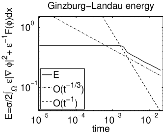
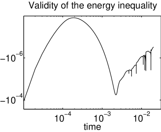
Figure 1: Time evolution of the Ginzburg–Landau energy (left), and validity of the energy inequality (right).

The violation in the conservation of mass

Since we use Lagrange interpolation as projection operator between successive grids, we do not have full mass conservation, but have a violation in the mean value of $\varphi$ as discussed in Remark 4. In Figure 2 we depict the time evolution of the term $\left|\int_{\Omega}\varphi^{k+1}-\varphi^{0}\,dx\right|$, i.e. the difference between the mean value of $\varphi$ and the mean value of the initial phase field $\varphi^{0}$. The numerical setup is the spinodal decomposition.

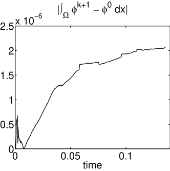
Figure 2: Time evolution of the deviation of the mean value of $\varphi$.

As can be observed, the violation increases with time, and the violation in mass conservation finally is of size $10^{-6}$. We note that the order of the mean value is $|\Omega|$ and here we have $|\Omega|=1$. Thus though we have deviation of mass, its size is small in comparison to the actual mean value.

Comparison with an existing benchmark

In [HTK⁺09] a quantitative benchmark for the simulation of the rising bubble is proposed. Three different groups provided numerical results for two benchmark computations of rising bubble scenarios, using sharp interface models. In [AV12] the [HTK⁺09] benchmark is implemented with computations based on three different diffuse interface approximations to the setup of [HTK⁺09].

We briefly describe the setup. We start with an inital bubble of radius $r=0.25$ located at $M=(0.5,0.5)$ with physical surface tension $\sigma^{phys}=24.5$, resulting in $\sigma\approx 15.5972$ (see [AGG12, Sec. 4.3.4]). The initial velocity is zero. In the domain $\Omega=(0,1)\times(0,2)$ we have no-slip boundary conditions for the velocity field on top and bottom walls, and free-slip on the left and the right walls. The parameters are given as $\rho_{1}=1000$, $\rho_{2}=100$, $\eta_{1}=10$, $\eta_{2}=1$, resulting in a Reynolds number of 35. Here $\rho_{2}$ and $\eta_{2}$ correspond to the fluid in the bubble. Due to the smaller density we expect the bubble to rise in the gravity field with force $g=(0,-0.98)^{t}$. Since we use a diffuse interface model, we have the additional parameters $m\equiv 10^{-3}\epsilon$ and $\epsilon=0.02$. The time discretization step is chosen as $\tau=2.5e-5$. The rising bubble is simulated over a time horizon of $3$ units of time.

In [HTK⁺09] the following benchmark parameters are defined. For a bubble represented by $\varphi(x)<0$ we measure the evolution of circularity, rising velocity and of the center of mass.

The circularity is defined by

$$\Theta_{\varphi}=\frac{\mbox{perimeter\,of\,area-equivalent\,circle}}{\mbox{perimeter\,of\,bubble}}\leq 1,$$

the rising velocity is defined as

$$V_{\varphi}=\frac{\int_{\varphi<0}v\,dx}{\int_{\varphi<0}1\,dx},$$

and the center of mass is given by

$$M_{\varphi}=\frac{\int_{\varphi<0}x_{2}\,dx}{\int_{\varphi<0}1\,dx}.$$

Here $x_{2}$ denotes the second component of the spatial variable $x=(x_{1},x_{2})$. Note that the process is symmetric and it is sufficient to integrate over the second component.

As benchmark values the minimal circularity $(\Theta_{\varphi})_{\min}$ together with the time $t_{\Theta}:=t(\Theta_{\varphi}\equiv(\Theta_{\varphi})_{\min})$, the maximal rising velocity $(V_{\varphi})_{\max}$ together with the time $t_{V}:=t(V_{\varphi}\equiv(V_{\varphi})_{\max})$ and the center of mass $M_{\varphi}(t=3)$ at the final time $t=3$ are presented.

Our results are shown in Table 1, first row (GHK $\epsilon=0.02$). For comparison we in the second row also give the results obtained in [AV12] (AV $\epsilon=0.02$). Note that there the polynomial double well free energy is used resulting in a diffuser interface. The results in the following rows are taken from the sharp interface numerics in [HTK⁺09]. The groups TP2D, FreeLIFE and MooNMD are the groups participating in [HTK⁺09]. The group TP2D is the group of Turek at the Technical University of Dortmund, FreeLIFE is provided by the École polytechnique fédérale de Lausanne by the group of Burman and MooNMD is the group of Tobiska from the University of Magdeburg. With BGN we denote the results presented in [BGN13], which are obtained by a sharp interface approach based on the model used in the present paper.

Group	$(\Theta_{\varphi})_{\min}$	$t_{\Theta}$	$(V_{\varphi})_{\max}$	$t_{V}$	$M_{\varphi}(t=3)$
GHK $\epsilon=0.02$	0.9080	1.9672	0.2388	0.9765	1.0786
AV $\epsilon=0.02$	0.9159	2.0040	0.2375	1.0400	1.0733
TP2D	0.9013	1.9041	0.2417	0.9213	1.0813
FreeLIFE	0.9011	1.8750	0.2421	0.9313	1.0799
MooNMD	0.9013	1.9000	0.2417	0.9239	1.0817
BGN	0.9014	1.9000	0.2417	0.9230	1.0819

Table 1: Results for the first benchmark from [HTK⁺09].

We see that our results are in quite good aggrement with those obtained with sharp interface numerics.

In Figure 3 we show the evolution of the bubble for the benchmark setting.

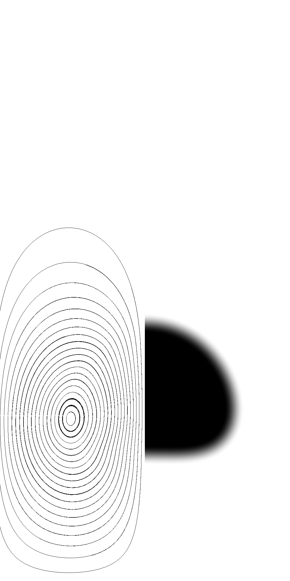
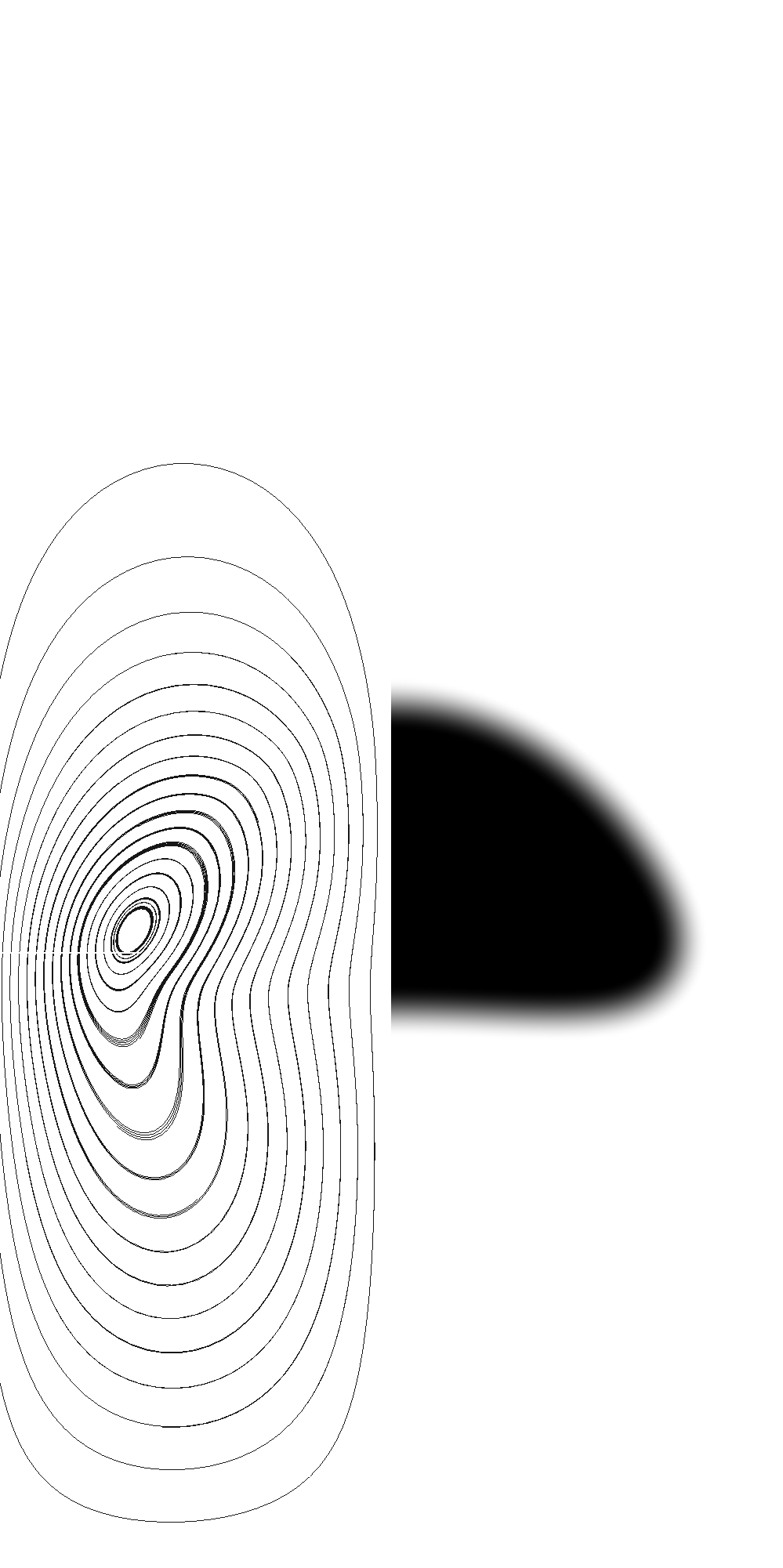
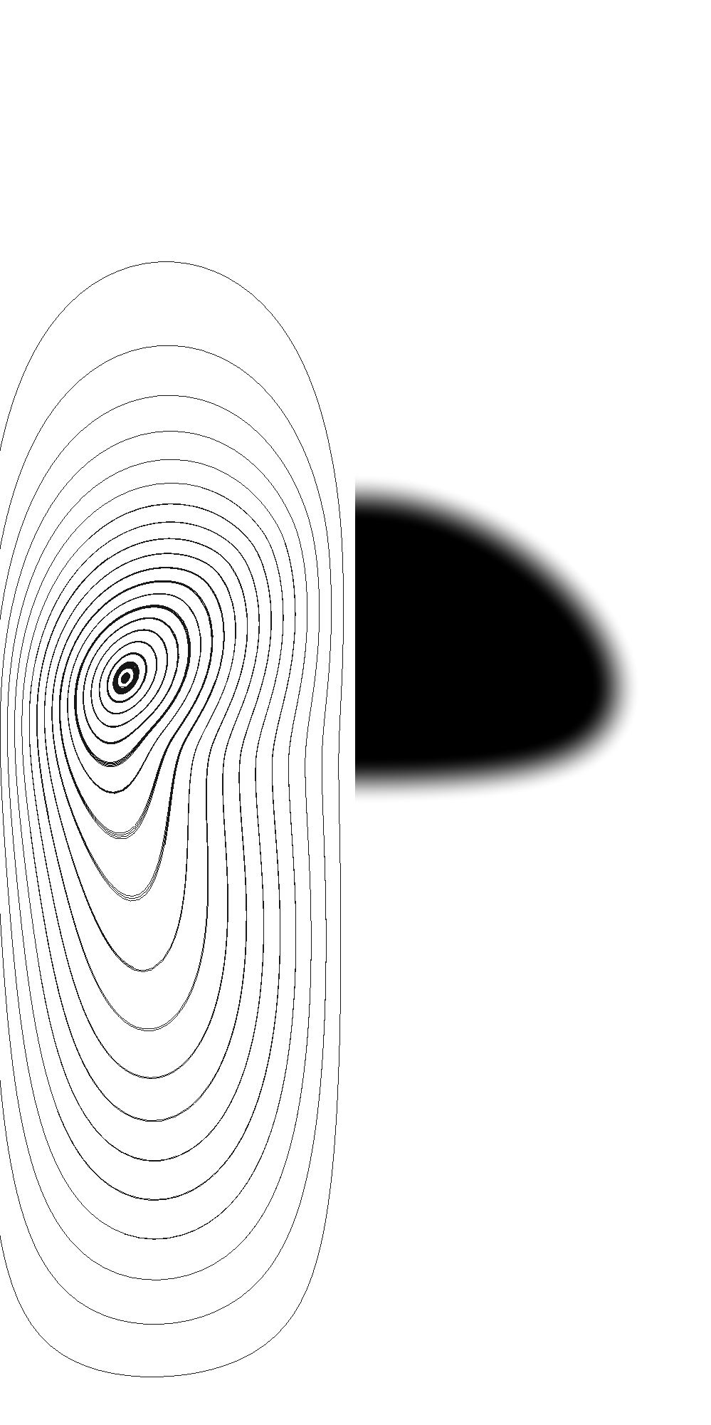
Figure 3: The evolution of the bubble at times $t\in\{0,1,2,3\}$. The phase field is shown in the right part and streamlines of the velocity field in the left part of each plot.

Distribution of the error indicators

Next we investigate the distribution of the error indicators. We observe that a similar distribution is observed as in the case of the numerical simulation of the Cahn–Hilliard equation with transport reported in [HHK13]. The errors are concentrated at the boundary of the interface. We further have additional error contributions from the Navier–Stokes part in a neighborhood of the bubble.

In Figure 5 we show the distribution of the error indicators $\eta_{T}$ and $\eta_{TE}$ defined in Algorithm 1.

Figure 4: The distribution of the error indicators at time $t=3$. $\eta_{T}$ on the left, $\eta_{TE}$ on the right. Black indicates higher errors.

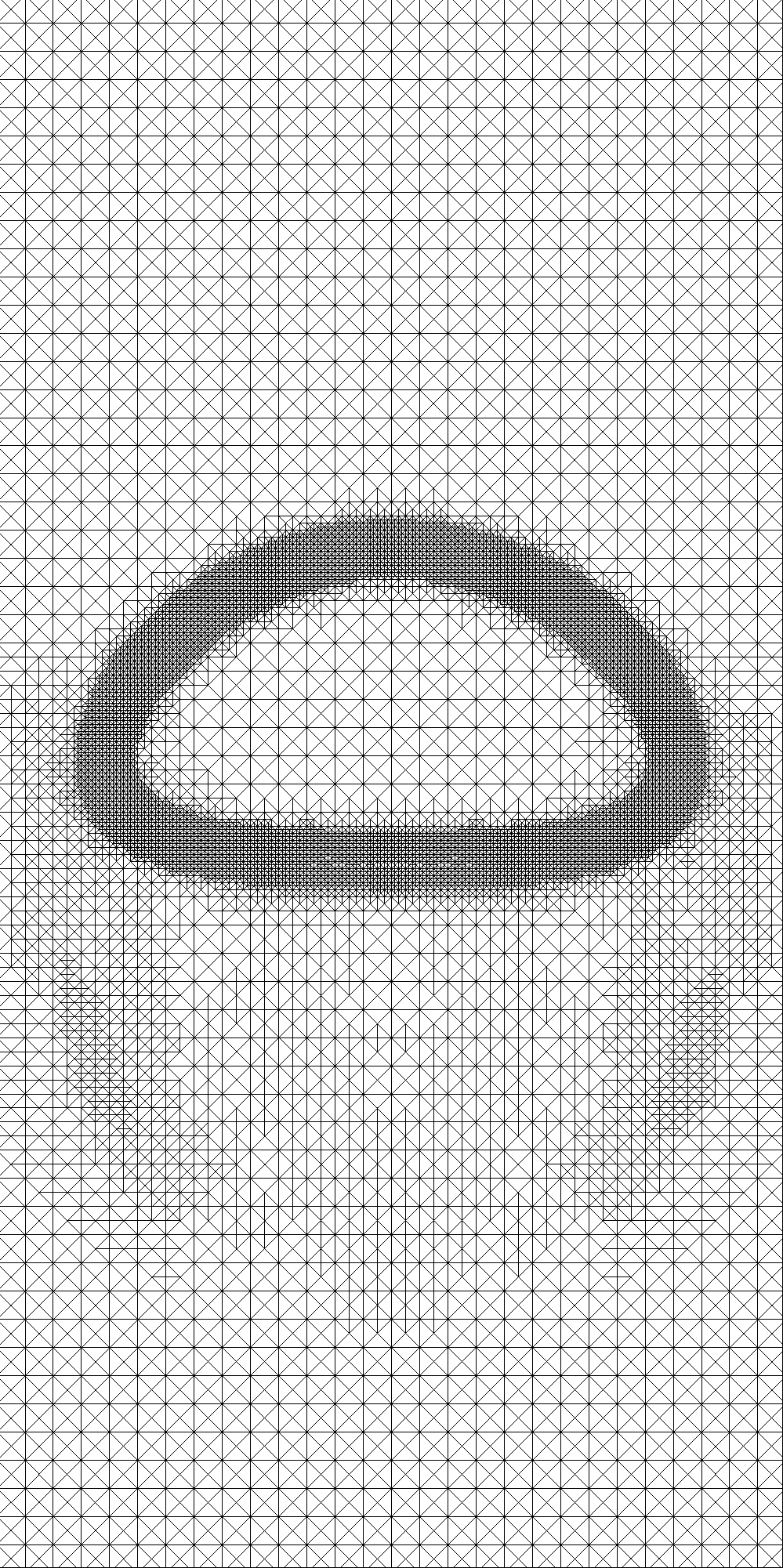
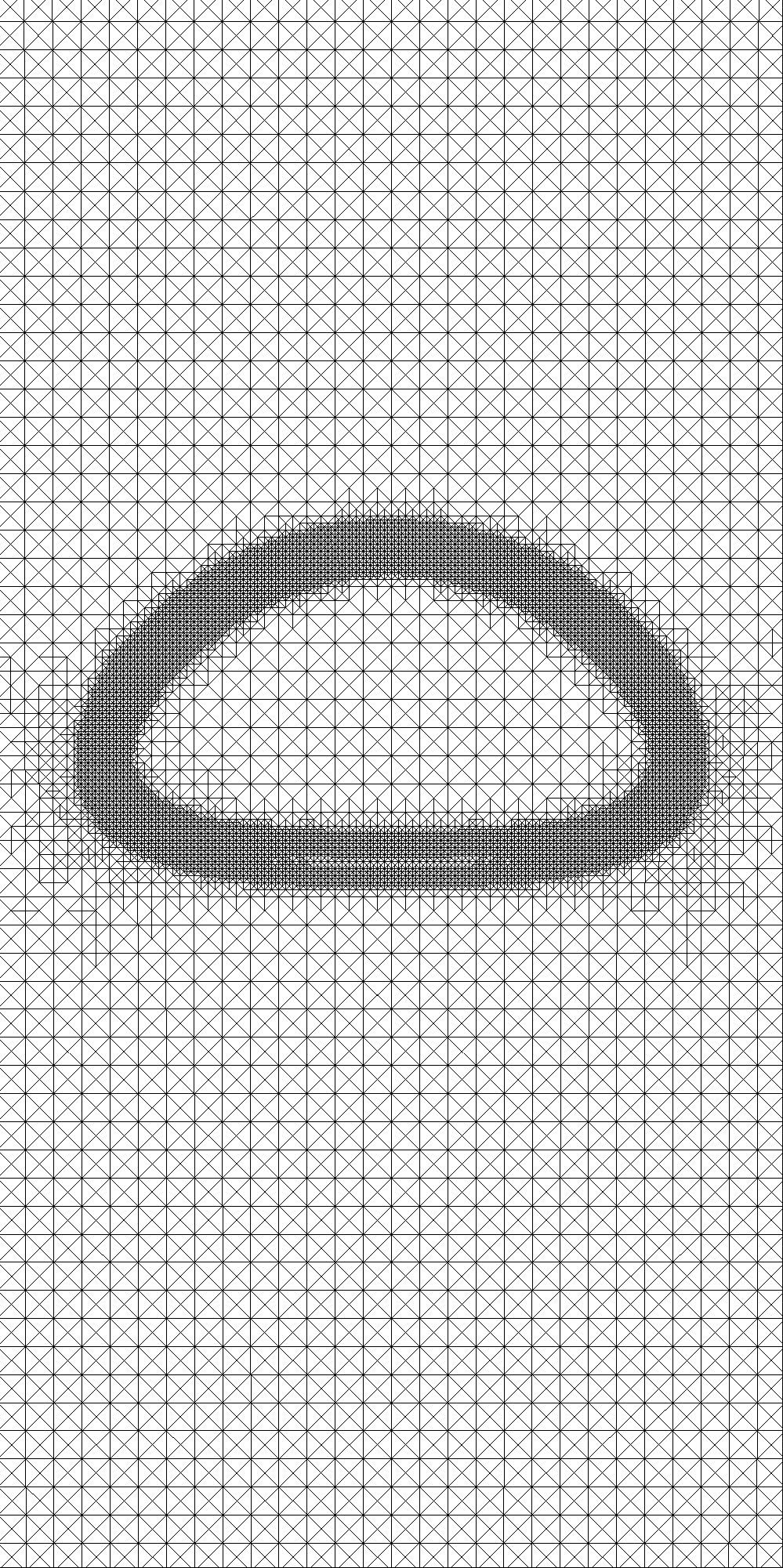
Figure 5: The mesh with (left) and without (right) postprocessing at final time $t=3$.

Influence of the post processing of the marked triangles

Finally we investigate the spatial discretization obtained by our adaptive concept. Especially we show the influence of the post processing step of Algorithm 2 on reducing the number of triangles that are coarsened.

We simulate the rising bubble benchmark in the setting described above with and without the postprocessing steps. We note that without the postprocessing artificial energy is generated numerically through the coarsening process and the validity of the energy inequality can not be guaranteed, and in fact is not given.

In Figure 5 we show the final meshes at $t=3$ with postprocessing (left) and without postprocessing (right). We see that there are regions in the bulk phase below the bubble where the postprocessing prevents the adaptive strategy from coarsening the triangles to the coarsest level. Thus we obtain a larger number of nodes if we use the post processing as is demonstrated in Figure 6 where we display the evolution of the number of mesh nodes with and without postprocessing.

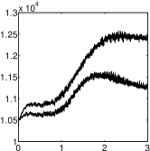
Figure 6: The evolution of the number of nodes for the described benchmark with (upper line) and without (lower line) postprocessing.

We see that the number of nodes increases (by maximal 10% in this example) since not all triangles that are marked for coarsening are coarsened. On the other hand we note, that the energy inequality in the case without post processing is violated in 1692 of 60000 simulation steps and this violation takes place within the first 7000 time steps.

Let us note, that from the fluid mechanical point of view and if one considers the bubble as an obstacle in the channel flow, the region detected by the post processing is the wake, where the fluid is accelerated. Thus we expect a refined flow mesh there.

5 Conclusion

We propose a time discretization for the thermodynamically consistent model from [AGG12] that gives rise to a time discrete energy inequality that can be conserved in the fully discrete setting. The systems to be solved in the discrete setting are fully coupled and a concept for handling the linear systems arising from Newton’s method is proposed.

Based on the energy inequality we derive an error estimator both measuring the local error in the discretization of the velocity field, and in the phase field and the chemical potential. We investigate the behavior of our solver and especially could numerically verify the validity of the discrete energy inequality.

Post processing, applied to fulfill the energy inequality in the discrete setting, in our example leads to meshes containing approximatly 10% more triangles than the meshes obtained without post processing, but to a more reasonable refinement from the flow-physics point of view. The numerical results might be further improved by replacing the Lagrange interpolation operator by e.g. the mass-conserving quasi-interpolation operator introduced in [Car99]. This will be subject to future work.

References

• [ADG13a] H. Abels, D. Depner, and H. Garcke. Existence of weak solutions for a diffuse interface model for two-phase flows of incompressible fluids with different densities. Journal of Mathematical Fluid Mechanics, 15(3):453–480, September 2013.
• [ADG13b] H. Abels, D. Depner, and H. Garcke. On an incompressible Navier–Stokes / Cahn–Hilliard system with degenerate mobility. Annales de l’Institut Henri Poincaré (C) Non Linear Analysis, 30(6):1175–1190, 2013.
• [ADGK13] G. L. Aki, W. Dreyer, J. Giesselmann, and C. Kraus. A quasi-incompressible diffuse interface model with phase transition. Mathematical Models and Methods in Applied Sciences (online ready), 2013.
• [AF03] R. A. Adams and J. H. F. Fournier. Sobolov Spaces, second edition, volume 140 of Pure and Applied Mathematics. Elsevier, 2003.
• [AGG12] H. Abels, H. Garcke, and G. Grün. Thermodynamically consistent, frame indifferent diffuse interface models for incompressible two-phase flows with different densities. Mathematical Models and Methods in Applied Sciences, 22(3):40, March 2012.
• [AMW98] D. M. Anderson, G. B. McFadden, and A. A. Wheeler. Diffuse-interface methods in fluid mechanics. Annual Review of Fluid Mechanics, 30:139–165, 1998.
• [AO00] M. Ainsworth and J. T. Oden. A Posteriori Error Estimation in Finite Element Analysis. Wiley, September 2000.
• [AV12] S. Aland and A. Voigt. Benchmark computations of diffuse interface models for two-dimensional bubble dynamics. International Journal for Numerical Methods in Fluids, 69:747–761, 2012.
• [BBG11] L. Blank, M. Butz, and H. Garcke. Solving the Cahn–Hilliard variational inequality with a semi-smooth Newton method. ESAIM: Control, Optimisation and Calculus of Variations, 17(4):931–954, Oktober 2011.
• [BE91] J. F. Blowey and C. M. Elliott. The Cahn–Hilliard gradient theory for phase separation with non-smooth free energy. Part I: Mathematical analysis. European Journal of Applied Mathematics, 2:233–280, 1991.
• [BGN13] J. W. Barrett, H. Garcke, and R. Nürnberg. A Stable Parametric Finite Element Discretization of Two-Phase Navier–Stokes Flow. preprint in arXiv: 1308.3335, 2013.
• [BN09] L. Baňas and R. Nürnberg. A posteriori estimates for the Cahn–Hilliard equation. Mathematical Modelling and Numerical Analysis, 43(5):1003–1026, September 2009.
• [Boy02] F. Boyer. A theoretical and numerical model for the study of incompressible mixture flows. Computers & Fluids, 31(1):41–68, January 2002.
• [BP88] J. H. Bramble and J. E. Pasciak. A preconditioning technique for indefinite systems resulting from mixed approximations of elliptic problems. Mathematics and Computation, 50(181):1–17, 1988.
• [Car99] C. Carstensen. Quasi-interpolation and a-posteriori error analysis in finite element methods. Mathematical Modelling and Numerical Analysis, 33(6):1187–1202, 1999.
• [CDHR08] Y. Chen, T. A. Davis, W. W. Hager, and S. Rajamanickam. Algorithm 887: Cholmod, supernodal sparse cholesky factorization and update/downdate. ACM Transactions on Mathematical Software, 35(3):1–14, 2008.
• [CF88] P. Constantin and C. Foias. Navier-Stokes-Equations. The University of Chicago Press, 1988.
• [CH58] J. W. Cahn and J. E. Hilliard. Free Energy of a Nonuniform System. I. Interfacial Free Energy. The Journal of Chemical Physics, 28(2):258–267, 1958.
• [Che08] L. Chen. $i$FEM: An Innovative Finite Element Method Package in Matlab, available at: ifem.wordpress.com, 2008.
• [Clé75] P. Clément. Approximation by finite element functions using local regularization. RAIRO Analyse numérique, 9(2):77–84, August 1975.
• [Dav04] T. A. Davis. Algorithm 832: Umfpack v4.3 - an unsymmetric-pattern multifrontal method. ACM Transactions on Mathematical Software, 30(2):196–199, 2004.
• [DSS07] H. Ding, P. D. M. Spelt, and C. Shu. Diffuse interface model for incompressible two-phase flows with large density ratios. Journal of Computational Physics, 226(2):2078–2095, October 2007.
• [EG04] A. Ern and J.-L. Guermond. Theory and practice of finite elements, volume 159 of Applied mathematical sciences. Springer Verlag, New York, 2004.
• [Fen06] X. Feng. Fully Discrete Finite Element Approximations of the Navier–Stokes–Cahn–Hilliard Diffuse Interface Model for Two-Phase Fluid Flows. SIAM Journal on Numerical Analysis, 44(3):1049–1072, 2006.
• [FM08] E. P. Favvas and A. C. Mitropoulos. What is spinodal decomposition? Journal of Engineering Science and Technology Review, 1:25–27, 2008.
• [GK14] G. Grün and F. Klingbeil. Two-phase flow with mass density contrast: Stable schemes for a thermodynamic consistent and frame indifferent diffuse interface model. Journal of Computational Physics, 257(A):708–725, January 2014.
• [GLL] Z. Guo, P. Lin, and J. S. Lowengrub. A numerical method for the quasi-incompressible Cahn–Hilliard–Navier–Stokes equations for variable density flows with a discrete energy law. preprint in arXiv: 1402.1402.
• [GR86] V. Girault and P. A. Raviart. Finite Element Methods for Navier–Stokes Equations, volume 5 of Springer series in computational mathematics. Springer, 1986.
• [Grü13] G. Grün. On convergent schemes for diffuse interface models for two-phase flow of incompressible fluids with general mass densities. SIAM Journal on Numerical Analysis, 51(6):3036–3061, 2013.
• [HHK13] M. Hintermüller, M. Hinze, and C. Kahle. An adaptive finite element Moreau–Yosida-based solver for a coupled Cahn–Hilliard/Navier–Stokes system. Journal of Computational Physics, 235:810–827, February 2013.
• [HHT11] M. Hintermüller, M. Hinze, and M. H. Tber. An adaptive finite element Moreau–Yosida-based solver for a non-smooth Cahn–Hilliard problem. Optimization Methods and Software, 25(4-5):777–811, 2011.
• [HIK03] M. Hintermüller, K. Ito, and K. Kunisch. The primal-dual active set strategy as a semi-smooth Newton method. SIAM Journal on Optimization, 13(3):865–888, 2003.
• [HTK+09] S. Hysing, S. Turek, D. Kuzmin, N. Parolini, E. Burman, S. Ganesan, and L. Tobiska. Quantitative benchmark computations of two-dimensional bubble dynamics. International Journal for Numerical Methods in Fluids, 60(11):1259–1288, 2009.
• [KLW02] D. Kay, D. Loghin, and A. Wathen. A preconditioner for the steady state Navier–Stokes equations. SIAM Journal on Scientific Computing, 24(1):237–256, 2002.
• [KSW08] D. Kay, V. Styles, and R. Welford. Finite element approximation of a Cahn–Hilliard–Navier–Stokes system. Interfaces and Free Boundaries, 10(1):15–43, 2008.
• [LT98] J. Lowengrub and L. Truskinovsky. Quasi-incompressible Cahn–Hilliard fluids and topological transitions. Proceedings of the royal society A, 454(1978):2617–2654, 1998.
• [OSS13] F. Otto, C. Seis, and D. Slepčev. Crossover of the coarsening rates in demixing of binary viscous liquids. Communications in Mathematical Sciences, 11(2):441–464, 2013.
• [Sig79] E. D. Siggia. Late stages of spinodal decomposition in binary mixtures. Physical Review A, 29(2):595–605, August 1979.
• [Tem77] R. Temam. Navier–Stokes equations - Theory and numerical analysis. North-Holland Publishing Company, 1977.
• [Ver10] R. Verfürth. A posteriori error analysis of space-time finite element discretizations of the time-dependent Stokes equations. Calcolo, 47:149–167, 2010.