Perturbation solutions of the
semiclassical Wigner equation

Abstract

We present a perturbation analysis of the semiclassical Wigner equation which is based on the interplay between configuration and phase spaces via Wigner transform. We employ the so-called harmonic approximation of the Schrödinger eigenfunctions for single-well potentials in configuration space, to construct an asymptotic expansion of the solution of the Wigner equation. This expansion is a perturbation of the Wigner function of a harmonic oscillator but it is not a genuine semiclassical expansion because the correctors depend on the semiclassical parameter. However, it suggests the selection of a novel ansatz for the solution of the Wigner equation, which leads to an efficient regular perturbation scheme in phase space. The validity of the approximation is proved for particular classes of initial data. The proposed ansatz is applied for computing the energy density of a a quartic oscillator on caustics (focal points). The results are compared with those derived from the so-called classical approximation whose principal term is the solution of Liouville equation with the same initial data. It turns out that the results are in good approximation when the coupling constant of the anharmonic potential has certain dependence on the semiclassical parameter.

1 Introduction

WKB solutions and geometrical optics.

We consider the oscillatory initial value problem

$$\left\{\begin{array}[]{l}i\varepsilon\frac{{\partial\psi^{\varepsilon}}}{{\partial t}}=\widehat{H}\psi^{\varepsilon}(x,t),\ \ x\in\mathbb{R},\ t>0\\ \psi^{\varepsilon}(x,0)=\psi^{\varepsilon}_{0}(x)\ ,\ \ \varepsilon<<1\ ,\end{array}\right.$$ (1.1)

where $\widehat{H}=-\frac{\varepsilon^{2}}{2}\partial^{2}_{x}+V(x)$ is the usual quantum mechanical Schrödinger operator. High frequency waves that satisfy (1.1) with oscillatory initial data

$$\psi^{\varepsilon}_{0}(x)=A_{0}(x)\exp(iS_{0}(x)/\varepsilon)\ ,$$ (1.2)

have been traditionally studied by geometrical optics. This method departs from the construction of WKB approximate solutions in the form ([3], [7], [25])

$$\psi^{\varepsilon}(x,t)=A(x,t)\exp(iS(x,t)/\varepsilon)\ ,$$ (1.3)

where the phase function $S(x,t)$ and the amplitude $A(x,t)$ are usually assumed to be real-valued functions, although extensions of the method for complex-valued phases have been also developed.

Substituting (1.3) into (1.1), and retaining terms of order $O(\varepsilon)$ and $O(1)$ with respect to $\varepsilon$, we obtain the Hamilton-Jacobi equation for the phase

$$\partial_{t}S+(\partial_{x}S)^{2}/2+V=0\ ,\ \ \ \ S(x,t=0)=S_{0}(x)\ ,$$ (1.4)

and the transport equation for the amplitude

$$\partial_{t}(A^{2})+\partial_{x}\left(A^{2}\partial_{x}S\right)=0\ ,\ \ \ \ A(x,t=0)=A_{0}(x)\ .$$ (1.5)

The system (1.4)-(1.5) is integrated byreduction to a system of ordinary differential equations along bicharacteristics as follows. We define the Hamiltonian function

$$H(x,k)=k^{2}/2+V(x)\ ,$$

and construct the characteristics $(\tilde{x}(t;q),\tilde{k}(t;q))$, as the trajectories of the Hamiltonian system

$$\frac{d\tilde{x}}{dt}=H_{k}(\tilde{x},\tilde{k})=\tilde{k}\ ,\ \ \ \ \ \frac{d\tilde{k}}{dt}=-H_{x}(\tilde{x},\tilde{k})=V^{\prime}(\tilde{x})$$ (1.6)

with initial conditions

$$\tilde{x}(t=0;q)=q\ ,\ \ \ \ \ \ \tilde{k}(t=0;q)=S^{\prime}_{0}(q)\$$

The projection of the characteristics $\tilde{x}=\tilde{x}(t;q)$ on the configuration space are the physical rays of geometrical optics. Then, the phase function $S$ is obtained by integration of the ordinary differential equation

$$\frac{dS}{dt}=\partial_{t}S+\partial_{x}S\frac{dx}{dt}=-H(\tilde{x}(t;q),\tilde{k}(t;q))+\tilde{k}^{2}(t;q)/2=\tilde{k}^{2}(t;q)-V(\tilde{x}(t;q))\ ,$$

with the initial condition

$$S(\tilde{x}(t=0;q))=S_{0}(q)\ .$$

Furthermore, the amplitude $A$ is calculated by applying the divergence theorem in a ray tube, and is given by

$$A(\tilde{x}(t;q),t)=\frac{A_{0}(q)}{\sqrt{J(t;q)}}\ ,$$

where

$$J(t;q)=\frac{\partial\tilde{x}(t;q)}{\partial q}$$

is the Jacobian of the ray transformation $q\mapsto\tilde{x}(t;q)$.

The nonlinear Hamilton-Jacob equation has, in general, multivalued solutions. This means that singularities may be formatted in finite time, when the Jacobian of the ray transformation vanishes. The set $\mathcal{C}=\{x=\tilde{x}(t;q):J(t;q)=0\}$ of these singularities is the caustic of the ray field. On the caustics the amplitude becomes infinite. Therefore, near such singularities the WKB method fails to predict the correct wave field. in the sense that the method cannot describe the correct scales. These scales are predicted either from analytical solutions of model problems, or from uniform asymptotic expansions for the solution of the Schrödinger equation. Such solutions show that the amplitude of the intensity of the wave field increases with the frequency $\varepsilon^{-1}$, but, for any fixed large frequency, it remains bounded with respect to space variables on the caustics.

Assuming that the multivalued function $S$ is known away from caustics, and using boundary layer techniques and matched asymptotic expansions [3], [4], it has been possible to constructed uniform asymptotic expansions near simple caustics. However these analytical techniques are very complicated since the matching procedure depends on the form of the particular caustic.

A different group of uniform methods valid near caustics, is based on integral representations of the solutions in phase-space. The basic methods in this category are the Maslov’s canonical operator[33]. [34], and the Lagrangian integrals (Kravtsov-Ludwig method [24], [31], [25]), which can be considered as special cases of Fourier integral operators [16], [49].

All the above described techniques assume an ansatz for the solution in the configuration space, which for the final determination requires the knowledge of the multivalued phase functions, or, geometrically, of the Lagrangian manifold generated by the bicharacteristics of the Hamiltonian system in phase space.

An alternative approach is based on the use of the Wigner transform. This is a function defined on phase space as the Fourier transform of the two-point correlation of the wave function. It was introduced by Wigner [52] for specific purposes in quantum thermodynamics, and recently it has been successfully used in semiclassical analysis for the reformulation of wave equations as non local equations in phase space, and the study of of homogenization problems in high-frequency waves [21].

The Wigner equation.

The Wigner transform of a function $f\in L^{2}$, is defined as

$$W^{\varepsilon}[f](x,k)=\frac{1}{2\pi\varepsilon}\int_{\mathbb{R}}e^{-\frac{i}{\varepsilon}k\xi}f(x+\frac{\xi}{2})\overline{f}(x-\frac{\xi}{2})d\xi$$ (1.7)

and for a pair of functions $f,g\in L^{2}(\mathbb{R})$, the (cross) Wigner transform is defined as

$$W^{\varepsilon}[f,g](x,k)=\frac{1}{2\pi\varepsilon}\int_{\mathbb{R}}e^{-\frac{i}{\varepsilon}k\xi}f(x+\frac{\xi}{2})\overline{g}(x-\frac{\xi}{2})d\xi\ .$$ (1.8)

By its definition $W^{\varepsilon}[f](x,k)$ is a real , square integrable, but not necessarily non-negative function in phase space. For this reason it is not a pure probability distribution function, but it is exactly this property that makes the Wigner function a powerful tool in the study of wave and quantum interference phenomena.

Some of the most important relations of Wigner functions

$$W^{\varepsilon}(x,k):=W^{\varepsilon}[\psi^{\varepsilon}](x,k)$$ (1.9)

with the wave function $\psi^{\varepsilon}(x)$ (this in general depends also on time $t$), that are useful for the computation of physical quantities both in classical wave propagation and in quantum mechanics, are the following

1) The integral of $W^{\varepsilon}$ with respect to the momentum $k$ gives the energy density

$$\eta^{\varepsilon}(x):=|\psi^{\varepsilon}(x)|^{2}=\int_{\mathbb{R}}W^{\varepsilon}(x,k)dk\ ,$$ (1.10)

while the first moment with respect to the momentum gives the energy flux,

$$\mathcal{F^{\varepsilon}}(x):=\frac{\varepsilon}{2i}\Bigl{(}\overline{\psi}^{\varepsilon}\partial_{x}\psi^{\varepsilon}-\psi^{\varepsilon}\partial_{x}\overline{\psi}^{\varepsilon}\Bigr{)}=\int_{\mathbb{R}}kW^{\varepsilon}(x,k)dk$$ (1.11)

and its integral over the whole phase space, gives the total energy

$$\int_{\mathbb{R}}\int_{\mathbb{R}}dxdkW^{\varepsilon}(x,k)=\|\psi^{\varepsilon}\|_{L^{2}}\ .$$ (1.12)

2) The Wigner transform of a WKB function

$$\psi^{\varepsilon}(x)=A(x)\exp(iS(x)/\varepsilon)\ ,$$

considered as a generalized function, as $\varepsilon\rightarrow 0$, has the weak limit

$$W^{\varepsilon}[\psi^{\varepsilon}](x,k)\rightharpoonup|A(x)|^{2}\delta\bigl{(}k-S^{\prime}(x)\bigr{)}\ ,$$ (1.13)

where $\delta$ denotes the Dirac distribution [30], [38].

The evolution equation of the Wigner function $W^{\varepsilon}(x,k,t):=W^{\varepsilon}[\psi^{\varepsilon}](x,k,t)$ corresponding to the solution $\psi^{\varepsilon}(x,t)$ of (1.1) has the form

$$\left\{\begin{array}[]{l}\frac{\partial}{\partial t}W^{\varepsilon}(x,k,t)+\mathcal{L}^{\varepsilon}W^{\varepsilon}(x,k,t)=0,(x,k)\in\mathbb{R}^{2},t>0\\ W^{\varepsilon}(x,k,t)|_{t=0}=W^{\varepsilon}_{0}(x,k)\end{array}\right.$$ (1.14)

where $W^{\varepsilon}_{0}(x,k)$ is the Wigner transform of the initial data $\psi^{\varepsilon}_{0}(x)$. and $\mathcal{L}^{\varepsilon}$ is the pseudo differential operator defined by ([5], [17])

$$\mathcal{L}^{\varepsilon}\cdot:=-\frac{2}{\varepsilon}\sin\Bigl{(}\frac{\varepsilon}{2}\Lambda\Bigr{)}H(x,k)\cdot$$ (1.15)

For a general Hamiltonian $H(x,k)$ the operator $\Lambda$ is the commutator

$$\Lambda:=\frac{\partial}{\partial x_{H}}\frac{\partial}{\partial k}-\frac{\partial}{\partial x}\frac{\partial}{\partial k_{H}}\ ,$$

and $\sin\Bigl{(}\frac{\varepsilon}{2}\Lambda\Bigr{)}$ acts on the product of two functions $f(x,k)$ and $g(x,k)$ by the formula

$$\sin\Bigl{(}\frac{\varepsilon}{2}\Lambda\Bigr{)}f(x,k)g(x,k)=$$

$$=\frac{1}{2i\pi^{2}\varepsilon^{2}}\int dk^{\prime}dk^{\prime\prime}dx^{\prime}dx^{\prime\prime}\left[f(x^{\prime},k^{\prime})g(x^{\prime\prime},k^{\prime\prime})-g(x^{\prime},k^{\prime})f(x^{\prime\prime},k^{\prime\prime})\right]$$

$$\times\exp\left(-\frac{2i}{\varepsilon}\left(k(x^{\prime}-x^{\prime\prime})+k^{\prime}(x^{\prime\prime}-x)+k^{\prime\prime}(x-x^{\prime})\right)\right)\ .$$

We also introduce for later use (see eq (2.3) in Section 2) the pseudo-differential operator

$$\mathcal{M}^{\varepsilon}\cdot:=\cos\Bigl{(}\frac{\varepsilon}{2}\Lambda\Bigr{)}H(x,k)\cdot$$ (1.16)

which is known in physics’ literature as Baker’s cosine bracket, by ([13], [17], [48]), and $\cos\Bigl{(}\frac{\varepsilon}{2}\Lambda\Bigr{)}$ acts on the product of two functions $f(x,k)$ and $g(x,k)$ as follows

$$\cos\Bigl{(}\frac{\varepsilon}{2}\Lambda\Bigr{)}f(x,k)g(x,k)=$$

$$=\frac{1}{2\pi^{2}\varepsilon^{2}}\int dk^{\prime}dk^{\prime\prime}dx^{\prime}dx^{\prime\prime}\left[f(x^{\prime},k^{\prime})g(x^{\prime\prime},k^{\prime\prime})+g(x^{\prime},k^{\prime})f(x^{\prime\prime},k^{\prime\prime})\right]$$

$$\times\exp\left(-\frac{2i}{\varepsilon}\left(k(x^{\prime}-x^{\prime\prime})+k^{\prime}(x^{\prime\prime}-x)+k^{\prime\prime}(x-x^{\prime})\right)\right)\ .$$

In the particular case of the usual quantum mechanical Hamiltonian $H(x,k)=k^{2}/2+V(x)$, by using (1.15), the operator $\mathcal{L}^{\varepsilon}$ may also be written in the more standard form

$$\mathcal{L}^{\varepsilon}=k\partial_{x}-\Theta^{\varepsilon}[V]$$ (1.17)

where the operator $\Theta^{\varepsilon}[V]$ is expresses as the convolution

$$\Theta^{\varepsilon}[V]W^{\varepsilon}(x,k,t):=Z^{\varepsilon}(x,k)*_{k}W^{\varepsilon}(x,k,t)\ ,$$ (1.18)

of the Wigner function with the kernel

$$Z^{\varepsilon}(x,k)=\frac{1}{i\varepsilon}\frac{1}{2\pi}\int_{\mathbb{R}}e^{-iky}\left(V(x+\frac{\varepsilon}{2}y)-V(x-\frac{\varepsilon}{2}y)\right)dy\ .$$ (1.19)

This is a non-local operator which the action of the potential on the evolution of Wigner function.

From and(1.18) (1.19) we can write the action of $\Theta^{\varepsilon}[V]$ as a pseudo-differential operator

$$\Theta^{\varepsilon}[V]W^{\varepsilon}(x,k,t)=\frac{i}{2\pi\varepsilon}\int_{\mathbb{R}}\int_{\mathbb{R}}e^{i(k-\xi)y}W^{\varepsilon}(x,\xi,t)\left[V(x+\frac{\varepsilon}{2}y)-V(x-\frac{\varepsilon}{2}y)\right]dyd\xi\ .$$ (1.20)

Now we observe that if the potential function $V$ is smooth enough, using its Taylor expansion we may rewrite quantum Liouville or Wigner operator $\mathcal{L}^{\varepsilon}$ in the form of an infinite order differential operator

$$\mathcal{L}^{\varepsilon}=k\frac{\partial}{\partial x}-V^{\prime}(x)\frac{\partial}{\partial k}-\sum_{j=1}^{\infty}\varepsilon^{2j}\left(\frac{i}{2}\right)^{2j}\frac{V^{(2j+1)}(x)}{(2j+1)!}\frac{\partial^{(2j+1)}}{\partial k^{2j+1}}\ .$$ (1.21)

Thus the Wigner equation (1.14) is written in the form of an infinite order ingular perturbation equation

$$\partial_{t}W^{\varepsilon}+k\partial_{x}W^{\varepsilon}-V^{\prime}(x)\partial_{k}W^{\varepsilon}=\sum_{m=1}^{\infty}\alpha_{m}\varepsilon^{2m}V^{(2m+1)}(x)\partial_{k}^{2m+1}W^{\varepsilon}(x,k,t)\ ,$$ (1.22)

where $\alpha_{m}=(-1)^{m}/2^{2m}(2m+1)!,\ \ m=0,1,\dots$, and $V^{(2m+1)}(x)=d^{2m+1}V(x)/dx^{2m+1}$.

The form (1.22) of the Wigner equation shows that that this equation is a combination of the classical transport (Liouville) operator in the left hand side, with a dispersion operator of infinite order in he right hand side. Roughly speaking, this combination suggests that the phase space evolution results from the interaction between the classical transport of the Lagrangian manifold generated by the Hamiltonian and a non-local dispersion of energy from the manifold into the whole phase space. This picture is consistent with the fact that in the classical limit $\varepsilon=0$ the dispersion mechanism disappears. Then, the solution of the Wigner equation converges weakly to the so called Wigner measure [30], which satisfies the Liouville equation of classical mechanics. This solution is an always well-defined semiclassical measure, and in the absence of caustics it completely retrieves the results of the WKB method

However, it has been shown in [19], [20] that in the case of multi-phase optics and caustic formation, the limit Wigner measure, although still well-defined as semiclassical measure on phase space, is not the appropriate tool for the computation of energy densities at a fixed point of configuration space, because; (a) it cannot be expressed as a distribution with respect to the momentum for a fixed space-time point, and thus it cannot be used to compute the amplitude of the wavefunction, on caustics, and (b) it is unable to ”recognise” the correct scales of the wavefield near caustics. It has been also shown in [19] that approximate Airy-type solutions of the Wigner equation can, produce reasonable solutions for multiphase problems, and at least for simple caustics,

Therefore the study of asymptotic solutions of the Wigner equation for small $\varepsilon$ is promising for understanding the structure solutions, and for computing energy densities, in multiphase geometrical optics through integration of the Wigner function.

Several asymptotic solutions of the Wigner equation have been proposed in the recent past. Steinrück [47] and Pulvirenti [39], have constructed distributional asymptotic expansions near the solution of the classical Liouville equation, by expanding the initial data in a distributional series with respect to the small parameter. However, Heller [22] has noted that such expansions are not physically appropriate for studying the evolution of singular initial conditions, and he has proposed a different expansion where the first order term is the solution of a classical Liouville equation with an effective potential. The use of modified characteristics and effective potentials aims to include indirectly some quantum phenomena and it is a popular technique in physics and quantum chemistry for the treatment of the quantum Liouville equations (see, e.g., the review paper [28]). It has led to reasonable numerical results, and, somehow, it can be used as an alternative of quantum hydrodynamics (Bohm equations) and of the technique of Gaussian beams. In the same direction, Narcowich [36] proposed a different expansion near the classical Liouville equation without expanding the initial data with respect to the semiclassical parameter, which allows him to avoid the distributional expansions. In a rather different direction, the uniform Airy type asymptotic approximation of the Wigner function that was proposed by Berry [8], has been used in the works of Filippas & Makrakis [19], [20], to contract novel asymptotic solution of the Wigner equation in the presence of simple caustics.

Outline of the paper.

This paper aims to the understanding of asymptotic solutions of Wigner equation, by adopting a new strategy for the construction of asymptotic expansions, that exploits the interplay between configuration and phase spaces via Wigner teansform. Our approach has been motivated by the general idea of using spectral expansions in the construction of high-frequency solutions, which has been developed in [7], Ch. 4, for Schrödinger equations. Eigenfunction expansions can be considered as ‘exact” solutions of the Cauchy problem (1.1), which in contrary to the WKB solutions, do not face caustic problems. When transferred to the phase space by Wigner transform they give corresponding expansions which are ”exact” solutions of the Wigner equation.

In this respect, our strategy is the following:

(1) We construct the Moyal eigenfunctions of the Wigner equation (Section 2.1) and their asymptotic expansions in terms of the Moyal functions of a harmonic oscillator, which arises from the so-called harmonic approximation of Schrödinger eigenfunctions (Section 2.2). We assume a single well potential $V(x)$, so that the Schrödinger spectrum be purely discrete, and spectral information for the Wigner equation be also available.

(2) We transform the eigenfunction expansion of the Schrödinger equation to the phase space, and we construct the solution of the Wigner equation as a series of phase-space Moyal eigenfunctions (Section 3.1). Then, we construct a formal asymptotic expansion (harmonic expansion) for the solution of Wigner equation using the expansions of Moyal eigenfunction derived in the first step, and finally

(3) We propose an ansatz for the solution of the Wigner equation and we develop a regular-perturbation scheme in phase space, for computing the sought for asymptotic expansion for the solution of the Wigner equation (Section 3.2).

In Section 4 we present the so-called classical expansion, where the solution of the Wigner equation is expressed as a perturbation of the solution of classical Liouville equation.

As an application, in Section 5 we apply the proposed scheme for a quartic (anharmonic) oscillator, and we compute the wave amplitude at the beaks of the cusps generated by the oscillator through integration of the approximate Wigner functions with respect to the momentum. The predictions of the harmonic and the classical expansions agree at the singular points provided that a certain relation between the small semiclassical parameter and the coupling constant of the potential holds.

2 Aproximmation of Moyal eigenfunctions

2.1 The Moyal eigenfunctions in phase space

It is known that, in principle, the spectrum of the quantum Liouville operator can be determined from the spectrum of the corresponding Schrödinger operator $\widehat{H}$ (see, e.g. [32], [46]), and, in general, someone anticipates the formula

$$\sigma(\mathcal{L}^{\varepsilon})=\{\frac{i}{\varepsilon}(E-E^{\prime}),\ \ E,\ E^{\prime}\in\sigma(\widehat{H})\}\ ,$$

to hold. In fact, this relation holds for the discrete spectrum

$$\sigma_{p}(\mathcal{L}^{\varepsilon})=\{\frac{i}{\varepsilon}(E^{\varepsilon}_{n}-E^{\varepsilon}_{m}),\ \ E^{\varepsilon}_{n},E^{\varepsilon}_{m}\in\sigma_{p}(\widehat{H})\}\ \ .$$

A similar formula holds for the point spectrum of the cosine bracket operator $\mathcal{M}^{\varepsilon}$ (eq (1.16) below), that is

$$\sigma_{p}(\mathcal{M}^{\varepsilon})=\{\frac{1}{2}(E^{\varepsilon}_{n}+E^{\varepsilon}_{m}),\ \ E^{\varepsilon}_{n},E^{\varepsilon}_{m}\in\sigma_{p}(\widehat{H})\}\ .$$

However, these formulae are not in general true for the absolutely and singular continuous spectrum. These spectral questions have been studied first by Spohn [46], and later by Antoniou et al [2], who have proved the negative result

$$\sigma_{sc,ac}(\mathcal{L}^{\varepsilon})\neq\{\frac{i}{\varepsilon}(E-E^{\prime}),\ \ E,\ E^{\prime}\in\sigma_{sc,ac}(\widehat{H})\}\ ,$$

where $\sigma_{sc,ac}$ denote the singular and absolutely continuous spectrum respectively.

In order to avoid the complications arising from the continuous spectrum (a;though this pertains to the most interesting cases of scattering problems), we consider operators $\widehat{H}$ with purely discrete spectrum $\sigma(\widehat{H})=\sigma_{p}(\widehat{H})$, therefore $\sigma(\mathcal{L}^{\varepsilon})=\sigma_{p}(\mathcal{L}^{\varepsilon})$ and $\sigma(\mathcal{M}^{\varepsilon})=\sigma_{p}(\mathcal{M}^{\varepsilon}).$ When the potential $V(x)\in L^{1}_{loc}(\mathbb{R})$ is bounded below and $\lim_{|x|\rightarrow\infty}V(x)=\infty$ it is known that $\widehat{H}$ has purely discrete spectrum ( [40], [44]), and therefore the operators $\mathcal{L}^{\varepsilon},\mathcal{M}^{\varepsilon}$ have also purely discrete spectrum. We denote by $E^{\varepsilon}_{n}$ and $u^{\varepsilon}_{n}(x)$ the eigenvalues and the eigenfunctions of $\widehat{H}$, that satisfy $\widehat{H}u^{\varepsilon}_{n}(x)=E^{\varepsilon}_{n}u^{\varepsilon}_{n}(x)\ ,\ \ n=1,2,\dots\ .$ It is known that $u^{\varepsilon}_{n}$ form a complete orthonormal basis in $L^{2}(\mathbb{R})$ .

The Moyal eigenfunctions, were introduced by Moyal [35], for the purposes of a concrete statistical study of quantum mechanics, and they are defined as the cross-Wigner transform (1.8) of the Schrödinger eigenfunctions $u^{\varepsilon}_{n}\ ,u^{\varepsilon}_{m}\ ,\ \ \ n,m=0,1,2,\dots$.

$$\Phi^{\varepsilon}_{nm}(x,k):=W^{\varepsilon}[u^{\varepsilon}_{n},u^{\varepsilon}_{m}](x,k)=\frac{1}{\pi\varepsilon}\int_{\mathbf{R}}e^{-i\frac{2k}{\varepsilon}\sigma}u^{\varepsilon}_{n}(x+\sigma)\overline{u^{\varepsilon}_{m}}(x-\sigma)d\sigma\ .$$ (2.1)

For these functions the following theorem holds [35], [48].

Theorem 1.

Let $\widehat{H}$ has purely discrete spectrum $\{E^{\varepsilon}_{n}\}_{n=0,1,2,\dots}$ with complete orthonormal system of eigenfunctions $\{u^{\varepsilon}_{n}(x)\}_{n=0,1,\dots}$ in $L^{2}(\mathbb{R})$. Then, the functions $\{\Phi^{\varepsilon}_{nm}\}_{n,m=0,1,\dots}$ form a complete orthonormal basis in $L^{2}(\mathbb{R}_{xk}^{2})$, and they are common eigenfunctions of the operators $\mathcal{L}^{\varepsilon}$ and $\mathcal{M}^{\varepsilon}$ with eigenvalues $\lambda_{nm}=\frac{i}{\varepsilon}\left(E^{\varepsilon}_{n}-E^{\varepsilon}_{m}\right)$ and $\mu_{nm}=\frac{1}{2}\left(E^{\varepsilon}_{n}+E^{\varepsilon}_{m}\right)$, respectively.

Therefore, $\Phi^{\varepsilon}_{nm}(x,k)$ satisfy the eigenvalue problems

$$\mathcal{L}^{\varepsilon}\Phi^{\varepsilon}_{nm}(x,k)=\lambda_{nm}\Phi^{\varepsilon}_{nm}(x,k)$$ (2.2)

$$\mathcal{M}^{\varepsilon}\Phi^{\varepsilon}_{nm}(x,k)=\mu_{nm}\Phi^{\varepsilon}_{nm}(x,k)\ ,$$ (2.3)

in phase space $L^{2}(\mathbb{R}_{xk}^{2})$

Remark 1. It is very important to note that for the computation of Moyal functions, directly in phase space, we need both eigenvalue problems, (2.2) and (2.3), as it has been explained in [13], [26]. Moreover, there is no evolution equation in phase space which corresponds to the eigenvalue equation (2.3) and which could be deduced from Schrödinger formulation , as is the case for the quantum Liouville equation. This means that (2.3) cannot result naturally from some initial value problem governing the Wigner function. In order to derive the second eigenvalue equation directly from phase space, Fairlie & Manogue [18] extended the Wigner function by introducing an imaginary time variable $s$, thus constructing a second initial value problem, with time derivative $i\partial_{s}$ and space operator $\mathcal{M}^{\varepsilon}$, for the extended Wigner function. Both the mathematical role and the physical content of this new function are still to be understood.

Remark 2. It is also important to note that it is not possible to compute the limits of the Moyal eigenfunctions $\Phi^{\varepsilon}_{nm}$ as $\varepsilon\to 0$, for any $n,m$ independent of each other, a situation which can be somehow considered as a consequence of the Bohr-Sommerfeld quantisation rule. This situation is a fundamental obstruction for the computation of the limit of the phase-space eigenfunction expansion of the Wigner function the $\varepsilon\to 0$, from which one would expect to obtain an analogous generalised expansion of the solution of the classical Liouville equation. What can be evaluated is the classical limit $\varepsilon\to 0$, when $\ n,m\to\infty$ and $n-m=$ constant. For integrable Hamiltonians, Berry & Balazs [8] [9] have computed the classical limit of Moyal functions $\Phi^{\varepsilon}_{nm}$ in the case $n=m$, which reads as $\Phi^{0}_{nn}(I,\theta)=\delta\left(H(I)-(E^{0}_{n})\right)$, where $H(I)$ is the Hamltonian in action angle variables $(I,\theta)$. In the ”simplest” case of the the harmonic oscillator, Ripamonti [42] and Truman & Zhao [50] have given independent proofs for the classical limit of the corresponding Moyal eigenfunctions $\Phi^{\varepsilon}_{nm}$ for all $n,m=0,1,\dots$, based on the asymptotics of Laguerre polynomials. Finally, a formal computation in [51] shows that the classical limit of Moyal eigenfunctions, in terms of action-angle variables , and for all $n\neq m$, reads as

$$\Phi^{0}_{nm}(I,\theta)=e^{-i\frac{E^{0}_{nm}}{\gamma_{nm}}\theta}\delta\left(H(I)-\frac{1}{2}(E^{0}_{n}+E^{0}_{m})\right)\ .$$

where $E^{0}_{n}=lim_{\varepsilon\rightarrow 0}\frac{E^{\varepsilon}}{\varepsilon}$, $E^{0}_{nm}=E^{0}_{n}-E^{0}_{m}$, and $\gamma_{nm}=H^{\prime}\left(H^{-1}(\frac{1}{2}(E^{0}_{n}+E^{0}_{m}))\right)$. Also from this formal computation becomes evident the necessity of both eigenvalue equations (2.2) and (2.3).

2.2 Harmonic approximation of Moyal eigenfunctions

We proceed now to the construction an asymptotic expansion of the Moyal eiegenfunctions, for small $\varepsilon$, starting from the so-called harmonic approximation of the eigenfunctions of the Schrödinger operator in the configuration space.

It is known that the eigenfunctions and eigenvalues of the Schrödinger operator $\widehat{H}$ can be approximated by the corresponding ones of an appropriate harmonic oscillator, provided that the potential $V(x)$ satisfies the following conditions ([23], [44])

(i) $V\in C^{\infty}(\mathbb{R})$
(ii) $V\geq 0,\textrm{ for some }R>0\mathop{\inf}\limits_{|x|>R}V(x)>0\ ,$
(iii) $V^{\prime}\textrm{ has finite number of zeros }\{x^{(\alpha)}\}_{\alpha=1}^{\kappa}\ ,$
(iv)$\textrm{ for each }x^{(\alpha)}\ \ V^{\prime\prime}(x^{(\alpha)})>0\ ,$
(v) $V\textrm{ polynomially bounded }|V(x)|\leq c(1+|x|^{m})\ .$

For simplicity we consider only the case $\kappa=1$, we adopt the normalization $x^{(1)}=0$ and, without loss of generality, we also assume that $V(0)=0$. Although asymptotics of eigenvalues and eigenfunctions are also available for multiple wells, in order to deal with this case it is necessary to consider detailed information on the decay of the eigenfunctions (see, e.g., [11] and the references therein) and take account of tunnelling effects for the Wigner function which is a rather complicated task [6].

Then, the eigenvalues $E^{\varepsilon}_{n}$ and the eigenfunctions $u^{\varepsilon}_{n}(x),\ n=0,1,\dots\ ,$ have the asymptotic expansions

$$\frac{2}{\varepsilon}E^{\varepsilon}_{n}=e_{n}+\sum\limits_{l=1}^{N}a_{n}^{(l)}\varepsilon^{l}+O\left(\varepsilon^{N+1}\right)\ ,$$ (2.4)

and

$$\varepsilon^{\frac{1}{4}}u^{\varepsilon}_{n}(x)\sim\psi_{n}(\frac{x}{\sqrt{\varepsilon}})+\sum\limits_{l=1}^{\infty}\varepsilon^{\frac{l}{2}}\psi_{n}^{(l)}(\frac{x}{\sqrt{\varepsilon}})\ ,\ \ \psi_{n}^{(l)}\in L^{2}(\mathbb{R}),n=0,1,\dots,\ \ l=1,2,\dots\ ,$$ (2.5)

respectively, where $e_{n}$, $\psi_{n}(x)$ are the eigenvalues and eigenfunctions of the harmonic oscillator $\widehat{H}_{h}:=-\triangle+x^{2}$,

$$\begin{array}[]{l}e_{n}=2n+1,\\ \psi_{n}(x)=(2^{n}n!\sqrt{\pi})^{-\frac{1}{2}}e^{-\frac{x^{2}}{2}}H_{n}(x),\ n=0,1,2,..\end{array}$$ (2.6)

$H_{n}(x)$ being the Hermite polynomials [48]. Hence we refer to the expansions (2.4), (2.5) as the harmonic approximation.

Note that (2.5) is understood in the sense that

$$||[U_{\varepsilon}^{-1}u^{\varepsilon}_{n}-\sum\limits_{l=0}^{N}\varepsilon^{\frac{l}{2}}\psi_{n}^{(l)}||_{L^{2}(\mathbb{R})}=O(\varepsilon^{(N+1)/2})\ .$$ (2.7)

where $U_{\varepsilon}$ is a unitary dilation of $f\in L^{2}(\mathbb{R})$ defined by

$$\left[U_{\varepsilon}f\right](x):=\varepsilon^{-\frac{1}{4}}f\left(\frac{x}{\sqrt{\varepsilon}}\right),\ x\in\mathbb{R},\ .$$

The coefficients $a_{n}^{(l)},\psi_{n}^{(l)},n=0,1,\dots\ ,\ l=1,2,\dots\ ,$ can be computed in closed form by the Rayleigh-Schrödinger perturbation technique [40].

By substituting the asymptotic expansions (2.5) of the eigenfunctions $u^{\varepsilon}_{n}$ into th definition of the Moyal eigenfunctions $\Phi^{\varepsilon}_{nm}(x,k),\ n,m=0,1,\dots$, we get the formal expansions

$$\Phi^{\varepsilon}_{nm}(x,k)\sim\Psi^{\varepsilon}_{nm}(x,k)+\sum\limits_{l=1}^{\infty}\varepsilon^{\frac{l}{2}}Z_{nm}^{\varepsilon,(l)}(x,k)\\$$ (2.8)

The first term of the expansion the Moyal eigenfunction of the harmonic oscillator $V_{h}(x)=x^{2}/2$, that is

$$\Psi^{\varepsilon}_{nm}(x,k):=\frac{1}{\pi\varepsilon}\int_{\mathbf{R}}e^{-i\frac{2k}{\varepsilon}\sigma}\psi^{\varepsilon}_{n}(x+\sigma)\overline{\psi^{\varepsilon}_{m}(x-\sigma)}d\sigma,\ n,m=0,1,2,\dots$$

with $\psi^{\varepsilon}_{n}(x)=\left[U_{\varepsilon}\psi_{n}\right](x)$, and $Z_{nm}^{\varepsilon,(l)}$ given by

$$\begin{array}[]{l}Z_{nm}^{\varepsilon,(l)}(x,k)=[U_{\varepsilon,(xk)}{\widetilde{Z}}_{nm}^{(l)}](x,k)\\ {\widetilde{Z}}_{nm}^{(l)}(\xi,\eta)=\sum\limits_{\mu=0}^{l}W[\psi_{n}^{(\mu)},\psi_{m}^{(l-\mu)}](\xi,\eta)\ .\end{array}$$ (2.9)

Here $W[f,g](x,k)=\frac{1}{\pi}\int_{\mathbb{R}}e^{-i2k\sigma}f(x+\sigma)\overline{g}(x-\sigma)d\sigma$ is the cross-Wigner transform for $\varepsilon=1$, and $U_{\varepsilon,(xk)}$ is a dilation of $f\in L^{2}(\mathbb{R}_{xk}^{2})$ in phase space, which is defined by

$$\left[U_{\varepsilon,(xk)}f\right](x,k):=\varepsilon^{-1}f\left(\frac{x}{\sqrt{\varepsilon}},\frac{k}{\sqrt{\varepsilon}}\right)\ ,\ \ (x,k)\in\mathbb{R}_{xk}^{2}\ ,$$ (2.10)

and it has the property $\|\left[U_{\varepsilon,(xk)}f\right]\|_{L^{2}}=\frac{1}{\sqrt{\varepsilon}}\|f\|_{L^{2}}$. Since the first term of the expansion (2.4) pertains to the harmonic oscillator, we refer to it as the harmonic expansion (or harmonic approximation) of the Moyal eigenfunctins.

For simplifying the formulae, in the sequel we introduce the notation ${\widetilde{f}}(\xi,\eta)=[U^{-1}_{\varepsilon,(xk)}f](\xi,\eta)$.

The asymptotic expansion (2.8) of $\Phi^{\varepsilon}_{nm}(x,k)$ is written in the scaled variables $(\xi,\eta)$ as

$$\left[U^{-1}_{\varepsilon,(xk)}\Phi^{\varepsilon}_{nm}\right](\xi,\eta)\sim\Psi_{nm}(\xi,\eta)+\sum\limits_{l=1}^{\infty}\varepsilon^{\frac{l}{2}}{\widetilde{Z}}_{nm}^{(l)}(\xi,\eta)\\$$ (2.11)

since $\Psi^{\varepsilon}_{nm}(x,k)=[U_{\varepsilon,(xk)}\Psi_{nm}](x,k)$, where $\Psi_{nm}(x,k)$, are the cross-Wigner transform of Hermite functions $\psi_{n}$,

$$\Psi_{nm}(x,k):=\frac{1}{\pi}\int_{\mathbb{R}}e^{-i2k\sigma}\psi_{n}(x+\sigma)\overline{\psi_{m}(x-\sigma)}d\sigma.$$

Furthermore, by substituting the expansion (2.8) into the eigenvalue equations (2.2) and (2.3), and equating the coefficients of same powers of $\varepsilon$ as it is customary in regular perturbation schemes, we expect to obtain a hierarchy of equations for the coefficient functions $Z_{nm}^{\varepsilon,(l)}$. This procedure is quite cumbersome since the operators $\mathcal{L}^{\varepsilon}$ and $\mathcal{M}^{\varepsilon}$ depend also on the parameter $\varepsilon$. The first step is to rescale the eigenvalue problems by using the transform $U_{\varepsilon,(xk)}$ and then we use the properties of the potential to expand appropriately the phase space pseudo-differential operators.

Applying the transform $U_{\varepsilon,(xk)}$ onto the eigenvalue problems (2.2), (2.3), we get ,

$${\widetilde{L}}^{\varepsilon}U^{-1}_{\varepsilon,(xk)}\Phi^{\varepsilon}_{nm}=\frac{i}{\varepsilon}(E^{\varepsilon}_{n}-E^{\varepsilon}_{m})U^{-1}_{\varepsilon,(xk)}\Phi^{\varepsilon}_{nm}$$ (2.12)

and

$${\widetilde{M}}^{\varepsilon}U^{-1}_{\varepsilon,(xk)}\Phi^{\varepsilon}_{nm}(x,k)=\frac{1}{2}(E^{\varepsilon}_{n}+E^{\varepsilon}_{m})U^{-1}_{\varepsilon,(xk)}\Phi^{\varepsilon}_{nm}(x,k)\ .$$ (2.13)

The operators ${\widetilde{L}}^{\varepsilon}$ and ${\widetilde{M}}^{\varepsilon}$ are derived from $\mathcal{L}^{\varepsilon}$ and $\mathcal{M}^{\varepsilon}$ are derived by conjugation with the phase-space dilation

$${\widetilde{L}}^{\varepsilon}:=[U_{\varepsilon,(xk)}]^{-1}\mathcal{L}^{\varepsilon}[U_{\varepsilon,(xk)}]\ ,$$

$${\widetilde{M}}^{\varepsilon}:=[U_{\varepsilon,(xk)}]^{-1}\mathcal{M}^{\varepsilon}[U_{\varepsilon,(xk)}].$$

Note that for smooth potential $V(x)$, we can also use the expansions

$$\mathcal{L}^{\varepsilon}=k\frac{\partial}{\partial x}-V^{\prime}(x)\frac{\partial}{\partial k}-\sum_{j=1}^{\infty}\varepsilon^{2j}\left(\frac{i}{2}\right)^{2j}\frac{V^{(2j+1)}(x)}{(2j+1)!}\frac{\partial^{(2j+1)}}{\partial k^{2j+1}}$$

and

$$\mathcal{M}^{\varepsilon}=-\frac{\varepsilon^{2}}{8}\triangle_{xk}+H(x,k)+\sum_{j=1}^{\infty}\varepsilon^{2j}\left(\frac{i}{2}\right)^{2j}\frac{V^{(2j)}(x)}{(2j)!}\partial^{(2j)}_{k}+\frac{\varepsilon^{2}}{8}\partial^{2}_{k}\ ,$$

to get the corresponding expansions of ${\widetilde{L}}^{\varepsilon}$ and ${\widetilde{M}}^{\varepsilon}$. These read as

$${\widetilde{L}}^{\varepsilon}=L_{h}+(\xi-\frac{1}{\sqrt{\varepsilon}}V^{\prime}(\sqrt{\varepsilon}\xi))\frac{\partial}{\partial{\eta}}-\sum\limits_{j=1}^{\infty}\varepsilon^{j}\left(\frac{i}{2}\right)^{2j}\frac{1}{(2j+1)!}\frac{V^{(2j+1)}(\sqrt{\varepsilon}\xi)}{\sqrt{\varepsilon}}\frac{\partial^{(2j+1)}}{\partial{\eta^{2j+1}}}$$ (2.14)

$$\frac{1}{\varepsilon}{\widetilde{M}}^{\varepsilon}=M_{h}+(\frac{1}{\varepsilon}V(\sqrt{\varepsilon}\xi)-\frac{\xi^{2}}{2})+\sum\limits_{j=1}^{\infty}\varepsilon^{j}\left(\frac{-1}{4}\right)^{j}\frac{1}{(2j)!}V^{(2j)}(\sqrt{\varepsilon}\xi)\frac{\partial^{(2j)}}{\partial{\eta^{2j}}}+\frac{1}{8}\frac{\partial^{(2)}}{\partial{\eta^{2}}}$$ (2.15)

where

$$L_{h}=\eta\frac{\partial}{\partial{\xi}}-\xi\frac{\partial}{\partial{\eta}}\ ,\ \ M_{h}=-\frac{1}{8}\triangle_{\xi\eta}+\frac{\eta^{2}}{2}+\frac{\xi^{2}}{2}\ ,$$ (2.16)

are the dilations of the operators

$$\mathcal{L}_{h}:=\mathcal{L}^{\varepsilon}=k\frac{\partial}{\partial x}-x\frac{\partial}{\partial k}\ ,\ \ \ \mathcal{M}_{h}:=\mathcal{M}^{\varepsilon}=-\frac{1}{8}\triangle_{xk}+\frac{k^{2}}{2}+\frac{x^{2}}{2}$$ (2.17)

pertaining to the harmonic oscillator $V_{h}(x)=x^{2}/2$.

Using the smoothness assumptions of the potential we can further approximate ${\widetilde{L}}^{\varepsilon}$ and ${\widetilde{M}}^{\varepsilon}$ by

$${\widetilde{L}}^{\varepsilon}\sim L^{\varepsilon}:=L_{h}+\sum\limits_{\nu=1}^{\infty}\varepsilon^{\frac{\nu}{2}}\mathcal{B}_{\nu}(\xi,\frac{\partial}{\partial{\eta}})$$ (2.18)

and

$$\frac{1}{\varepsilon}{\widetilde{M}}^{\varepsilon}\sim\frac{1}{\varepsilon}M^{\varepsilon}:=M_{h}+\sum\limits_{\nu=1}^{\infty}\varepsilon^{\frac{\nu}{2}}\Gamma_{\nu}(\xi,\frac{\partial}{\partial{\eta}})$$ (2.19)

where

$$\begin{array}[]{l}\mathcal{B}_{\nu}(\xi,\frac{\partial}{\partial{\eta}})=-V^{(\nu+2)}(0)\sum\limits_{j=0}^{[(\nu-1)/2]+1}\left(\frac{i}{2}\right)^{2j}\frac{1}{(2j+1)!}\frac{\xi^{\nu+1-2j}}{(\nu+1-2j)!}\frac{\partial^{(2j+1)}}{\partial{\eta^{2j+1}}},\ \ \nu\geq 1,\\ \Gamma_{\nu}(\xi,\frac{\partial}{\partial{\eta}})=V^{(\nu+2)}(0)\sum\limits_{j=0}^{[\nu/2]+1}\left(\frac{i}{2}\right)^{2j}\frac{1}{(2j)!}\frac{\xi^{\nu+2-2j}}{(\nu+2-2j)!}\frac{\partial^{(2j)}}{\partial{\eta^{2j}}},\ \ \nu\geq 1\ ,\end{array}$$ (2.20)

with $V^{(j)}(0)\equiv\frac{\partial^{j}V}{\partial x^{j}}(0)$.

Note that for polynomial potential $V(x)$, the above expansions are finite and exact, that is $L^{\varepsilon}\equiv{\widetilde{L}}^{\varepsilon}$ and $M^{\varepsilon}\equiv{\widetilde{M}}^{\varepsilon}$.

Now, by substituting the expansions of ${\widetilde{L}}^{\varepsilon},\ {\widetilde{M}}^{\varepsilon}$ , and also the expansions (2.4) of the of eigenvalues $E^{\varepsilon}_{n}$ and of the eigenfunctions $U^{-1}_{\varepsilon,(xk)}\Phi^{\varepsilon}_{nm}$ (2.11), into the scaled eigenequations (2.12), (2.13), we obtain the following hierarchy of non homogeneous problems for the correctors ${\widetilde{Z}}_{nm}^{(l)}\ n,m=0,1,\dots,\ l\geq 1$

$$\left[L_{h}-\frac{i}{2}(e_{n}-e_{m})\right]{\widetilde{Z}}_{nm}^{(l)}(\xi,\eta)=B_{nm}^{(l)}(\xi,\eta),$$ (2.21)

$$\left[M_{h}-\frac{1}{4}(e_{n}+e_{m})\right]{\widetilde{Z}}_{nm}^{(l)}(\xi,\eta)=G_{nm}^{(l)}(\xi,\eta)$$

where the right hand sides of (2.21) are given by

$$\begin{array}[]{l}B_{nm}^{(l)}(\xi,\eta)=-\sum\limits_{\nu=1}^{l}\mathcal{B}_{\nu}(\xi,\frac{\partial}{\partial{\eta}}){\widetilde{Z}}_{nm}^{(l-\nu)}(\xi,\eta)+\frac{i}{2}\sum\limits_{\nu=1}^{[l/2]}(a_{n}^{(\nu)}-a_{m}^{(\nu)}){\widetilde{Z}}_{nm}^{(l-2\nu)}(\xi,\eta)\ ,\\ G_{nm}^{(l)}(\xi,\eta)=-\sum\limits_{\nu=1}^{l}\Gamma_{\nu}(\xi,\frac{\partial}{\partial{\eta}}){\widetilde{Z}}_{nm}^{(l-\nu)}(\xi,\eta)+\frac{1}{4}\sum\limits_{\nu=1}^{[l/2]}(a_{n}^{(\nu)}+a_{m}^{(\nu)}){\widetilde{Z}}_{nm}^{(l-2\nu)}(\xi,\eta)\ ,\\ {\widetilde{Z}}_{nm}^{(0)}(\xi,\eta):=\Psi_{nm}(\xi,\eta)\ .\end{array}$$ (2.22)

It can be shown by direct computation that the functions ${\widetilde{Z}}_{nm}^{(l)}(\xi,\eta)$ ( $n,m=0,1\dots$ and $l=0,1\dots$.) given by (2.9) , satisfy the equations (2.21).

The asymptotic expansion for the Moyal functions satisfies the $L^{2}$-estimate

$$||\left[U_{\varepsilon,(xk)}^{-1}\Phi^{\varepsilon}_{nm}\right]-\sum\limits_{l=0}^{N}\varepsilon^{\frac{l}{2}}{\widetilde{Z}}_{nm}^{(l)}||_{L^{2}(\mathbb{R}^{2})}=O(\varepsilon^{(N+1)/2})\ .$$ (2.23)

The proof is straightforward by using known estimates for the harmonic approximation of $u^{\varepsilon}_{n}$ (see Appendix A1).

3 The harmonic expansion of he Wigner function

In this section we use the harmonic expansions for the Moyal eigenfunctions which were constructed in the previous section, for the construction of an asymptotic expansion of the time-dependent Wigner function $W^{\varepsilon}(x,k,t)$ (recall the initial value problem (1.14). The first term of this expansion is the Wigner function for the harmonic oscillator, and for this reason we call it harmonic expansion of the Wigner function. This asymptotic expansion suggests a harmonic ansatz which is then used for the construction of asymptotic expansions of the Wigner equation through a regular perturbation scheme directly in the phase space

First we apply the Wigner transform onto the eigenfunction series solving the problem (1.1) and we obtain an eigenfunction series of the Wigner function, in terms of the Moyal eigenfunctions. Then, we proceed formally and we approximate the coefficients and the Moyal eigenfunctions by their harmonic approximations. It is important to note that this expansion is ”quasi-asymptotic”, since in general, the coefficient depend on the small parameter $\varepsilon$ (and for this reason it is not a genuine semiclassical expansion).

3.1 The eigenfunction expansion of the Wigner function $W^{\varepsilon}(x,k,t)$

Applying the Fourier method, we write the solution $\psi^{\varepsilon}(x,t)$ of the initial value problem (1.1) for the Schrödinger equation as an eigenfunction series, in terms of the eigenfunctions $u^{\varepsilon}_{n}$ of the operator $\widehat{H}$ (see Section 2), This reads as follows

$$\psi^{\varepsilon}(x,t)=\sum_{n=0}^{\infty}A_{0,n}^{\varepsilon}u^{\varepsilon}_{n}(x)e^{-i\frac{E^{\varepsilon}_{n}}{\varepsilon}t}\ .$$ (3.1)

The coefficients $A_{0,n}^{\varepsilon}$ are given as the projection of initial data onto the eigenfunctions

$$A_{0,n}^{\varepsilon}=(\psi^{\varepsilon}_{0},u^{\varepsilon}_{n})_{L^{2}(\mathbb{R})}$$ (3.2)

By taking the Wigner transform

$$W^{\varepsilon}(x,k,t)=\frac{1}{2\pi}\int_{-\infty}^{\infty}e^{-ik\sigma}\psi^{\varepsilon}\left(x+\frac{\varepsilon\sigma}{2},t\right)\overline{\psi}^{\varepsilon}\left(x-\frac{\varepsilon\sigma}{2},t\right)d\sigma\ ,$$

of (3.1), and using the definition (2.1) of the Moyal eigenfunctions $\Phi^{\varepsilon}_{nm}$, we obtain the following eigenfuction expansion of the Wigner function

$$W^{\varepsilon}(x,k,t)=\sum_{n=0}^{\infty}\sum_{m=0}^{\infty}A_{nm}^{\varepsilon}(t)\Phi^{\varepsilon}_{nm}(x,k)\ ,\\$$ (3.3)

where

$$A_{nm}^{\varepsilon}(t)=\frac{(W^{\varepsilon}_{0},\Phi^{\varepsilon}_{nm})_{L^{2}(\mathbb{R}^{2}_{xk})}}{\parallel\Phi^{\varepsilon}_{nm}\parallel_{L^{2}(\mathbb{R}^{2})}^{2}}e^{-i\frac{E^{\varepsilon}_{n}-E^{\varepsilon}_{m}}{\varepsilon}t}=\varepsilon(W^{\varepsilon}_{0},\Phi^{\varepsilon}_{nm})_{L^{2}(\mathbb{R}^{2}_{xk})}e^{-i\frac{E^{\varepsilon}_{n}-E^{\varepsilon}_{m}}{\varepsilon}t}$$ (3.4)

It is easy to see that the coefficients (3.4) are related to coefficients (3.2) by the relation

$$A_{nm}^{\varepsilon}(t)=A_{0,n}^{\varepsilon}\overline{A_{0,m}^{\varepsilon}}e^{-i\frac{E^{\varepsilon}_{n}-E^{\varepsilon}_{m}}{\varepsilon}t}\ .$$ (3.5)

The coefficients $A_{nm}^{\varepsilon}(t),\ \ n,m=0,1\dots$ are approximated by combining (3.2) with the asymptotic expansions (2.4) of the eigenvalues $E^{\varepsilon}_{n}$ and (2.5) of the Schrödinger eigenfunctions $u^{\varepsilon}_{n}$, and they have the expansion

$$A_{nm}^{\varepsilon}(t)\sim A_{h,nm}^{\varepsilon}(t)+\sum\limits_{j=1}^{\infty}\varepsilon^{\frac{j}{2}}\Delta_{j,nm}^{\varepsilon}(t)$$ (3.6)

where

$$A_{h,nm}^{\varepsilon}(t)=\varepsilon(W^{\varepsilon}_{0},\Psi^{\varepsilon}_{nm})_{L^{2}(\mathbb{R}^{2}_{xk})}e^{-i\frac{e_{n}-e_{m}}{2}t}\ ,$$ (3.7)

and

$$\begin{array}[]{l}\Delta_{1,nm}^{\varepsilon}(t)=e^{-i\frac{e_{n}-e_{m}}{2}t}\left([U_{\varepsilon,(xk)}^{-1}W^{\varepsilon}_{0}],{\widetilde{Z}}_{nm}^{(1)}\right)_{L^{2}(\mathbb{R}^{2}_{\xi\eta})}\ ,\\ \Delta_{2,nm}^{\varepsilon}(t)=e^{-i\frac{e_{n}-e_{m}}{2}t}\left[\left([U_{\varepsilon,(xk)}^{-1}W^{\varepsilon}_{0}],{\widetilde{Z}}_{nm}^{(2)}\right)_{L^{2}(\mathbb{R}^{2}_{\xi\eta})}+(-it)(a_{n}^{(1)}-a_{m}^{(1)})\left([U_{\varepsilon,(xk)}^{-1}W^{\varepsilon}_{0}],\Psi_{nm}\right)_{L^{2}(\mathbb{R}^{2}_{\xi\eta})}\right]\ ,\\ \Delta_{3,nm}^{\varepsilon}(t)=e^{-i\frac{e_{n}-e_{m}}{2}t}\left[\left([U_{\varepsilon,(xk)}^{-1}W^{\varepsilon}_{0}],{\widetilde{Z}}_{nm}^{(3)}\right)_{L^{2}(\mathbb{R}^{2}_{\xi\eta})}+(-it)(a_{n}^{(1)}-a_{m}^{(1)})\left([U_{\varepsilon,(xk)}^{-1}W^{\varepsilon}_{0}],{\widetilde{Z}}_{nm}^{(1)}\right)_{L^{2}(\mathbb{R}^{2}_{\xi\eta})}\right]\ \dots\ ,\end{array}$$ (3.8)

Furthermore, by substituting the approximations (3.6) and (2.8) of the coefficients $A_{nm}^{\varepsilon}(t)$ and the eigenfunctions $\Phi^{\varepsilon}_{nm}$, respectively, into the eigenfunction expansion (3.3), we obtain the following expansion of the Wigner function

$$W^{\varepsilon}(x,k,t)\sim W^{\varepsilon}_{h}(x,k,t)+\sum_{l=1}^{\infty}\varepsilon^{l/2}Z^{\varepsilon,(l)}(x,k,t)\ ,$$ (3.9)

IBy direct computation we see that the function

$$W^{\varepsilon}_{h}(x,k,t)=\sum_{n=0}^{\infty}\sum_{m=0}^{\infty}A_{h,nm}^{\varepsilon}(t)\Psi^{\varepsilon}_{nm}(x,k)\ .$$ (3.10)

satisfies the initial value problem

$$\left\{\begin{array}[]{l}\frac{\partial}{\partial t}W^{\varepsilon}_{h}(x,k,t)+\mathcal{L}_{h}W^{\varepsilon}_{h}(x,k,t)=0,(x,k)\in\mathbb{R}^{2},t>0\\ \ W^{\varepsilon}(x,k,t)|_{t=0}=W^{\varepsilon}_{0}(x,k)\ ,\end{array}\right.$$ (3.11)

with (recall (2.17))

$$\mathcal{L}_{h}=k\frac{\partial}{\partial x}-x\frac{\partial}{\partial k}\ ,$$

which governs the evolution of the Wigner function for the harmonic oscillator, with the same initial data $W^{\varepsilon}_{0}(x,k)$ (recall the problem (1.14) governing $W^{\varepsilon}$).

3.2 The harmonic ansatz

We pretend now that we do not know anything about the Schrödinger formulation, and we want to use the harmonic expansion (3.10) as an approximate solution (harmonic ansatz) to construct an approximate solution of the Wigner equation (1.14).

In order to construct the equations for the coefficient $Z^{\varepsilon,(l)}$, we apply the dilation $U^{-1}_{\varepsilon,(xk)}$ defined by (2.10), both on the problem (1.14) and on the expansion (3.9). In the new variables $(\xi,\eta)$ the Wigner equation becomes

$$\left\{\begin{array}[]{l}\frac{\partial}{\partial t}{\widetilde{W}}^{\varepsilon}(\xi,\eta,t)+{\widetilde{L}}^{\varepsilon}{\widetilde{W}}^{\varepsilon}(\xi,\eta,t)=0\\ {\widetilde{W}}^{\varepsilon}(x,k,t)|_{t=0}={\widetilde{W}}^{\varepsilon}_{0}(x,k)\ ,\end{array}\right.$$ (3.12)

while the expansion reads

$${\widetilde{W}}^{\varepsilon}(\xi,\eta,t)\sim{\widetilde{W}}^{\varepsilon}_{h}(\xi,\eta,t)+\sum_{l=1}^{\infty}\varepsilon^{l/2}{\widetilde{Z}}^{\varepsilon,(l)}(\xi,\eta,t)\ .$$ (3.13)

Substituting the transformed expansion (3.13) of ${\widetilde{W}}^{\varepsilon}(\xi,\eta,t)$ and the expression (2.14) of the operator ${\widetilde{L}}^{\varepsilon}$ into (3.12), and then equating coefficients of same powers of $\varepsilon$, we obtain the following initial value problems

$$\left\{\begin{array}[]{l}\frac{\partial}{\partial t}{\widetilde{W}}^{\varepsilon}_{h}(\xi,\eta,t)+L_{h}{\widetilde{W}}^{\varepsilon}_{h}(\xi,\eta,t)=0\\ {\widetilde{W}}^{\varepsilon}_{h}(\xi,\eta,t)|_{t=0}={\widetilde{W}}^{\varepsilon}_{0}(\xi,\eta)\ ,\end{array}\right.$$ (3.14)

for the ”harmonic term” ${\widetilde{W}}^{\varepsilon}_{h}(\xi,\eta,t)$, and the following hierarchy of problems

$$\left\{\begin{array}[]{l}\frac{\partial}{\partial t}{\widetilde{Z}}^{\varepsilon,(l)}(\xi,\eta,t)+L_{h}{\widetilde{Z}}^{\varepsilon,(l)}(\xi,\eta,t)=D^{\varepsilon,(l)}(\xi,\eta,t),\ l\geq 1\\ {\widetilde{Z}}^{\varepsilon,(l)}(\xi,\eta,t)|_{t=0}=0\ ,\end{array}\right.$$ (3.15)

for the higher-order coefficients${\widetilde{Z}}^{\varepsilon,(l)}(\xi,\eta,t),\ l\geq 1$. The right hand side $D^{\varepsilon,(l)}(\xi,\eta,t$ of (3.15) is given by

$$D^{\varepsilon,(l)}(\xi,\eta,t)=-\mathcal{B}_{l}(\xi,\frac{\partial}{\partial{\eta}}){\widetilde{W}}^{\varepsilon}_{h}(\xi,\eta,t)-\sum_{\nu=1}^{l-1}\mathcal{B}_{\nu}(\xi,\frac{\partial}{\partial{\eta}}){\widetilde{Z}}^{\varepsilon,(l-\nu)}(\xi,\eta,t)$$

Remark 3 . The initial data of the f problem for $W^{\varepsilon}_{h}$ are the same with those of the original problem (1.14), and therefore the higher order problems have zero initial data but they are forced from lower orders. By this choice we avoid to expand the initial functions ${\widetilde{W}}^{\varepsilon}_{0}$ with respect to the small parameter $\varepsilon$, which for a WKB initial wave function $\psi^{\varepsilon}_{0}$, leads to a distributional expansion (compare with the distributional expansion constructed by Pulvirenti [39]). A consequence of our choice is that the coefficients ${\widetilde{Z}}^{\varepsilon,(l)}$ are $\varepsilon$-dependent, and therefore the expansion (3.9) is not a genuine semi-classical expansion (see also the comments in [36] for such type of expansions). Other choices of the initial data for the harmonic problem would be either the Airy approximation of ${\widetilde{W}}^{\varepsilon}_{0}$ which has been proposed by Berry [8] (see also [19]), or a wavepacket expansion in phase space, that can be derived by applying the Wigner transform on the FBI transform of the initial wavefunction..These two alternative choices are still open to investigation.

The problems (3.14) and(3.15) can be integrated by the method of characteristics. We demote bt $g_{h}^{t}(q,p)$ the Hamiltonian flow of harmonic oscillator. This flow is the solution of the Hamiltonian system

$$\frac{d\xi}{dt}=\eta\ ,\ \ \ \ \frac{d\eta}{dt}=-\xi\ ,$$

with initial conditions

$$\xi(t=0;q,p)=q,\ \ \eta(t=0;q,p)=p\ ,$$

and it is given by

$$g_{h}^{t}(q,p) =\left(g_{h,1}^{t}(q,p),g_{h,2}^{t}(q,p)\right)$$

$$=\left(\xi(q,p,t):=q\cos(t)+p\sin(t),\eta(q,p,t):=p\cos(t)-q\sin(t)\right)\ .$$

The inverse flow is

$$g_{h}^{-t}(\xi,\eta) =\left(g_{h,1}^{-t}(\xi,\eta),g_{h,2}^{-t}(\xi,\eta)\right)$$

$$=\Bigl{(}q(\xi,\eta,t):=\xi\cos(t)-\eta\sin(t),p(\xi,\eta,t):=\eta\cos(t)+\xi\sin(t)\Bigr{)}$$

Then, the solutions of the problems (3.14) and (3.15) are given by the formulae

$${\widetilde{W}}^{\varepsilon}_{h}(\xi,\eta,t)=W^{\varepsilon}_{0}(q(\xi,\eta,t),p(\xi,\eta,t))$$ (3.16)

and

$${\widetilde{Z}}^{\varepsilon,(l)}(\xi,\eta,t)=\int_{0}^{t}D^{\varepsilon,(l)}(q(\xi,\eta,t-s),p(\xi,\eta,t-s)),s)ds$$ (3.17)

It is important to note that the dependence of ${\widetilde{W}}^{\varepsilon}_{h}(\xi,\eta,t)$ and ${\widetilde{Z}}^{\varepsilon,(l)}(\xi,\eta,t)$ on $\varepsilon$, comes only from the dependence of initial function $W^{\varepsilon}_{0}$ on $\varepsilon$.

The validity of expansion (3.9) depends crussialy on the properties of the initial data $W^{\varepsilon}_{0}$. Recall here that the required properties of the potential have been stated at the beginning of Section 2.1.

In order to understand the speciality of the WKB initial data, we will now consider two classes of initial data in phase space. The first class consists of those data whose $U^{-1}_{\varepsilon,xk}$ dilation (recall eq (2.10)) is an $\varepsilon$-independent function (in the scaled variables), and in this case we can prove the validity of the expansion in $L^{2}$ norm. The second class consists of initial data which are the Wigner transform of a certain WKB initial wave function, and in this case we can prove an estimate for the remainder in a weighted $L^{2}$ norm.

The proofs of the theorems stated below are straightforward applications of the technique proposed by Bouzouina & Robert [10]. who intro cued it for proving a novel (Egorov-type) estimate for the remainder in the $L^{2}$ operator norm for the semiclassical expansion of the evolution of quantum observables. The proofs are given in the Appendix A2.

Theorem 2.

Let ${\widetilde{W}}^{\varepsilon}$ the solution of the initial value problem (3.12) with $\varepsilon$-independent initial data $\widetilde{f}_{0}(\xi,\eta)\in\mathcal{S}(\mathbb{R}^{2})$ . Then, for any $N\in\mathbb{N}$,

$${\widetilde{W}}^{\varepsilon}(\xi,\eta,t)={\widetilde{W}}^{\varepsilon}_{h}(\xi,\eta,t)+\sum_{l=1}^{N}\varepsilon^{l/2}{\widetilde{Z}}^{\varepsilon,(l)}(\xi,\eta,t)+R^{N+1}(\xi,\eta,t)$$ (3.18)

where ${\widetilde{Z}}^{\varepsilon,(l)}$ are given by formulas (3.17). Moreover the following bound for the remainder holds

$$\parallel R^{N+1}(t)\|_{L^{2}(\mathbb{R}^{2}_{\xi\eta})}\leq C_{N}e^{t}\varepsilon^{(N+1)/2}\$$ (3.19)

.

$\hfill\Box$

An interesting application of Theorem 2 is in the case where the initial data $\widetilde{f}_{0}(\xi,\eta)$ are the dilated Wigner transform of a coherent state

$$\psi^{\varepsilon}_{0}(x)=\left(\frac{1}{\pi\varepsilon}\right)^{1/4}e^{\frac{ik_{0}x}{\varepsilon}}e^{-\frac{(x-x_{0})^{2}}{2\varepsilon}}\ ,$$

which is given by

$$\widetilde{f}_{0}(\xi,\eta)=[U_{\varepsilon,(xk)}^{-1}W^{\varepsilon}_{0}](\xi,\eta)=\frac{1}{\pi}e^{-(\xi-\xi_{0})^{2}}e^{-(\eta-\eta_{0})^{2}}\ ,$$

where $\xi_{0}=\frac{x_{0}}{\sqrt{\varepsilon}},\ \eta_{0}=\frac{k_{0}}{\sqrt{\varepsilon}}$. Then, $\widetilde{f}_{0}(\xi,\eta)\in\mathcal{S}(\mathbb{R}^{2})$and it is independent of $\varepsilon$.

For a WKB initial wavefunction

$$\psi^{\varepsilon}_{0}(x)=\alpha_{0}(x)e^{i\frac{S_{0}(x)}{\varepsilon}}\in L^{2}(\mathbb{R})\ ,$$

the dilated Wigner function $\widetilde{f}_{0}(\xi,\eta)=\widetilde{f}^{\varepsilon}_{0}(\xi,\eta)$ is $\varepsilon-$dependent, and an $L^{2}$ estimate of the error leads to negative powers of $\varepsilon$, a fact which is expected since the weak limit, as $\varepsilon\rightarrow 0$, of the Wigner transform of a WKB state, is a Dirac distribution. Thus the estimate of the remainder we provide here is based on a weighted $L^{2}$ norm with a Gaussian weight

$$r^{\varepsilon}(\xi,\eta)=e^{-\frac{\xi^{2}+\eta^{2}}{\varepsilon^{2}}}\ .$$

In this case the theorem reads as follows.

Theorem 3.

Let ${\widetilde{W}}^{\varepsilon}$ the solution of the initial value problem (3.12) with initial data $\widetilde{f}^{\varepsilon}_{0}(\xi,\eta)=[U^{-1}W^{\varepsilon}_{0}](\xi,\eta)$, where $W^{\varepsilon}_{0}$ is the Wigner transform of a WKB initial wavefunction $\psi^{\varepsilon}_{0}(x)=\alpha_{0}(x)e^{i\frac{S_{0}(x)}{\varepsilon}}$, with

$$\alpha_{0}(x)=e^{-x^{2}/2}\ ,\ \ S_{0}(x)=x^{2}/2\ \ \ \text{or}\ \ S_{0}(x)=x\ .$$

Then for all $N\in\mathbb{N}$,

$${\widetilde{W}}^{\varepsilon}(\xi,\eta,t)={\widetilde{W}}^{\varepsilon}_{h}(\xi,\eta,t)+\sum_{l=1}^{N}\varepsilon^{l/2}{\widetilde{Z}}^{\varepsilon,(l)}(\xi,\eta,t)+R^{\varepsilon,N+1}(\xi,\eta,t)$$

where ${\widetilde{Z}}^{\varepsilon,(l)}$ are given by formulas (3.17). Moreover the following bound for the remainder holds

$$\|R^{\varepsilon,N+1}(t)\|_{L^{2}_{r^{\varepsilon}}}\leq C_{N}e^{t}\varepsilon^{(N+1)/2}\ ,$$

where $\|\cdot\|_{L^{2}_{r^{\varepsilon}}}$ denotes the $L^{2}_{r^{\varepsilon}}$ norm,

$$\|f\|_{L^{2}_{r^{\varepsilon}}}=\left(\int_{\mathbb{R}^{2}}|f(\xi,\eta)|^{2}r^{\varepsilon}(\xi,\eta)d\xi d\eta\right)^{1/2}\ ,$$

with $r^{\varepsilon}(\xi,\eta)=e^{-\frac{\xi^{2}+\eta^{2}}{\varepsilon^{2}}}$.

$\hfill\Box$

4 The classical expansion of the Wigner function

When the potential is smooth,the quantum Liouville operator $\mathcal{L}^{\varepsilon}$, can be expanded in the form (see [28])

$$\mathcal{L}^{\varepsilon}=\mathcal{L}_{c}-\sum_{j=1}^{\infty}\varepsilon^{2j}\Theta_{j}(x,\frac{\partial}{\partial k})\ ,$$ (4.1)

where

$$\mathcal{L}_{c}\equiv k\frac{\partial}{\partial x}-V^{\prime}(x)\frac{\partial}{\partial k}\ ,$$ (4.2)

is the classical Liouville operator, and

$$\Theta_{j}(x,\frac{\partial}{\partial k})\equiv\left(\frac{i}{2}\right)^{2j}\frac{V^{(2j+1)}(x)}{(2j+1)!}\frac{\partial^{(2j+1)}}{\partial k^{2j+1}}\ .$$ (4.3)

We observe that formally, as $\varepsilon\rightarrow 0$, the operator $\mathcal{L}^{\varepsilon}$ reduces to the classical operator $\mathcal{L}_{c}$. Therefore, it is plausible to assume the expansion [47]

$$W^{\varepsilon}(x,k,t)\sim W^{\varepsilon}_{c}(x,k,t)+\sum_{l=1}^{\infty}\varepsilon^{2l}Z_{c}^{\varepsilon,(l)}(x,k,t)\ .$$ (4.4)

where $W^{\varepsilon}_{c}(x,k,t)$ satisfies the classical problem

$$\left\{\begin{array}[]{l}\frac{\partial}{\partial t}W^{\varepsilon}_{c}(x,k,t)+\mathcal{L}_{c}W^{\varepsilon}_{c}(x,k,t)=0\\ W^{\varepsilon}_{c}(x,k,t)|_{t=0}=W^{\varepsilon}_{0}(x,k)\ .\end{array}\right.$$ (4.5)

For this reason, in the sequel we will refer to the expansion(4.4) as the classical approximation. This expansion has been proposed by Steinrück [47] for the case of $\varepsilon$-independent initial data, and it has been later studied by F. Narcowich [36], and recently rigorously by Pulvirenti [39] for a class of WKB initial data (see also the related studies[1], [43]).

Substituting (4.4) into the problem (1.14), and separating powers of $\varepsilon$ as it is customary in regular perturbations, we find that while $Z_{c}^{\varepsilon,(l)}$ satisfy the hierarchy of problems

$$\left\{\begin{array}[]{l}\frac{\partial}{\partial t}Z_{c}^{\varepsilon,(l)}(x,k,t)+\mathcal{L}_{c}Z_{c}^{\varepsilon,(l)}(x,k,t)=\Theta^{(l)}(x,k,t),\ l\geq 1\\ Z_{c}^{\varepsilon,(l)}(x,k,t)|_{t=0}=0\ ,\end{array}\right.$$ (4.6)

where

$$\Theta^{(l)}(x,k,t)=\sum_{j=1}^{l}\Theta_{j}(x,\frac{\partial}{\partial k})Z_{c}^{\varepsilon,(l-j)}(x,k,t)\ ,$$

and $Z_{c}^{\varepsilon,(0)}\equiv W^{\varepsilon}_{c}$.

The solutions of problems (4.5) and (4.6) are constructed by the method of characteristics, and they are given by

$$\begin{array}[]{l}W^{\varepsilon}_{c}(x,k,t)=W^{\varepsilon}_{0}(q(x,k,-t),p(x,k,-t))\\ \\ Z_{c}^{\varepsilon,(l)}(x,k,t)=\int_{0}^{t}\Theta^{(l)}(q(x,k,t-s),p(x,k,t-s),s)ds\end{array}$$ (4.7)

where $q(x,k,t)\ ,\ p(x,k,t))$ are the bicharacteristics associated to the potential $V$, that is the solutions of the Hamiltonian system

$$\left\{\begin{array}[]{l}\frac{dq}{dt}=p,\qquad\frac{dp}{dt}=-V^{\prime}(q)\\ \\ q(0)=x,\qquad p(0)=k\ .\end{array}\right.$$ (4.8)

We must emphasise here that in the classical expansion (4.4). the initial data are propagated along the bicharacteristics associated to the potential $V$, in contrary to the harmonic approximation developed in Section 3, where the initial data are propagated along the bicharacteristics of the approximating harmonic oscillator with potential $V_{h}$.

Remark 4. (on the structure of the classical expansion)

(a)The expansion (4.4) is not a genuine semiclassical expansion because its coefficients depend on the small parameter $\varepsilon$.

(b) The classical expansion is of the multiplicative type

$$W^{\varepsilon}(x,k,t)=W^{\varepsilon}_{c}(x,k,t)\Bigl{(}1+\sum_{\ell\geq 1}\varepsilon^{\ell}W^{\varepsilon}_{\ell}(x,k,t)\Bigr{)}\ ,$$

which is not the case for the harmonic expansion.

(c) As $\ \varepsilon\rightarrow 0$, all terms of the classical expansion concentrate near the Langrangian manifold $\Lambda_{t}=\{\ p(x,k,t)=S^{\prime}_{0}(q(x,k,t)\ \}$ generated by the Hamiltonian flow. Therefore, in the case that the ray field has caustics, the first term $\ W^{\varepsilon}_{c}(x,k,t)\$ of the expansion behaves much as a Dirac distribution,and it is not efficient in computing energy densities for fixed position in configuration space (cf [19]).

Remark 5. (on the applicability of the expansion)

It follows from the construction of the approximations that the harmonic expansion is expected to be applicable at least in a region of width $O(\sqrt{\varepsilon})$ near the bottom of the potential well, and the classical expansion near the Lagrangian manifold, both for short time. For this reason, in the example of the next section we compare the two expansions near the potential well of an anharmonic (quartic) oscillator.

5 Example: Anharmonic oscillator and caustics

As an application of the developed expansions, we combine the harmonic and the classical expansions of the Wigner function with property (1.10), in order to estimate the amplitude $|\psi^{\varepsilon}|$ of the wavefunction for the quartic oscillator with (anharmonic) potential

$$V(x)=x^{2}/2+\mu x^{4}/4\ ,\qquad\mu>0\ ,$$ (5.1)

and WKB initial data (1.2) of the Gauss-Fresnel type, that is

$$a_{0}(x)=e^{-\frac{x^{2}}{2}},\ S_{0}(x)=\frac{x^{2}}{2}\ .$$ (5.2)

The corresponding Wigner equation in phase space is

$$\left\{\begin{array}[]{l}\frac{\partial}{\partial t}W^{\varepsilon}(x,k,t)+\mathcal{L}^{\varepsilon}W^{\varepsilon}(x,k,t)=0,(x,k)\in\mathbb{R}^{2},t>0\\ W^{\varepsilon}(x,k,t)|_{t=0}=W^{\varepsilon}_{0}(x,k)\end{array}\right.$$ (5.3)

where

$$\mathcal{L}^{\varepsilon}\equiv k\frac{\partial}{\partial x}-(x+\mu x^{3})\frac{\partial}{\partial k}+\frac{\varepsilon^{2}}{4}\mu x\frac{\partial^{(3)}}{\partial k^{3}}\ ,$$ (5.4)

with initial data

$$W^{\varepsilon}_{0}(x,k)=\frac{1}{\sqrt{\pi}\varepsilon}e^{-x^{2}}e^{-\frac{(k-x)^{2}}{\varepsilon^{2}}}\ .$$ (5.5)

First we compute the bicharacteristics and the rays for the corresponding harmonic oscillator (with potential $V_{h}(x)=x^{2}/2$), and also the bicharacteristics of the quartic oscillator.

Bicharacteristics, rays and caustics.

The bicharacteristics of the harmonic oscillator are easily computed from the Hamiltonian system

$$\left\{\begin{array}[]{l}\frac{dx}{dt}=k,\ \ x(0)=q\\ \frac{dk}{dt}=-V^{\prime}_{h}(x)=-x\ \ k(0)=p\end{array}\right.$$ (5.6)

and they are given by

$$(x_{h}(q,p,t),k_{h}(q,p,t))=g_{h}^{t}(q,p)=(q\cos(t)+p\sin(t),p\cos(t)-q\sin(t))\ .$$ (5.7)

The inverse bicharactericts are

$$(q_{h}(x,k,t),p_{h}(x,k,t))=g_{h}^{-t}(x,k)=(x\cos(t)-k\sin(t),k\cos(t)+x\sin(t))\ .$$ (5.8)

From the condition $p=S_{0}^{\prime}(q)=q$, we obtain the equations of the rays

$$\tilde{x}_{h}=\tilde{x}_{h}(t;q)=q(\cos(t)+\sin(t))$$ (5.9)

and by solving the equation

$$J(q,t)=\frac{\partial\tilde{x}_{h}}{\partial q}=(\cos(t)+\sin(t))=0$$ (5.10)

with respect to $q=q(t)$, we find the caustics, which for harmonic oscillator is a sequence of focal points (Figure 1)

$$(x_{\nu},t_{\nu})=(0,\nu\pi-\frac{\pi}{4}),\ \ \nu=1,2,...$$ (5.11)

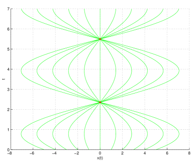
Figure 1: Rays & caustic Harmonic oscillator $V_{h}(x)=x^{2}/2$

The bicharacteristics $(x_{V}(q,p,t),k_{V}(q,p,t))=g^{t}_{V}(q,p)$ for the quartic oscillator are found from the corresponded Hamiltonian system, and they are given by

$$x_{V}(q,p,t)=A(q,p)sd(\Gamma(q,p)t+C(q,p),B(q,p)),\qquad k_{V}(q,p,t)=\frac{\partial x_{V}}{\partial t}(q,p,t)$$ (5.12)

where

$$\begin{array}[]{l}A(q,p)=\frac{\sqrt{c(q,p)}}{(2\mu c(q,p)+1)^{1/4}}\ ,\qquad\qquad B^{2}(q,p)=\frac{\sqrt{2\mu c(q,p)+1}-1}{2\sqrt{2\mu c(q,p)+1}}\ ,\\ \\ \Gamma(q,p)=(2\mu c(q,p)+1)^{1/4}\ ,\qquad\qquad C(q,p)=sd^{-1}(\frac{q}{A(q,p)},B(q,p))\end{array}$$ (5.13)

with

$$c(q,p)=p^{2}+q^{2}+\mu\frac{q^{4}}{2}\ ,$$

and $sd(a,b)=\frac{sn(a,b)}{dn(a,b)}$,$sn,\ dn$ are the Jacobi elliptic functions.

Unfortunately it is not possible to obtain an analytical formula for the caustic. However, by considering the rays $\tilde{x}_{V}=\tilde{x}_{V}(t;q)=x_{V}(q,p=S^{\prime}_{0}(q),t)$ and solving numerically the equation $J(q,t)=\partial_{q}\tilde{x}_{V}=0$, which is available in explicit form, we have observed that the caustic consists of a family of cusps with beaks at the focal points of the corresponding harmonic oscillator (Figure 2). We have checked analytically this observation by proving that the focal points of harmonic oscillator are indeed zeros of the Jacobian for the quartic oscillator.

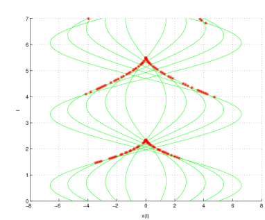
Figure 2: Rays & caustic Quartic oscillator $V(x)=x^{2}/2+\mu x^{4}/4$

Since the expressions of the bicharacteristics for the anharmonic oscillator are very complicated, the analytical computation of coefficient $Z_{c}^{\varepsilon,(l)}(x,k,t)$ of the classical expansion isimpossible. Nevertheless, it is possible to compute the classical expansion of the Wigner function approximately, by using an approximation of the characteristics for small values of the coupling constant $\mu$. Indeed, by the method of multiple scales, for $\mu$ being the small parameter, we solve the ordinary differential equation

$$\ddot{x}+x+\mu x^{3}=0\ ,\ \ x(0)=q\ ,\ \ \dot{x}(0)=p\ ,$$

which, is equivalent to the Hamiltonian system for the quartic oscillator, and we get the following approximation of the bicharacteristics

$$\left\{\begin{array}[]{l}x_{a}(q,p,t)=q\cos(\omega t)+p\sin(\omega t)+O(\mu)\\ k_{a}(q,p,t)=\dot{x}_{a}(q,p,t))=p\omega\cos(\omega t)-q\omega\sin(\omega t)+O(\mu)\ ,\end{array}\right.$$ (5.14)

and also the approximation of the inverse bicharacteristics

$$\left\{\begin{array}[]{l}q_{a}(x,k,t)=x_{a}(x,k,-t)=x\cos(\omega t)-k\sin(\omega t)+O(\mu)\\ p_{a}(x,k,t)=x_{a}(x,k,-t)=k\omega\cos(\omega t)+x\omega\sin(\omega t)+O(\mu)\ ,\end{array}\right.$$ (5.15)

where $\omega=\omega(q,p;\mu)=1+\frac{3}{8}\mu(q^{2}+p^{2})+O(\mu^{2})$ is the approximate angular velocity of the quartic oscillator.

Amplitude via harmonic approximation.

The harmonic expansion of $W^{\varepsilon}(x,k,t)$ reads

$$W^{\varepsilon}(x,k,t)\sim W^{\varepsilon}_{h}(x,k,t)+\sum_{j=1}^{\infty}\varepsilon^{j}Z^{\varepsilon,(2j)}(x,k,t)$$

where

$$W^{\varepsilon}_{h}(x,k,t) = W^{\varepsilon}_{0}(q_{h}(x,k,t),p_{h}(x,k,t))=$$ (5.16)

$$= \frac{1}{\sqrt{\pi}\varepsilon}e^{-(x\cos(t)-k\sin(t))^{2}}e^{-\frac{(k(\cos(t)+\sin(t))-x(\sin(t)-\cos(t)))^{2}}{\varepsilon^{2}}}\ .$$

Integrating $W^{\varepsilon}_{h}$ with respect to $k$ (recall (1.10)), we compute the principal contribution of $W^{\varepsilon}(x,k,t)$ to the amplitude

$$|\psi^{\varepsilon}_{h}(x,t)|^{2}\approx\int_{\mathbb{R}}W^{\varepsilon}_{h}(x,k,t)dk=\frac{1}{\sqrt{\varepsilon^{2}\sin^{2}(t)+(\cos(t)+\sin(t))^{2}}}$$

$$\times exp\left(-x^{2}\frac{(-2\sin^{2}(t)+(\cos(t)+\sin(t))^{2})^{2}}{\varepsilon^{2}\sin^{2}(t)+(\cos(t)+\sin(t))^{2}}\right)\ .$$ (5.17)

At the focal points we have

$$|\psi^{\varepsilon}_{h}(x=0,t_{\nu})|^{2}\approx\frac{\sqrt{2}}{\varepsilon}\ .$$ (5.18)

The coefficient $Z^{\varepsilon,(2)}(x,k,t)$ are computed in Appendix A3, in two different ways which lead to the same approximation up to the order $O(\varepsilon^{2})$. The contribution of this term in the amplitude $|\psi^{\varepsilon}|^{2}$ at the focal points, is also computed in the Appendx A3, and it is given by

$$\varepsilon\int_{\mathbb{R}}Z^{\varepsilon,(2)}(0,k,t_{\nu})dk=\varepsilon\frac{1}{\sqrt{\varepsilon}}\int_{\mathbb{R}}Z^{\varepsilon,(2)}(0,\eta,t_{\nu})d\eta=\frac{\sqrt{2}}{\pi\varepsilon}\mu(\beta+\beta^{\varepsilon})$$ (5.19)

where

$$\beta=\frac{\pi}{8}(\mu-1/4)-3\ ,\qquad\beta^{\varepsilon}=\frac{17}{2}\varepsilon-(\frac{3\pi}{16}(\mu-1/4)+3)\varepsilon^{2}\ .$$

By continuing the computation to higher orders, it turns out that the contribution of the subsequent terms of the expansion is also of the order $O({1}/{\varepsilon})$.

Amplitude via classical approximation.

The classical expansion (4.4) of $W^{\varepsilon}(x,k,t)$ reads

$$\begin{array}[]{l}W^{\varepsilon}(x,k,t)\sim W^{\varepsilon}_{c}(x,k,t)+\sum_{l=1}^{\infty}\varepsilon^{2l}Z_{c}^{\varepsilon,(l)}(x,k,t)\\ \end{array}$$

The leading term $W^{\varepsilon}_{c}(x,k,t)$ and the subsequent coefficients $Z_{c}^{\varepsilon,(l)}(x,k,t)$ are calculated using (4.7) and the approximate characteristics (5.14), and they are given by

$$\begin{array}[]{l}W^{\varepsilon}_{c}(x,k,t)\sim W^{\varepsilon}_{a}(q_{a}(x,k,t),p_{a}(x,k,t)):=W^{\varepsilon}_{0}(q_{a}(x,k,t),p_{a}(x,k,t))\ ,\\ \\ Z_{c}^{\varepsilon,(l)}(x,k,t)=\int_{0}^{t}\Theta^{(l)}(q_{a}(x,k,s-t),p_{a}(x,k,s-t),s)ds\ .\end{array}$$ (5.20)

Integrating $W^{\varepsilon}_{c}$ with respect to $k$, we compute the principal contribution of $W^{\varepsilon}(x,k,t)$ to the amplitude

$$|\psi^{\varepsilon}(0,t_{\nu})|^{2}\approx \int_{\mathbb{R}}W^{\varepsilon}_{a}(0,k,t_{\nu})dk\equiv\int_{\mathbb{R}}W^{\varepsilon}_{0}(q_{a}(0,k,t_{\nu}),p_{a}(0,k,t_{\nu}))dk$$

$$= \frac{1}{\sqrt{\pi}\varepsilon}\int_{\mathbb{R}}e^{-\frac{k^{2}}{2}(1-\mu\gamma k^{2})^{2}}e^{-(\frac{\mu}{\varepsilon})^{2}\alpha^{2}k^{6}}dk$$ (5.21)

$$= \frac{1}{\sqrt{\pi}\varepsilon^{2/3}}\int_{\mathbb{R}}e^{-\frac{\varepsilon^{2/3}\xi^{2}}{2}(1-\mu\gamma\varepsilon^{2/3}\xi^{2})^{2}}e^{-\mu^{2}\alpha^{2}\xi^{6}}d\xi$$

$$= \frac{1}{\sqrt{\pi}\varepsilon^{2/3}\mu^{1/3}}\int_{\mathbb{R}}e^{-\frac{\varepsilon^{2/3}y^{2}}{2\mu^{2/3}}(1-\mu^{1/3}\gamma\varepsilon^{2/3}y^{2})^{2}}e^{-\alpha^{2}y^{6}}dy\ ,$$

where $\gamma,\ \alpha$ are constants independent of $\mu$ and $\varepsilon$.

Hence

$$|\psi^{\varepsilon}(0,t_{\nu})|^{2}\sim O\left(\frac{1}{\varepsilon^{2/3}\mu^{1/3}}\right),\ \textrm{for}\ \mu\sim\varepsilon^{1-\delta},0\leq\delta\leq 1\ ,$$ (5.22)

and

$$|\psi^{\varepsilon}(0,t_{\nu})|^{2}\sim O\left(\frac{1}{\varepsilon}\right),\ \textrm{for}\ \mu\sim\varepsilon^{1+\delta},\ \ \delta\geq 0\ .$$ (5.23)

These estimates have the same order with the corresponding one which was computed from the harmonic expansion if we choose $\mu=O(\varepsilon^{1+\delta})$. Therefore, if we allow the dependence of the coupling constant $\mu$ on the parameter $\varepsilon$, the result shows that for this particular relation between the frequency and the strength of anharmonicity of the potential, both expansions predict the same semiclassical effect, at least at the focal points. However, from the above analysis we also expect agreement of the predicted wave fields everywhere. Moreover, and more important, this picture suggests that different expansions should be used according to the actual relation of the parameters $\varepsilon$ and $\mu$, but it is still open and quite difficult to determine precise criteria for transferring from one approximation to the other.

Finally, it is interesting to remark that the constructed expansions, at least for the example of quartic oscillator, are related as follows

$$W^{\varepsilon}(x,k,t)\xrightarrow{{\varepsilon<<1}}W^{\varepsilon}_{c}(x,k,t)+\sum\varepsilon^{2l}Z_{c}^{\varepsilon,(l)}\ \xrightarrow{{\mu<<1,O(\varepsilon)}}W^{\varepsilon}_{h}(x,k,t)+\sum\varepsilon^{l}Z^{\varepsilon,(2l)}\ .$$ (5.24)

6 Discussion

We have constructed a couple of approximations of the Wigner function for the Schrödinger equation with oscillatory initial data. The first one, which we call the harmonic approximation, has the form

$$W^{\varepsilon}(x,k,t)\sim W^{\varepsilon}_{h}(x,k,t)+\sum_{j=1}^{\infty}\varepsilon^{j}Z^{\varepsilon,(2j)}(x,k,t)$$

where the principal term $W^{\varepsilon}_{h}$ is the Wigner function of a harmonic oscillator associated to the harmonic approximation of the potential $V(x)$. The second one, which has been used in quantum mechanics long time ago. has the multiplicative form

$$W^{\varepsilon}(x,k,t)=W^{\varepsilon}_{c}(x,k,t)\Bigl{(}1+\sum_{\ell\geq 1}\varepsilon^{\ell}W^{\varepsilon}_{\ell}(x,k,t)\Bigr{)}\ ,$$

where $W^{\varepsilon}_{c}$ is the limit Wigner distirbution which is the solution of the Liouville equation of classical mechanics. For the construction of both approximations we choose the initial data for the principal terms to be the initial Wigner function $W^{\varepsilon}(x,k,t=0)=W^{\varepsilon}_{0}(x,k)$, that is $W^{\varepsilon}_{h}(x,k,t=0)=W^{\varepsilon}_{0}(x,k)$ and $W^{\varepsilon}_{c}(x,k,t=0)=W^{\varepsilon}_{0}(x,k)$ . This choice allows us,, after an appropriate scaling of phase space coordinates, to apply a regular perturbation scheme, which, however, has the consequence that the constructed expansions are not genuine semiclassical expansions, because the correctors depend on the small parameter. The expansions are used in the computation of the wave amplitude for a quartic oscillator with WKB data of the Gauss-Fresnel type. They both give reasonable symptomatic approximations at the focal points (caustic) of the oscillator for certain dependence of the coupling constant of the anharmonic potential with the small semiclassical parameter of the Schrödinger equation.

Acknowledgements.

EKK has been partially supported by the Research grant 88735, University of Crete (Programme: Graduate fellowships ”Heraclitus”, funded by the Greek Ministry of Education). GNM has been partially supported by the Archimedes Center for Modeling, Analysis & Computation (ACMAC), Crete, Greece (grant FP7-REGPDT-2009-1). GNM would like to thank R. Littlejohn (Berkeley), R. Schubert (Bristol) and A. Athanassoulis (Leicester) for helpful discussions.

Appendices

Appendix A1:Proof of estimate (2.23)

For the proof of the estimate (2.23) we start from the representation

$$\left[U_{\varepsilon,(xk)}^{-1}\Phi^{\varepsilon}_{nm}\right](\xi,\eta) = \varepsilon\frac{1}{\pi\varepsilon}\int_{\mathbb{R}}e^{-i\frac{2\eta}{\sqrt{\varepsilon}}\sigma}u^{\varepsilon}_{n}(\sqrt{\varepsilon}\xi+\sigma)\overline{u^{\varepsilon}_{m}(\sqrt{\varepsilon}\xi-\sigma)}d\sigma$$

$$= \frac{1}{\pi}\int_{\mathbb{R}}e^{-i2\eta y}\left[U_{\varepsilon}^{-1}u^{\varepsilon}_{n}\right](\xi+y)\left[U_{\varepsilon}^{-1}u^{\varepsilon}_{m}\right](\xi-y)dy\ ,$$ (A1.1)

and we use the identity

$$\begin{array}[]{l}\left[U_{\varepsilon}^{-1}u^{\varepsilon}_{n}\right](\eta)\left[U_{\varepsilon}^{-1}u^{\varepsilon}_{m}\right](\xi)-\sum\limits_{l=0}^{N}\varepsilon^{\frac{l}{2}}\sum\limits_{\mu=0}^{l}\psi_{n}^{(\mu)}(\eta)\psi_{m}^{(l-\mu)}(\xi)\\ =\left(\left[U_{\varepsilon}^{-1}u^{\varepsilon}_{n}\right](\eta)-\sum\limits_{l=0}^{N}\varepsilon^{\frac{l}{2}}\psi_{n}^{(l)}(\eta)\right)\left(\left[U_{\varepsilon}^{-1}u^{\varepsilon}_{m}\right](\xi)-\sum\limits_{l=0}^{N}\varepsilon^{\frac{l}{2}}\psi_{m}^{(l)}(\xi)\right)\\ +\left(\left[U_{\varepsilon}^{-1}u^{\varepsilon}_{n}\right](\eta)-\sum\limits_{l=0}^{N}\varepsilon^{\frac{l}{2}}\psi_{n}^{(l)}(\eta)\right)\sum\limits_{l=0}^{N}\varepsilon^{\frac{l}{2}}\psi_{m}^{(l)}(\xi)\\ +\left(\left[U_{\varepsilon}^{-1}u^{\varepsilon}_{m}\right](\xi)-\sum\limits_{l=0}^{N}\varepsilon^{\frac{l}{2}}\psi_{m}^{(l)}(\xi)\right)\sum\limits_{l=0}^{N}\varepsilon^{\frac{l}{2}}\psi_{n}^{(l)}(\eta)\\ +\sum\limits_{l=N+1}^{2N}\varepsilon^{\frac{l}{2}}\sum\limits_{\mu=l-N}^{N}\psi_{n}^{(\mu)}(\eta)\psi_{m}^{(l-\mu)}(\xi)\ .\end{array}$$ (A1.2)

Then, we have

$$\begin{array}[]{l}||\left[U_{\varepsilon,(xk)}^{-1}\Phi^{\varepsilon}_{nm}\right]-\sum\limits_{l=0}^{N}\varepsilon^{\frac{l}{2}}{\widetilde{Z}}_{nm}^{(l)}||^{2}_{L^{2}(\mathbb{R}^{2})}\\ =\int_{\mathbb{R}}\int_{\mathbb{R}}|\left[U_{\varepsilon,(xk)}^{-1}\Phi^{\varepsilon}_{nm}\right](\xi,\eta)-\sum\limits_{l=0}^{N}\varepsilon^{\frac{l}{2}}{\widetilde{Z}}_{nm}^{(l)}(\xi,\eta)|^{2}d\xi d\eta\\ =\int_{\mathbb{R}}\int_{\mathbb{R}}|\frac{1}{\pi}\int_{\mathbb{R}}e^{-i2\eta y}\left(\left[U_{\varepsilon}^{-1}u^{\varepsilon}_{n}\right](\xi+y)\left[U_{\varepsilon}^{-1}u^{\varepsilon}_{m}\right](\xi-y)-\sum\limits_{l=0}^{N}\varepsilon^{\frac{l}{2}}\sum\limits_{\mu=0}^{l}\psi_{n}^{(\mu)}(\xi+y)\psi_{m}^{(l-\mu)}(\xi-y)\right)dy|^{2}d\xi d\eta\\ =\int_{\mathbb{R}}\int_{\mathbb{R}}|\left[U_{\varepsilon}^{-1}u^{\varepsilon}_{n}\right](\xi+y)\left[U_{\varepsilon}^{-1}u^{\varepsilon}_{m}\right](\xi-y)-\sum\limits_{l=0}^{N}\varepsilon^{\frac{l}{2}}\sum\limits_{\mu=0}^{l}\psi_{n}^{(\mu)}(\xi+y)\psi_{m}^{(l-\mu)}(\xi-y)|^{2}d\xi dy\\ =\int_{\mathbb{R}}\int_{\mathbb{R}}|\left[U_{\varepsilon}^{-1}u^{\varepsilon}_{n}\right](\eta)\left[U_{\varepsilon}^{-1}u^{\varepsilon}_{m}\right](\xi)-\sum\limits_{l=0}^{N}\varepsilon^{\frac{l}{2}}\sum\limits_{\mu=0}^{l}\psi_{n}^{(\mu)}(\eta)\psi_{m}^{(l-\mu)}(\xi)|^{2}d\eta d\xi\\ \leq||[U_{\varepsilon}^{-1}u^{\varepsilon}_{n}]-\sum\limits_{l=0}^{N}\varepsilon^{\frac{l}{2}}\psi_{n}^{(l)}||^{2}_{L^{2}(\mathbb{R})}||[U_{\varepsilon}^{-1}u^{\varepsilon}_{m}]-\sum\limits_{l=0}^{N}\varepsilon^{\frac{l}{2}}\psi_{m}^{(l)}||^{2}_{L^{2}(\mathbb{R})}\\ +||[U_{\varepsilon}^{-1}u^{\varepsilon}_{n}]-\sum\limits_{l=0}^{N}\varepsilon^{\frac{l}{2}}\psi_{n}^{(l)}||^{2}_{L^{2}(\mathbb{R})}\sum\limits_{l=0}^{N}\varepsilon^{\frac{l}{2}}||\psi_{m}^{(l)}||^{2}_{L^{2}(\mathbb{R})}+||[U_{\varepsilon}^{-1}u^{\varepsilon}_{m}]-\sum\limits_{l=0}^{N}\varepsilon^{\frac{l}{2}}\psi_{m}^{(l)}||^{2}_{L^{2}(\mathbb{R})}\sum\limits_{l=0}^{N}\varepsilon^{\frac{l}{2}}||\psi_{n}^{(l)}||^{2}_{L^{2}(\mathbb{R})}\\ +\sum\limits_{l=N+1}^{2N}\varepsilon^{\frac{l}{2}}\sum\limits_{\mu=l-N}^{N}||\psi_{n}^{(\mu)}||^{2}_{L^{2}(\mathbb{R})}||\psi_{m}^{(l-\mu)}||^{2}_{L^{2}(\mathbb{R})}\ .\end{array}$$ (A1.3)

Now since $\psi_{n}^{(\mu)}\in L^{2}(\mathbb{R}),\ \mu=0,1,\dots,\ \ n=0,1,\dots$ and

$$||[U_{\varepsilon}^{-1}u^{\varepsilon}_{m}]-\sum\limits_{l=0}^{N}\varepsilon^{\frac{l}{2}}\psi_{m}^{(l)}||^{2}_{L^{2}(\mathbb{R})}=O(\varepsilon^{(N+1)/2})\ ,$$ (A1.4)

we obtain the desired estimate.

Appendix A2: Proof of Theorems 2 & 3

In the sequel we denote by $\|\cdot\|$ the norms $\|\cdot\|_{L^{2}_{r^{\varepsilon}}}$ or $\|\cdot\|_{L^{2}}$ and we write them explicitly when the distinction is necessary. The constants $C_{N}$ are of the generic form $cN!N^{\alpha}$, with $\alpha>0\ ,\ \ c>0$ (see also [10]).

For the proof of the Theorems 2 and 3 we need the following lemmas and propositions.

Lemma 1.

(Faa di Bruno formula, [12] , [10], [29]).

Let $f:\mathbb{R}^{2}\rightarrow\mathbb{R},\ g:\mathbb{R}^{2}\rightarrow\mathbb{R}^{2}$ smooth enough functions. For any multi-index $\nu\in\mathbb{N}^{2}$ and $z=(\xi,\eta)\in\mathbb{R}^{2}$ ,

$$\partial^{\nu}\left(f\circ g\right)(z)=\sum_{0\neq|\gamma|\leq|\nu|,\ \gamma\in\mathbb{N}^{2}}\left[(\partial^{\gamma}f)\circ g\right](z)B_{\nu,\gamma}\left[\partial g\right](z)$$ (A2.1)

where

$$B_{\nu,\gamma}\left[\partial g\right]=\nu!\sum_{\alpha_{\beta}}\prod_{\beta\neq 0}\frac{1}{\alpha_{\beta}!}\left(\frac{\partial^{\beta}g_{1}}{\beta!}\right)^{\alpha_{\beta_{1}}}\left(\frac{\partial^{\beta}g_{2}}{\beta!}\right)^{\alpha_{\beta_{2}}}$$ (A2.2)

with $\beta=(\beta_{1},\beta_{2}),\ \alpha_{\beta}=(\alpha_{\beta_{1}},\alpha_{\beta_{2}})$

$$\quad\sum\alpha_{\beta_{1}}=\gamma_{1},\ \sum\alpha_{\beta_{2}}=\gamma_{2},\ \sum\beta_{1}\alpha_{\beta_{1}}=\nu_{1},\ \sum\beta_{2}\alpha_{\beta_{2}}=\nu_{2}.$$

Lemma 2.

For the Hamiltonian flow $g_{h}^{t}=g_{h}^{t}(\xi,\eta)$ of the harmonic oscillator, and for all $(\xi,\eta)$ and $t>0$, hold

1. $$\begin{array}[]{l}|\partial_{\eta}g_{h,i}^{\pm t}|\leq 1,\quad|\partial_{\xi}g_{h,i}^{\pm t}|\leq 1\ ,\\ \\ \partial^{\nu}_{\eta}g_{h,i}^{\pm t}=\mathbb{O}_{\nu\times\nu},\quad\partial^{\nu}_{\xi}g_{h,i}^{\pm t}=\mathbb{O}_{\nu\times\nu},\ \ i=1,2,\ \nu=2,3,\dots\ .\end{array}$$ (A2.3)

   where $\mathbb{O}_{\nu\times\nu}$ denotes the ${\nu\times\nu}$ zero matrix.

2. $$|g_{h,i}^{\pm t}(\xi,\eta)|^{\nu}\leq(|\xi|+|\eta|)^{\nu},\ i=1,2,\ \nu=1,2,\dots$$ (A2.4)

3. $$\left|B_{\nu,\gamma}\left[\partial g_{h}^{-t}\right]\right|\leq C_{\nu,\gamma}$$ (A2.5)

   where $B_{\nu,\gamma}$ are defined in the the previouss Lemma 1, and

4. For all $f\in\mathcal{S}(\mathbb{R}^{2})$

   $$\|f(g_{h}^{-t})\|=\|f\|$$ (A2.6)

The proof of Lemma 2 is based on a straightforward computation.

Lemma 3.

1. For all $\widetilde{f}_{0}(\xi,\eta)\in\mathcal{S}(\mathbb{R}^{2})$ and $m\geq 1$ holds

   $$\|(|\xi|+|\eta|)^{m}\partial^{\beta}\widetilde{f}_{0}\|_{L^{2}}\leq C_{m,\beta}$$

2. For $\widetilde{f}^{\varepsilon}_{0}(\xi,\eta)$ as in Theorem 3 holds

   $$\|(|\xi|+|\eta|)^{m}\partial^{\beta}\widetilde{f}^{\varepsilon}_{0}\|_{L^{2}_{r^{\varepsilon}}}\leq\varepsilon^{m+1}C_{\beta}$$

where $\beta=(\beta_{1},\beta_{2})\in\mathbb{N}^{2},\ \ \partial^{\beta}f=\partial^{\beta_{1}}_{\xi}\partial^{\beta_{2}}_{\eta}f$

Proof of Lemma 3:

The first part of Lemma 3 is immediate, since $\widetilde{f}_{0}(\xi,\eta)\in\mathcal{S}(\mathbb{R}^{2})$. The proof of the second part, relies on direct computation using the explicit form of $\widetilde{f}^{\varepsilon}_{0}(\xi,\eta)$. We show the details for the case $\alpha_{0}(x)=e^{-x^{2}/2}$ and $S_{0}(x)=x^{2}/2$. For the case of $S_{0}(x)=x$ we proceed similarly. For

$$\widetilde{f}^{\varepsilon}_{0}(\xi,\eta)=\frac{1}{\pi}e^{-\varepsilon\xi^{2}}e^{-\frac{(\eta-\xi)^{2}}{\varepsilon}}$$

and for any $\beta=(\beta_{1},\beta_{2})\in\mathbb{N}^{2}$, $\beta\neq 0$, we have

$$\begin{array}[]{l}\partial^{\beta}\widetilde{f}^{\varepsilon}_{0}(\xi,\eta)=(\sqrt{\varepsilon})^{-|\beta|}\frac{(-2i)^{\beta_{2}}2^{-|\beta|}e^{i|\beta|\pi/2}}{\sqrt{\pi}}e^{-\varepsilon\xi^{2}}e^{-\frac{(\eta-\xi)^{2}}{\varepsilon}}\\ \times\sum_{j=0}^{\beta_{1}}\left({\begin{matrix}\beta_{1}\\ j\\ \end{matrix}}\right)(-2)^{j}e^{-ij\pi/2}H_{j}(\sqrt{\varepsilon}\xi)H_{|\beta|-j}\left(\frac{\eta-\xi}{\sqrt{\varepsilon}}\right)\end{array}$$

where $H_{j}$ are the Hermite polynomials.

The term that dominates $\partial^{\beta}\widetilde{f}^{\varepsilon}_{0}(\xi,\eta)$ for small values of $\varepsilon$, is

$$G_{\beta}^{\varepsilon}(\xi,\eta)=\varepsilon^{-|\beta|}c_{\beta}e^{-\varepsilon\xi^{2}}e^{-\frac{(\eta-\xi)^{2}}{\varepsilon}}(\eta-\xi)^{|\beta|}\ ,$$

with $c_{\beta}=(-2i)^{\beta_{2}}2^{-|\beta|}e^{i|\beta|\pi/2}/\sqrt{\pi}$.

Therefore it is enough to prove a bound for the term $(|\xi|+|\eta|)^{m}G_{\beta}^{\varepsilon}$. We have

$$\|(|\xi|+|\eta|)^{m}\partial^{\beta}\widetilde{f}^{\varepsilon}_{0}\|_{L^{2}_{r^{\varepsilon}}}\leq\sum_{j=1}^{m}\||\xi|^{j}|\eta|^{m-j}\partial^{\beta}\widetilde{f}^{\varepsilon}_{0}\|_{L^{2}_{r^{\varepsilon}}}\sim\sum_{j=1}^{m}\||\xi|^{j}|\eta|^{m-j}G_{\beta}^{\varepsilon}\|_{L^{2}_{r^{\varepsilon}}}\ ,$$

and

$$\begin{array}[]{l}\||\xi|^{j}|\eta|^{m-j}G_{\beta}^{\varepsilon}\|^{2}_{L^{2}_{r^{\varepsilon}}}\\ =c_{\beta}^{2}\varepsilon^{-2|\beta|}\int_{\mathbb{R}}\int_{\mathbb{R}}|\xi|^{2j}|\eta|^{2(m-j)}(\eta-\xi)^{2|\beta|}e^{-2\varepsilon\xi^{2}}e^{-\frac{2(\eta-\xi)^{2}}{\varepsilon}}e^{-\frac{\xi^{2}+\eta^{2}}{\varepsilon^{2}}}d\xi d\eta\\ =c_{\beta}^{2}\varepsilon^{-2|\beta|+2|\beta|+2m+2}\int_{\mathbb{R}}\int_{\mathbb{R}}|\xi|^{2j}|\eta|^{2(m-j)}(\eta-\xi)^{2|\beta|}e^{-2\varepsilon^{3}\xi^{2}}e^{-2\varepsilon(\eta-\xi)^{2}}e^{-(\xi^{2}+\eta^{2})}d\xi d\eta\\ =\varepsilon^{2m+2}c_{\beta}^{2}c^{\varepsilon}\ ,\\ \end{array}$$

where $c^{\varepsilon}\to c<\infty$, as $\varepsilon\to 0$. This concludes the proof of

$$\|(|\xi|+|\eta|)^{m}\partial^{\beta}\widetilde{f}^{\varepsilon}_{0}\|_{L^{2}_{r^{\varepsilon}}}\leq\varepsilon^{m+1}C_{\beta}$$

$\blacksquare$

Proposition 1.

1. For all $f\in\mathcal{S}(\mathbb{R}^{2})$ and $\nu_{j}\in\mathbb{N},\ \ j=1,2\dots$ holds

   $$\|\mathcal{B}_{\nu_{1}}\left[\mathcal{B}_{\nu_{2}}\left[\dots\mathcal{B}_{\nu_{j}}\left[f(g_{h}^{-t_{j+1}})\right]\dots\right](g_{h}^{-(t_{1}-t_{2})},t_{2})\right](g_{h}^{-(t-t_{1})},t_{1})\|_{L^{2}}\leq C_{\nu_{1},\dots,\nu_{j}}$$ (A2.7)

2. For $\widetilde{f}^{\varepsilon}_{0}(\xi,\eta)$ as in Theorem · 3, and $\nu_{j}\in\mathbb{N},\ \ j=1,2\dots$ holds

   $$\|\mathcal{B}_{\nu_{1}}\left[\mathcal{B}_{\nu_{2}}\left[\dots\mathcal{B}_{\nu_{j}}\left[f(g_{h}^{-t_{j+1}})\right]\dots\right](g_{h}^{-(t_{1}-t_{2})},t_{2})\right](g_{h}^{-(t-t_{1})},t_{1})\|_{L^{2}_{r^{\varepsilon}}}\leq C_{\nu_{1},\dots,\nu_{j}}$$ (A2.8)

Proof of Proposition 1:

Recall that the operators $\mathcal{B}_{\nu_{j}}$ are given by the formula

$$\mathcal{B}_{\nu_{j}}=-V^{(\nu_{j}+2)}(0)\sum\limits_{\lambda_{j}=0}^{[(\nu_{j}-1)/2]+1}c_{\lambda_{j},\nu_{j}}\xi^{\nu_{j}+1-2\lambda_{j}}\frac{\partial^{(2\lambda_{j}+1)}}{\partial{\eta^{2\lambda_{j}+1}}}\ ,$$

with $c_{\lambda_{j},\nu_{j}}=\left(\frac{i}{2}\right)^{2\lambda_{j}}\frac{1}{(2\lambda_{j}+1)!(\nu_{j}+1-2\lambda_{j})!}\ .$

By Lemma 2, the left hand side of (A2.7), (A2.8) reads as

$$\|\mathcal{B}_{\nu_{1}}\left[\mathcal{B}_{\nu_{2}}\left[\dots\mathcal{B}_{\nu_{j}}\left[f(g_{h}^{-t_{j+1}})\right]\dots\right](g_{h}^{-(t_{1}-t_{2})},t_{2})\right]\parallel\ ,$$

and hence it is enough to estimate this quantity. First we prove (A2.7) for all $j$. We give the details only for the cases $j=1$ and $j=2$. For $j=1$ we have,

$$\|\mathcal{B}_{\nu_{1}}\left[f(g_{h}^{-t_{1}})\right]\|_{L^{2}} \leq|V^{(\nu_{1}+2)}(0)|\sum\limits_{\lambda_{j}=0}^{[(\nu_{1}-1)/2]+1}c_{\lambda_{1},\nu_{1}}\|\xi^{\nu_{1}+1-2\lambda_{1}}\frac{\partial^{(2\lambda_{1}+1)}}{\partial{\eta^{2\lambda_{1}+1}}}f(g_{h}^{-t_{1}})\|_{L^{2}}$$

$$\leq\sum\limits_{\lambda_{j}=0}^{[(\nu_{1}-1)/2]+1}c_{\lambda_{1},\nu_{1}}\sum_{0\neq|\gamma|\leq\nu_{1}}C^{\prime}_{\nu_{1},\gamma}\|\xi^{\nu_{1}+1-2\lambda_{1}}\left[(\partial^{\gamma}f)\circ g_{h}^{-t}\right](z)\left|B_{\nu_{1},\gamma}\left[\partial g_{h}^{-t}\right]\right|\|_{L^{2}}$$

$$\leq\sum\limits_{\lambda_{j}=0}^{[(\nu_{1}-1)/2]+1}c_{\lambda_{1},\nu_{1}}\sum_{0\neq|\gamma|\leq\nu_{1}}C_{\nu_{1},\gamma}\|(g_{h,1}^{-t})^{\nu_{1}+1-2\lambda_{1}}\partial^{\gamma}f(z)\|_{L^{2}}$$

$$=\sum\limits_{\lambda_{j}=0}^{[(\nu_{1}-1)/2]+1}c_{\lambda_{1},\nu_{1}}\sum_{0\neq|\gamma|\leq\nu}C_{\nu_{1},\gamma}\|(|\xi|+|\eta|)^{\nu_{1}+1-2\lambda_{1}}\partial^{\gamma}f(z)\|_{L^{2}}$$

where in the first step we used Faa di Bruno formula, and the then (A2.4),(A2.5).

The first part of Lemma 3 ensures that

$$\|(|\xi|+|\eta|)^{\nu_{1}+1-2\lambda_{1}}(\partial^{\gamma}f(z)\|_{L^{2}}\leq C_{\lambda_{1},\nu_{1},\gamma}\ ,$$

thus

$$\|\mathcal{B}_{\nu_{1}}\left[f(g_{h}^{-t_{1}})\right]\|_{L^{2}}\leq|V^{(\nu_{1}+2)}(0)|\sum\limits_{\lambda_{1}=0}^{[(\nu_{1}-1)/2]+1}c_{\lambda_{1},\nu_{1}}C_{\lambda_{1},\nu_{1}}\leq C_{\nu_{1}}\ ,$$

which proves (A2.7) for $j=1$.

For $j=2$, we have

$$\| \mathcal{B}_{\nu_{1}}\left[\mathcal{B}_{\nu_{2}}\left[f(g_{h}^{-t_{2}})\right](g_{h}^{-(t_{1}-t_{2})})\right]\|\leq$$

$$\leq|V^{(\nu_{1}+2)}(0)|\sum\limits_{\lambda_{j}=0}^{[(\nu_{1}-1)/2]+1}c_{\lambda_{1},\nu_{1}}\sum_{|\beta^{1}|\leq 2\lambda_{1}+1}c_{\beta}\|(|\xi|+|\eta|)^{\nu_{1}+1-2\lambda_{1}}\partial^{\beta}\left[\mathcal{B}_{\nu_{2}}\left[f(g_{h}^{-t_{2}})\right]\right]\|$$

$$\leq|V^{(\nu_{1}+2)}(0)||V^{(\nu_{2}+2)}(0)|\sum\limits_{\lambda_{1}=0}^{[(\nu_{1}-1)/2]+1}\sum\limits_{\lambda_{2}=0}^{[(\nu_{2}-1)/2]+1}c_{\lambda_{1},\nu_{1}}c_{\lambda_{2},\nu_{2}}$$

$$\sum_{|\beta^{1}|\leq 2\lambda_{1}+1}c_{\beta}\|(|\xi|+|\eta|)^{\nu_{1}+1-2\lambda_{1}}\partial^{\beta}\left[\xi^{\nu_{2}+1-2\lambda_{2}}\partial_{\eta}^{2\lambda_{2}+1}\left[f(g_{h}^{-t_{2}})\right]\right]\|$$

$$\leq\prod_{i=1,2}|V^{(\nu_{i}+2)}(0)|\sum\limits_{\lambda_{1}=0}^{\nu_{1}^{\ell}}\sum\limits_{\lambda_{2}=0}^{\nu_{2}^{\ell}}\sum_{|\beta^{1}|\leq u^{1}}\sum_{\alpha_{1}=0}^{\beta_{1}}\sum_{|\beta^{2}|\leq u^{2}}C(\nu_{1},\nu_{2},\lambda_{1},\beta^{1},\beta^{2},\alpha_{1})\|(|\xi|+|\eta|)^{\gamma_{1}}\partial^{\beta^{2}}f\|$$

where

$$\nu_{i}^{\ell}=[(\nu_{i}-1)/2]+1,\ \beta^{i}\in\mathbb{N}^{2},\ u^{1}=\lambda_{1}+1,\ u^{2}=(\beta^{1}_{1}-\alpha_{1},\beta^{1}_{2}+\lambda_{2}+1)\ ,$$

and

$$\gamma_{1}=\nu_{1}+\nu_{2}+2-2\lambda_{1}-2\lambda_{2}-\alpha_{1}\ .$$

Therefore

$$\|\mathcal{B}_{\nu_{1}}\left[\mathcal{B}_{\nu_{2}}\left[f(g_{h}^{-t_{2}})\right](g_{h}^{-(t_{1}-t_{2})})\right]\|_{L^{2}}\leq C_{\nu_{1},\nu_{2}}\ .$$

In the same way we can prove it for the general case for all $j\geq 3$, by applying successively the Faa di Bruno formula, the Leibniz formula and using Lemma 2, to get

$$\|\mathcal{B}_{\nu_{1}}\left[\mathcal{B}_{\nu_{2}}\left[\dots\mathcal{B}_{\nu_{j}}\left[f(g_{h}^{-t_{j+1}})\right]\dots\right](g_{h}^{-(t_{1}-t_{2})},t_{2})\right](g_{h}^{-(t-t_{1})},t_{1})\|_{L^{2}}\leq$$ (A2.9)

$$\leq\prod_{i=1}^{j}|V^{(\nu_{i}+2)}(0)|\sum\limits_{\lambda_{1}=0}^{\nu_{1}^{\ell}}\sum_{|\beta^{1}|\leq u^{1}}\dots\sum\limits_{\lambda_{j}=0}^{\nu_{j}^{\ell}}\sum_{\alpha_{j-1}}\sum_{|\beta^{j}|\leq u^{j}}C(\nu_{i},\lambda_{i},\beta^{i},\alpha_{i})\|(|\xi|+|\eta|)^{\gamma_{j-1}}\partial^{\beta^{j}}f\|_{L^{2}}\leq C_{\nu_{1},\dots,\nu_{j}}$$

with

$$\nu_{i}^{\ell}=[(\nu_{i}-1)/2]+1,\ \beta^{i}\in\mathbb{N}^{2}\ ,$$

and

$$\gamma_{i}=\sum_{k=1}^{i}(\nu_{k}+1-2\lambda_{k})-\sum_{k=1}^{i-1}\alpha_{k}\ .$$

For proving the second part we follow the same procedure as before, by using the second part of Lemma 3. To proceed we observe that $\|(|\xi|+|\eta|)^{\gamma_{j-1}}\partial^{\beta^{j}}f\|_{L^{2}_{r^{\varepsilon}}}\leq\varepsilon^{\gamma_{j-1}+1}C_{\beta^{j}}$. This estimate and the fact that ${\gamma_{j-1}}$ in (A2.9) is always non-negative, ensure that

$$\|\mathcal{B}_{\nu_{1}}\left[\mathcal{B}_{\nu_{2}}\left[\dots\mathcal{B}_{\nu_{j}}\left[f(g_{h}^{-t_{j+1}})\right]\dots\right](g_{h}^{-(t_{1}-t_{2})},t_{2})\right](g_{h}^{-(t-t_{1})},t_{1})\|_{L^{2}_{r^{\varepsilon}}}\leq C_{\nu_{1},\dots,\nu_{j}}\ ,$$

which ends the proof of the proposition. $\blacksquare$

Proof of Theorem 2:

The $(N+1)$-order remainder (3.19) of the asymptotic expansion (3.18), that is

$$R^{N+1}(\xi,\eta,t):={\widetilde{W}}^{\varepsilon}(\xi,\eta,t)-\sum_{l=0}^{N}\varepsilon^{l/2}{\widetilde{Z}}^{\varepsilon,(l)}(\xi,\eta,t),\ \ N=0,1,\dots\ ,$$

solves, for aany $N$, the initial value problem

$$\frac{\partial}{\partial t}{R^{N+1}}(\xi,\eta,t)+L_{h}R^{N+1}(\xi,\eta,t)=-\sum_{\nu=1}^{N+1}\mathcal{B}_{\nu}\left[R^{N+1-\nu}\right](\xi,\eta,t)$$ (A2.10)

$$R^{N+1}(\xi,\eta,t)|_{t=0}=0$$ (A2.11)

where $R^{0}={\widetilde{W}}^{\varepsilon}_{h}\ \ \text{and}\ \ \mathcal{B}_{\nu}:=\mathcal{B}_{\nu}(\xi,\frac{\partial}{\partial{\eta}})$.

According to Dunhamel’s principle the solution of problem (A2.10), is given by the formula

$$R^{N+1}(\xi,\eta,t)=-\int_{0}^{t}\sum_{\nu=1}^{N+1}\varepsilon^{\nu/2}\mathcal{B}_{\nu}\left[R^{N+1-\nu}\right](g_{h}^{-(t-s)}(\xi,\eta),s)ds,\ \ N=0,1,\dots$$

Applying the above formula successively for each $R^{N+1-\nu}$, we have

$$R^{N+1}(\xi,\eta,t)=\varepsilon^{\frac{N+1}{2}}\left\{-\int_{0}^{t}dt_{1}\mathcal{B}_{N+1}\left[\widetilde{f}_{0}(g_{h}^{-t_{1}})\right]\left(g_{h}^{-(t-t_{1})},t_{1}\right)\right.$$

$$+\int_{0}^{t}dt_{1}\int_{0}^{t_{1}}dt_{2}\mathcal{B}_{N}\left[\mathcal{B}_{1}\left[\widetilde{f}_{0}(g_{h}^{-t_{2}})\right]\left(g_{h}^{-(t_{1}-t_{2})},t_{2}\right)\right]\left(g_{h}^{-(t-t_{1})},t_{1}\right)$$

$$+\int_{0}^{t}dt_{1}\int_{0}^{t_{1}}dt_{2}\mathcal{B}_{N-1}\left[\mathcal{B}_{2}\left[\widetilde{f}_{0}(g_{h}^{-t_{2}})\right]\left(g_{h}^{-(t_{1}-t_{2})},t_{2}\right)\right]\left(g_{h}^{-(t-t_{1})},t_{1}\right)dt_{1}dt_{2}$$

$$-\int_{0}^{t}dt_{1}\int_{0}^{t_{1}}dt_{2}\int_{0}^{t_{2}}dt_{3}\mathcal{B}_{N-1}\left[\mathcal{B}_{1}\left[\mathcal{B}_{1}\left[\widetilde{f}_{0}(g_{h}^{-t_{3}})\right]\left(g_{h}^{-(t_{2}-t_{3})},t_{3}\right)\right]\left(g_{h}^{-(t_{1}-t_{2})},t_{2}\right)\right]\left(g_{h}^{-(t-t_{1})},t_{1}\right)$$

$$+\dots$$

$$\left.+(-1)^{N}\int_{0}^{t}dt_{1}\int_{0}^{t_{1}}dt_{2}\dots\int_{0}^{t_{N}}dt_{N+1}\mathcal{B}_{1}\left[\mathcal{B}_{1}\left[\dots\mathcal{B}_{1}\left[\widetilde{f}_{0}(g_{h}^{-t_{N+1}})\right]\dots\right]\left(g_{h}^{-(t_{1}-t_{2})},t_{2}\right)\right]\left(g_{h}^{-(t-t_{1})},t_{1}\right)\right\}$$

where $\widetilde{f}_{0}(\xi,\eta)$ are the initial data of the problem (3.14).

Hence

$$\|R^{N+1}(\xi,\eta,t)\|_{L^{2}}\leq\varepsilon^{\frac{N+1}{2}}\left\{\int_{0}^{t}dt_{1}\|\mathcal{B}_{N+1}\left[f_{0}(g_{h}^{-t_{1}})\right](g_{h}^{-(t-t_{1})},t_{1})\|_{L^{2}}\right.$$

$$+\int_{0}^{t}dt_{1}\int_{0}^{t_{1}}dt_{2}\|\mathcal{B}_{N}\left[\mathcal{B}_{1}\left[f_{0}(g_{h}^{-t_{2}})\right](g_{h}^{-(t_{1}-t_{2})},t_{2})\right](g_{h}^{-(t-t_{1})},t_{1})\|_{L^{2}}$$

$$+\dots$$

$$+\left.\int_{0}^{t}dt_{1}\int_{0}^{t_{1}}dt_{2}\dots\int_{0}^{t_{N}}dt_{N+1}\|\mathcal{B}_{1}\left[\mathcal{B}_{1}\left[\dots\mathcal{B}_{1}\left[f_{0}(g_{h}^{-t_{N+1}})\right]\dots\right](g_{h}^{-(t_{1}-t_{2})},t_{2})\right](g_{h}^{-(t-t_{1})},t_{1})\|_{L^{2}}\right\}$$

Since $\widetilde{f}_{0}(\xi,\eta)\in\mathcal{S}(\mathbb{R}^{2})$ and $\varepsilon$-independent, the first part of Proposition 1 implies that every term in the right hand side of the above inequality is bounded, and therefore we get

$$\|R^{N+1}(\xi,\eta,t)\|_{L^{2}} \leq\varepsilon^{\frac{N+1}{2}}C_{N}\left\{\int_{0}^{t}dt_{1}+\int_{0}^{t}dt_{1}\int_{0}^{t_{1}}dt_{2}+\dots+\int_{0}^{t}dt_{1}\dots\int_{0}^{t_{N}}dt_{N+1}\right\}\ ,$$

$$=\varepsilon^{\frac{N+1}{2}}C_{N}\sum_{k=1}^{N+1}\frac{t^{k}}{k!}=\varepsilon^{\frac{N+1}{2}}C_{N}e^{t}\ ,$$

which ends the proof. $\blacksquare$

Proof of Theorem 3:

For $\alpha_{0}(x)=e^{-x^{2}/2}$ and $S_{0}(x)=x^{2}/2$, we have

$$\widetilde{f^{\varepsilon}}_{0}(\xi,\eta)=\frac{1}{\sqrt{\pi}}e^{-\varepsilon\xi^{2}}e^{-\frac{(\eta-\xi)^{2}}{\varepsilon}}\ ,$$

while for $S_{0}(x)=x$ we have

$$\widetilde{f^{\varepsilon}}_{0}(\xi,\eta)=\frac{1}{\sqrt{\pi}}e^{-\varepsilon\xi^{2}}e^{-\frac{(\eta-1)^{2}}{\varepsilon}}\ .$$

In both cases $\widetilde{f^{\varepsilon}}_{0}(\xi,\eta)\in\mathcal{S}(\mathbb{R}^{2})$. So we proceed similarly to the proof of Theorem 2 and we use the second part of Proposition 1, to obtain

$$\|R^{N+1}(\xi,\eta,t)\|_{L^{2}_{r^{\varepsilon}}} \leq\varepsilon^{\frac{N+1}{2}}C_{N}\left\{\int_{0}^{t}dt_{1}+\int_{0}^{t}dt_{1}\int_{0}^{t_{1}}dt_{2}+\dots+\int_{0}^{t_{N}}dt_{N+1}\right\}\Rightarrow$$

$$=\varepsilon^{\frac{N+1}{2}}C_{N}e^{t}\ ,$$

which ends the proof of Theorem 3. $\blacksquare$

Appendix A3: Expansion of $Z^{\varepsilon,(2)}$

In this appendix we compute the coefficient $Z^{\varepsilon,(2)}$ of the harmonic expansion in the case of the quartic oscillator . This computation is performed by solving the problem (3.15) with $\ell=2$, that is

$$\Bigl{(}\frac{\partial}{\partial t}+L_{h}\Bigr{)}{\widetilde{Z}}^{\varepsilon,(2)}(\xi,\eta,t)=D^{(2)}(\xi,\eta,t)$$

$${\widetilde{Z}}^{\varepsilon,(2)}(\xi,\eta,t)|_{t=0}=0\ ,$$ (A4.1)

in two different ways.

First way:

We expand ${\widetilde{Z}}^{\varepsilon,(2)}$ with respect to the Moyal eigenfunctions $\Psi_{n}m$ of the harmonic oscillator,

$${\widetilde{Z}}^{\varepsilon,(2)}(\xi,\eta,t)=\sum_{n}\sum_{m}z_{nm}^{\varepsilon}(t)\Psi_{nm}(\xi,\eta)\ ,$$ (A4.2)

and we substitute this series into (Appendix A3: Expansion of $Z^{\varepsilon,(2)}$), together with the eigenfunction series (3.13) of ${\widetilde{W}}^{\varepsilon}_{h}$, which appears in the $D^{(2)}(\xi,\eta,t)$. Then we use the orthogonality of $\Psi_{nm}$ to derive a hierarchy of equations for the coefficients $z_{nm}^{\varepsilon}(t)\ ,\ \ n,m=0,1,\dots\ .$

These equations can be easily integrated because of the polynomial type of the potential and the special form of Moyal eigenfunctions (Laguerre polynomials), and, after a long and cumbersome computation, we get

$${\widetilde{Z}}^{\varepsilon,(2)}(\xi,\eta,t) =-\frac{\mu}{4\pi}Re\left(\sum_{n}\sum_{m}z_{nm}^{\varepsilon}(t)e^{-i(n-m)t}\Psi^{\varepsilon}_{nm}(\xi,\eta)\right)+$$

$$+\frac{3\mu}{4\pi}tIm\left(\sum_{n}\sum_{m}A_{h,nm,o}^{\varepsilon}(n^{2}+n)e^{-i(n-m)t}\Psi^{\varepsilon}_{nm}(\xi,\eta)\right)\ ,$$

where

$$z_{nm}^{\varepsilon}(t) =-\frac{1}{8}(e^{i4t}-1)A_{h,n(m+4),o}^{\varepsilon}((m+1)(m+2)(m+3)(m+4))^{1/2}+$$

$$+\frac{1}{8}(e^{-i4t}-1)A_{h,n(m-4),o}^{\varepsilon}(m(m-1)(m-2)(m-3))^{1/2}-$$

$$-\frac{1}{4}(e^{i2t}-1)A_{h,n(m+2),o}^{\varepsilon}((4m+6)(m+1)(m+2))^{1/2}+$$

$$+\frac{1}{4}(e^{-i2t}-1)A_{h,n(m-2),o}^{\varepsilon}((4m+2)m(m-1))^{1/2}\ ,$$

with

$$A_{h,nm,o}^{\varepsilon}=({\widetilde{W}}^{\varepsilon}_{0},\Psi_{nm})_{L^{2}(\mathbb{R}^{2}_{\xi,\eta})}\ .$$

Then we have

$$\int_{\mathbb{R}}{\widetilde{Z}}^{\varepsilon,(2)}(\xi,\eta,t)d\eta =-\frac{\mu}{4\pi}\sqrt{\varepsilon}\frac{1}{|z^{\varepsilon}||1-u^{\varepsilon}|}e^{-\xi^{2}}e^{-2\xi^{2}Re\left(\frac{u^{\varepsilon}}{1-u^{\varepsilon}}\right)}\times$$

$$\times Re\left(-\frac{1}{8}(e^{i4t}-1)(\bar{w}^{\varepsilon})^{2}g^{\varepsilon}_{1}(\xi,\eta,t)+\frac{1}{8}(1-e^{i4t})g^{\varepsilon}_{2}(\xi,\eta,t)-\right.$$

$$\left.-\frac{1}{2}(e^{i2t}-1)\bar{w}^{\varepsilon}g^{\varepsilon}_{3}(\xi,\eta,t)-(e^{-i2t}-1)e^{i2t}g^{\varepsilon}_{4}(\xi,\eta,t)\right)+$$

$$+\frac{3\mu}{4\pi}t\sqrt{\varepsilon}\frac{1}{|z^{\varepsilon}||1-u^{\varepsilon}|}e^{-\xi^{2}}e^{-2\xi^{2}Re\left(\frac{u^{\varepsilon}}{1-u^{\varepsilon}}\right)}Im\left(g^{\varepsilon}_{5}(\xi,\eta,t)\right)$$

where

$$u^{\varepsilon}=-w^{\varepsilon}e^{i2t}\ ,\ \ \ w^{\varepsilon}=\frac{1-z^{\varepsilon}}{z^{\varepsilon}},\ z^{\varepsilon}=\frac{1}{2}(1+\varepsilon-i)\ .$$

and

$$g^{\varepsilon}_{1}(\xi,\eta,t) =3\frac{(u^{\varepsilon})^{2}}{(1-u^{\varepsilon})^{2}}+12\xi^{2}\frac{(u^{\varepsilon})^{2}}{(1-u^{\varepsilon})^{3}}+4\xi^{4}\frac{(u^{\varepsilon})^{2}}{(1-u^{\varepsilon})^{4}}+6\frac{u^{\varepsilon}}{(1-u^{\varepsilon})}+12\xi^{2}\frac{u^{\varepsilon}}{(1-u^{\varepsilon})^{2}}+3$$

$$g^{\varepsilon}_{2}(\xi,\eta,t) =\frac{3}{(1-u^{\varepsilon})^{2}}+12\xi^{2}\frac{1}{(1-u^{\varepsilon})^{3}}+\xi^{4}\frac{1}{(1-u^{\varepsilon})^{4}}$$

$$g^{\varepsilon}_{3}(\xi,\eta,t) =6\frac{(u^{\varepsilon})^{2}}{(1-u^{\varepsilon})^{2}}+24\xi^{2}\frac{(u^{\varepsilon})^{2}}{(1-u^{\varepsilon})^{3}}+8\xi^{4}\frac{(u^{\varepsilon})^{2}}{(1-u^{\varepsilon})^{4}}+9\frac{u^{\varepsilon}}{(1-u^{\varepsilon})}+18\xi^{2}\frac{u^{\varepsilon}}{(1-u^{\varepsilon})^{2}}+3$$

$$g^{\varepsilon}_{4}(\xi,\eta,t) =3\frac{u^{\varepsilon}}{(1-u^{\varepsilon})^{2}}+12\xi^{2}\frac{u^{\varepsilon}}{(1-u^{\varepsilon})^{3}}+4\xi^{4}\frac{u^{\varepsilon}}{(1-u^{\varepsilon})^{4}}+\frac{5}{2(1-u^{\varepsilon})}+5\xi^{2}\frac{1}{(1-u^{\varepsilon})^{2}}$$

$$g^{\varepsilon}_{5}(\xi,\eta,t) =\frac{3}{2}\frac{(u^{\varepsilon})^{2}}{(1-u^{\varepsilon})^{2}}+6\xi^{2}\frac{(u^{\varepsilon})^{2}}{(1-u^{\varepsilon})^{3}}+2\xi^{4}\frac{(u^{\varepsilon})^{2}}{(1-u^{\varepsilon})^{4}}+\frac{3u^{\varepsilon}}{(1-u^{\varepsilon})}+3\xi^{2}\frac{u^{\varepsilon}}{(1-u^{\varepsilon})}\ .$$

At the focal points $(x_{\nu},t_{\nu})=(0,\nu\pi-\pi/4),\ \nu=1,2,...$,

$$|1-u^{\varepsilon}_{\nu}|=|1-i\frac{1-\bar{z}^{\varepsilon}}{\bar{z}^{\varepsilon}}|=\frac{1}{|z^{\varepsilon}|}\frac{\varepsilon}{\sqrt{2}}\ ,$$

and thus we get

$$\int_{\mathbb{R}}{\widetilde{Z}}^{\varepsilon,(2)}(0,\eta,t_{\nu})d\eta=\frac{\sqrt{2}}{\pi\varepsilon^{3/2}}\mu(\beta+\beta^{\varepsilon})\ ,$$ (A4.4)

with

$$\beta^{\varepsilon}=\left(-\varepsilon^{2}(\frac{3\pi}{16}(\mu-1/4)+3)+\varepsilon\frac{17}{2}\right)\ \ \text{and}\ \ \beta=\frac{\pi}{8}(\mu-1/4)-3\ .$$

Second way:

By Dunhamel’s principle, the solution of (Appendix A3: Expansion of $Z^{\varepsilon,(2)}$) is given by

$${\widetilde{Z}}^{\varepsilon,(2)}(\xi,\eta,t)=\int_{0}^{t}D^{(2)}(q(\xi,\eta,t-s),p(\xi,\eta,t-s),s)ds\ ,$$ (A4.5)

where

$$D^{(2)}(\xi,\eta,s)=-\mu\left[\frac{1}{4}\xi\frac{\partial^{(3)}}{\partial{\eta^{3}}}-\xi^{3}\frac{\partial}{\partial{\eta}}\right]W^{\varepsilon}_{h}(\xi,\eta,s)=-\mathcal{B}_{2}(\xi,\frac{\partial}{\partial{\eta}}){\widetilde{W}}^{\varepsilon}_{h}(\xi,\eta,t)\ .$$ (A4.6)

With the aid of symbolic computations with MAPLE, for any $(\xi,\eta,t)$ we obtained the expression

$${\widetilde{Z}}^{\varepsilon,(2)}(\xi,\eta,t) =\mu W^{\varepsilon}_{h}(\xi,\eta,t)\times$$

$$\times\left[\frac{1}{\varepsilon^{3}}F_{1}(\xi,\eta,t)+\frac{1}{\varepsilon^{2}}F_{2}(\xi,\eta,t)+\frac{1}{\varepsilon}F_{3}(\xi,\eta,t)+\right.$$

$$+\left.F_{4}(\xi,\eta,t)+\varepsilon F_{5}(\xi,\eta,t)+\varepsilon^{2}F_{6}(\xi,\eta,t)+\varepsilon^{3}F_{7}(\xi,\eta,t)\right]\ ,$$

where

$$F_{1}(\xi,\eta,t)= 2[\eta c(t)+\xi s(t)]^{3}(\xi f_{1}(t)+\eta f_{2}(t))$$

$$F_{2}(\xi,\eta,t)= -8[\eta c(t)+\xi s(t)]f_{3}(t)$$

$$F_{3}(\xi,\eta,t)= -2[\eta c(t)+\xi s(t)]\left(\eta^{3}f_{4}(t)+3\xi\eta^{2}f_{5}(t)+3\xi^{2}\eta f_{6}(t)+\xi^{3}f_{7}(t)+\right.$$

$$\left.+3[\eta c(t)+\xi s(t)][\xi\cos(t)-\eta\sin(t)](\eta f_{8}(t)+\xi f_{9}(t))\right)$$

and

$$F_{4}(\xi,\eta,t)= 8\left((\xi\cos(t)-\eta\sin(t))f_{10}(t)+[\eta c(t)+\xi s(t)]f_{11}(t)\right)$$

$$F_{5}(\xi,\eta,t)= 2(\xi\cos(t)-\eta\sin(t))3[\eta c(t)+\xi s(t)](\xi f_{12}(t)+\eta f_{13}(t))+$$

$$+2(\xi\cos(t)-\eta\sin(t))(\xi^{3}f_{14}(t)+3\xi^{2}\eta f_{15}(t)+3\xi\eta^{2}f_{16}(t)+\eta^{3}f_{17}(t)))$$

$$F_{6}(\xi,\eta,t)= -8(\xi\cos(t)-\eta\sin(t))f_{18}(t)$$

$$F_{7}(\xi,\eta,t)= -2(\xi\cos(t)-\eta\sin(t))^{3}(\xi f_{19}(t)+\eta f_{20}(t))$$

with $c(t)=\cos(t)+\sin(t),\ s(t)=\sin(t)-\cos(t)$, and $f_{j}(t)$ being also nonlinear combinations of harmonic functions of time $t$.

Returning to the variables $(x,k)$, we obtain

$$Z^{\varepsilon,(2)}(x,k,t) =\mu W^{\varepsilon}_{H}(x,k,t)\times\left[\frac{1}{\varepsilon^{5}}F_{1}(x,k,t)+\frac{1}{\varepsilon^{5/2}}F_{2}(x,k,t)+\frac{1}{\varepsilon^{3}}F_{3}(x,k,t)\right.$$

$$\left.+\frac{1}{\varepsilon^{1/2}}F_{4}(x,k,t)+\frac{1}{\varepsilon}F_{5}(x,k,t)+\varepsilon^{3/2}F_{6}(x,k,t)+\varepsilon F_{7}(x,k,t)\right]\ .$$

The integration of the expansion (Second way:), which is a rather long and complicated computation, leads to the same result.

References

• [1] T. Arai, Some extensions of semiclassical limit $h\rightarrow 0$ for Wigner functions on phase space, J. Math. Phys., 36(2) (1995) 622-630.
• [2] I.Antoniou, S.A. Shkarin and Z. Suchanecki, The spectrum of the Liouville-von Neumann operator in the Hilbert-Schmidt space, J. Math. Phys., 40(9) (1989) 459-469.
• [3] V.B. Babich & V.S. Buldyrev, Short-Wavelength Diffraction Theory. Asymptotic Methods , Springer-Verlag, Berlin-Heidelberg, 1991.
• [4] V.M. Babich and N.Y. Kirpichnikova, The Boundary-Layer Method in Diffraction Problems, Springer-Verlag, Berlin-Heidelberg, 1979.
• [5] G. A. Baker, JR., Formulation of Quantum Mechanics Based on the quasi-probability distribution induced on phase-space, Phys. Rev., 109(6)(1958) 2198-2206.
• [6] N.L. Balazs and A. Voros, Wigner function and tunneling, Ann. Phys., 199 (1990) 123-140.
• [7] A. Bensoussan, J.-L. Lions and G. Papanicolaou, Asymptotic Analysis for Periodic Structures, North-Holland, 1978.
• [8] M.V. Berry, Semi-classical mechanics in phase space: A study of Wigner’s function, Phil. Trans. Royal Soc. London, 287(1343)(1977) 237-271.
• [9] M.V. Berry and N.L. Balazs, Evolution of semiclassical quAntum states in phase space, J.Phys. A: Math. Gen., 12(5)(1979) 625-642.
• [10] A. Bouzouina and D.Robert, Uniform semiclassical estimates for the propagation of quantum observables, Duke Math. J, 111(2) (2002) 223-252.
• [11] M. Combes, P. Duclos and R. Seiler, Kreĭn’s formula and one-dimensional multiple-well, J. Funct. Anal., 52 (1983) 257-301.
• [12] L. Comtet, Analyse combinatoire (vol.1) , Presses universitaires de France, Paris, 1970.
• [13] T. Curtright and D. B. Fairlie and C. Zachos, Features of time-independent Wigner functions, Phys. Rev. D , 58(1998) 025002.
• [14] T. Curtright, T. Uematsu and C. Zachos, Generating all Wigner functions, J.Math.Phys., 42 (2001) 2396.
• [15] J.P. Dahl, The Bohr-Heisenberg Correspondence Principle Viewed from Phase Space, Fortschr. Phys., 50 (2002) 630-635.
• [16] J.J. Duistermaat, Fourier Integral Operators, Progress in Mathematics 130, Birkhauser, Boston, 1996.
• [17] D. B. Fairlie, The formulation of quantum mechanics in terms of phase space functions, Proc. Camb. Phil. Soc., 60 (1964) 581-586.
• [18] D. B. Fairlie and C. A. Manogue, The formulation of quantum mechanics in terms of phase space functions-the third equation, J. Phys. A:Math. Gen., 24(1991) 3807-3815.
• [19] S. Filippas & G.N. Makrakis, Semiclassical Wigner function and geometrical optics, Multiscale Model. Simul., 1(4) (2003) 674-710.
• [20] S. Filippas & G.N. Makrakis, On the evolution of the semi-classical Wigner function in higher dimensions, Euro. Jnl. of Appl. Math., 17 (2003) 33-62.
• [21] P. Gerard, P.A. Markowich, N.J. Mauser & F. Poupaud, Homogenization limits and Wigner transforms, Comm. Pure Appl. Math., 50(1997) 323-380.
• [22] E. J. Heller, Wigner phase space method: Analysis for semiclassical applications,J. Chem. Phys., 65(4)(1976) 1289-1298.
• [23] P.D. Hislop and I.M. Sigal, Introduction to spectral theory: With applications to Schrödinge operators, Applied Mathematical Sciences 113, Springer, Berlin, 1996.
• [24] Yu.A. Kravtsov, Two new asymptotic methods in the theory of wave propagation in inhomogeneous media(review), Sov. Phys. Acoust., 14(1) (1968) 1-17.
• [25] Yu.A. Kravtsov and Yu.I. Orlov, Caustics, Catastrophes and Wave Fields, Springer Series on Wave Phenomena 15, Springer-Verlag, Berlin, 1999.
• [26] J.G. Kruger and A. Poffyn, Quantum mechanics in phase space. II. Eigenfunctions of the Liouville operator, Physica, 87A (1977) 132-144.
• [27] W. Kundt, Classical statistics as a limiting case of quantum statistics, Z. Naturforschg., 22a1(967) 333-1336.
• [28] H. W. Lee,Theory and applications of the quantum phase-space distribution functions, Phys. Rep., 259 (1995) 147-211.
• [29] N. Lerner, Metrics on phase space and non-selfadjoint pseudo differential operators, Birkäuser Verlag AG, Berlin, 2010.
• [30] P.L. Lions & T. Paul, Sur les measures de Wigner, Rev. Math. Iberoamericana, 9 (1993) 563-618.
• [31] D. Ludwig, Uniform asymptotic expansions at a caustic, Comm. Pure Appl. Math., XIX (1966) 215-250.
• [32] P. Markowich, On the equivalence of the Schrödinger and the quantum Liouville equations, Math. Meth. Appl. Sci. , 11(1999) 4106-4118.
• [33] V.P. Maslov and M.V. Fedoriuk, Semi-classical Approximation in Quantum Mechanics, D. Reidel Publishing Company, 1981.
• [34] A.S. Mishchenko, V.E. Shatalov and B. Yu. Sternin, Lagrangian Manifolds and the Maslov Operator, Springer-Verlag, 1980.
• [35] J. E. Moyal, Quantum mechanics as a statistical theory,, Proc. Camb. Phil. Soc., 45 (1949) 99-124..
• [36] F. Narkowich, On the quantum Liouville equation, Physica, 134A (1985) 193-208.
• [37] V.E. Nazaikinskii, B.W. Schulze and B.Yu. Sternin, Quantization Methods in Differential Equations, Taylor $\&$ Francis, 2002.
• [38] G. Papanikolaou and L. Ryzhik, Waves and transport, Hyperbolic Equations and Frequency Interactions, (Eds L. Caffarelli and E. Weinan), IAS/Park City Mathematical Series, AMS, 1999.
• [39] M. Pulvirenti, Semiclassical expansion of Wigner functions, J. Math. Phys., 47 (2006) 052103.
• [40] M. Reed and B. Simon, Methods of Modern Mathematical Physics IV: Analysis of Operators,Academic Press, 1977.
• [41] M. Reed and B. Simon, Methods of Modern Mathematical Physics II: Fourier analysis, self-adjointness, Academic Press, 1975.
• [42] N. Ripamonti, Classical limit of the harmonic oscillator Wigner functions in the Bargmann representation, J. Phys. A: Math. Gen., 29 (1996) 5137-5151.
• [43] S. Robinson, Semiclassical mechanics for time-dependent Wigner functions, J. Math. Phys., 34(6) (1993) 2185-2205.
• [44] B. Simon,Semiclassical analysis of low lying eigenvalues, I. Non-degenerate minima: Asymptotic expansions, Ann. Inst. H. Poincare, 38(3) (1983) 295-307.
• [45] Yu. M. Shirokov, Perturbation theory with respect to Planck’s constant, Teor. Mat. Fiz., 31(3) (1977) 327-332.
• [46] H. Spohn,The spectrum of the Liouville-von Neumann operator,J. Math. Phys., 17 (1976) 57-60.
• [47] H. Steinruck, Asymptotic Analysis of the Quantum Liouville Equation,Math. Meth. Appl. Sci., 33 (1990) 143-157.
• [48] S.Thangavelu, Lectures on Hermitte and Laguerre expansions , Princeton University Press, 1993.
• [49] F. Treves, Introduction to pseudodifferential and Fourier integral operators, Vols 1,2, Plenum Press, New York,1980.
• [50] A. Truman and H.Z. Zhao, Semi-classical limit of wave functions, Proc. Am. Math. Soc., 128(3) (2000)1003-1009.
• [51] J. Wilkie and P. Brumer, Quantum classical correspondence via Liouville dynamics. I. Integrable systems and the chaotic spectral decomposition,Phys.Rev. A, 55(9)(1997) 27-42.
• [52] Wigner E. P., On the quantum correction for the thermodynamic equilibrium, Phys. Rev., 40 (1932) 749–759.
• [53] C. Zachos, Deformation quantization: Quantum mechanics lives and works in phase-spase, Int. J. Mod. Phys. A, 17(3) (2002) 297-316.