Algebraic dynamics on a single worldline:
Vieta formulas and conservation laws

Abstract

In development of the old conjecture of Stuckelberg, Wheeler and Feynman on the so-called "one electron Universe", we elaborate a purely algebraic construction of an ensemble of identical pointlike particles occupying the same worldline and moving in concordance with each other. In the proposed construction one does not make use of any differential equations of motion, Lagrangians, etc. Instead, we define a ‘‘unique’’ worldline implicitly, by a system of nonlinear polynomial equations containing a time-like parameter. Then, at each instant, there is a whole set of solutions defining the coordinates of particles-copies localized on the unique worldline and moving along it. There naturally arise two different kinds of such particles which correspond to real or complex conjugate roots of the initial system of polynomial equations, respectively. At some particular instants, one encounters the transitions between these two kinds of particles-roots that model the processes of annihilation or creation of a pair ‘‘particle-antiparticle’’. We restrict by consideration of nonrelativistic collective dynamics of the ensemble of such particles on a plane. Making use of the techniques of resultants of polynomials, the generating system reduces to a pair of polynomial equations for one unknown, with coefficients depending on time. Then the well-known Vieta formulas predetermine the existence of time-independent constraints on the positions of particles-roots and their time derivatives. We demonstrate that for a very wide class of the initial polynomials (with polynomial dependence of the coefficients on time) these constraints always take place and have the form of the conservation laws for total momentum, angular momentum and (the analogue of) total mechanical energy of the ‘‘closed’’ system of particles.

Introduction

In the presented paper we elaborate an algebraic realization of the ideas of Stueckelberg, Wheeler and Feynman on the possibility of unified dynamics of an ensemble of identical pointlike particles located at different places of a unique worldline. E.C.G. Stueckelberg [Stueckel1, Stueckel2] was, perhaps, the first who considered a worldline containing segments with superluminar velocities and forbidden, therefore, in the canonical theory of relativity; this assumption explicitly results in the notion of a ‘‘multi-particle’’ worldline. Later on, J.A. Wheeler (in his famous telephone call to R. Feynman, see [FeynmanNobel]) suggested his concept of the ‘‘one-electron Universe’’ that allows for the above mentioned construction of an ensemble of numerous copies of a single particle that all belong to the same worldline. One of the consequences of these ideas, namely, the consideration of a positron as a ‘‘moving backwards in time’’ electron, had been later exploited by R. Feynman in his construction of quantum electrodynamics [FeynmanPositrons]. However, the very conjecture of the ‘‘one electron Universe’’, for many reasons, had been abandoned for a long time.

In recent paper [Khasanov], in the framework of a purely non-relativistic, Newtonian-like scheme, we have made an attempt to deduce the correlations in positions and movements of different copies-particles from algebraic properties of their (common) worldline, without any resort to equations of motion (Newton’s laws, Hamiltonians, Lagrangians, etc.) themselves. Specifically, we considered the (unique) ‘‘worldline’’ which, instead of the generally accepted parametric form $x_{a}=f_{a}(t)$, $a=1,2,3$, is defined implicitly, by a system of algebraic equations

$$F_{a}(x_{1},x_{2},x_{3},t)=0.$$ (1)

Then, for any value of the time-like parameter $t$, one generally has a whole set $(N)$ of solutions to this system, which define a correlated kinematics $x_{a}=f^{(k)}_{a}(t),\leavevmode\nobreak\ \leavevmode\nobreak\ k=1,2,\ldots N$ of an ensemble of identical pointlike singularities on a unique worldline (fig.1).

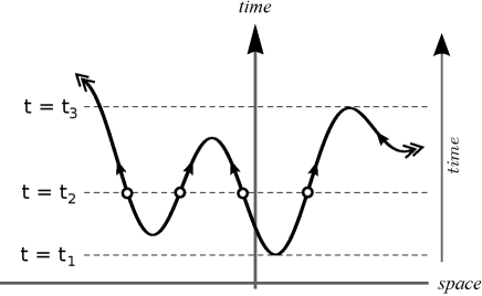
Figure 1: Generic worldline, numerous pointlike ‘‘particles’’ (at $t=t_{2}$) and creation (at $t=t_{1}$) or annihilation (at $t=t_{3}$) events

If, in the course of time, the parameter $t$ is assumed to increase monotonically, then a pair of particles can appear at a particular instant $t=t_{1}$ (or disappear at $t=t_{3}$). These ‘‘events’’ model the processes of creation (annihilation) of a pair ‘‘particle-antiparticle’’.

In the paper [Khasanov], we restricted our consideration to the plane (2D) motions and a polynomial form of the generating functions $\{F_{a}\}$ in (1). The latter restriction allows for a complete determination of the full set of roots-particles of the system and explicitly reveals the correlations in their positions and dynamics represented by the well-known Vieta formulas. Moreover, in a special ‘‘inertial-like’’ reference frame, the first (linear in roots) Vieta formula implies the conservation law for total momentum of the set of pointlike particles identified with the roots of (1). In this way one reproduces the general structure of Newtonian mechanics which, thus, turns out to be encoded in the algebraic properties of an arbitrary (implicitly defined) worldline! The most important results and ideas of the paper [Khasanov] are presented in section 2.

Apart of the obvious program of relativistic invariant formulation of the scheme (for this, see discussion in [Khasanov], section 5), there is a number of problems which can be successfully considered in the framework of purely Galilean-Newtonian picture. One of these is the determination of the full set of conservation laws which follow from the structure of the nonlinear (i.e., of higher degree in roots) Vieta formulas. These issues are examined in section 3. The problem of conservation of total angular momentum is separately treated in the next section 4 and turns out to relate to the Vieta’s constraints as well. In this section we also present a typical example of the polynomial system that defines a self-consistent dynamics of a number of roots-particles subject to all three canonical-like conservation laws. Section 5 contains some concluding remarks and discussion.

Collective Algebraic Dynamics on an Implicitly Defined Worldline

Consider, for example [Khasanov], a simple algebraic system of polynomial equations selected quite randomly (yet of rather low degrees in the unknowns $x,y$ and the time-like parameter $t$):

$$\left\{\begin{array}[]{ll}F_{1}(x,y,t)=-2x^{3}+y^{3}+tx+ty+y+2=0,\\ F_{2}(x,y,t)=-x^{3}-2x^{2}y+t+3=0.\end{array}\right.$$ (2)

Eliminating $t$, one obtains the trajectory

$$x^{4}+3x^{3}y+2x^{2}y^{2}-2x^{3}+y^{3}-3x-2y+2=0$$ (3)

which consists of three disconnected components (fig. 2). Solving now the second equation with respect to $y$ and substituting the result in the first one, we obtain a 1D polynomial equation of the form

$$\left\{\begin{array}[]{ll}P(x,t)=-17x^{9}+(4t-4)x^{7}+(3t+25)x^{6}+(4t^{2}+16t+12)x^{4}+\\ +(-3t^{2}-18t-27)x^{3}+t^{3}+9t^{2}+27t+27=0.\end{array}\right.$$ (4)

It can then be proved (say, via the resultants’ techniques, see section 3) that there is an analogous condition for the unknown $y$, namely,

$$\left\{\begin{array}[]{llll}Q(y,t)=17y^{9}+(33t+35)y^{7}+(-6t+52)y^{6}+(15t^{2}+34t+19)y^{5}+\\ +(-16t^{2}+8t+40)y^{4}+(-t^{3}+11t^{2}+49t+113)y^{3}+\\ +(-18t^{3}-72t^{2}-50t-12)y^{2}+(28t^{3}+148t^{2}+208t+48)y+\\ +t^{4}-48t^{2}-5t^{3}-96t-64=0.\end{array}\right.$$ (5)

For any value of the time-like parameter $t$ equation (4) has nine solutions $x_{k},\leavevmode\nobreak\ k=1,\ldots,9$, each one of which is in correspondence with a solution $y_{k}$ of (5) so that the pairs compose exactly nine solutions of the system (2). Some of these are real-valued, correspond to the so-called R-particles and belong to one of the three branches of the trajectory (3) while others arise as complex conjugate pairs and should be treated as another kind of composite particle-like formations, the so-called C-particles [Khasanov]. The latter can be visualized via equal real parts of complex conjugate roots and are located in the space off the trajectory (3), see fig.2.

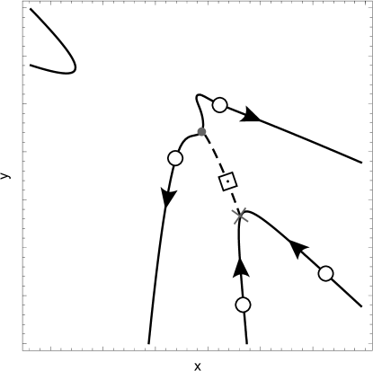
Figure 2: Three branches of the trajectory of R-particles and the typical succession of events (annihilation – propagation of a C-particle — creation)

At particular values of the time-like parameter $t$ defined by the condition (we rename here $x_{1}=x,\leavevmode\nobreak\ x_{2}=y$)

$$\det\left\|\frac{\partial F_{A}}{\partial x_{B}}\right\|=0,\quad A,B,\ldots=1,2,$$ (6)

some two real roots of the system (2) merge together and transform then into a complex conjugate pair or vice versa. These events can be evidently interpreted as the processes of annihilation of a pair particle-antiparticle accompanied by the formation of a ‘‘C-quantum’’, or creation of a pair, respectively. A typical succession of processes is represented at fig. 2. Note that, in contrast to the picture earlier suggested by Stueckelberg, all these processes necessarily satisfy a number of conservation laws, see below.

Consider now the set of Vieta formulas specific, say, for the polynomial equations (4,5) and explicitly representing the correlations in positions and dynamics of different particles-roots defined by the generating system (2). The first two of them (of lowest degrees in roots) have the following form:

$$x_{1}+x_{2}+\ldots+x_{9}=0,\quad y_{1}+y_{2}+\ldots+y_{9}=0;$$ (7)

and, respectively,

$$x_{1}x_{2}+x_{1}x_{3}+\ldots+x_{8}x_{9}=-\frac{1}{17}(4t-4),\leavevmode\nobreak\ \leavevmode\nobreak\ \\ y_{1}y_{2}+y_{1}y_{3}+\ldots+y_{8}y_{9}=\frac{1}{17}(33t+35),$$ (8)

where all the roots depend on $t$ and the zeros on the right-hand side of equations (7) are direct consequences of the absence of the 8-th degree terms in $P(x,t)$ and $Q(x,t)$, see (4,5). Recall now that for a mechanical system of nine particles with masses ${m_{k}}$ the coordinates of its center of mass are

$$X(t)=\frac{1}{9}(m_{1}x_{1}+\ldots+m_{9}x_{9}),\quad Y(t)=\frac{1}{9}(m_{1}y_{1}+\ldots+m_{9}y_{9}).$$ (9)

From the linear Vieta formulas (7) we conclude, therefore, that for the polynomial system (2) that defines the ensemble of nine particles of equal masses , the center of mass is at rest. Repeatedly differentiating then equations (7) with respect to the time-like parameter $t$, one obtains for instantaneous velocities $\{\vec{v}_{k}(t)\}$ and accelerations $\{\vec{a}_{k}(t)\}$ of the roots-particles:

$${\vec{v}}_{1}+{\vec{v}}_{2}+\ldots+{\vec{v}}_{9}=0,$$ (10)

and

$${\vec{a}}_{1}+{\vec{a}}_{2}+\ldots+{\vec{a}}_{9}=0.$$ (11)

Equation (10) demonstrates that the total momentum of nine particles of the ensemble is conserved and, precisely, equal to zero. As for the equation (11), one can identify the acceleration $\vec{a}_{k}$ with the resulting force $\vec{F}_{k}$ acting on the particle (of unit mass, $m_{k}=m=1$) from all other particles of the ensemble . Now one can say that equation (11) represents in fact the ‘‘weakened’’ form of the Newton’s third law: the sum of all resulting forces acting on all the nine particles in the ensemble is identically zero. Note that the velocities (momenta), accelerations and other physical quantities of C-particles can be always considered real-valued since they correspond to complex conjugate pairs of roots, so that their imaginary parts cancel and do not enter the constraints (10,11).

Let us examine now the next, quadratic in roots, Vieta formulas (8). It is easy to see that, making use of the linear formulas (7), the former can be equivalently rewritten for the sums of squares of the roots as follows:

$$x_{1}^{2}+x_{2}^{2}+\ldots+x_{9}^{2}=\frac{2}{17}(4t-4),\quad y_{1}^{2}+y_{2}^{2}+\ldots+y_{9}^{2}=-\frac{2}{17}(33t+35).$$ (12)

Composing now a $SO(2)$-invariant combination of the two equations (12) (which only is coordinate-independent and thus physically meaningful), one obtains:

$$r_{1}^{2}+r_{2}^{2}+\ldots+r_{9}^{2}=-(58/17)t-(78/17),$$ (13)

where $r_{k}^{2}:=x_{k}^{2}+y_{k}^{2}$. Note that the left-hand side of the equation (13) is real but not positive definite since some roots are complex conjugate. The obtained formula (13), though interesting, is in fact accidental: we shall see below (section 3) that, generally, the dependence on the time-like parameter $t$ in the right-hand side of equations like (13) is rather quadratic than linear. That is why, to obtain a physically valuable conservation law, one has to differentiate it twice. It follows then:

$$(v_{1}^{2}+v_{2}^{2}+\ldots+v_{9}^{2})+({\vec{a}}_{1}{\vec{r}}_{1}+{\vec{a}}_{2}{\vec{r}}_{2}+\ldots+{\vec{a}}_{9}{\vec{r}}_{9})=const=0.$$ (14)

The first group of terms reproduces the (doubled) total kinetic energy whereas the second group stands for the analogue of potential energy (or, more closely, total amount of work of all the resulting forces). Thus, we obtain a coordinate-free constraint which strongly resembles the law of mechanical energy conservation  but obviously has a different form! Nonetheless, the correlated dynamics of particles defined by the systems like (2) is governed not only by the law of conservation of total momentum but by the energy-like conservation law (14) as well!

It is also noteworthy that the equality

$$\frac{d}{dt}(\frac{1}{2}v_{k}^{2})\equiv\vec{a}_{k}\vec{v}_{k}\equiv\vec{F}_{k}\vec{v}_{k}$$ (15)

is in fact the well-known balance equation for kinetic energy which does not depend on the particular form of interaction and is valid identically under the identification of acceleration $\vec{a}_{k}$ with the resulting force $\vec{F}_{k}$.

Let us further examine the situation with angular momentum vector

$$\vec{M}=\sum\vec{M}_{k},\quad M_{k}:=\vec{r}_{k}\times\vec{v}_{k},$$ (16)

which for the considered case of a plane motion has only one nontrivial component. The procedure of analytic determination of the latter will be described in section 4 while at the moment we only announce that for a very wide class of generating polynomial systems like (2) the total angular momentum is also conserved. In particular, for the considered system of equations (2) it is precisely zero! Of course, this result can be confirmed by direct numerical calculations.

We can now conclude that the (randomly chosen!) system (2), without any appeal to the Newton’s laws or some other differential equations of motion, completely defines a self-consistent (algebraic in nature) dynamics of the ensemble of (two kinds of) particles. This dynamics is subject to a number of conservation laws (reproducing, in most part, the canonical set of these), includes mutual transmutations of particles, etc. The detailed analysis and full animation of such, unexpectedly rich dynamics (in which, however, one had not considered the angular momentum and the energy-like conservation laws) was presented in the previous paper [Khasanov].

Quite naturally, a number of remarkable problems arise at the moment: to what extent is the situation represented by the particular system (2) typical? How wide is the class of polynomial (or even general algebraic) systems of equations which ensure the validity of conservation laws? Does there exist an exceptional algebraic system (or a class of these) that completely reproduces the Newtonian dynamics, and to what kind of particle interaction it corresponds then? What changes will occur during the 3D generalization of the presented scheme? In which way one can adapt the construction to the requirements of Special Relativity? At least first two of these problems will be examined and partially solved below.

Vieta Formulas Generate Conservation Laws

Consider the general 2D situation when a system of two polynomial equations

$$\left\{\begin{array}[]{llll}F_{1}(x,y,t)=[a_{n,0}(t)x^{n}+a_{n-1,1}(t)x^{n-1}y+...+a_{0,n}(t)y^{n}]+...\\ \leavevmode\nobreak\ \leavevmode\nobreak\ \leavevmode\nobreak\ \leavevmode\nobreak\ \leavevmode\nobreak\ \leavevmode\nobreak\ \leavevmode\nobreak\ \leavevmode\nobreak\ \leavevmode\nobreak\ \leavevmode\nobreak\ \leavevmode\nobreak\ \leavevmode\nobreak\ \leavevmode\nobreak\ \leavevmode\nobreak\ \leavevmode\nobreak\ \leavevmode\nobreak\ \leavevmode\nobreak\ \leavevmode\nobreak\ +a_{0,0}(t)=0,\\ F_{2}(x,y,t)=[b_{m,0}(t)x^{m}+b_{m-1,1}(t)x^{m-1}y+...+b_{0,m}(t)y^{m}]+...\\ \leavevmode\nobreak\ \leavevmode\nobreak\ \leavevmode\nobreak\ \leavevmode\nobreak\ \leavevmode\nobreak\ \leavevmode\nobreak\ \leavevmode\nobreak\ \leavevmode\nobreak\ \leavevmode\nobreak\ \leavevmode\nobreak\ \leavevmode\nobreak\ \leavevmode\nobreak\ \leavevmode\nobreak\ \leavevmode\nobreak\ \leavevmode\nobreak\ \leavevmode\nobreak\ \leavevmode\nobreak\ \leavevmode\nobreak\ +b_{0,0}(t)=0\end{array}\right.$$ (17)

is under investigation. Note that only forms of the highest ($n$ and $m$, respectively) and the least orders are written out in (17). The coefficients $\{a_{i,j}(t),b_{i,j}(t)\}$ depend on the evolution time-like parameter $t$ and take values in the field of real numbers $\mathbb{R}$.

All the roots $\{x_{0}(t),y_{0}(t)\}$ of such a system are either real or entering both in complex conjugate pairs. In order to find all the roots of the system (17), one must somehow eliminate one of the unknowns, say $x$, reduce the system to a 1D polynomial equation in $y$, with coefficients depending on $t$, and make then use of the fundamental theorem of algebra. The procedure can be accomplished by making use of the so-called method of resultants (see, e.g., [Gelfand, Morozov] and our paper [Khasanov]). As a rule , the resulting polynomial will be of degree $N=nm$, and the sought for equation has the form

$$R_{x}(y)=g_{N}(t)y^{N}+g_{N-1}(t)y^{N-1}+\ldots+g_{0}(t)=0.$$ (18)

The structure of the resultant (which in this case is often called eliminant) is represented by the determinant of the Sylvester matrix (see, e.g., [Morozov, Prasolov]). The coefficients $\{g_{I}(t)\}$ depend on $\{a_{i,j}(t),b_{i,j}(t)\}$. One can exchange the coordinates, and after the elimination of $y$ arrive at the dual condition

$$R_{y}(x)=f_{N}(t)x^{N}+f_{N-1}(t)x^{N-1}+\ldots+f_{0}(t)=0.$$ (19)

Note that, generally, the degrees of $R_{x}(y)$ and $R_{y}(x)$ eliminants are the same and equal to $N=nm$ (see, for details, [Khasanov], section 3). Of course, in the case of a rather great $N$, algebraic computer programs should be used to find the explicit form of eliminants. Then, for any value of $t$, all the $N$ solutions of (18) and (19) over $\mathbb{C}$ can be (numerically) evaluated and put in correspondence to each other to obtain $N$ solutions $\{x_{k}(t),y_{k}(t)\},k=1,2,..N$ of the initial system (17).

Since any system of two polynomial equations can be reduced to a pair of dual equations (18) and (19) for eliminants, polynomials in one variable each, the well-known Vieta formulas are in fact applicable in the 2D case under consideration. Specifically, one has the following system connecting all the roots of (19) or (18):

$$\begin{array}[]{llll}\Sigma x_{k}=-f_{N-1}(t)/f_{N}(t),\leavevmode\nobreak\ \leavevmode\nobreak\ \Sigma y_{k}=-g_{N-1}(t)/g_{N}(t),\nobreak\leavevmode\nobreak\leavevmode\\ \Sigma x_{i}x_{j}=f_{N-2}/f_{N}(t),\leavevmode\nobreak\ \leavevmode\nobreak\ \Sigma y_{i}y_{j}=g_{N-2}/g_{N}(t),\nobreak\leavevmode\nobreak\leavevmode\\ .............................................................................................\\ x_{1}x_{2}...x_{N}=(-1)^{N}f_{0}(t)/f_{N}(t),\leavevmode\nobreak\ \leavevmode\nobreak\ y_{1}y_{2}...y_{N}=(-1)^{N}g_{0}(t)/g_{N}(t)\end{array}$$ (20)

(summation over all the roots with $k=1,2,..N$,   $i,j=1,2,..N,\leavevmode\nobreak\ \leavevmode\nobreak\ i<j,\leavevmode\nobreak\ \ldots$, is accepted above and throughout the paper).

Let us suppose now that the coefficients of the general polynomial system (17) are also polynomials with respect to the time-like parameter $t$. If the latter is considered on the same foot as the coordinates $x,y$, one can easily see that, in the general ‘‘nondegenerate’’ case (see below), the coefficients in the higher degree monomials $a_{n,0},a_{n-1,1},\ldots a_{0,n}$ and $b_{m,0},b_{m-1,1},\ldots b_{0,m}$ do not depend on time at all, the coefficients in the next, lower order monomials depend on $t$ linearly, and so on.

Further, during the procedure of elimination, say of $x$, the property of homogeneity of corresponding sums of the monomials of the same degree in the eliminant $R_{x}(y,t)$ with respect to $y$ and $t$ will be evidently preserved. This is equivalent to the statement that the coefficients $g_{N}$, $g_{N-1}$, $g_{N-2}$, …will be of order $0,1,2,\ldots$ in $t$, respectively. The same can be certainly said about the coefficients $f_{N}\sim t^{0},\leavevmode\nobreak\ f_{N-1}\sim t^{1},\leavevmode\nobreak\ f_{N-2}\sim t^{2},\ldots$ in $R_{y}(x)$.

In particular, the coefficients $g_{N},f_{N}$ in the leading terms of the eliminants depend only on the corresponding coefficients in the leading monomials  [Brill, Utyashev] and are, therefore, constants in the case under consideration. The exact connection of these coefficients had been computed in [Brill, Utyashev] and, generally, is of the following form:

$$g_{N}\equiv f_{N}={\mathrm{Res}}[F_{1}^{(n)}(\xi,1)],F_{2}^{(m)}(\xi,1),\xi]\equiv{\mathrm{Res}}[F_{1}^{(n)}(1,\xi),F_{2}^{(m)}(1,\xi),\xi],$$ (21)

where $F_{1}^{(n)}(x,y),\leavevmode\nobreak\ F_{2}^{(m)}(x,y)$ are the sums of the leading monomials, of degrees $n$ and $m$ respectively, of the generating polynomials in (17), and $Res[..]$ designates corresponding resultant of these two over $\xi$, under the substitution $x=\xi,\leavevmode\nobreak\ y=1$ or, equivalently, $x=1,\leavevmode\nobreak\ y=\xi$. Below we assume that the principal coefficients (21) are nonzero. The illustration of the above described construction will be presented in section 4.

Let us now look once more at the Vieta formulas (20). The right-hand sides of formulas of the $I$-th order in roots are proved to be polynomials of the $I$-th degree in $t$. Therefore, after $I$ differentiations by $t$ of the corresponding formula, one necessarily arrives at a constant in the right-hand side of the final equation. This means that there exists a whole set of time-independent relations (constraints) between the positions, velocities, accelerations, etc. of the particles-roots!

On the other hand, the canonical representation of conservation laws has the form of a sum of various characteristics of individual particles. In order to obtain such a form from the above established relations, let us make use of the so-called Newton’s identities [NewtonId] which easily allow to express the left-hand sides of (20) as the sums of $I$-th degrees of the roots $\{x_{k}\}$ or $\{y_{k}\}$, respectively. As a result, one obtains the following formulas establishing dynamical correlations between the roots-particles of the generating system (17):

$$\begin{array}[]{llll}\Sigma x_{k}=A_{1}(t),\leavevmode\nobreak\ \leavevmode\nobreak\ \Sigma y_{k}=B_{1}(t),\nobreak\leavevmode\nobreak\leavevmode\\ \Sigma x_{k}^{2}=A_{2}(t),\leavevmode\nobreak\ \leavevmode\nobreak\ \Sigma y_{k}^{2}=B_{2}(t),\nobreak\leavevmode\nobreak\leavevmode\\ .........................................\\ \Sigma x_{k}^{N}=A_{N}(t),\leavevmode\nobreak\ \leavevmode\nobreak\ \Sigma y_{k}^{N}=B_{N}(t),\end{array}$$ (22)

where $A_{k}(t)$, $B_{k}(t)$ are some polynomials in $t$ of degree $k$, respectively.

Now again one can differentiate by $t$ each of the modified Vieta formulas (22) appropriate number of times to obtain a constant in its right-hand side. In this way one evidently comes to a chain of conservation relations which contain the sums of combinations of the roots, separately of $\{x_{k}\}$ and $\{y_{k}\}$, and their higher order time derivatives and do hold for any generating system of equations (17), under the above described, quite general polynomial dependence of the coefficients on time $t$. Thus, any system of two nondegenerate polynomial equations in $x,y,t$ defines a collective dynamics of $N=nm$ particles-roots for which a set of $2(N-1)$ conservation laws does exist!

Consider now in more detail the first two modified Vieta formulas which in fact we have already dealt with in the previous section. Simplest, linear in roots, Vieta formulas in (22) represent the dynamics of the center of mass of a system of $N$ identical particles-roots, with coordinates

$$X(t)=\frac{1}{N}\sum x_{k},\quad Y(t)=\frac{1}{N}\sum y_{k},$$ (23)

and asserts (due to linear dependence of $A_{1},\leavevmode\nobreak\ B_{1}$ on time $t$) that the center of mass always moves uniformly and rectilinearly, in full correspondence with the usual Newtonian mechanics. After first and second differentiation by $t$, one obtains then the law of conservation of total momentum and the ‘‘weakened’’ form of the Newton’s third law; compare this with the example in the previous section 2.

As for the next, quadratic in roots, formulas in (22), their right-hand sides also depend on $t$ quadratically. That’s why, to obtain a corresponding conservation law, one has to differentiate them twice and to compose then a $SO(2)$-invariant combination of the resulting equations for $x$ and $y$ parts. Then, as it was already demonstrated at the example in section 2, one comes to the conservation law for the analogue of total mechanical energy:

$$\Sigma v_{k}^{2}+\Sigma{\vec{a}}_{k}{\vec{r}}_{k}=const.$$ (24)

Both terms in (24) are real-valued, despite the contribution of complex conjugate pairs of roots. However, imaginary parts of the latter contribute to the sums; in particular, the first term is not positively definite, since $\Re(v_{k}^{2})=\Re(v_{k})^{2}-\Im(v_{k})^{2}$. Thus, the first term corresponds to the (doubled) total kinetic energy when only contributions from the $C$-particles related to complex conjugate pairs of roots can be neglected. Generally, one should take into account another sort of ‘‘kinetic’’ energy which is negative; its physical meaning, as well as of the second term standing in place of the potential energy, at present is vague.

In this connection, nonetheless, it should be noted that the conservation law (24) is also tightly connected with the well-known virial theorem from the classical mechanics (see, e.g., [Golstein, p.83]). However, the latter corresponds to the null constant in the right-hand side and, besides, holds only in average for finite movements whereas the constraint (24) is satisfied at any instant. Remarkably, for potential forces homegeneous with respect to the mutual distances $r_{ij}$ (so that the pairwise potential energies $U_{ij}\propto r_{ij}^{n},\leavevmode\nobreak\ \leavevmode\nobreak\ n\in\mathbb{Z}$) the second term in (24) is equal to $-nU$, where $U$ is the total potential energy [Golstein, p.86]. Thus, just in the case $n=-2$ the constraint (24) exactly reproduces the canonical form of the energy conservation law. That is, the interaction of the form $U\propto 1/r^{2}$ is, though implicitly, distinguished among others in the framework of ‘‘polynomial mechanics’’. We recall, however, that, in the construction under consideration, possibility of the decomposition of the resultant forces (=accelerations) into the pairwise (radial) constituents is not yet proved if possible.

Finally, let us consider the Vieta formulas (22) of higher orders in roots. The constraints for time derivatives of corresponding order from the higher order sums $\sum x_{k}^{3},\sum y_{k}^{3},\ldots,\sum x_{k}^{N},\sum y_{k}^{N}$ will evidently result in the whole set of (non-canonical) conservation laws. However, these constraints do not allow for $SO(2)$-invariant (generally, $SO(3)$-invariant) combinations and are, therefore, coordinate dependent and, most likely, not physically valuable. Nonetheless, this problem certainly deserves further investigation.

The Law of Angular Momentum Conservation

We are now ready to consider the problem of conservation of the total angular momentum, the last of the set of rotation-invariant canonical conservation laws. In the 2D case there exists only one component of the angular momentum vector

$$M_{z}=\sum M_{k},\quad M_{k}:=x_{k}(v_{y})_{k}-y_{k}(v_{x})_{k}.$$ (25)

Instantaneous velocities $v_{x},v_{y}$ can be expressed through the coordinates $x,y$ and $t$. Specifically, differentiating by $t$ the equations (18, 19) for eliminants $R_{y}(x,t)$ and $R_{x}(y,t)$, one easily finds:

$$v_{x}(t)=-\frac{\partial_{t}R_{y}(x,t)}{\partial_{x}R_{y}(x,t)},\quad v_{y}(t)=-\frac{\partial_{t}R_{x}(y,t)}{\partial_{y}R_{x}(y,t)},$$ (26)

so that one obtains the desired expression for angular momentum. Composing now the auxiliary function

$$H(M,x,y,t):=M-(xv_{y}-yv_{x}),$$ (27)

reducing it to common denominator and equating then the numerator to zero, one arrives at the additional polynomial equation of the form

$$M\partial_{y}R_{x}(y)\partial_{x}R_{y}(x)+x\partial_{t}R_{x}(y)\partial_{x}R_{y}(x)-y\partial_{t}R_{y}(x)\partial_{y}R_{x}(y)=0.$$ (28)

Together with the generating equations (17) themselves, equation (28) constitute a complete system of three polynomial equations for determination of the values of angular momenta and their temporal dependence of all the particles-roots. For this, we must successfully eliminate both $x$ and $y$, again making use of the resultants’ techniques, and arrive at a polynomial equation of the form $F(M,t)=0$. As a rule, it consists of two multipliers from which only one corresponds to the true solutions of the system under consideration whereas the second factor leads to the redundant solutions . Separating the proper factor (which should be exactly of the degree $N=nm$) and making then use of the linear Vieta formula, one obtains the value of total angular momentum $M_{z}$ and verifies that it is always time independent!

Let us now illustrate the above-presented procedure at a typical example of a system of two independent and nondegenerate polynomial (with respect to both $x,y$ and $t$) equations of the degrees $n=3$ and $m=2$, respectively, with arbitrary chosen (integer) real-valued coefficients. Specifically, let us take

$$\begin{array}[]{llll}F_{1}=(3x^{3}+7y^{3}+6t^{3}-2x^{2}y+5xy^{2}+7t^{2}x-4t^{2}y\\ \leavevmode\nobreak\ \leavevmode\nobreak\ \leavevmode\nobreak\ +6tx^{2}-5ty^{2}-9xyt)+(-x^{2}-3y^{2}-9t^{2}-xy-10tx-11ty)\\ \leavevmode\nobreak\ \leavevmode\nobreak\ \leavevmode\nobreak\ +(3x+2y-13t)-8=0,\\ F_{2}=(7x^{2}-12y^{2}-4t^{2}+17xy+5tx-11ty)\\ \leavevmode\nobreak\ \leavevmode\nobreak\ \leavevmode\nobreak\ +(19x+21y+3t)+1=0.\end{array}$$ (29)

Let us now rewrite the above system in the following equivalent form. Collecting the monomials in $x$ and $y$ and fixing in this way the coefficients in their terms depending on $t$, one obtains the sought for structure of the generating system (29):

$$\begin{array}[]{llll}F_{1}=(3x^{3}-2x^{2}y+5xy^{2}+7y^{3})+(6t-1)x^{2}-(9t+1)xy-\\ \leavevmode\nobreak\ \leavevmode\nobreak\ \leavevmode\nobreak\ \leavevmode\nobreak\ \leavevmode\nobreak\ \leavevmode\nobreak\ \leavevmode\nobreak\ \leavevmode\nobreak\ (5t+3)y^{2}+(7t^{2}-10t+3)x-(4t^{2}+11t-2)y+\\ \leavevmode\nobreak\ \leavevmode\nobreak\ \leavevmode\nobreak\ \leavevmode\nobreak\ \leavevmode\nobreak\ \leavevmode\nobreak\ \leavevmode\nobreak\ \leavevmode\nobreak\ (6t^{3}-9t^{2}-13t-8)=0,\nobreak\leavevmode\nobreak\leavevmode\\ F_{2}=(7x^{2}+17xy-12y^{2})+(5t+19)x-(11t-21)y-\\ \leavevmode\nobreak\ \leavevmode\nobreak\ \leavevmode\nobreak\ \leavevmode\nobreak\ \leavevmode\nobreak\ \leavevmode\nobreak\ \leavevmode\nobreak\ \leavevmode\nobreak\ (4t^{2}-3t-1)=0.\end{array}$$ (30)

Thus, we see (cf. with the statement on page 8) that the coefficients in the monomials of $(n-I)$-th or $(m-I)$-th degree in $x,y$, respectively, are polynomials in $t$ of the $I$-th degree.

Taking now the resultant of $F_{1}$ and $F_{2}$ over $y$ and under fixed $x$, one obtains the eliminant equation of the form

$$\begin{array}[]{lll}R_{y}(x,t)=-358343x^{6}+(-374447t-1176858)x^{5}+\\ \left(103876t^{2}-864563t-1155352\right)x^{4}+...\\ +(-111802t^{6}-112903t^{5}+...+370780)=0,\end{array}$$ (31)

and, acting in full analogy, the dual equation

$$\begin{array}[]{lll}R_{x}(y,t)=-358343y^{6}+(145966t-95313)y^{5}+\\ \left(2828t^{2}+968047t-354945\right)y^{4}+...\\ +(4148t^{6}-40308t^{5}+...+222804)=0.\end{array}$$ (32)

Again, the coefficients in the terms of $(N-I)$-th degree (with $N=6$) in the eliminants (31,32) are polynomials in $t$ of the $I$-th degree (cf., once more, with the corresponding statement on page 8). In particular, both leading coefficients in the eliminants $f_{6}=g_{6}=-358343$ are equal and can be equivalently computed via formula (21). They do not turn to zero so that the system (29) is indeed nondegenerate.

Thus, we can presuppose that this system, of a quite general form, uniquely defines the correlated dynamics of $N=3\times 2=6$ particles of equal masses (some of which being merged into complex conjugate pairs and possessing, therefore, a twice greater mass) for which the laws of conservation of total momentum, total angular momentum and the analogue of total mechanical energy are valid all three together!

At any $t$, equations (31) and (32) both have 6 solutions some of them being real and some entering in complex conjugate pairs. Putting these in correspondence to each other, one obtains all 6 solutions of the generating system (30). Further, the discriminants of the eliminants (31) and (32) contain a common factor $D(t)$ which is a polynomial in $t$ of the order 18 and turns to zero at 18 values of $t$; however, only 2 of them are real. Thus, there are precisely 2 instants at which some two of the roots of (30) become multiple; physically, these correspond to the ‘‘events’’ of annihilation of a pair of $R$-particles or, conversely, creation of a pair from a composite $C$-particle.

Making use of the linear Vieta formulas for (31) and (32), one immediately finds that the center of mass of the ‘‘closed mechanical system’’ of 6 particles moves uniformly with the (dimensionless) velocity ${\vec{V}}=\{V_{x},V_{y}\},\leavevmode\nobreak\ \leavevmode\nobreak\ V_{x}=-374447/358343,\leavevmode\nobreak\ V_{y}=145966/358343$.

From the second order (modified) Vieta formulas for $x$ and $y$ parts one finds after two differentiations by $t$ and summation of both:

$$(v_{1}^{2}+\ldots+v_{6}^{2})+(\vec{a}_{1}\vec{r}_{1}+\ldots+\vec{a}_{6}\vec{r}_{6})=const=\frac{237989891909}{358343^{2}}\approx 1.85336.$$ (33)

Calculating now the expression for numerator of the defining function of angular momentum (27), one obtains the (rather complicated) polynomial equation of the form (28),

$$\Phi(M,x,y,t)=0.$$ (34)

Eliminating successively $x$ and $y$ from the joint system of equations (30) and (34), via calculating corresponding resultants, one arrives at the polynomial equation for angular momenta of the particles that turns out to be of the form $F(M,t)G(M,t)=0$, with $F$ and $G$ being polynomials in $M$ of degrees 90 (!) and 6, respectively. So it is evident (and can be verified through numerical calculations of the roots and related angular momenta) that the first factor leads to redundant solutions whereas the equation

$$G(M,t)=\alpha(t)M^{6}+\beta(t)M^{5}+\gamma(t)M^{4}+\ldots+\varepsilon(t)=0$$ (35)

properly defines the values of angular momenta of all 6 particles at any instant of time! In (35) the coefficients $\alpha(t)=358343A(t)$ and $\beta(t)=827188A(t)$ turn out to be proportional to each other by the factor $A(t)=A_{0}t^{18}+A_{1}t^{17}+...+A_{18}$ which is a polynomial   of 18-th degree in $t$ with very large integer numerical coefficients $\{A_{j}\},\leavevmode\nobreak\ j=1,..18$. Now, making use of the linear Vieta formula for the equation (35), one immediately obtains the value of total angular momentum of 6 particles:

$$M_{z}=\sum M_{k}=-\frac{\beta(t)}{\alpha(t)}=const=-\frac{827188}{358343}\approx-2.308$$ (36)

which, remarkably, does not depend on $t$! Of course, this result had been also reproduced via direct numerical calculations under numerous values of the time parameter $t$. Considerable number of other examples of the algebraic systems of equations with nondegenerate polynomials in $x,y$ and $t$, of different and rather high degrees (say, $n=7,\leavevmode\nobreak\ m=5$) had been studied; for all the examples three canonical-like conservation laws are undoubtedly satisfied, and the corresponding physical characteristics were exactly computed.

Conclusion

In the paper we have demonstrated that for a very wide class of systems of polynomial equations, with polynomial dependence of the (real-valued) coefficients on the time parameter, there exists a whole set of time-independent constraints on the roots of the system and their time derivatives. Real roots can be identified with one sort (R-) of identical particlelike formations while complex conjugate with the other one, C-particles, possessing a twice greater mass and participating in the processes of annihilation or creation of a pair of R-particles.

Thus, one gets a nontrivial correlated (at present, 2D nonrelativistic) dynamics of the ensemble of R- and C-particles. This can model real physical dynamics in a system of interacting particles and even replace its canonical description on the base of the Newton’s differential equations of motion.

Time-independent constraints arising in our scheme are generated by the set of the Vieta formulas that impose rigid restrictions on the instantaneous positions of particles-roots, their velocities, accelerations, etc. We have shown that, generally, these constraints can be transformed into the form of conservation laws. Moreover, all the canonical rotation-invariant conservation laws are represented herein. In particular, for any nondegenerate polynomial (with respect both to $x,y$ and $t$) system of equations the laws of conservation of total momentum, angular momentum and (the analogue of) total mechanical energy are satisfied!

In the framework of the concept of the ‘‘unique worldline’’, there are a lot of both mathematical and physical problems to be solved. As for mathematics, one has every reason to think that a sort of generalized Vieta-like formulas relating different roots of any system of two or more polynomial equations do exist and could be discovered; this is an interesting challenge for ‘‘pure’’ mathematicians. In particular, such formulas, in contrast with the familiar 1D case, could explicitly mix different coordinates $x,y,\ldots$ of the solutions and, under the presence of the time-like parameter, their time derivatives. These conjectural relations would help to explain, say, the effect of angular momentum conservation which at present is confirmed only on an essential number of examples but not in a general analytical form .

As for physics (which is also completely induced herein by the purely mathematical properties of polynomials), one should generalize the scheme to the physical 3D case and find the road to the relativistic reformulation of the theory. Apart of these obvious goals, the problem of determination of an effective pairwise particle interaction’ force is on the agenda. And, of course, one should analyze the meaning of the term which stands for the ordinary potential energy in the corresponding conservation law (24). The principal question is, however, the following: is it possible to form composite and stable multi-particle clusters modelling the real elementary particles, nuclei, etc. from the initial R- and C- pre-elements of matter naturally arising in our scheme? And how could be then interpreted the latter from the physical viewpoint?

In general, there are a lot of remarkable relations in mathematics, and in the nonlinear algebra in particular [Morozov2], which are not yet discovered but could be responsible for the structure of fundamental physical laws. Here we have undertaken one more attempt  to shed some light upon the deep connections existing between fundamental physics and mathematics.

References

- [1] Stueckelberg, E. C. G. Remarque á propos de la crèation de paires de particules en théorie de relativitè. Helv. Phys. Acta, 14:588–594, 1941.
- [2] Stueckelberg, E. C. G. La mécanique du point matériel en théorie de relativité et en théorie des quants. Helv. Phys. Acta, 15:23–37, 1942.
- [3] Feynman, R. P. The development of the space-time view of quantum electrodynamics. Science, 153:699–708, 1966.
- [4] Feynman, R. P. The theory of positrons. Phys. Rev., 76:749–759, 1949.
- [5] Kassandrov, V. V. and Khasanov, I. Sh. Algebraic roots of Newtonian mechanics: correlated dynamics of particles on a unique worldline. J. Phys. A: Math. Theor., 46:175–206, 2013. (arXiv:1211.7002 [physics.gen-ph]).
- [6] Gelfand, I. M., Kapranov, M. M. and Zelvinsky, A. V. Discriminants, Resultants and Multidimensional Determinants. Birkhäuser, Boston, 2008.
- [7] Morozov, A. Yu. and Shakirov, R. Sh. New and Old Results in Resultant Theory. Theor. and Math. Physics, 163:587–617, 2010. (arXiv:0911.5278 [math-ph]).
- [8] Prasolov, V. V. Polynomials. Springer, Berlin, 2004.
- [9] von Brill, A. Vorlesungen über ebene algebraische kurven und algebraische funktionen. Druck und Verlag von Friedr. Vieweg & Sohn, Braunschweig, 1925.
- [10] Kalinina, E. A. and Utyashev, A. Yu. Exclusion theory. St.-Petersb. Univ. Press, Saint-Petersburg, 2002. (in Russian).
- [11] Mead, D.G. Newton’s Identities. The Am. Math. Monthly (Math. Assoc. of Am.), 99:749–751., 1992.
- [12] Goldstein, H., Poole, C. and Safko J. Classical mechanics. 3-d edition. Addison Wesley, 2007.
- [13] Dolotin, V. and Morozov, A. Introduction to Nonlinear Algebra. World Sci., Singapore, 2007. (arXiv:hep-th/0609022).
- [14] Kassandrov, V. V. Algebraic structure of space-time and algebrodynamics. Peoples’ Friend. Univ. Press, Moscow, 1992. (in Russian).
- [15] Kassandrov, V. V. Algebrodynamics over complex space and phase extension of the Minkowski geometry. Phys. Atom. Nuclei, 72:813–827, 2009. (arXiv:0907.5425 [physics.gen-ph]).