Screening properties of four mesoscale smoothed charge models,
with application to dissipative particle dynamics

Abstract

We extend our previous study [J. Chem. Phys. 138, 204907 (2013)] to quantify the screening properties of four mesoscale smoothed charge models used in dissipative particle dynamics. Using a combination of the hypernetted chain integral equation closure and the random phase approximation, we identify regions where the models exhibit a real-valued screening length, and the extent to which this agrees with the Debye length in the physical system. We find that the second moment of the smoothed charge distribution is a good predictor of this behaviour. We are thus able to recommend a consistent set of parameters for the models.

I Introduction

Dissipative particle dynamics (DPD) has attracted much interest as a simulation method for soft condensed matter, including charged systems such as ionic surfactants and water-soluble polyelectrolytes which are of widespread practical importance Frenkel and Smit (2002); Noro et al. (2003); Groot (2003). In such systems, modelling the electrostatic interactions can be done implicitly, for example with the Poisson-Boltzmann equation, or explictly by incorporating charged particles. In the latter case, in DPD it is essential to smooth the point charges into charge clouds since this replaces the $1/r$ divergence of the Coulomb law as $r\to 0$ (where $r$ is the center-center separation) by a smooth cutoff, thus ensuring thermodynamic stability according to a theorem by Fisher and Ruelle Fisher and Ruelle (1966).

The precise form of the charge smoothing is often tuned to the choice of numerical algorithm and a consensus on the best approach has yet to emerge. At least four different smoothing methods have been suggested in the literature. Groot introduced a particle-particle particle-mesh (P³M) method with linear charge smoothing Groot (2003). Later González-Melchor et al. examined an Ewald-based method with exponential charge smoothing González-Melchor et al. (2006). Most recently we have studied a related Ewald method with Gaussian charge smoothing Warren et al. (2013). This last choice connects with recent work on the so-called ultrasoft restricted primitive model (URPM) Coslovich et al. (2011a, b); Nikoubashman et al. (2012). Finally, in the context of the URPM, a Bessel smoothed charge model has been introduced to complement the Gaussian case Warren and Masters (2013).

In the present work we extend the study in Ref. Warren et al., 2013 to identify regions where the models exhibit a real-valued screening length, and the extent to which this agrees between models and with the Debye length in the physical system. The problem will be addressed using liquid state integral equation theory Hansen and McDonald (2006). By focussing on the screening properties of the supporting electrolyte, we eliminate the need to consider explicit mesoscopic objects such as polymers and surfactants.

II Models

We first set out the generic DPD electrolyte model which underpins the rest of the discussion. More details and justification for particular parameter choices can be found in previous work Warren et al. (2013). We represent the electrolyte as a multicomponent soft sphere fluid of DPD particles, containing positive and negative ions of valencies $z_{\pm}$ at densities $\rho_{\pm}$, and a neutral ($z_{0}=0$) solvent species at a density $\rho_{0}$. The total ion density is $\rho_{z}=\rho_{+}+\rho_{-}$, and the total overall density is $\rho=\rho_{0}+\rho_{z}$; these are sufficient to specify the state point since charge neutrality implies $z_{+}\rho_{+}+z_{-}\rho_{-}=0$. The aforementioned charge clouds are centered on the DPD particles which represent the ions.

charge type	$\varrho(r)$	$g(k)=\tilde{\varrho}^{2}$	$f(r)$	$\beta u_{0}$	$\langle r^{2}\rangle$
linear	$\displaystyle\frac{3}{\pi R^{3}}\Bigl{(}1-\frac{r}{R}\Bigr{)}$	$\displaystyle\frac{144[2-2\cos(kR)-kR\sin(kR)]^{2}}{(kR)^{8}}$	—	$\displaystyle\frac{52\,l_{\mathrm{B}}}{35\,R}$	$\displaystyle\frac{2}{5}R^{2}$
exponential	$\displaystyle\frac{e^{-2r/\lambda}}{\pi\lambda^{3}}$	$\displaystyle\frac{1}{(1+{k^{2}\lambda^{2}}/{4})^{4}}$	$\displaystyle 1-e^{-2r/\lambda}\Bigl{(}1+\frac{11r}{8\lambda}+\frac{3r^{2}}{4\lambda^{2}}+\frac{r^{3}}{6\lambda^{3}}\Bigr{)}$	$\displaystyle\frac{5l_{\mathrm{B}}}{8\lambda}$	$\displaystyle 3\lambda^{2}$
Gaussian	$\displaystyle\frac{e^{-r^{2}/2\sigma^{2}}}{(2\pi\sigma^{2})^{3/2}}$	$\displaystyle{e^{-k^{2}\sigma^{2}}}$	$\displaystyle\operatorname{erf}\Bigl{(}\frac{r}{2\sigma}\Bigr{)}$	$\displaystyle\frac{l_{\mathrm{B}}}{\sigma\sqrt{\pi}}$	$\displaystyle 3\sigma^{2}$
Bessel	$\displaystyle\frac{1}{2\pi^{2}\sigma^{2}r}K_{1}\Bigl{(}\frac{r}{\sigma}\Bigr{)}$	$\displaystyle\frac{1}{1+k^{2}\sigma^{2}}$	$\displaystyle 1-e^{-r/\sigma}$	$\displaystyle\frac{l_{\mathrm{B}}}{\sigma}$	$\displaystyle 3\sigma^{2}$

Table 1: Properties of the four smoothed charge models: charge distribution $\varrho(r)$, auxiliary function $g(k)$, smoothing function $f(r)$ modifying the Coulomb law in Eq. (1), overlap energy $\beta u_{0}$, and second moment of charge distribution $\langle r^{2}\rangle$.

The fluid particles interact by pair-wise short range soft repulsions and long range electrostatics, with an interaction potential

$$\beta U_{\mu\nu}(r)=\phi(r)+z_{\mu}z_{\nu}\frac{l_{\mathrm{B}}}{r}\,f(r)\,.$$ (1)

Here $\mu$, $\nu$, labels the species type, and $\beta=1/k_{\mathrm{B}}T$ is the inverse temperature measured in units of Boltzmann’s constant. The first term in Eq. (1) is a short range soft repulsion, which for simplicity we take to be the same for all species. For present purposes we do not need to specify $\phi(r)$, other than to note that $\phi(r)=0$ for $r>r_{c}$ where $r_{c}$ represents the size (radius) of the DPD particles.

The second term in Eq. (1) is the long range electrostatic interaction. The overall magnitude is set by the Bjerrum length $l_{\mathrm{B}}$, and the differences between the various smoothing methods captured by a generic smoothing function $f(r)$. We expect to recover the Coulomb law for large separations, $U_{\mu\nu}(r)\to z_{\mu}z_{\nu}l_{\mathrm{B}}k_{\mathrm{B}}T/r$ for $r\to\infty$, and we also expect $U_{\mu\nu}(r)\to\phi(0)k_{\mathrm{B}}T+z_{\mu}z_{\nu}u_{0}$ as $r\to 0$, where $u_{0}$ is the electrostatic overlap energy between unit charges. This latter property ensures thermodynamic stability, as mentioned in the introduction. These expectations mean that the smoothing function has the properties $f(r)\to 1$ for $r\to\infty$ and $f(r)\to\alpha r$ as $r\to 0$, where $\alpha=\beta u_{0}/l_{\mathrm{B}}$. Table 1 shows the charge density distributions and the corresponding functions $f(r)$, for the four smoothing methods under consideration. Fig. 1 shows representative plots for the charge densities, and corresponding Coulomb laws, using parameter values appropriate to a 1:1 aqueous electrolyte (see next).

Before continuing the analysis, we note that a feature common to all the models is the existence of an additional length scale which characterises the size (i. e. the spatial extent) of the smoothed charges. This length scale (see Table 1) is $R$ for linear smoothing, $\lambda$ for exponential smoothing, and $\sigma$ for Gaussian or Bessel smoothing. Hence, the potential defined in Eq. (1) contains three length scales: the DPD particle size $r_{c}$, the Bjerrum length $l_{\mathrm{B}}$, and separately the size of the charge clouds. The DPD particle size is conventionally used to non-dimensionalise the densities, with $\rho r_{c}^{3}=3$ being widely adopted. Making this assumption, $r_{c}$ and $l_{\mathrm{B}}$ are fixed by physical arguments and the mapping to the underlying physical system, for example $r_{c}=0.645\,\mathrm{nm}$ and $l_{\mathrm{B}}=0.7\,\mathrm{nm}$ for a room temperature 1:1 aqueous electrolyte Warren et al. (2013). The ion density is then also set by the mapping to the underlying system, for example $\rho_{z}r_{c}^{3}=0.32$ for a $1\,\mathrm{M}$ solution Warren et al. (2013). These considerations thus far fix everything except the size of the charge clouds, which is the central issue. In the remainder of the present study we shall fix the values of $r_{c}$ and $l_{\mathrm{B}}$ to correspond to this standard mapping to a 1:1 aqueous electrolyte.

In the model it is conventional to set $k_{\mathrm{B}}T=1$, with the true temperature dependence being carried by parameters in the interaction potential, through the physical mapping. However we note that in terms of electrostatics, the Bjerrum length $l_{\mathrm{B}}$ is a coupling constant which when non-dimensionalised with the charge cloud size plays the role of an inverse temperature. For example, for the URPM Coslovich et al. (2011a, b), pronounced clustering occurs for $\sigma/l_{\mathrm{B}}\lesssim 0.03$ and a condensation transition for $\sigma/l_{\mathrm{B}}\lesssim 0.01$. In general we shall find similar effects in any of the models, whenever the size of the charge clouds is too small. For some applications, for example to strongly correlated ionic systems, clustering and phase separation are actually desirable since they can be tuned to represent real physics Levin (2002). For the present situation though (e. g. $\lesssim 0.1\,\mathrm{M}$ electrolytes), clustering and phase separation are physical manifestations of the loss of thermodynamic stability as $\sigma\to 0$, and as such are unwanted low temperature artefacts. In practice such artefacts are not usually an issue since there is a strong incentive to make charge clouds as large as possible, to reduce the cost of computing the electrostatic interactions (to a specified accuracy) in a numerical simulation.

Now we return to the analysis. The Fourier transform of the pair potential is given by

$$\beta\tilde{U}_{\mu\nu}(k)=\tilde{\phi}(k)+z_{\mu}z_{\nu}\frac{4\pi l_{\mathrm{B}}}{k^{2}}\,g(k)$$ (2)

where $\tilde{\phi}(k)=\int\!d^{3}{\mathbf{r}}\,e^{-i{\mathbf{k}}\cdot{\mathbf{r}}}\,\phi(r)$.

Here $g(k)=k\,{\textstyle\int_{0}^{\infty}}\!dr\,\sin(kr)\,f(r)$ is essentially a sine transform of $f(r)$. The inverse transform is $f(r)=({2}/{\pi})\,{\textstyle\int_{0}^{\infty}}\!dk\,\sin(kr)\,{g(k)}/{k}$. As we shall see, the function $g(k)$ is the ‘glue’ which ties together all the subsequent results. To discover its physical meaning, consider the Coulomb interaction between a pair of identical charge clouds $\varrho({\mathbf{r}})$, of unit magnitude ($\int\!d^{3}{\mathbf{r}}\,\varrho(r)=1$),

$$\beta U({\mathbf{r}})=l_{\mathrm{B}}\int\!d^{3}{\mathbf{r}}_{1}\,d^{3}{\mathbf{r}}_{2}\frac{\varrho({\mathbf{r}}_{1})\,\varrho({\mathbf{r}}_{2}-{\mathbf{r}})}{|{\mathbf{r}}_{2}-{\mathbf{r}}_{1}|}\,.$$ (3)

This takes the form of a double convolution, therefore in reciprocal space $\beta\tilde{U}={4\pi l_{\mathrm{B}}\tilde{\varrho}^{2}}/{k^{2}}$, and we identify $g=\tilde{\varrho}^{2}$. This is the route used in Table 1 to calculate the functions $g(k)$ and $f(r)$ from the charge density $\varrho(r)$. For completeness note that the three dimensional Fourier transforms reduce to $\tilde{\varrho}(k)=({4\pi}/{k})\,{\textstyle\int_{0}^{\infty}}\!dr\,\sin(kr)\,r\,\varrho(r)$ and $\varrho(r)=({2\pi^{2}r})^{-1}{\textstyle\int_{0}^{\infty}}\!dk\,\sin(kr)\,k\,\tilde{\varrho}(k)$, by virtue of radial symmetry.

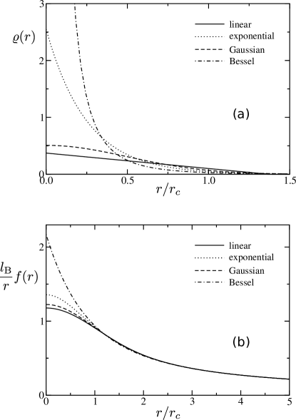
Figure 1: Charge density distributions (upper plot), and electrostatic interaction potentials (lower plot), for the four models in Table 1. Parameters are $\sigma=\lambda=0.5\,r_{c}$, $R=1.37\,r_{c}$ (i. e. matching $\langle r^{2}\rangle=0.75\,r_{c}^{2}$), and $l_{\mathrm{B}}=1.1\,r_{c}$. The overlap energy $\beta u_{0}$ is the contact value at $r\to 0$ in the lower plot.

An implication of $g=\tilde{\varrho}^{2}$ is that $g\geq 0$. In fact this provides a necessary and sufficient condition for the interaction potential to correspond to the interaction between (identical) charge clouds. For example the obvious truncation $\beta U=\beta u_{0}=l_{\mathrm{B}}/r_{c}$ for $r<r_{c}$ and $\beta U=l_{\mathrm{B}}/r$ for $r\geq r_{c}$ gives rise to $g(k)$ which oscillates in sign, and therefore does not correspond to the interaction between charge clouds (this does not necessarily preclude the use of this potential of course).

Expanding the Fourier representation of $\tilde{\varrho}(k)$ gives

$$\tilde{\varrho}(k)=1-{\textstyle{\frac{1}{6}}}k^{2}\langle r^{2}\rangle+O(k^{4})$$ (4)

where $\langle r^{2}\rangle={\int d^{3}{\mathbf{r}}\,r^{2}\varrho}$ is the second moment of the charge distribution. This expansion implies

$$g(k)=1-{\textstyle{\frac{1}{3}}}k^{2}\langle r^{2}\rangle+O(k^{4})\,.$$ (5)

This allows us to extract the second moment of the charge distribution from $g(k)$.

Now consider the overlap energy. We have

$$\begin{split}\frac{\beta u_{0}}{l_{\mathrm{B}}}=\lim_{r\to 0}\frac{f(r)}{r}&=\lim_{r\to 0}\frac{2}{\pi}\int_{0}^{\infty}\!\!dk\,\frac{\sin(kr)}{kr}g(k)\\ &{}\hskip 60.00009pt=({2}/{\pi}){\textstyle\int_{0}^{\infty}}\!dk\,g(k)\,.\end{split}$$ (6)

Again we have a result expressed in terms of the function $g(k)$. The final integral in Eq. (6) may be tractable even if the inverse sine transform is not.

Table 1 shows these properties calculated for the four smoothed charge models considered in this study.

III Screening properties

We now describe the screening properties of the four charge smoothing methods, in the context of the above mesoscale electrolyte model. The details are much the same as already presented for the Gaussian case Warren et al. (2013). We shall establish the conditions under which the screening length is real-valued and the extent to which it matches the expected Debye length in the physical system.

For the first step, the electrolyte model just described is structurally characterised by the pair distribution functions $g_{\mu\nu}(r)$. From these we define the total correlation functions $h_{\mu\nu}=g_{\mu\nu}-1$. At low densities and weak coupling (i. e. $l_{\mathrm{B}}$ small compared to the charge cloud size) the total correlation functions for the ionic species show a universal exponential decay at large distances, $h_{\pm\pm}\sim e^{-\kappa r}/r$ for $r\to\infty$, where $\kappa^{-1}$ is the (real-valued) screening length. On the other hand, at high densities and/or strong coupling, the functions $h_{\pm\pm}$ show damped oscillatory decay and the screening length becomes complex Janaček and Netz (2009). The two behaviours are separated by a sharp transition as a function of density and coupling strength, known as the Kirkwood line Kirkwood (1936).

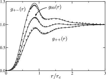
Figure 2: Comparison between HNC (solid lines) and simulation (circles, taken from Fig. 3 of Ref. Groot, 2003) for an electrolyte model with linear charge smoothing. Parameters are $|z_{\pm}|=1$, $l_{\mathrm{B}}=1.1\,r_{c}$, $R=1.6\,r_{c}$, $\rho r_{c}^{3}=3$, and $\rho_{z}r_{c}^{3}=0.2$; corresponding to a $0.6\,\mathrm{M}$ 1:1 aqueous electrolyte. The short range potential is $\phi(r)={\textstyle{\frac{1}{2}}}A(1-r/r_{c})^{2}$, with $A=25$.

Figure 3: Kirkwood lines in various representations (see text for details). The schematic insets indicate on which side of the Kirkwood line the total correlation functions $h_{\pm\pm}(r)$ exhibit pure exponential or damped oscillatory asymptotic decay.

III.1 Hypernetted chain (HNC) closure

We access the total correlation functions by solving the multicomponent hypernetted chain (HNC) integral equation closure for the fluid. This approximation has been extensively discussed in the existing literature Hansen and McDonald (2006); Vrbka et al. (2009), and is known to be quite accurate for these charged soft sphere models Coslovich et al. (2011b); Warren et al. (2013). For example, for linear screening, Fig. 2 shows the HNC pair distribution functions for the indicated state point compared to simulation results from Ref. Groot, 2003. The agreement is quite good. Other tests are reported in Ref. Warren et al., 2013, for the Gaussian charge model. Our HNC code uses potential splitting methods Springer et al. (1973); Ng (1974), and the only modification needed to the code used in Ref. Warren et al., 2013 is to swap in the generalised $g(k)$ functions in Table 1. In particular, it is not necessary to know the electrostatic pair potential in real space and $f(r)$ is not required.

The HNC Kirkwood lines for the four smoothed charge models are shown in Fig. 3, in three different representations. They are found by visually inspecting the asymptotic behaviour of the HNC total correlation functions. We use the iterative procedure outlined in Ref. Warren et al., 2013, stopping when the Kirkwood line has been located to around 1% accuracy in density. We have found that the Kirkwood lines and the screening behaviour in general is very insensitive (i. e. changes by at most by 1–2%) to the presence of the neutral solvent species and the short range repulsion. This is very helpful as it sharply reduces the complexity of the problem.

We note that the numerical solution method for HNC fails if the charge size becomes too small, typically less than 10% of $l_{\mathrm{B}}$. This loss of solution has also been observed by Coslovich, Hansen and Kahl for the URPM Coslovich et al. (2011b), and is almost certainly indicative of a mathematical property of HNC rather than a numerical problem.

The Kirkwood lines are plotted as functions of the ion density, using the native parameters (Fig. 3a), the second moment of the charge distribution (Fig. 3b), and the overlap energy (Fig. 3c). We see that the second representation brings the Kirkwood lines very close together. This implies Fig. 3b is a quasi-universal map which can be used as a guide for arbitrary smoothed charge models, provided that the second moment of the charge distribution is used as a length scale. Further confirmation of this role for $\langle r^{2}\rangle$ and a simple expression for the quasi-universal Kirkwood line is given in Section III.2. Examining the Kirkwood lines, it is obvious that the Bessel model is something of an outlier. In fact this is already apparent in Fig. 1 and Table 1, since unlike any of the other charge distributions, $\varrho(r)$ for the Bessel case diverges (as $1/r^{2}$) in the limit $r\to 0$.

The horizontal axis in the three plots in Fig. 3 is the ion density, drawn either as a dimensionless simulation variable $\rho_{z}r_{c}^{3}$ (upward pointing tick marks), or using physical units where $c_{s}$ is the ion concentration in Molar units (downward pointing tick marks). The two are related by a simple proportionality: given the choice $r_{c}=0.645\,\mathrm{nm}$ one has $\rho_{z}r_{c}^{3}\approx 0.32\,c_{s}/\,\mathrm{M}$.

At this point we should inject a note of common sense concerning the relevance of large values of $c_{s}$. In the physical system, the actual screening length is often taken to be the Debye length, given by the well known expression $\kappa_{\mathrm{D}}^{-1}=0.31\,\mathrm{nm}/\sqrt{c_{s}/\mathrm{M}}$, familiar from the field of colloid science Verwey and Overbeek (1948). The Debye length is a decreasing function of $c_{s}$, and $\kappa_{\mathrm{D}}^{-1}\lesssim r_{c}$ occurs for $c_{s}\gtrsim 0.23\,\mathrm{M}$. When the Debye length falls below the DPD particle size, it no longer makes sense to represent the behaviour by a sophisticated electrostatic model, since the charge interactions could equally be captured in the short range DPD potential. In any case, deviations from Debye-Hückel theory start to become significant for $c_{s}\gtrsim 0.1\,\mathrm{M}$ and specific ion effects become more and more important. These considerations mean that $c_{s}\approx 0.1$–$0.2\,\mathrm{M}$ is a natural upper limit for the attempt to match the screening properties of the mesoscale model to the physical system.

In terms of the maps in Fig. 3, this implies the screening behaviour is moot for such high values of $c_{s}$. Turning this around, we can use this to propose sensible limits for the parameters in the models. For example, reading from Fig. 3a, the requirement to remain on the ‘right’ side of the Kirkwood line (i. e. on the low density side where the model has a real-valued screening length) translates into natural upper bounds for $R$, $\lambda$, and $\sigma$, in units of $r_{c}$. Fig. 3b is most useful in this respect since (setting aside the Bessel model which we already acknowledge is an outlier) there is a quasi-universal Kirkwood line. Sensible screening behaviour for $c_{s}\lesssim 0.1$–$0.2\,\mathrm{M}$ corresponds to $\langle r^{2}\rangle\lesssim(1.3$–$2.5)\,r_{c}^{2}$. These bounds can be tightened still further by considering the behavior of the actual screening length—see Section IV.

Fig. 3c is less useful in this respect since the relevant Kirkwood lines are not as closely collapsed together as Fig. 3b. Nevertheless the map indicates one should ensure $\beta u_{0}\gtrsim 0.6$–0.9. It is worth remarking that heuristic considerations led Groot to propose $\beta u_{0}\approx 1$ as the criterion for choosing $R$ in the linear smoothing model Groot (2003), and this was later taken over to the exponential smoothing case by González-Melchor et al. González-Melchor et al. (2006). This is in accord with the present analysis. Note however one should not increase $\beta u_{0}$ too much (equivalent to shrinking the charge cloud size), since that would lead towards the aforementioned low temperature artefacts (clustering, phase separation, et c.).

III.2 Random phase approximation (RPA)

Another well-trodden approach, also known to be quite accurate for these charged soft sphere models, is the random phase approximation (RPA). In this case an analytic solution for the Fourier-transformed total correlation functions can be obtained. The solution method is described in Ref. Warren et al., 2013. The general result is

$$\tilde{h}_{\mu\nu}=-\frac{4\pi l_{\mathrm{B}}z_{\mu}z_{\nu}g(k)}{k^{2}+\kappa_{\mathrm{D}}^{2}g(k)}-\frac{\tilde{\phi}}{1+\rho\tilde{\phi}}\,.$$ (7)

Again we see the relevance of the ‘glue’ function, $g(k)$, which together with $\tilde{\phi}(k)$ contains all the model-dependent features.

In Eq. (7)

$$\kappa_{\mathrm{D}}^{2}=4\pi l_{\mathrm{B}}\,{\textstyle\sum_{\mu}}z_{\mu}^{2}\,\rho_{\mu}$$ (8)

is the square of the Debye wavevector, so that $\kappa_{\mathrm{D}}^{-1}$ is the already-introduced Debye length. For a 1:1 electrolyte, $\kappa_{\mathrm{D}}^{2}=4\pi l_{\mathrm{B}}\rho_{z}$ (in the physical system, this gives rise to the expression used earlier from the colloid literature).

The asymptotic behaviour of $h_{\pm\pm}(r)$ is determined by the positions of the poles of $\tilde{h}_{\pm\pm}(k)$, regarded as analytic functions in the complex $k$-plane Evans et al. (1994); Hopkins et al. (2006); Nikoubashman et al. (2012). The functions share a common set of poles. There are two typical scenarios. If the nearest pole to the real axis is purely imaginary, the asymptotic behaviour of $h_{\pm\pm}(r)$ is purely exponential and there is a real-valued screening length set by the distance of the pole from the real axis. Alternatively, if the nearest poles to the real axis are complex, the asymptotic behaviour of $h_{\pm\pm}(r)$ is damped oscillatory and the screening length is complex. The Kirkwood line is determined by the crossover between the two scenarios.

In the case of the RPA, there are two sets of poles arising from the two contributions to $\tilde{h}_{\pm\pm}$ in Eq. (7). Of these, the poles from the second term (arising from the short range repulsion) are usually too distant from the real axis to be relevant; therefore we focus attention on the first term (arising from the electrostatics). The poles in this term correspond to the zeros of

$$k^{2}+\kappa_{\mathrm{D}}^{2}\,g(k)=0\,.$$ (9)

Since $\kappa_{\mathrm{D}}\to 0$ at low densities, this equation can be solved iteratively, using Eq. (5) for the expansion of $g(k)$ about $k=0$. We find that the relevant zero is purely imaginary and the corresponding screening length is given by

$$\kappa^{-1}=\kappa_{\mathrm{D}}^{-1}[1-{\textstyle{\frac{1}{6}}}\langle r^{2}\rangle\kappa_{\mathrm{D}}^{2}+O(\kappa_{\mathrm{D}}^{4})]\,.$$ (10)

Thus we see that, as the ion density decreases, the screening length approaches the Debye length, from below, by an amount controlled by $\langle r^{2}\rangle$. This is lends weight to the argument that $\langle r^{2}\rangle$ is a good choice for matching between smoothing methods, when it comes to predicting the screening properties.

For the Gaussian and Bessel cases, the zeros of Eq. (9) can be obtained analytically Nikoubashman et al. (2012); Warren and Masters (2013); Warren et al. (2013). The corresponding Kirkwood lines lie at $\kappa_{\mathrm{D}}\sigma=e^{-1/2}$ for the Gaussian case, and $\kappa_{\mathrm{D}}\sigma={\textstyle{\frac{1}{2}}}$ for the Bessel case. In fact for $\sigma/r_{c}\gtrsim 0.3$ these are practically indistinguishable from the HNC result (see also Fig. 5 in Ref. Warren et al., 2013). This means that the quasi-universal Kirkwood line in Fig. 3b is given by (Gaussian case)

$$\frac{\langle r^{2}\rangle}{r_{c}^{2}}=\frac{3}{4\pi el_{\mathrm{B}}\rho_{z}r_{c}^{2}}\approx\frac{0.081}{\rho_{z}r_{c}^{3}}\approx\frac{0.253\,\mathrm{M}}{c_{s}}\,.$$ (11)

Generally, for the RPA, we can infer from Eq. (9) that the Kirkwood line corresponds to some particular value of $\kappa_{\mathrm{D}}$, measured in units of the size of the charge clouds. This is because the latter length scale is the only one available to non-dimensionalise the argument of $g(k)$ (for examples, see Table 1). Since $\kappa_{\mathrm{D}}\propto 1/\sqrt{\rho_{z}}$, and we have seen that the RPA is quite accurate, this observation explains the slopes of the Kirkwood lines in Fig. 3.

Another point to note from Eq. (7) is that if the screening properties are governed solely by the first term, the second term can be neglected. This implies that in the RPA the screening properties are completely insensitive to the presence of the neutral solvent species and short range repulsions. This explains the similar observation made for the HNC.

IV Final recommendations

The charge cloud size arising from the smoothing operation is not supposed to have a physical significance and can be chosen to maximise computational efficiency. For example, a large amount of smoothing means that one can use a coarse mesh spacing in a P³M method, or fewer terms in an Ewald sum in other methods. But as we have seen this is in direct competition with the desire to avoid unwanted artefacts, such as damped oscillatory behaviour in the total correlation functions which arises when one is on the ‘wrong’ side of the Kirkwood line. Clearly then, the incentive is to push the charge cloud size towards the upper bounds indicated in the discussion in Section III.1.

Specific requirements for the screening behaviour can then be used to sharpen these bounds. Thus in Ref. Warren et al., 2013 we suggested $\sigma=0.5\,r_{c}$ for the Gaussian case, since this means that there is a real-valued screening length, within 10% of the Debye length, for 1:1 electrolyte solutions with $c_{s}\lesssim 0.15\,\mathrm{M}$. We can translate this into suggested parameter values for other smoothing models by matching the second moment of the charge distribution, namely $\langle r^{2}\rangle=0.75\,r_{c}^{2}$. Using the final column in Table 1, this corresponds to the choices

$$\sigma=\lambda=0.5\,r_{c}\,,\quad\text{or}\quad R\approx 1.37\,r_{c}\,.$$ (12)

When we compute the screening length for a $c_{s}=0.15\,\mathrm{M}$ 1:1 electrolyte with these parameters, we find that all the methods give a value within 1% of $\kappa^{-1}\approx 1.11\,r_{c}\approx 0.72\,\mathrm{nm}$. This can be compared to $\kappa_{\mathrm{D}}^{-1}\approx 0.31\,\mathrm{nm}/\sqrt{c_{s}}\approx 0.80\,\mathrm{nm}$. Thus the parameters in Eq. (12) are not only self consistent, but lead to a screening length within 10% of the Debye length Cno . Furthermore, the agreement will improve as $c_{s}$ decreases. Eq. (12) thus represents our recommended choice of parameters for the available mesoscale electrolyte models used in DPD. For comparison, Groot recommended $R=1.6\,r_{c}$ for the linear smoothing model, and González-Melchor et al. recommended $\lambda=1.08\,r_{c}$ for the exponential smoothing model. Thus our own recommendations are somewhat more stringent but come with guaranteed behaviour in terms of the screening properties.

Although our analysis has been confined to 1:1 aqueous electrolytes, it is not necessarily that restrictive since the methods used here can in principle be transferred to other situations, such as concentrated or multivalent electrolytes, and non-aqueous solvents. An ultimate goal is to incorporate specific ion effects into the models, such as the Hofmeister series Collins and Washabaugh (1985). Mindful of this, and the utility of a fast, accurate, multicomponent integral equation code in general, we have made available the FORTRAN 90 source code used in these calculations as fully documented open source software OZn .

We thank Lucian Anton and Andrew Masters for their generous advice and guidance. In particular we acknowledge that the computer code used here was based on a HNC code originally developed by Lucian. We additionally thank Andrew for hosting visits of one of us (AV) and providing a stimulating environment in which the work was done. We would also like to acknowledge the contribution of Ming Li, who noted the structure of the RPA solution for ions and neutral spheres in a related context. AV acknowledges partial support for trips to the UK from grant RFBR #13-03-01111.

References

- Frenkel and Smit (2002) D. Frenkel and B. Smit, Understanding molecular simulation (Academic Press, San Diego, 2002).
- Noro et al. (2003) M. G. Noro, F. Meneghini, and P. B. Warren, ACS Symp. series 861, 242 (2003).
- Groot (2003) R. D. Groot, J. Chem. Phys. 118, 11265 (2003).
- Fisher and Ruelle (1966) M. E. Fisher and D. Ruelle, J. Math. Phys. 7, 260 (1966).
- González-Melchor et al. (2006) M. González-Melchor, E. Mayoral, M. E. Velázquez, and J. Alejandre, J. Chem. Phys. 125, 224107 (2006).
- Warren et al. (2013) P. B. Warren, A. Vlasov, L. Anton, and A. J. Masters, J. Chem. Phys. 138, 204907 (2013).
- Coslovich et al. (2011a) D. Coslovich, J.-P. Hansen, and G. Kahl, Soft Matter 7, 1690 (2011a).
- Coslovich et al. (2011b) D. Coslovich, J.-P. Hansen, and G. Kahl, J. Chem. Phys. 134, 244514 (2011b).
- Nikoubashman et al. (2012) A. Nikoubashman, J.-P. Hansen, and G. Kahl, J. Chem. Phys. 137, 094905 (2012).
- Warren and Masters (2013) P. B. Warren and A. J. Masters, J. Chem. Phys. 138, 074901 (2013).
- Hansen and McDonald (2006) J.-P. Hansen and I. R. McDonald, Theory of simple liquids (Academic Press, Amsterdam, 2006).
- Levin (2002) Y. Levin, Rep. Prog. Phys. 65, 1577 (2002).
- Janaček and Netz (2009) J. Janaček and R. R. Netz, J. Chem. Phys. 130, 074502 (2009).
- Kirkwood (1936) J. G. Kirkwood, Chem. Rev. 19, 275 (1936).
- Vrbka et al. (2009) L. Vrbka, M. Lund, I. Kalcher, J. Dzubiella, R. R. Netz, and W. Kunz, J. Chem. Phys. 131, 154109 (2009).
- Springer et al. (1973) J. F. Springer, M. A. Pokrant, and F. A. Stevens Jr., J. Chem. Phys. 58, 4863 (1973).
- Ng (1974) K.-C. Ng, J. Chem. Phys. 61, 2680 (1974).
- Verwey and Overbeek (1948) E. J. W. Verwey and J. Th. G. Overbeek, Theory of the stability of lyophobic colloids (Elsevier, Amsterdam, 1948).
- Evans et al. (1994) R. Evans, R. J. F. Leote de Carvalho, J. R. Henderson, and D. C. Hoyle, J. Chem. Phys. 100, 591 (1994).
- Hopkins et al. (2006) P. Hopkins, A. J. Archer, and R. Evans, J. Chem. Phys. 124, 054503 (2006).
- (21) Since , most of this difference is explained by the leading correction in Eq. (10).
- Collins and Washabaugh (1985) K. D. Collins and M. W. Washabaugh, Quart. Rev. Biophys. 18, 323 (1985).
- (23) See http://sunlightdpd.sourceforge.net/ to download the source code.