On singular value distribution of large-dimensional autocovariance matrices

Abstract

Let $(\varepsilon_{j})_{j\geq 0}$ be a sequence of independent $p-$dimensional random vectors and $\tau\geq 1$ a given integer. From a sample $\varepsilon_{1},\cdots,\varepsilon_{T+\tau-1},\varepsilon_{T+\tau}$ of the sequence, the so-called lag$-\tau$ auto-covariance matrix is $C_{\tau}=T^{-1}\sum_{j=1}^{T}\varepsilon_{\tau+j}\varepsilon_{j}^{t}$. When the dimension $p$ is large compared to the sample size $T$, this paper establishes the limit of the singular value distribution of $C_{\tau}$ assuming that $p$ and $T$ grow to infinity proportionally and the sequence satisfies a Lindeberg condition. Compared to existing asymptotic results on sample covariance matrices developed in random matrix theory, the case of an auto-covariance matrix is much more involved due to the fact that the summands are dependent and the matrix $C_{\tau}$ is not symmetric. Several new techniques are introduced for the derivation of the main theorem.

, and t1Corresponding author.

1 Introduction

Let $\varepsilon_{1},\ldots,\varepsilon_{T+\tau}$ be a sample from a stationary process with values in $\mathbb{R}^{p}$. The $p\times p$ matrix

$$C_{\tau}:=\frac{1}{T}\sum_{j=1}^{T}\varepsilon_{\tau+j}\varepsilon_{j}^{t},$$ (1.1)

is the so-called lag$-\tau$ sample auto-covariance matrix of the process (here $u^{t}$ denotes the transpose of a vector or matrix $u$). In a classical low-dimensional situation where the dimension $p$ is assumed much smaller than the sample size $T$, $C_{\tau}$ is very close to $\mathop{\mathbb{E}}C_{\tau}=\mathop{\mathbb{E}}\varepsilon_{1+\tau}\varepsilon_{1}^{t}$ so that its asymptotic behavior when $T\to\infty$ (so $p$ is considered as fixed) is well known. In the high-dimensional context where typically the dimension $p$ is of same order as $T$, $C_{\tau}$ will not converge to $\mathop{\mathbb{E}}C_{\tau}$ and its asymptotic properties have not been well investigated. In this paper, we study the empirical spectral distribution (ESD) of $C_{\tau}$, namely, the distribution generated by its $p$ singular values. The main result of the paper is the establishment of the limit of this ESD when $(\varepsilon_{j})$ is an independent sequence with elements having a finite fourth moments while $p$ and $T$ grow to infinity proportionally.

In order to understand the importance of limiting spectral distribution (LSD) of singular values of the auto-covariance matrix $C_{\tau}$, we describe a statistical problem where these distributions are of central interest. In a recent stimulating paper, Lam and Yao [6] considers the following dynamic factor model

$${x}_{i}=\Lambda{f}_{i}+\varepsilon_{i}+\mu,$$ (1.2)

where $\{{x}_{i};~{}0\leq i\leq T\}$ is an observed $p$-dimensional sequence, $\{f_{i}\}$ a sequence of $m$-dimensional “latent factor” ($m\ll p$) uncorrelated with the error process $\{\varepsilon_{i}\}$ and $\mu\in\mathbb{R}^{p}$ is the general mean. A particularly important question here is the determination of the number $m$ of factors. For any stationary process $\{w_{i}\}$, let ${\Sigma}_{w}=\mathop{\text{cov}}({w}_{i},{w}_{i-1})$ be its (population) lag-$1$ auto-covariance matrix, we have

$${\Sigma}_{x}=\Lambda{\Sigma}_{f}\Lambda^{t}.$$

It turns out that ${\Sigma}_{x}$ has exactly $m$ non-null singular values so that based on a sample ${x}_{0},{x}_{1},\ldots,{x}_{T}$ it seems natural to infer $m$ from the singular values of the sample lag-1 auto-covariance matrix

$$\Gamma_{x} = \frac{1}{T}\sum_{j=1}^{T}(\Lambda{f}_{j}+\varepsilon_{j})(\Lambda{f}_{j-1}+\varepsilon_{j-1})^{t}$$

$$= \Lambda\left(\frac{1}{T}\sum_{j=1}^{T}{f}_{j}{f}^{t}_{j-1}\right)\Lambda^{t}+\Lambda\left(\frac{1}{T}\sum_{j=1}^{T}{f}_{j}\varepsilon^{t}_{j-1}\right)+\left(\frac{1}{T}\sum_{j=1}^{T}\varepsilon_{j}{f}^{t}_{j-1}\right)\Lambda^{t}+C_{1}~{}.$$

Because $\Lambda$ has rank $m$, the first three terms all have rank bounded by $m$ and $\Gamma_{x}$ appears as a finite-rank perturbation of the lag-1 auto-covariance matrix $C_{1}$ which in general has rank $p\gg m$. Therefore, understanding the properties of the singular values of $C_{1}$ will be of primary importance for the understanding of the $m$ largest singular values of the matrix of $\Gamma_{x}$ which are, as said above, fundamental for the determination of the number of factors $m$. Notice however that this statistical problem is given here to describe a potential application of the theory established in this paper, but this theory on singular value distribution is general and can be applied to fields other than statistics.

If we take $\tau=0$ in (1.1), the matrix $S=\frac{1}{T}\sum_{j=1}^{T}\varepsilon_{j}\varepsilon_{j}^{t}$ is the sample covariance matrix from the observations. The theory for eigenvalue distributions of $S$ has been extensively studied in the random matrix literature dating back to the seminal paper [7]. In this paper, the famous Mar$\check{c}$enko-Pastur law as limit of eigenvalue distributions has been found for a wide class of sample covariance matrices. Further development includes the almost sure convergence of these distributions ([9]) and conditions for convergence of the largest and the smallest eigenvalues, see [4]. Meanwhile book-length analysis of sample covariance matrices can be found in [3], [1], [8]. The situation of an auto-covariance matrix $C_{\tau}$ is completely different. To author’s best knowledge, none of the existing literature in random matrix theory treats the sample auto-covariance matrix and the limit for its eigenvalue distribution found in this paper is new.

There are basically two major differences between $C_{\tau}$ and $S$. First, while $S$ is a non-negative symmetric random matrix, $C_{\tau}$ is even not symmetric and we must rely on singular value distributions which are in general much more involved than eigenvalue distributions. Secondly, because of the positive lag $\tau$, the summands in $C_{\tau}$ are no more independent as it is the case for the sample covariance matrix $S$. This again makes the analysis of $C_{\tau}$ more difficult. As a consequence of these major differences, several new techniques are introduced in the paper in order to complete the proofs, although the general strategy is common in the random matrix theory (see Bai and Silverstein [3], Pastur and Shcherbina [8]). For example, the characterization of the Stieltjes transform of the limiting distribution is obtained via a system of equations due to the time delay $\tau$ where for the case of sample covariance matrix, the characterization is given by a single equation([7], [9]).

The rest of the paper is organized as follows. The main theorem of the paper is introduced in Section 2. Section 3 details the proof of the main theorem when time lag $\tau=1$. Section  4 generalizes the proof from time lag $\tau=1$ to any given positive number. Meanwhile, in contrast to other aspects discussed above, the preliminary steps of truncation, centralization and standardization of the matrix entries are similar to the case of a sample covariance matrix. They are given in Appendix A. To ease the reading of the proof, technical lemmas are grouped in Section 5.

2 Main Results

In this paper, we intend to derive the limiting singular value distribution of the lag$-\tau$ auto-covariance matrix defined in (1.1). It will be done in two steps. We derive the main result first for the lag-1$(\tau=1)$ sample auto-covariance matrix $C_{1}=\frac{1}{T}\sum_{t=1}^{T}\varepsilon_{j}\varepsilon_{j-1}^{t}$. It turns out that the general case $\tau\geq 1$ is essentially the same and the extension is easily obtained. The details of the extension are given in Section 4.

Therefore, we consider the lag-1 sample auto-covariance matrix $C_{1}=\frac{1}{T}\sum_{j=1}^{T}\varepsilon_{j}\varepsilon_{j-1}^{t}$. By definition, it is equivalent to study the limiting spectral distribution(LSD) of the matrix

$$A=C_{1}C_{1}^{t}=\frac{1}{T^{2}}(\sum_{j=1}^{T}\varepsilon_{j}\varepsilon^{t}_{j-1})(\sum_{j=1}^{T}\varepsilon_{j-1}\varepsilon^{t}_{j}).$$

Alternatively,

$$A=\frac{1}{T^{2}}XY^{t}YX^{t},$$

where $X=\left(\varepsilon_{1},\cdots,\varepsilon_{T}\right)_{p\times T}$, $Y=\left(\varepsilon_{0},\cdots,\varepsilon_{T-1}\right)_{p\times T}$. Here we define a modified version of the A matrix,

$$B=\frac{1}{T^{2}}Y^{t}YX^{t}X=\sum_{j=1}^{p}s_{j}s_{j}^{t}\sum_{j=1}^{p}r_{j}r_{j}^{t},$$

where $s_{j}=\frac{1}{\sqrt{T}}\left(\varepsilon_{j0},\varepsilon_{j1},\cdots,\varepsilon_{j,T-1}\right)^{t}$ is the j-th row of $Y$, and $r_{j}=\frac{1}{\sqrt{T}}\left(\varepsilon_{j1},\varepsilon_{j2},\cdots,\varepsilon_{j,T}\right)^{t}$ the j-th row of $X$. As $A$ and $B$ have same nonzero eigenvalues, the LSD of $A$ can be derived from the LSD of $B$.

The main result of the paper is

Theorem 2.1.

Let the following assumptions hold:

• $\varepsilon_{i}=\left(\varepsilon_{1i},\cdots\varepsilon_{pi}\right)^{t},i=0,1,2,\cdots,T$ are independent p-dimensional real-valued random vectors with independent entries satisfying condition:

  $$\mathbb{E}(\varepsilon_{it})=0,~{}\mathbb{E}(\varepsilon^{2}_{it})=1,~{}\sup_{1\leq i\leq p,0\leq t\leq T}\mathbb{E}\left(|\varepsilon_{it}|^{4}\right)<M,$$

  for some constant $M$ and for any $\eta>0$,

  $$\frac{1}{\eta^{4}pT}\sum_{i=1}^{p}\sum_{t=0}^{T}\mathbb{E}\left(|\varepsilon_{it}|^{4}I_{(|\varepsilon_{it}|\geq\eta T^{1/4})}\right)=o\left(1\right);$$

• As $p\rightarrow\infty$, the sample size $T=T(p)\rightarrow\infty$ and $p/T\rightarrow c>0$.

Then,

• as $p,T\rightarrow\infty$, almost surely, the empirical spectral distribution $F^{B}$ of $B$, converges to a non-random probability distribution $\b{F}$ whose Stieltjes transform $x=x(\alpha)$, $\alpha\in\mathbb{C}\setminus\mathbb{R}$, satisfies the equation

  $$\alpha^{2}x^{3}-2\alpha\left(c-1\right)x^{2}+\left(c-1\right)^{2}x-\alpha x-1=0.$$ (2.1)

• Moreover, for $\alpha\in\mathbb{C}^{+}=\{z:\mathfrak{Im}z>0\}$, equation (2.1) admits an unique solution $\alpha\mapsto x(\alpha)$ with positive imaginary part and the density function of the LSD $\b{F}$ is:

  $\displaystyle f(u)$ $\displaystyle=\frac{1}{\pi u}\left\{-u-\frac{5(c-1)^{2}}{3}+\frac{2^{4/3}(3u+(c-1)^{2})(c-1)}{3d(u)^{1/3}}+\frac{2^{2/3}(c-1)d(u)^{1/3}}{3}\right.$ $\displaystyle\quad+\left.\frac{1}{48}\left[-8(c-1)+\frac{2\times 2^{1/3}(3u+(c-1)^{2})}{d(u)^{1/3}}+2^{2/3}d(u)^{1/3}\right]^{2}\right\}^{1/2},$

  where $d(u)=-2(c-1)^{3}+9(1+2c)u+3\sqrt{3}\sqrt{u(-4u^{2}+(-1+4c(5+2c))u-4c(c-1)^{3})}$.

  Moreover, the support of f(u) is $(0,b]$ for $0<c\leq 1$, and $[a,b]$ for $c>1$, where

  $$a=\frac{1}{8}(-1+20c+8c^{2}-(1+8c)^{3/2}),\quad b=\frac{1}{8}(-1+20c+8c^{2}+(1+8c)^{3/2}).$$

It’s easy to check that when $c<1$, the LSD of $B$ has a point mass $1-c$ at the origin since $\mathrm{rank}(B)=p<T$ for large $p$ and $T$, and at the same time we have

$$\left\{\begin{array}[]{l}\displaystyle\int_{0}^{b}f(u)du=c,\quad 0<c<1,\\[4.2679pt] \displaystyle\int_{a}^{b}f(u)du=1,\quad c\geq 1.\end{array}\right.$$

Since the matrix $A$ we are interested in has the same non-zero eigenvalues with $B$, the following proposition holds.

Proposition 2.1.

Under the conditions of Theorem 2.1, the ESD of $A$ converges a.s. to a non-random limit distribution

$$F=\frac{1}{c}\b{F}+(1-\frac{1}{c})\delta_{0},$$

whose Stieltjes transform $y=y(\alpha)$, $\alpha\in\mathbb{C}\setminus\mathbb{R}$, satisfies the equation

$$\alpha^{2}c^{2}y^{3}+\alpha c(c-1)y^{2}-\alpha y-1=0.$$

In particular, $F$ has the density function

$$\left\{\begin{array}[]{l}\displaystyle\frac{1}{c}f(u),~{}u\in(0,b],\mbox{ for }0<c<1,\\[4.2679pt] \displaystyle\frac{1}{c}f(u),~{}u\in[a,b],\mbox{ for }c\geq 1.\end{array}\right.$$

where in the later case $c\geq 1$, $F$ has an additional mass $(1-\frac{1}{c})$ at the origin.

The following details the density function of LSD of $A$ for different values of c.

• When $c=1$, the support is $0\leq u\leq\frac{27}{4}$ and the density function is

  $$\frac{1}{c}f(u)=\frac{1}{\pi u}\left[-u+3\left(\frac{u}{2^{2/3}d(u)^{1/3}}+\frac{d(u)^{1/3}}{6\times 2^{1/3}}\right)^{2}\right]^{1/2},$$

  where $d(u)=27u+3\sqrt{3}\times\sqrt{u(-4u^{2}+27u)}$. It’s easy to see that as $u\rightarrow 0_{+}$, $f(u)\rightarrow\infty$.

• If $c<1$, it can be seen from the explicit form of $f(u)$ that when $u\rightarrow 0_{+}$, $\frac{1}{c}f(u)\rightarrow\infty$ because the $u$ in the denominator of the density function cannot be completely canceled out.

• If $c>1$, the shape of the density function turns out to be a little different from the case $c\leq 1$. Nevertheless it’s quite intuitive because the lower bound of the support is positive and the density function is bounded.

The density functions of LSD of A for $c=0.5,1,2,3$ are displayed on Figure 1.

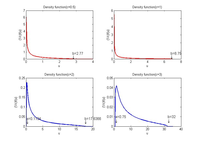
Figure 1: Density plots of the LSD of B.Top to bottom and left to right: c=0.5,1,2 and 3, respectively

3 Proofs

3.1 Proof of Theorem 2.1

The proof of the theorem follows the general strategy based on the Stieltjes transform as presented in Silverstein [9], Bai and Silverstein [3] and Pastur and Shcherbina [8]. However, the random matrix B here is no more a covariance matrix as considered in these references. Almost all the steps of the proof need new arguments and ideas compared to the case of sample covariance matrices considered so far in the literature. Following this method, the first step is to truncate the entries $\{\varepsilon_{jt}\}$ at a convenient rate using Assumption (a). After truncation and the follow-up steps of centralization and standardization, we may assume that

$$|\varepsilon_{ij}|\leq\eta T^{1/4},\quad\mathbb{E}\left(\varepsilon_{ij}\right)=0,\quad Var\left(\varepsilon_{ij}\right)=1,\quad\sup_{1\leq i\leq p,0\leq j\leq T}\mathbb{E}\left(|\varepsilon_{ij}|^{4}\right)<M.$$

The details of these technical steps are given in Appendix A.

By the rank inequality(Theorem A.44 of [3]), it is enough to consider

$$B=\sum_{j=1}^{p}s_{j}s_{j}^{t}\sum_{j=1}^{p}r_{j}r_{j}^{t}=P_{1}\tilde{C}P_{1}^{t}\tilde{C},$$

where

$$s_{j}=P_{1}r_{j}=\frac{1}{\sqrt{T}}(0,\varepsilon_{j1},\cdots,\varepsilon_{j,T-1})^{t},\quad C=\sum_{j=1}^{p}s_{j}s_{j}^{t},\quad\tilde{C}=\sum_{j=1}^{p}r_{j}r_{j}^{t},\quad P_{1}=\left(\begin{array}[]{cc}\textbf{0}&0\\ \textbf{I}_{T-1}&\textbf{0}\end{array}\right).$$

At this stage, the important observation is that here we have replaced $s_{j}=\frac{1}{\sqrt{T}}(\varepsilon_{j0},\varepsilon_{j1},\cdots,\varepsilon_{j,T-1})^{t}$ by $\tilde{s}_{j}=\frac{1}{\sqrt{T}}(0,\varepsilon_{j1},\cdots,\varepsilon_{j,T-1})^{t}$ without altering the LSD of B since when $T\rightarrow\infty$, the effect of this substitution will vanish. For the sake of convenience, we still use $s_{j}$ to denote $\tilde{s}_{j}$.

For $\alpha\in\mathbb{C}\setminus\mathbb{R}$, define

$$B\left(\alpha\right)=\sum_{j=1}^{p}s_{j}s_{j}^{t}\sum_{j=1}^{p}r_{j}r_{j}^{t}-\alpha I_{T}.$$

Let

$$x_{0}=\frac{1}{T}tr(B^{-1}(\alpha)),\quad y_{0}=\frac{1}{T}tr(\tilde{C}B^{-1}(\alpha)),\quad z_{0}=\frac{1}{T}tr(B^{-1}(\alpha)C).$$

The method consists in finding a system of two asymptotic equations satisfied by $x_{0}$ and $y_{0}$. Solving the system yields an asymptotic equivalent for $x_{0}$ and finally leads to the equation (2.1) satisfied by the limit of $x_{0}$. Nonetheless, $x_{0}$ is the Stieltjes transform of the matrix B which can be recovered from the inversion formula.

Let

$$B_{j}\left(\alpha\right)=\sum_{k\neq j}s_{k}s_{k}^{t}\sum_{i\neq j}r_{i}r_{i}^{t}-\alpha I_{T},\quad C_{j}=C-s_{j}s_{j}^{t},\quad\tilde{C}_{j}=\tilde{C}-r_{j}r_{j}^{t},\quad 1\leq j\leq p,$$

then

$$B\left(\alpha\right) =B_{j}\left(\alpha\right)+\sum_{i\neq j}s_{j}s_{j}^{t}r_{i}r_{i}^{t}+\sum_{k\neq j}s_{k}s_{k}^{t}r_{j}r_{j}^{t}+s_{j}s_{j}^{t}r_{j}r_{j}^{t}$$

$$=B_{j}\left(\alpha\right)+s_{j}s_{j}^{t}\tilde{C}_{j}+C_{j}r_{j}r_{j}^{t}+s_{j}s_{j}^{t}r_{j}r_{j}^{t}.$$

We have

$$I_{T}=B(\alpha)B^{-1}(\alpha)=\left(\sum_{j=1}^{p}s_{j}s_{j}^{t}\right)\left(\sum_{j=1}^{p}r_{j}r_{j}^{t}\right)B^{-1}\left(\alpha\right)-\alpha B^{-1}\left(\alpha\right).$$

Taking trace and dividing both sides by $T$, we get

$$1=\frac{1}{T}\sum_{j=1}^{p}s_{j}^{t}\tilde{C}B^{-1}\left(\alpha\right)s_{j}-\alpha\frac{1}{T}tr\left(B^{-1}\left(\alpha\right)\right).$$ (3.1)

Note that $x_{0}=\frac{1}{T}tr(B^{-1}(\alpha))$ is the Stieltjes transform of the ESD of the matrix B, and its limit will be found by letting $p,T\rightarrow\infty$ on both sides of the equation.

Consider $s_{j}^{t}\tilde{C}B^{-1}\left(\alpha\right)s_{j}$, using the identities

$$\left(B+\sum_{j=1}^{m}ab_{j}^{t}\right)^{-1}a=\frac{B^{-1}a}{1+\sum_{j=1}^{m}b_{j}^{t}B^{-1}a},$$

and

$$B^{-1}-D^{-1}=B^{-1}\left(D-B\right)D^{-1},$$

we have

$$s_{j}^{t}\tilde{C}B^{-1}\left(\alpha\right)s_{j} =\frac{s_{j}^{t}\tilde{C}\left(B_{j}\left(\alpha\right)+C_{j}r_{j}r_{j}^{t}\right)^{-1}s_{j}}{1+s_{j}^{t}\tilde{C}\left(B_{j}\left(\alpha\right)+C_{j}r_{j}r_{j}^{t}\right)^{-1}s_{j}}$$

$$=1-\frac{1}{1+s_{j}^{t}\tilde{C}_{j}\left(B_{j}\left(\alpha\right)+C_{j}r_{j}r_{j}^{t}\right)^{-1}s_{j}+s_{j}^{t}r_{j}r_{j}^{t}\left(B_{j}\left(\alpha\right)+C_{j}r_{j}r_{j}^{t}\right)^{-1}s_{j}}$$

$$:=1-\frac{1}{1+L_{1}+L_{2}},$$

where $L_{1}$ and $L_{2}$ are explicitly defined.

For $L_{1}$, by Lemma 5.1, or equivalently by Lemma 2.7 of [2], we have

$$L_{1} = s_{j}^{t}\tilde{C}_{j}\left(B_{j}\left(\alpha\right)+C_{j}r_{j}r_{j}^{t}\right)^{-1}s_{j}$$

$$= s_{j}^{t}\tilde{C}_{j}B_{j}^{-1}\left(\alpha\right)s_{j}-s_{j}^{t}\tilde{C}_{j}B_{j}\left(\alpha\right)^{-1}C_{j}r_{j}r_{j}^{t}\left(B_{j}\left(\alpha\right)+C_{j}r_{j}r_{j}^{t}\right)^{-1}s_{j}$$

$$= s_{j}^{t}\tilde{C}_{j}B_{j}^{-1}\left(\alpha\right)s_{j}-\frac{s_{j}^{t}\tilde{C}_{j}B_{j}^{-1}\left(\alpha\right)C_{j}r_{j}r_{j}^{t}B_{j}\left(\alpha\right)^{-1}s_{j}}{1+r_{j}^{t}B_{j}^{-1}\left(\alpha\right)C_{j}r_{j}}$$

$$= \frac{1}{T}tr\left(\tilde{C}_{j}B_{j}^{-1}\left(\alpha\right)\right)-\frac{\frac{1}{T}tr\left(\tilde{C}_{j}B_{j}^{-1}\left(\alpha\right)C_{j}P_{1}^{t}\right)\cdot\frac{1}{T}tr\left(B_{j}^{-1}\left(\alpha\right)P_{1}\right)}{1+\frac{1}{T}tr\left(B_{j}\left(\alpha\right)^{-1}C_{j}\right)}+o_{a.s.}(1).$$

For $L_{2}$, we have

$$L_{2} =s_{j}^{t}r_{j}r_{j}^{t}\left(B_{j}\left(\alpha\right)+C_{j}r_{j}r_{j}^{t}\right)^{-1}s_{j}=s_{j}^{t}r_{j}r_{j}^{t}B_{j}^{-1}\left(\alpha\right)s_{j}-\frac{s_{j}^{t}r_{j}r_{j}^{t}B_{j}^{-1}\left(\alpha\right)C_{j}r_{j}r_{j}^{t}B^{-1}_{j}(\alpha)s_{j}}{1+r_{j}^{t}B_{j}^{-1}\left(\alpha\right)C_{j}r_{j}}$$

$$=\left(s_{j}^{t}P_{1}^{t}s_{j}\right)\cdot\frac{1}{T}tr\left(B_{j}^{-1}\left(\alpha\right)P_{1}\right)-\frac{\left(s_{j}^{t}P_{1}^{t}s_{j}\right)\cdot\frac{1}{T}tr\left(B_{j}^{-1}(\alpha)C_{j}\right)\cdot\frac{1}{T}tr\left(B_{j}^{-1}\left(\alpha\right)P_{1}\right)}{1+\frac{1}{T}tr\left(B_{j}^{-1}\left(\alpha\right)C_{j}\right)}+o_{a.s.}(1)=o_{a.s.}(1).$$

Therefore, by equation $\eqref{eq:1}$, we have

$$~{}1+\alpha\frac{1}{T}tr(B^{-1}(\alpha))=o_{a.s.}(1)+$$ (3.2)

$$\frac{p}{T}\left(1-\dfrac{1+\dfrac{1}{T}tr(B^{-1}(\alpha)C)}{\left(1+\dfrac{1}{T}tr\left(B^{-1}(\alpha)C\right)\right)\left(1+\dfrac{1}{T}tr(\tilde{C}B^{-1}(\alpha))\right)-\dfrac{1}{T}tr\left(\tilde{C}B^{-1}\left(\alpha\right)CP_{1}^{t}\right)\cdot\dfrac{1}{T}tr\left(B^{-1}\left(\alpha\right)P_{1}\right)}\right)$$

Here, we have used the following equivalents, uniformly in $j$, as $p,T\rightarrow\infty$,

$$\frac{1}{T}tr\left(B_{j}^{-1}\left(\alpha\right)C_{j}\right)=z_{0}+o_{a.s.}(1),$$

$$\frac{1}{T}tr\left(B_{j}^{-1}\left(\alpha\right)\right)=x_{0}+o_{a.s.}(1),$$

$$\frac{1}{T}tr\left(\tilde{C}_{j}B_{j}^{-1}\left(\alpha\right)\right)=y_{0}+o_{a.s.}(1).$$

Similar to equation (3.1), we have

$$1=\frac{1}{T}\sum_{j=1}^{p}r_{j}^{t}B^{-1}\left(\alpha\right)Cr_{j}-\alpha\frac{1}{T}tr\left(B^{-1}\left(\alpha\right)\right).$$ (3.3)

Considering $r_{j}^{t}B^{-1}\left(\alpha\right)Cr_{j}$, we have

$$r_{j}^{t}B^{-1}\left(\alpha\right)Cr_{j} =\frac{r_{j}^{t}\left(B_{j}\left(\alpha\right)+s_{j}s_{j}^{t}\tilde{C}_{j}\right)^{-1}Cr_{j}}{1+r_{j}^{t}\left(B_{j}\left(\alpha\right)+s_{j}s_{j}^{t}\tilde{C}_{j}\right)^{-1}Cr_{j}}$$

$$=1-\frac{1}{1+r_{j}^{t}\left(B_{j}\left(\alpha\right)+s_{j}s_{j}^{t}\tilde{C}_{j}\right)^{-1}C_{j}r_{j}+r_{j}^{t}\left(B_{j}\left(\alpha\right)+s_{j}s_{j}^{t}\tilde{C}_{j}\right)^{-1}s_{j}s_{j}^{t}r_{j}}$$

$$:=1-\frac{1}{1+W_{1}+W_{2}},$$

where $W_{1}$ and $W_{2}$ are explicitly defined.

For $W_{1}$, we have

$$W_{1} = r_{j}^{t}\left(B_{j}\left(\alpha\right)+s_{j}s_{j}^{t}\tilde{C}_{j}\right)^{-1}C_{j}r_{j}$$

$$= r_{j}^{t}B_{j}^{-1}\left(\alpha\right)C_{j}r_{j}-r_{j}^{t}B_{j}^{-1}\left(\alpha\right)s_{j}s_{j}^{t}\tilde{C}_{j}\left(B_{j}\left(\alpha\right)+s_{j}s_{j}^{t}\tilde{C}_{j}\right)^{-1}C_{j}r_{j}$$

$$= r_{j}^{t}B_{j}^{-1}\left(\alpha\right)C_{j}r_{j}-\dfrac{r_{j}^{t}B_{j}^{-1}\left(\alpha\right)s_{j}s_{j}^{t}\tilde{C}_{j}B_{j}^{-1}\left(\alpha\right)C_{j}r_{j}}{1+s_{j}^{t}\tilde{C}_{j}B_{j}^{-1}\left(\alpha\right)s_{j}}$$

$$= \frac{1}{T}tr\left(B_{j}^{-1}\left(\alpha\right)C_{j}\right)-\frac{\frac{1}{T}tr\left(\tilde{C}_{j}B_{j}^{-1}\left(\alpha\right)C_{j}P_{1}^{t}\right)\cdot\frac{1}{T}tr\left(B_{j}^{-1}\left(\alpha\right)P_{1}\right)}{1+\frac{1}{T}tr\left(\tilde{C}_{j}B_{j}\left(\alpha\right)^{-1}\right)}+o_{a.s.}(1).$$

For $W_{2}$, we have

$$W_{2} =r_{j}^{t}\left(B_{j}\left(\alpha\right)+s_{j}s_{j}^{t}\tilde{C}_{j}\right)^{-1}s_{j}s_{j}^{t}r_{j}=r_{j}^{t}B_{j}^{-1}\left(\alpha\right)s_{j}s_{j}^{t}r_{j}-\frac{r_{j}^{t}B_{j}^{-1}\left(\alpha\right)s_{j}s_{j}^{t}\tilde{C}_{j}B^{-1}_{j}(\alpha)s_{j}s_{j}^{t}r_{j}}{1+s_{j}^{t}\tilde{C}_{j}B^{-1}_{j}(\alpha)s_{j}}$$

$$=\left(s_{j}^{t}P_{1}^{t}s_{j}\right)\cdot\frac{1}{T}tr\left(B_{j}^{-1}\left(\alpha\right)P_{1}\right)-\frac{\left(s_{j}^{t}P_{1}^{t}s_{j}\right)\cdot\frac{1}{T}tr\left(\tilde{C}_{j}B_{j}^{-1}(\alpha)\right)\cdot\frac{1}{T}tr\left(B_{j}^{-1}\left(\alpha\right)P_{1}\right)}{1+\frac{1}{T}tr\left(\tilde{C}_{j}B_{j}^{-1}\left(\alpha\right)\right)}+o_{a.s.}(1)=o_{a.s.}(1).$$

Therefore, by equation $\eqref{eq:2}$, we have

$$~{}1+\alpha\frac{1}{T}tr(B^{-1}(\alpha))=o_{a.s.}(1)+$$ (3.4)

$$\frac{p}{T}\left(1-\dfrac{1+\dfrac{1}{T}tr(B^{-1}(\alpha)\tilde{C})}{\left(1+\dfrac{1}{T}tr\left(B^{-1}(\alpha)C\right)\right)\left(1+\dfrac{1}{T}tr(\tilde{C}B^{-1}(\alpha))\right)-\dfrac{1}{T}tr\left(\tilde{C}B^{-1}\left(\alpha\right)CP_{1}^{t}\right)\cdot\dfrac{1}{T}tr\left(B^{-1}\left(\alpha\right)P_{1}\right)}\right)$$

Thus, according to equation (3.2) and (3.4), we have

$$\dfrac{1}{T}tr(B^{-1}(\alpha)\tilde{C})=\dfrac{1}{T}tr(B^{-1}(\alpha)C)+o_{a.s.}(1).$$

By Lemma 5.2, the second term is $o_{a.s.}(1)$ since both $\frac{1}{T}tr\left(P_{1}^{t}\tilde{C}_{j}B_{j}\left(\alpha\right)^{-1}C_{j}\right)$ and $\frac{1}{T}tr\left(B_{j}\left(\alpha\right)^{-1}C_{j}\right)$ are non-negative and bounded as $p,T\rightarrow\infty$.

$$L_{1}=\frac{1}{T}tr\left(\tilde{C}_{j}B_{j}^{-1}(\alpha)\right)+o_{a.s.}(1)=y_{0}+o_{a.s.}(1).$$

Finally, by equation $\eqref{eq:2}$, we find

$$1+\alpha x_{0}=\frac{p}{T}\left(1-\frac{1}{1+y_{0}}\right)+o_{a.s.}(1).$$ (3.5)

To find a second equation satisfied by $x_{0}$ and $y_{0}$, using Lemma 5.1 and Lemma 5.2,

$$\frac{1}{T}tr(\tilde{C}B^{-1}(\alpha)) =\frac{1}{T}tr(\sum_{j=1}^{p}r_{j}r_{j}^{t}B^{-1}(\alpha))=\frac{1}{T}\sum_{j=1}^{p}r_{j}^{t}B^{-1}(\alpha)r_{j}$$

$$=\frac{1}{T}\sum_{j=1}^{p}\dfrac{r_{j}^{t}\left(B_{j}(\alpha)+s_{j}s_{j}^{t}\tilde{C}_{j}\right)^{-1}r_{j}}{1+r_{j}^{t}\left(B_{j}(\alpha)+s_{j}s_{j}^{t}\tilde{C}_{j}\right)^{-1}C_{j}r_{j}+r_{j}^{t}\left(B_{j}(\alpha)+s_{j}s_{j}^{t}\tilde{C}_{j}\right)^{-1}s_{j}s_{j}^{t}r_{j}}$$

$$=\frac{1}{T}\sum_{j=1}^{p}\dfrac{r_{j}^{t}B_{j}^{-1}(\alpha)r_{j}-\dfrac{r_{j}^{t}B_{j}^{-1}(\alpha)s_{j}s_{j}^{t}\tilde{C}_{j}B_{j}^{-1}(\alpha)r_{j}}{1+s_{j}^{t}\tilde{C}_{j}B_{j}^{-1}(\alpha)s_{j}}}{1+r_{j}^{t}B^{-1}_{j}(\alpha)C_{j}r_{j}-\dfrac{r_{j}^{t}B^{-1}_{j}(\alpha)s_{j}s_{j}^{t}\tilde{C}_{j}B^{-1}_{j}(\alpha)C_{j}r_{j}}{1+s_{j}^{t}\tilde{C}_{j}B^{-1}_{j}(\alpha)s_{j}}}+o_{a.s.}(1)$$

$$=\frac{p}{T}\cdot\dfrac{\dfrac{1}{T}tr(B^{-1}(\alpha))}{1+\dfrac{1}{T}tr(B^{-1}(\alpha)C)}+o_{a.s.}(1).$$

This leads to

$$y_{0}=\frac{p}{T}\cdot\frac{x_{0}}{1+y_{0}}+o_{a.s.}(1).$$ (3.6)

In conclusion, $(x_{0},y_{0})$ satisfy the system

$$\begin{cases}\displaystyle 1+\alpha x_{0}=\frac{cy_{0}}{1+y_{0}}+o_{a.s.}(1),\\[4.2679pt] \displaystyle y_{0}=\frac{cx_{0}}{1+y_{0}}+o_{a.s.}(1).\end{cases}$$

Notice that for any $T,~{}|x_{0}|\leq\frac{1}{|\mathfrak{Im}(\alpha)|}$ is bounded, and by equation (3.6), $|y_{0}|$ is also bounded as $T\rightarrow\infty$, otherwise (3.6) may not hold. Therefore, both $\{x_{0}\}$ and $\{y_{0}\}$ are bounded sequences. Let be two subsequences $\{x_{t_{n}}\},\{y_{t_{n}}\}$ so that $x_{t_{n}}\rightarrow x$ and $y_{t_{n}}\rightarrow y$ as $n\rightarrow\infty$. It can be concluded that the limiting functions $(x,y)$ satisfy the system of equations:

$$\begin{cases}\displaystyle 1+\alpha x=\frac{cy}{1+y}&(1)\\[4.2679pt] \displaystyle y=\frac{cx}{1+y}&(2)\end{cases}$$

By eliminating $y$, we finally find the equation (2.1) satisfied by the limiting function $x$. Denote by $\mathcal{F}$ all the analytical functions $\{f:~{}\mathbb{C}^{+}\mapsto\mathbb{C}^{+}\}$. Because according to the following proof we have one unique solution on $\mathcal{F}$ that satisfies equation (2.1), the whole bounded sequence $\{x_{0}\}$ has one unique limit $x$ in $\mathcal{F}$.

As for the second statement of Theorem 2.1, in order to find the density function of the LSD $\b{F}$ of $B$, we use the inversion formula:

$$f\left(u\right)=\lim_{\varepsilon\rightarrow 0_{+}}\frac{1}{\pi}{\mathfrak{Im}}x\left(u+i\varepsilon\right)$$

where $x\left(\cdot\right)$ is the Stieltjes transform of $\b{F}$. Write

$$\lim_{\varepsilon\rightarrow 0_{+}}x(u+i\varepsilon)=\psi(u)+i\phi(u),$$

both $\psi$ and $\phi$ are real-valued functions of $u$. By substituting $\alpha=u+i\varepsilon$, $x=\psi+i\phi$ into equation (2.1) and letting $\varepsilon\rightarrow 0_{+}$, both the real part and the imaginary part of the LHS of equation (2.1) should equal to 0, i.e.

$$\begin{cases}\displaystyle u^{2}{\psi}^{3}-3u^{2}\psi\cdot{\phi}^{2}-2u\left(c-1\right)\left({\psi}^{2}-{\phi}^{2}\right)-\left(u-\left(c-1\right)^{2}\right)\psi-1=0&\left(3\right)\\[4.2679pt] \displaystyle-u^{2}{\phi}^{2}+3u^{2}{\psi}^{2}-4u\left(c-1\right)\psi-\left(u-\left(c-1\right)^{2}\right)=0&\left(4\right)\end{cases}$$

By plugging in (4) into (3), we get

$$-8u^{2}\psi^{3}+16u(c-1)\psi^{2}+(2u-10(c-1)^{2})\psi+\frac{2(c-1)^{3}}{u}-2c+1=0.$$

Solving this equation and substituting for $\psi$ in (4), we get

$${\phi}_{1}^{2}(u) =\frac{1}{u^{2}}\left\{-u-\frac{5(c-1)^{2}}{3}+\frac{2^{4/3}(3u+(c-1)^{2})(c-1)}{3d(u)^{1/3}}+\frac{2^{2/3}(c-1)d(u)^{1/3}}{3}\right.$$

$$\quad+\left.\frac{1}{48}\left[-8(c-1)+\frac{2\times 2^{1/3}(3u+(c-1)^{2})}{d(u)^{1/3}}+2^{2/3}d(u)^{1/3}\right]^{2}\right\},$$

$${\phi}_{2}^{2}(u) =\frac{1}{u^{2}}\left\{-u-\frac{5(c-1)^{2}}{3}+\frac{1+i\sqrt{3}}{2}\cdot\frac{2^{4/3}(3u+(c-1)^{2})(c-1)}{3d(u)^{1/3}}+\frac{1-i\sqrt{3}}{2}\cdot\frac{2^{2/3}(c-1)d(u)^{1/3}}{3}\right.$$

$$\quad+\left.\frac{1}{48}\left[-8(c-1)+\frac{1+i\sqrt{3}}{2}\cdot\frac{2\times 2^{1/3}(3u+(c-1)^{2})}{d(u)^{1/3}}+\frac{1-i\sqrt{3}}{2}\cdot 2^{2/3}d(u)^{1/3}\right]^{2}\right\},$$

$${\phi}_{3}^{2}(u) =\frac{1}{u^{2}}\left\{-u-\frac{5(c-1)^{2}}{3}+\frac{1-i\sqrt{3}}{2}\cdot\frac{2^{4/3}(3u+(c-1)^{2})(c-1)}{3d(u)^{1/3}}+\frac{1+i\sqrt{3}}{2}\cdot\frac{2^{2/3}(c-1)d(u)^{1/3}}{3}\right.$$

$$\quad+\left.\frac{1}{48}\left[-8(c-1)+\frac{1-i\sqrt{3}}{2}\cdot\frac{2\times 2^{1/3}(3u+(c-1)^{2})}{d(u)^{1/3}}+\frac{1+i\sqrt{3}}{2}\cdot 2^{2/3}d(u)^{1/3}\right]^{2}\right\},$$

where

$$d(u)=-2(c-1)^{3}+9(1+2c)u+3\sqrt{3}\sqrt{u(-4u^{2}+(-1+4c(5+2c))u-4c(c-1)^{3})}.$$ (3.7)

It can be checked that only the first solution is compatible with the fact that both $\psi$ and $\phi$ are real-valued functions of $u$, i.e.

$${\phi}^{2}(u) =\frac{1}{u^{2}}\left\{-u-\frac{5(c-1)^{2}}{3}+\frac{2^{4/3}(3u+(c-1)^{2})(c-1)}{3d(u)^{1/3}}+\frac{2^{2/3}(c-1)d(u)^{1/3}}{3}\right.$$

$$\quad+\left.\frac{1}{48}\left[-8(c-1)+\frac{2\times 2^{1/3}(3u+(c-1)^{2})}{d(u)^{1/3}}+2^{2/3}d(u)^{1/3}\right]^{2}\right\}.$$

From the explicit form of ${\phi}^{2}(u)$ we see that, necessarily,

$$u(-4u^{2}+(-1+4c(5+2c))u-4c(c-1)^{3})\geq 0,$$

since $u\geq 0$. Solving this quadratic inequality, we get two roots,

$$a=\frac{1}{8}(-1+20c+8c^{2}-(1+8c)^{3/2}),\quad b=\frac{1}{8}(-1+20c+8c^{2}+(1+8c)^{3/2}).$$ (3.8)

It’s very easy to see that $a$ is an increasing function of $c$ and $a=0$ when $c=1$.

In other words, if $0<c<1$, $-\frac{1}{4}<a<0$, then the support of the density function should be $(0,b)$. If $c\geq 1$, $a\geq 0$, then the support of the density function is $(a,b)$.

Then the density function of the limiting spectral distribution of the $T\times T$ dimensional multiplied lag-1 sample auto-covariance matrix $B$ is

$\displaystyle f(u)$ $\displaystyle=\frac{1}{\pi u}\left\{-u-\frac{5(c-1)^{2}}{3}+\frac{2^{4/3}(3u+(c-1)^{2})(c-1)}{3d(u)^{1/3}}+\frac{2^{2/3}(c-1)d(u)^{1/3}}{3}\right.$ $\displaystyle\quad+\left.\frac{1}{48}\left[-8(c-1)+\frac{2\times 2^{1/3}(3u+(c-1)^{2})}{d(u)^{1/3}}+2^{2/3}d(u)^{1/3}\right]^{2}\right\}^{1/2},$

where $0<u\leq b$, for $0<c\leq 1$ and $a\leq u\leq b$, for $c>1$, with $(a,b)$ given in equation (3.7) and $d(u)$ given in equation (3.8). Therefore, equation (2.1) admits at least one solution $\alpha\mapsto x(\alpha)$ that corresponds to this density function of the LSD $\b{F}$. As for the uniqueness, suppose there exists another solution $x_{1}(\alpha)$ that satisfies equation (2.1), then there should be another density $f_{1}(u)$ that corresponds to $x_{1}(\alpha)$ while $f_{1}(u)\neq f(u)$. However, it can be seen from the previous deductions that the density function is unique. Therefore, $f_{1}(u)=f(u)$, $x_{1}(\alpha)=x(\alpha)$. Equation (2.1) admits one unique solution.

3.2 Proof of Proposition 2.1

Under the same conditions in Theorem 2.1, the ESD of $A$ converges to a non-random limit distribution $F$ with Stieltjes transform $y=y(\alpha)$. On the other hand, the ESD of $B$ converges to $\b{F}$ with Stieltjes transform $x=x(\alpha)$ satisfying

$$\alpha^{2}x^{3}-2\alpha(c-1)x^{2}+(c-1)^{2}x-\alpha x-1=0.$$

Since it’s known that

$$F=\frac{1}{c}\b{F}+(1-\frac{1}{c})\delta_{0},$$

conclusively we have

$$(1-c)(-\frac{1}{\alpha})+cy(\alpha)=x(\alpha).$$

Substituting into the equation of $x$ we can get the equation of $y$, which is

$$\alpha^{2}c^{2}y^{3}+\alpha c(c-1)y^{2}-\alpha y-1=0.$$

4 Extension to lag-$\tau$ sample auto-covariance matrix

So far in previous sections, we have focused on the singular value distribution of the lag-1 sample auto-covariance matrix $C_{1}=T^{-1}\sum_{j=1}^{T}\varepsilon_{j}\varepsilon_{j-1}^{t}$, while in this section, for any given positive integer $\tau$, we discuss the singular value distribution of the lag-$\tau$ sample auto-covariance matrix $C_{\tau}=T^{-1}\sum_{j=1}^{T}\varepsilon_{j}\varepsilon_{j-\tau}^{t}$.

Here we follow exactly the same strategy used in the derivation of the LSD of the lag-1 sample auto-covariance matrix. It’s easy to see that the difference between $C_{1}$ and $C_{\tau}$ lies in that we have now for $C_{\tau}$,

$$s_{j}=P_{1}^{\tau}r_{j}=\frac{1}{\sqrt{T}}(\underbrace{0,\cdots,0,}_{\tau~{}0^{\prime}s}\varepsilon_{j1},\cdots,\varepsilon_{j,T-\tau}),~{}B=\sum_{j=1}^{p}s_{j}s_{j}^{t}\sum_{j=1}^{p}r_{j}r_{j}^{t}=P_{1}^{\tau}\tilde{C}(P_{1}^{\tau})^{t}\tilde{C}.$$

Meanwhile, the other matrices and notations remain the same using however the new definition of the $s_{j}^{\prime}s$ above. Consequently, equation (3.2) becomes

$$~{}1+\alpha\frac{1}{T}tr(B^{-1}(\alpha))=o_{a.s.}(1)+$$ (4.1)

$$\frac{p}{T}\left(1-\dfrac{1+\dfrac{1}{T}tr(B^{-1}(\alpha)C)}{\left(1+\dfrac{1}{T}tr\left(B^{-1}(\alpha)C\right)\right)\left(1+\dfrac{1}{T}tr(\tilde{C}B^{-1}(\alpha))\right)-\dfrac{1}{T}tr\left(\tilde{C}B^{-1}\left(\alpha\right)C\left(P_{1}^{\tau}\right)^{t}\right)\cdot\dfrac{1}{T}tr\left(B^{-1}\left(\alpha\right)P_{1}^{\tau}\right)}\right)$$

Equation (3.4) becomes

$$~{}1+\alpha\frac{1}{T}tr(B^{-1}(\alpha))=o_{a.s.}(1)+$$ (4.2)

$$\frac{p}{T}\left(1-\dfrac{1+\dfrac{1}{T}tr(B^{-1}(\alpha)\tilde{C})}{\left(1+\dfrac{1}{T}tr\left(B^{-1}(\alpha)C\right)\right)\left(1+\dfrac{1}{T}tr(\tilde{C}B^{-1}(\alpha))\right)-\dfrac{1}{T}tr\left(\tilde{C}B^{-1}\left(\alpha\right)C\left(P_{1}^{\tau}\right)^{t}\right)\cdot\dfrac{1}{T}tr\left(B^{-1}\left(\alpha\right)P_{1}^{\tau}\right)}\right)$$

Thus, according to equation (4.1) and (4.2), we still have

$$\dfrac{1}{T}tr(B^{-1}(\alpha)\tilde{C})=\dfrac{1}{T}tr(B^{-1}(\alpha)C)+o_{a.s.}(1).$$

Meanwhile, by Lemma 5.3, we still have

$$\frac{1}{T}tr\left(B^{-1}(\alpha)P_{1}^{\tau}\right)=o_{a.s.}(1),$$ (4.3)

then by equation (4.1), we have

$$1+\alpha x_{0}=\frac{p}{T}\left(1-\frac{1}{1+y_{0}}\right)+o_{a.s.}(1).$$ (4.4)

Similarly, as for the second equation satisfied by $x_{0}$ and $y_{0}$, equation (3.6) persists.

$$y_{0}=\frac{p}{T}\cdot\frac{x_{0}}{1+y_{0}}+o_{a.s.}(1).$$ (4.5)

Therefore, the system of equations satisfied by $x_{0}$ and $y_{0}$ remains the same when the time lag changes from 1 to $\tau$. In other words, for a given positive time lag $\tau$, the singular value distribution of $C_{\tau}$ is the same with that of $C_{1}$ established in Theorem 2.1.

5 TECHNICAL LEMMAS

Lemma 5.1.

Under the same assumptions in Theorem 2.1, we have, $\forall 1\leq j\leq p$, almost surely,

$$s_{j}^{t}B_{j}^{-1}(\alpha)s_{j}=\frac{1}{T}tr(B_{j}^{-1}(\alpha))+o_{a.s.}(1),$$ (5.1)

$$r_{j}^{t}B_{j}^{-1}(\alpha)P_{1}^{k}r_{j}=\frac{1}{T}tr(B_{j}^{-1}(\alpha)P_{1}^{k})+o_{a.s.}(1),$$ (5.2)

$$r_{j}^{t}\tilde{C}_{j}B_{j}^{-1}(\alpha)P_{1}^{k}r_{j}=\frac{1}{T}tr(\tilde{C}_{j}B_{j}^{-1}(\alpha)P_{1}^{k})+o_{a.s.}(1),$$ (5.3)

$$s_{j}^{t}B_{j}^{-1}(\alpha)C_{j}s_{j}=\frac{1}{T}tr(B_{j}^{-1}(\alpha)C_{j})+o_{a.s.}(1),$$ (5.4)

where the $o_{a.s.}(1)$ terms are uniform in $1\leq j\leq p$.

Proof.

We detail the proof of (5.1) and the proofs of (5.2), (5.3) and (5.4) are very similar, thus omitted.

Denote $B_{j}^{-1}(\alpha)$ by $(y_{kl})=Y$, $s_{j}=\frac{1}{\sqrt{T}}(\varepsilon_{j0},\cdots,\varepsilon_{j,T-1})^{t}$, then we have

$$|y_{kl}|<\frac{1}{\nu},\quad|\varepsilon_{it}|<\eta T^{\frac{1}{4}},\quad\sup_{1\leq i\leq p,0\leq t\leq T}\mathbb{E}|\varepsilon_{it}|^{4}<M,$$

where $\nu$ is the image part of $\alpha$.

Following the scheme of Lemma 9.1 of [3] it’s easy to see that

$$\mathbb{E}\left\lvert s_{j}^{t}Ys_{j}-\frac{1}{T}tr(Y)\right\rvert^{2r} =\mathbb{E}\left\lvert\frac{1}{T}\sum_{k,l=1}^{T}\varepsilon_{j,k-1}y_{kl}\varepsilon_{j,l-1}-\frac{1}{T}\sum_{k=1}^{T}y_{kk}\right\rvert^{2r}$$

$$=\mathbb{E}\left\lvert\frac{1}{T}\sum_{k=1}^{T}(\varepsilon_{j,k-1}^{2}-1)y_{kk}+\frac{1}{T}\sum_{k\neq l}\varepsilon_{j,k-1}y_{kl}\varepsilon_{j,l-1}\right\rvert^{2r}$$

$$=\mathbb{E}\left\lvert S_{1}+S_{2}\right\rvert^{2r}\leq 2^{r}\frac{\mathbb{E}|S_{1}|^{2r}+\mathbb{E}|S_{2}|^{2r}}{2},$$

where

$$S_{1}=\frac{1}{T}\sum_{k=1}^{T}(\varepsilon^{2}_{j,k-1}-1)y_{kk},\quad S_{2}=\frac{1}{T}\sum_{1\leq k\neq l\leq T}y_{kl}\varepsilon_{j,k-1}\varepsilon_{j,l-1},$$

What’s more,

$$\mathbb{E}|S_{1}|^{2r} =\mathbb{E}\left\lvert\frac{1}{T}\sum_{k=1}^{T}(\varepsilon^{2}_{j,k-1}-1)y_{kk}\right\rvert^{2r}$$

$$\leq\frac{1}{T^{2r}}\sum_{t=1}^{r}\sum_{1\leq k_{1}<\cdots<k_{t}\leq T}\sum_{{i_{1}+\cdots+i_{t}=2r}\atop{i_{1}\geq 2,\cdots,i_{t}\geq 2}}(2r)!\prod_{l=1}^{t}\frac{\mathbb{E}(\varepsilon_{j,k_{l}-1}^{2}-1)^{i_{l}}y_{k_{l}k_{l}}^{i_{l}}}{i_{l}!}$$

$$\leq\frac{1}{T^{2r}}\cdot\frac{1}{v^{2r}}\sum_{t=1}^{r}T^{t}\sum_{{i_{1}+\cdots+i_{t}=2r}\atop{i_{1}\geq 2,\cdots,i_{t}\geq 2}}\frac{(2r)!}{\prod_{l=1}^{t}i_{l}!}\cdot M^{t}\frac{(\eta T^{\frac{1}{4}})^{4r}}{(\eta T^{\frac{1}{4}})^{4t}}$$

$$\leq\frac{1}{T^{2r}}\cdot\frac{1}{v^{2r}}\sum_{t=1}^{r}T^{t}t^{2r}M^{t}\frac{(\eta T^{\frac{1}{4}})^{4r}}{(\eta T^{\frac{1}{4}})^{4t}}=O(\frac{1}{T^{r}}),$$

$$\mathbb{E}|S_{2}|^{2r}=\frac{1}{T^{2r}}\sum y_{i_{1}j_{1}}y_{t_{1}l_{1}}\cdots y_{i_{r}j_{r}}y_{t_{r}l_{r}}\mathbb{E}(\varepsilon_{j,i_{1}}\varepsilon_{j,j_{1}}\varepsilon_{j,t_{1}}\varepsilon_{j,l_{1}}\cdots\varepsilon_{j,i_{r}}\varepsilon_{j,j_{r}}\varepsilon_{j,t_{r}}\varepsilon_{j,l_{r}}).$$

Consider a graph G with $2r$ edges that link $i_{t}$ to $j_{t}$ and $l_{t}$ to $k_{t}$, $t=1,\cdots,r$. It’s easy to see that for any nonzero term, the vertex degrees of the graph are not less than 2. Write the non-coincident vertices as $v_{1},\cdots,v_{m}$ with degrees $p_{1},\cdots,p_{m}$ greater than 1, then, similarly in Lemma 9.1 of Bai and Silverstein [3], we have,

$$\left\lvert\mathbb{E}(\varepsilon_{j,i_{1}}\varepsilon_{j,j_{1}}\varepsilon_{j,t_{1}}\varepsilon_{j,l_{1}}\cdots\varepsilon_{j,i_{r}}\varepsilon_{j,j_{r}}\varepsilon_{j,t_{r}}\varepsilon_{j,l_{r}})\right\rvert\leq(\eta T^{\frac{1}{4}})^{2(2r-m)},$$

$$\mathbb{E}|S_{2}|^{2r}\leq\frac{1}{T^{2r}\nu^{2r}}\sum_{m=2}^{r}T^{m/2}(\eta T^{\frac{1}{4}})^{2(2r-m)}m^{4r}=O(\frac{1}{T^{r}}).$$

Therefore, by the Borel-Cantelli lemma, we have, $\forall 1\leq j\leq p$,

$$s_{j}^{t}B_{j}(\alpha)^{-1}s_{j}=\frac{1}{T}tr(B_{j}(\alpha)^{-1})+o_{a.s.}(1),$$

where the $o_{a.s.}(1)$ terms are uniform in $1\leq j\leq p$. ∎

Lemma 5.2.

Under the same assumptions in Theorem 2.1, we have, $\forall 1\leq j\leq p$, $1\leq k\leq T-1$, almost surely,

$$r_{j}^{t}B_{j}^{-1}(\alpha)P_{1}^{k}r_{j}=\frac{1}{T}tr\left(B^{-1}\left(\alpha\right)P_{1}^{k}\right)+o_{a.s.}(1)=o_{a.s.}(1),$$

$$r_{j}^{t}\tilde{C}_{j}B_{j}^{-1}(\alpha)P_{1}^{k}r_{j}=\frac{1}{T}tr\left(\tilde{C}B^{-1}\left(\alpha\right)P_{1}^{k}\right)+o_{a.s.}(1)=o_{a.s.}(1),$$

where the $o_{a.s.}(1)$ terms are uniform in $1\leq j\leq p$.

Proof.

Notice that, for $1\leq k\leq T-1$,

$$P_{1}=\left(\begin{array}[]{cc}\textbf{0}&0\\ \textbf{I}_{T-1}&\textbf{0}\end{array}\right),\quad P_{1}^{k}=\left(\begin{array}[]{cc}\textbf{0}&\bf{0}\\ \textbf{I}_{T-k}&\textbf{0}\end{array}\right),\quad P_{1}^{T}={\bf 0},\quad s_{j}=P_{1}r_{j}.$$

Here $P_{1}^{T}$ represents the power $T$ of the $T\times T$ matrix $P_{1}$, we use $P_{1}^{t}$ to denote the transpose of matrix $P_{1}$. Denote, for $1\leq k\leq T$,

$$\frac{1}{T}tr\left(B^{-1}(\alpha)\right):=x_{0},\quad\frac{1}{T}tr\left(B^{-1}(\alpha)C\right)=\frac{1}{T}tr\left(\tilde{C}B^{-1}(\alpha)\right):=y_{0},$$

$$\frac{1}{T}tr\left(B^{-1}(\alpha)P_{1}^{k}\right):=x_{k},\quad\frac{1}{T}tr\left(\tilde{C}B^{-1}(\alpha)P_{1}^{k}\right):=y_{k}.$$

It’s easy to see that

$$x_{T}=y_{T}=0.$$

In addition, for any $1\leq j\leq p$,

$$s_{j}^{t}\tilde{C}_{j}B_{j}^{-1}(\alpha)C_{j}r_{j} =s_{j}^{t}\tilde{C}_{j}\left(C_{j}\tilde{C}_{j}-\alpha\bf{I}_{T}\right)^{-1}C_{j}r_{j}$$

$$=s_{j}^{t}\left({\bf I}-\alpha C_{j}^{-1}\tilde{C}_{j}^{-1}\right)^{-1}r_{j}=s_{j}^{t}\tilde{C}_{j}C_{j}\left(\tilde{C}_{j}C_{j}-\alpha\bf{I}\right)^{-1}r_{j}$$

$$=\alpha\cdot s_{j}^{t}\left(\tilde{C}_{j}C_{j}-\alpha\bf{I}\right)^{-1}r_{j}+o_{a.s.}(1)$$

$$=\alpha\cdot r_{j}^{t}\left(C_{j}\tilde{C}_{j}-\alpha\bf{I}\right)^{-1}s_{j}+o_{a.s.}(1)$$

$$=\alpha\frac{1}{T}tr(B^{-1}(\alpha)P_{1})+o_{a.s.}(1)=\alpha x_{1}+o_{a.s.}(1).$$

Now we can derive the recursion equations between $x_{k}$ and $y_{k}$.

Firstly, for $x_{k}$, $1\leq k\leq T-1$, since

$$P_{1}^{k}=\left(\sum_{j=1}^{p}s_{j}s_{j}^{t}\sum_{j=1}^{p}r_{j}r_{j}^{t}\right)B^{-1}(\alpha)P_{1}^{k}-\alpha B^{-1}(\alpha)P_{1}^{k},$$

taking trace and dividing $T$ on both sides of the equation, we get

$$~{}\alpha\cdot\frac{1}{T}tr\left(B^{-1}(\alpha)P_{1}^{k}\right)$$

$$= \frac{1}{T}\sum_{j=1}^{p}s_{j}^{t}\tilde{C}B^{-1}(\alpha)P_{1}^{k}s_{j}$$

$$= \frac{1}{T}\sum_{j=1}^{p}\dfrac{s_{j}^{t}\tilde{C}_{j}\left(B_{j}(\alpha)+C_{j}r_{j}r_{j}^{t}\right)^{-1}P_{1}^{k}s_{j}}{1+s_{j}^{t}\tilde{C}_{j}\left(B_{j}(\alpha)+C_{j}r_{j}r_{j}^{t}\right)^{-1}s_{j}}+o_{a.s.}(1)$$

$$= \frac{1}{T}\sum_{j=1}^{p}\dfrac{1+y_{0}}{(1+y_{0})^{2}-\alpha x_{1}^{2}}\left[s_{j}^{t}\tilde{C}_{j}B_{j}^{-1}(\alpha)P_{1}^{k}s_{j}-\dfrac{s_{j}^{t}\tilde{C}_{j}B_{j}^{-1}(\alpha)C_{j}r_{j}r_{j}^{t}B_{j}^{-1}(\alpha)P_{1}^{k}s_{j}}{1+r_{j}^{t}B^{-1}_{j}(\alpha)C_{j}r_{j}}\right]+o_{a.s.}(1)$$

$$= \frac{p}{T}\dfrac{1+y_{0}}{(1+y_{0})^{2}-\alpha x_{1}^{2}}\left[\frac{1}{T}tr(\tilde{C}B^{-1}(\alpha)P_{1}^{k})-\frac{\alpha x_{1}}{1+y_{0}}\cdot\frac{1}{T}tr\left(B^{-1}(\alpha)P_{1}^{k+1}\right)\right]+o_{a.s.}(1),$$

i.e.

$$\alpha x_{k}=\frac{p}{T}\cdot\dfrac{1+y_{0}}{(1+y_{0})^{2}-\alpha x_{1}^{2}}\cdot y_{k}-\frac{p}{T}\cdot\frac{\alpha x_{1}}{(1+y_{0})^{2}-\alpha x_{1}^{2}}\cdot x_{k+1}+o_{a.s.}(1),~{}1\leq k\leq T-1.$$ (5.5)

Particularly, for $k=T-1$, we have

$$\alpha x_{T-1}=\frac{p}{T}\cdot\dfrac{1+y_{0}}{(1+y_{0})^{2}-\alpha x_{1}^{2}}\cdot y_{T-1}+o_{a.s.}(1).$$ (5.6)

Similarly, for $y_{k}$, $1\leq k\leq T$,

$$y_{k} =\frac{1}{T}tr\left(\tilde{C}B^{-1}(\alpha)P_{1}^{k}\right)$$

$$=\frac{1}{T}tr\left(\sum_{j=1}^{p}r_{j}r_{j}^{t}B^{-1}(\alpha)P_{1}^{k}\right)=\frac{1}{T}\sum_{j=1}^{p}r_{j}^{t}B^{-1}(\alpha)P_{1}^{k}r_{j}$$

$$=\frac{1}{T}\sum_{j=1}^{p}\dfrac{r_{j}^{t}\left(B_{j}(\alpha)+s_{j}s_{j}^{t}\tilde{C}_{j}\right)^{-1}P_{1}^{k}r_{j}}{1+r_{j}^{t}\left(B_{j}(\alpha)+s_{j}s_{j}^{t}\tilde{C}_{j}\right)^{-1}C_{j}r_{j}}+o_{a.s.}(1)$$

$$=\frac{1}{T}\sum_{j=1}^{p}\dfrac{1+y_{0}}{(1+y_{0})^{2}-\alpha x_{1}^{2}}\cdot\left[r_{j}^{t}B_{j}^{-1}(\alpha)P_{1}^{k}r_{j}-\dfrac{r_{j}^{t}B_{j}^{-1}(\alpha)s_{j}s_{j}^{t}\tilde{C}_{j}B_{j}^{-1}(\alpha)P_{1}^{k}r_{j}}{1+s_{j}^{t}\tilde{C}_{j}B^{-1}_{j}(\alpha)s_{j}}\right]+o_{a.s.}(1)$$

$$=\frac{p}{T}\cdot\dfrac{1+y_{0}}{(1+y_{0})^{2}-\alpha x_{1}^{2}}\cdot\left[\frac{1}{T}tr(B^{-1}(\alpha)P_{1}^{k})-\frac{x_{1}}{1+y_{0}}\cdot\frac{1}{T}tr\left(\tilde{C}B^{-1}(\alpha)P_{1}^{k-1}\right)\right]+o_{a.s.}(1),$$

i.e.

$$y_{k}=\frac{p}{T}\cdot\dfrac{1+y_{0}}{(1+y_{0})^{2}-\alpha x_{1}^{2}}\cdot x_{k}-\frac{p}{T}\cdot\dfrac{x_{1}}{(1+y_{0})^{2}-\alpha x_{1}^{2}}\cdot y_{k-1}+o_{a.s.}(1),~{}1\leq k\leq T-1.$$ (5.7)

Particularly, for $k=T$, we have

$$y_{T}=\frac{p}{T}\cdot\dfrac{1+y_{0}}{(1+y_{0})^{2}-\alpha x_{1}^{2}}\cdot x_{T}-\frac{p}{T}\cdot\dfrac{x_{1}}{(1+y_{0})^{2}-\alpha x_{1}^{2}}\cdot y_{T-1}+o_{a.s.}(1).$$ (5.8)

Note that

$$x_{T}=y_{T}=0,$$

then we have either $x_{1}=o_{a.s.}(1)$ or $y_{T-1}=o_{a.s.}(1)$.

If $x_{1}=o_{a.s.}(1)$, according to equation (5.5), we have $y_{1}=o_{a.s.}(1)$, then according to equation (5.7), we have $x_{2}=y_{2}=o_{a.s.}(1)$, recursively, we have for all $1\leq k\leq T-1$,

$$x_{k}=y_{k}=o_{a.s.}(1).$$

Otherwise, if $y_{T-1}=o_{a.s.}(1)$, according to equation (5.6), we have $x_{T-1}=o_{a.s.}(1)$, then according to equation (5.7), we have $y_{T-2}=o_{a.s.}(1)$, then according to equation (5.5), we have $x_{T-2}=o_{a.s.}(1)$, recursively, we still have for all $1\leq k\leq T-1$,

$$x_{k}=y_{k}=o_{a.s.}(1).$$

Therefore we have, $\forall 1\leq j\leq p$, $1\leq k\leq T-1$, almost surely,

$$r_{j}^{t}B_{j}^{-1}(\alpha)P_{1}^{k}r_{j}=\frac{1}{T}tr\left(B^{-1}\left(\alpha\right)P_{1}^{k}\right)+o_{a.s.}(1)=o_{a.s.}(1),$$

$$r_{j}^{t}\tilde{C}_{j}B_{j}^{-1}(\alpha)P_{1}^{k}r_{j}=\frac{1}{T}tr\left(\tilde{C}B^{-1}\left(\alpha\right)P_{1}^{k}\right)+o_{a.s.}(1)=o_{a.s.}(1),$$

where the $o_{a.s.}(1)$ terms are uniform in $1\leq j\leq p$. ∎

Lemma 5.3.

Extension of Lemma 5.2 to time lag $\tau$:

we have, $\forall 1\leq j\leq p$, $1\leq k\leq[\frac{T}{\tau}]$, almost surely,

$$r_{j}^{t}B_{j}^{-1}(\alpha)(P_{1}^{\tau})^{k}r_{j}=\frac{1}{T}tr\left(B^{-1}\left(\alpha\right)(P_{1}^{\tau})^{k}\right)+o_{a.s.}(1)=o_{a.s.}(1),$$

$$r_{j}^{t}\tilde{C}_{j}B_{j}^{-1}(\alpha)(P_{1}^{\tau})^{k}r_{j}=\frac{1}{T}tr\left(\tilde{C}B^{-1}\left(\alpha\right)(P_{1}^{\tau})^{k}\right)+o_{a.s.}(1)=o_{a.s.}(1),$$

where the $o_{a.s.}(1)$ terms are uniform in $1\leq j\leq p$.

Proof.

Denote, for $1\leq k\leq\left[\frac{T}{\tau}\right]$,

$$\frac{1}{T}tr\left(B^{-1}(\alpha)\right):=x_{0},\quad\frac{1}{T}tr\left(B^{-1}(\alpha)C\right)=\frac{1}{T}tr\left(\tilde{C}B^{-1}(\alpha)\right):=y_{0},$$

$$\frac{1}{T}tr\left(B^{-1}(\alpha)(P_{1}^{\tau})^{k}\right):=x_{k},\quad\frac{1}{T}tr\left(\tilde{C}B^{-1}(\alpha)(P_{1}^{\tau})^{k}\right):=y_{k}.$$

It’s easy to see that

$$x_{\left[\frac{T}{\tau}\right]+1}=y_{\left[\frac{T}{\tau}\right]+1}=0.$$

In addition, for any $1\leq j\leq p$,

$$s_{j}^{t}\tilde{C}_{j}B_{j}^{-1}(\alpha)C_{j}r_{j}=\alpha\frac{1}{T}tr(B^{-1}(\alpha)P_{1}^{\tau})+o_{a.s.}(1)=\alpha x_{1}+o_{a.s.}(1).$$

Now we can derive the recursion equations between $x_{k}$ and $y_{k}$.

Firstly, for $x_{k}$, $1\leq k\leq\left[\frac{T}{\tau}\right]$,

$$\alpha \cdot\frac{1}{T}tr\left(B^{-1}(\alpha)(P_{1}^{\tau})^{k}\right)=o_{a.s.}(1)+$$

$$~{}\frac{p}{T}\dfrac{1+y_{0}}{(1+y_{0})^{2}-\alpha x_{1}^{2}}\left[\frac{1}{T}tr(\tilde{C}B^{-1}(\alpha)(P_{1}^{\tau})^{k})-\frac{\alpha x_{1}}{1+y_{0}}\cdot\frac{1}{T}tr\left(B^{-1}(\alpha)(P_{1}^{\tau})^{k+1}\right)\right],$$

i.e.

$$\alpha x_{k}=\frac{p}{T}\cdot\dfrac{1+y_{0}}{(1+y_{0})^{2}-\alpha x_{1}^{2}}\cdot y_{k}-\frac{p}{T}\cdot\frac{\alpha x_{1}}{(1+y_{0})^{2}-\alpha x_{1}^{2}}\cdot x_{k+1}+o_{a.s.}(1),~{}1\leq k\leq\left[\frac{T}{\tau}\right].$$ (5.9)

Similarly, for $y_{k}$, $1\leq k\leq\left[\frac{T}{\tau}\right]+1$,

$$y_{k} =\frac{1}{T}tr\left(\tilde{C}B^{-1}(\alpha)(P_{1}^{\tau})^{k}\right)$$

$$=\frac{p}{T}\cdot\dfrac{1+y_{0}}{(1+y_{0})^{2}-\alpha x_{1}^{2}}\cdot\left[\frac{1}{T}tr(B^{-1}(\alpha)(P_{1}^{\tau})^{k})-\frac{x_{1}}{1+y_{0}}\cdot\frac{1}{T}tr\left(\tilde{C}B^{-1}(\alpha)(P_{1}^{\tau})^{k-1}\right)\right]+o_{a.s.}(1),$$

i.e.

$$y_{k}=\frac{p}{T}\cdot\dfrac{1+y_{0}}{(1+y_{0})^{2}-\alpha x_{1}^{2}}\cdot x_{k}-\frac{p}{T}\cdot\dfrac{x_{1}}{(1+y_{0})^{2}-\alpha x_{1}^{2}}\cdot y_{k-1}+o_{a.s.}(1),~{}1\leq k\leq\left[\frac{T}{\tau}\right]+1.$$ (5.10)

Particularly, for $k=\left[\frac{T}{\tau}\right]+1$, we have

$$y_{\left[\frac{T}{\tau}\right]+1}=\frac{p}{T}\cdot\dfrac{1+y_{0}}{(1+y_{0})^{2}-\alpha x_{1}^{2}}\cdot x_{\left[\frac{T}{\tau}\right]+1}-\frac{p}{T}\cdot\dfrac{x_{1}}{(1+y_{0})^{2}-\alpha x_{1}^{2}}\cdot y_{\left[\frac{T}{\tau}\right]}+o_{a.s.}(1).$$ (5.11)

Note that

$$x_{\left[\frac{T}{\tau}\right]+1}=y_{\left[\frac{T}{\tau}\right]+1}=0,$$

following the same arguments in Lemma 5.2, we have, $\forall 1\leq j\leq p$, $1\leq k\leq\left[\frac{T}{\tau}\right]$, almost surely,

$$r_{j}^{t}B_{j}^{-1}(\alpha)(P_{1}^{\tau})^{k}r_{j}=\frac{1}{T}tr\left(B^{-1}\left(\alpha\right)(P_{1}^{\tau})^{k}\right)+o_{a.s.}(1)=o_{a.s.}(1),$$

$$r_{j}^{t}\tilde{C}_{j}B_{j}^{-1}(\alpha)(P_{1}^{\tau})^{k}r_{j}=\frac{1}{T}tr\left(\tilde{C}B^{-1}\left(\alpha\right)(P_{1}^{\tau})^{k}\right)+o_{a.s.}(1)=o_{a.s.}(1),$$

where the $o_{a.s.}(1)$ terms are uniform in $1\leq j\leq p$.

∎

Appendix A Justification of truncation, centralization and standardization

Recall that $\varepsilon_{t}=\left(\varepsilon_{1t},\cdots,\varepsilon_{pt}\right)^{t}$, $\varepsilon_{it}$ are independent real-valued random variables with $\mathbb{E}\left(\varepsilon_{it}\right)=0,\mathbb{E}\left(|\varepsilon_{it}|^{2}\right)=1$, and we are interested in is the LSD of time-lagged covariance matrix

$$A=\frac{1}{T^{2}}\left(\sum_{i=1}^{T}\varepsilon_{i}\varepsilon_{i-1}^{t}\right)\left(\sum_{j=1}^{T}\varepsilon_{j-1}\varepsilon_{j}^{t}\right).$$

The assumed moment conditions are: for some constant $M$,

$$\sup_{1\leq i\leq p,0\leq t\leq T}\mathbb{E}\left(|\varepsilon_{it}|^{4}\right)<M,$$

and for any $\eta>0$,

$$\frac{1}{\eta^{4}pT}\sum_{i=1}^{p}\sum_{t=0}^{T}\mathbb{E}\left(|\varepsilon_{it}|^{4}I_{(|\varepsilon_{it}|\geq\eta T^{1/4})}\right)=o\left(1\right).$$

The aim of the truncation, centralization and standardization procedure is that after these treatment, we may assume that

$$|\varepsilon_{ij}|\leq\eta T^{1/4},\quad\mathbb{E}\left(\varepsilon_{ij}\right)=0,\quad Var\left(\varepsilon_{ij}\right)=1,\quad\mathbb{E}\left(|\varepsilon_{ij}|^{4}\right)<M.$$

Since the whole procedure is the same with respect to different time lag $\tau$, we focus on the case of lag-1 sample auto-covariance matrix.

A.1 Truncation

Let $\tilde{\varepsilon}_{jt}=\varepsilon_{jt}I_{(|\varepsilon_{jt}|<\eta T^{1/4})}$, $\tilde{\varepsilon}_{t}=\left(\tilde{\varepsilon}_{1t},\cdots,\tilde{\varepsilon}_{pt}\right)^{t}$, $\eta$ can be seen as a constant.

Define

$$\tilde{A}=\frac{1}{T^{2}}\left(\sum_{i=1}^{T}\tilde{\varepsilon}_{i}\tilde{\varepsilon}_{i-1}^{t}\right)\left(\sum_{j=1}^{T}\tilde{\varepsilon}_{j-1}\tilde{\varepsilon}_{j}^{t}\right),$$

then according to Theorem A.44 of [3] which states that

$$\lVert F^{AA^{*}}-F^{BB^{*}}\rVert\leq\frac{1}{p}\mathrm{rank}\left(A-B\right),$$

we have

$$\lVert F^{A}-F^{\tilde{A}}\rVert \leq\frac{1}{p}\mathrm{rank}\left(\frac{1}{T}\sum_{i=1}^{T}\tilde{\varepsilon}_{i}\tilde{\varepsilon}_{i-1}^{t}-\frac{1}{T}\sum_{i=1}^{T}\varepsilon_{i}\varepsilon_{i-1}^{t}\right)$$

$$\leq\frac{1}{p}\mathrm{rank}\left(\frac{1}{T}\sum_{i=1}^{T}\tilde{\varepsilon}_{i}(\tilde{\varepsilon}_{i-1}^{t}-\varepsilon_{i-1}^{t})\right)+\frac{1}{p}\mathrm{rank}\left(\frac{1}{T}\sum_{i=1}^{T}(\tilde{\varepsilon}_{i}-\varepsilon_{i})\varepsilon_{i-1}^{t}\right)$$

$$\leq\frac{1}{p}\sum_{i=1}^{T}\mathrm{rank}\left(\frac{1}{T}\tilde{\varepsilon}_{i}(\tilde{\varepsilon}_{i-1}^{t}-\varepsilon_{i-1}^{t})\right)+\frac{1}{p}\sum_{i=1}^{T}\mathrm{rank}\left(\frac{1}{T}(\tilde{\varepsilon}_{i}-\varepsilon_{i})\varepsilon_{i-1}^{t}\right)$$

$$\leq\frac{2}{p}\sum_{t=0}^{T}\sum_{i=1}^{p}I_{(|\varepsilon_{it}|\geq\eta T^{1/4})},$$

$$\mathbb{E}\left(\frac{1}{p}\sum_{t=0}^{T}\sum_{i=1}^{p}I_{(|\varepsilon_{it}|\geq\eta T^{1/4})}\right) \leq\frac{1}{p}\sum_{t=0}^{T}\sum_{i=1}^{p}\mathbb{E}\left(\frac{|\varepsilon_{it}|^{4}}{\eta^{4}\cdot T}I_{(|\varepsilon_{it}|\geq\eta T^{1/4})}\right)$$

$$=\frac{1}{\eta^{4}pT}\sum_{i=1}^{p}\sum_{t=0}^{T}\mathbb{E}\left(|\varepsilon_{it}|^{4}I_{(|\varepsilon_{it}|\geq\eta T^{1/4})}\right)=o\left(1\right),$$

$$Var\left(\frac{1}{p}\sum_{t=0}^{T}\sum_{i=1}^{p}I_{(|\varepsilon_{it}|\geq\eta T^{1/4})}\right) =\frac{1}{p^{2}}\sum_{t=0}^{T}\sum_{i=1}^{p}Var\left(I_{(|\varepsilon_{it}|\geq\eta T^{1/4})}\right)$$

$$\leq\frac{1}{p^{2}}\sum_{t=0}^{T}\sum_{i=1}^{p}\mathbb{E}\left(I_{(|\varepsilon_{it}|\geq\eta T^{1/4})}\right)=o\left(\frac{1}{T}\right).$$

Applying Bernstein’s inequality

$$\mathbb{P}\left(|S_{n}|\geq\varepsilon\right)\leq 2\exp\left(-\frac{\varepsilon^{2}}{2\left(B_{n}^{2}+b\varepsilon\right)}\right),$$

where $S_{n}=\sum_{i=1}^{n}X_{i}$, $B_{n}^{2}=\mathbb{E}S_{n}^{2}$, $X_{i}$ are i.i.d bounded by b, we can get that, for any small $\varepsilon>0$,

$$\mathbb{P}\left(\frac{1}{p}\sum_{t=0}^{T}\sum_{i=1}^{p}I_{(|\varepsilon_{it}|\geq\eta T^{1/4})}\geq\varepsilon\right)\leq 2\exp\left(-\frac{\varepsilon^{2}}{2\left(\frac{\varepsilon}{p}+o\left(\frac{1}{T}\right)\right)}\right)=2\exp\left(-K_{\varepsilon}p\right),$$

which is summable, then by Borel-Cantelli lemma,

$$a.s.\lVert F^{A}-F^{\tilde{A}}\rVert\rightarrow 0,\mbox{as }T\rightarrow\infty.$$

A.2 Centralization

Let $\hat{\varepsilon}_{it}=\tilde{\varepsilon}_{it}-\mathbb{E}\left(\tilde{\varepsilon}_{it}\right)$, $~{}\hat{\varepsilon}_{t}=\left(\hat{\varepsilon}_{1t},\cdots,\hat{\varepsilon}_{pt}\right)$, $~{}\hat{A}=\frac{1}{T^{2}}\left(\sum_{i=1}^{T}\hat{\varepsilon}_{i}\hat{\varepsilon}_{i-1}^{t}\right)\left(\sum_{j=1}^{T}\hat{\varepsilon}_{j-1}\hat{\varepsilon}_{j}^{t}\right)$.

With Theorem A.46 of [3],

$$L^{4}\left(F^{AA^{*}},F^{BB^{*}}\right)\leq\frac{2}{p^{2}}tr\left(AA^{*}+BB^{*}\right)tr\left(\left(A-B\right)\left(A-B\right)^{*}\right),$$

we have

$$L^{4}\left(F^{\hat{A}},F^{\tilde{A}}\right) \leq\frac{2}{p^{2}}tr\left(\frac{1}{T^{2}}\left(\sum_{i=1}^{T}\hat{\varepsilon}_{i}\hat{\varepsilon}_{i-1}^{t}\right)\left(\sum_{j=1}^{T}\hat{\varepsilon}_{j-1}\hat{\varepsilon}_{j}^{t}\right)+\frac{1}{T^{2}}\left(\sum_{i=1}^{T}\tilde{\varepsilon}_{i}\tilde{\varepsilon}_{i-1}^{t}\right)\left(\sum_{j=1}^{T}\tilde{\varepsilon}_{j-1}\tilde{\varepsilon}_{j}^{t}\right)\right)$$

$$\quad\cdot tr\left(\frac{1}{T^{2}}\left(\sum_{i=1}^{T}\hat{\varepsilon}_{i}\hat{\varepsilon}_{i-1}^{t}-\sum_{i=1}^{T}\tilde{\varepsilon}_{i}\tilde{\varepsilon}_{i-1}^{t}\right)\left(\sum_{j=1}^{T}\hat{\varepsilon}_{j-1}\hat{\varepsilon}_{j}^{t}-\sum_{j=1}^{T}\tilde{\varepsilon}_{j-1}\tilde{\varepsilon}_{j}^{t}\right)\right)$$

$$:=N_{1}\cdot N_{2}.$$

For $N_{2}$,

$$N_{2} =tr\left(\frac{1}{T^{2}}\left(\sum_{i=1}^{T}\hat{\varepsilon}_{i}\hat{\varepsilon}_{i-1}^{t}-\sum_{i=1}^{T}\tilde{\varepsilon}_{i}\tilde{\varepsilon}_{i-1}^{t}\right)\left(\sum_{j=1}^{T}\hat{\varepsilon}_{j-1}\hat{\varepsilon}_{j}^{t}-\sum_{j=1}^{T}\tilde{\varepsilon}_{j-1}\tilde{\varepsilon}_{j}^{t}\right)\right)$$

$$=tr\left(\frac{1}{T^{2}}\sum_{i=1}^{T}\left(\mathbb{E}\left(\tilde{\varepsilon}_{i}\right)\mathbb{E}\left(\tilde{\varepsilon}_{i-1}^{t}\right)-\mathbb{E}\left(\tilde{\varepsilon}_{i}\right)\tilde{\varepsilon}_{i-1}^{t}-\tilde{\varepsilon}_{i}\mathbb{E}\left(\tilde{\varepsilon}_{i-1}^{t}\right)\right)\right.$$

$$\quad\cdot\left.\sum_{i=1}^{T}\left(\mathbb{E}\left(\tilde{\varepsilon}_{i}\right)\mathbb{E}\left(\tilde{\varepsilon}_{i-1}^{t}\right)-\mathbb{E}\left(\tilde{\varepsilon}_{i}\right)\tilde{\varepsilon}_{i-1}^{t}-\tilde{\varepsilon}_{i}\mathbb{E}\left(\tilde{\varepsilon}_{i-1}^{t}\right)\right)\right)^{t}$$

$$=\left\lVert\frac{1}{T}\sum_{i=1}^{T}\left(\mathbb{E}\left(\tilde{\varepsilon}_{i}\right)\mathbb{E}\left(\tilde{\varepsilon}_{i-1}^{t}\right)-\mathbb{E}\left(\tilde{\varepsilon}_{i}\right)\tilde{\varepsilon}_{i-1}^{t}-\tilde{\varepsilon}_{i}\mathbb{E}\left(\tilde{\varepsilon}_{i-1}^{t}\right)\right)\right\rVert^{2}$$

$$\leq 2\left\lVert\frac{1}{T}\sum_{i=1}^{T}\mathbb{E}\left(\tilde{\varepsilon}_{i}\right)\mathbb{E}\left(\tilde{\varepsilon}_{i-1}^{t}\right)\right\rVert^{2}+2\left\lVert\frac{1}{T}\sum_{i=1}^{T}\mathbb{E}\left(\tilde{\varepsilon}_{i}\right)\tilde{\varepsilon}_{i-1}^{t}\right\rVert^{2}+2\left\lVert\frac{1}{T}\sum_{i=1}^{T}\tilde{\varepsilon}_{i}\mathbb{E}\left(\tilde{\varepsilon}_{i-1}^{t}\right)\right\rVert^{2}.$$ (A.1)

Consider the second term, we have

$$\left\lVert\frac{1}{T}\sum_{i=1}^{T}\mathbb{E}\left(\tilde{\varepsilon}_{i}\right)\tilde{\varepsilon}_{i-1}^{t}\right\rVert^{2}=\frac{1}{T^{2}}\sum_{i,j=1}^{p}\left(\sum_{t=1}^{T}\tilde{\varepsilon}_{j,t-1}\mathbb{E}\left(\tilde{\varepsilon}_{it}\right)\right)^{2}$$

$$= \frac{1}{T^{2}}\sum_{i,j=1}^{p}\sum_{t=1}^{T}\tilde{\varepsilon}_{j,t-1}^{2}\left(\mathbb{E}\left(\tilde{\varepsilon}_{it}\right)\right)^{2}+\frac{1}{T^{2}}\sum_{i,j=1}^{p}\sum_{t_{1}\neq t_{2}}\tilde{\varepsilon}_{j,t_{1}-1}\tilde{\varepsilon}_{j,t_{2}-1}\mathbb{E}\left(\tilde{\varepsilon}_{it_{1}}\right)\mathbb{E}\left(\tilde{\varepsilon}_{it_{2}}\right)$$

$${=:} M_{1}+M_{2}.$$

Notice that $\sup_{1\leq i\leq p,1\leq t\leq T}\mathbb{E}\left(\varepsilon_{it}^{4}\right)<M$, we have

$$\mathbb{E}\left(M_{1}\right) =\frac{1}{T^{2}}\sum_{i,j=1}^{p}\sum_{t=1}^{T}\mathbb{E}\left(\tilde{\varepsilon}_{j,t-1}^{2}\right)\left(\mathbb{E}\left(\tilde{\varepsilon}_{it}\right)\right)^{2}$$

$$\leq\frac{C_{1}}{T^{2}}\sum_{i,j=1}^{p}\sum_{t=1}^{T}\left(\mathbb{E}\left(|\varepsilon_{it}|I_{(|\varepsilon_{it}|\geq\eta T^{1/4})}\right)\right)^{2}$$

$$\leq\frac{C_{1}}{T^{2}}\sum_{i,j=1}^{p}\sum_{t=1}^{T}\frac{1}{\eta^{6}\cdot T^{3/2}}\left(\mathbb{E}\left(|\varepsilon_{it}|^{4}I_{(|\varepsilon_{it}|\geq\eta T^{1/4})}\right)\right)^{2}$$

$$=O\left(T^{-\frac{1}{2}}\right),$$

Moreover,

$$Var\left(M_{1}\right) =\frac{1}{T^{4}}\sum_{j=1}^{p}\sum_{t=1}^{T}\mathbb{E}\left(\tilde{\varepsilon}_{j,t-1}^{2}-\mathbb{E}\left(\tilde{\varepsilon}_{j,t-1}^{2}\right)\right)^{2}\left(\sum_{i=1}^{p}\left(\mathbb{E}\left(\tilde{\varepsilon}_{it}\right)\right)^{2}\right)^{2}$$

$$\leq\frac{1}{T^{4}}\sum_{j=1}^{p}\sum_{t=1}^{T}\mathbb{E}\left(\tilde{\varepsilon}_{j,t-1}^{2}\right)^{4}\left(\sum_{i=1}^{p}\left(\mathbb{E}\left(|\varepsilon_{it}|I_{(|\varepsilon_{it}|\geq\eta\cdot T^{1/4})}\right)\right)^{2}\right)^{2}$$

$$\leq\frac{C_{2}}{T^{4}}\sum_{j=1}^{p}\sum_{t=1}^{T}\frac{1}{T^{3}}\left(\sum_{i=1}^{p}\left(\mathbb{E}\left(|\varepsilon_{it}|^{4}I_{(|\varepsilon_{it}|\geq\eta\cdot T^{1/4})}\right)\right)^{2}\right)^{2}=O\left(T^{-3}\right).$$

Therefore, $a.s.\quad M_{1}\rightarrow 0,\mbox{as }T\rightarrow\infty$.

For the term $M_{2}$, we have

$$\mathbb{E}\left(M_{2}\right) =\frac{1}{T^{2}}\sum_{i,j=1}^{p}\sum_{t_{1}\neq t_{2}}\mathbb{E}\left(\tilde{\varepsilon}_{j,t_{1}-1}\tilde{\varepsilon}_{j,t_{2}-1}\right)\mathbb{E}\left(\tilde{\varepsilon}_{it_{1}}\right)\mathbb{E}\left(\tilde{\varepsilon}_{it_{2}}\right)$$

$$=\frac{1}{T^{2}}\sum_{i,j=1}^{p}\sum_{t_{1}\neq t_{2}}\mathbb{E}\left(\tilde{\varepsilon}_{j,t_{1}-1}\right)\mathbb{E}\left(\tilde{\varepsilon}_{j,t_{2}-1}\right)\mathbb{E}\left(\tilde{\varepsilon}_{it_{1}}\right)\mathbb{E}\left(\tilde{\varepsilon}_{it_{2}}\right)$$

$$\leq\frac{1}{T^{2}}\sum_{i,j=1}^{p}\sum_{t_{1}\neq t_{2}}\frac{1}{\eta^{12}\cdot T^{3}}\left(\sup_{1\leq i\leq p,0\leq t\leq T}\mathbb{E}\left(|\varepsilon_{it}|^{4}I_{(|\varepsilon_{it}|\geq\eta\cdot T^{1/4})}\right)\right)^{4}=O\left(T^{-1}\right),$$

$$Var\left(M_{2}\right) =\frac{1}{T^{4}}\sum_{j=1}^{p}\sum_{t_{1}\neq t_{2}}Var\left(\tilde{\varepsilon}_{j,t_{1}-1}\tilde{\varepsilon}_{j,t_{2}-1}\right)\left(\sum_{i=1}^{p}\mathbb{E}\left(\tilde{\varepsilon}_{it_{1}}\right)\mathbb{E}\left(\tilde{\varepsilon}_{it_{2}}\right)\right)^{2}$$

$$\leq\frac{1}{T^{4}}\sum_{j=1}^{p}\sum_{t_{1}\neq t_{2}}\mathbb{E}\left(\tilde{\varepsilon}_{j,t_{1}-1}^{2}\right)\mathbb{E}\left(\tilde{\varepsilon}_{j,t_{2}-1}^{2}\right)\left(\sum_{i=1}^{p}\left(\sup_{1\leq i\leq p,0\leq t\leq T}\mathbb{E}\left(\tilde{\varepsilon}_{it}\right)\right)^{2}\right)^{2}$$

$$\leq\frac{C_{3}}{T^{4}}\sum_{j=1}^{p}\sum_{t_{1}\neq t_{2}}\frac{1}{T^{3}}\left(\sum_{i=1}^{p}\left(\sup_{1\leq i\leq p,0\leq t\leq T}\mathbb{E}\left(|\varepsilon_{it}|^{4}I_{(|\varepsilon_{it}|\geq\eta\cdot T^{1/4})}\right)\right)^{2}\right)^{2}=O\left(T^{-2}\right).$$

Therefore, a.s. $M_{2}\rightarrow 0$, as $T\rightarrow\infty$.

Consequently, $\left\lVert\frac{1}{T}\sum_{i=1}^{T}\mathbb{E}\left(\tilde{\varepsilon}_{i}\right)\tilde{\varepsilon}_{i-1}^{t}\right\rVert^{2}\rightarrow 0,a.s.$ Similarly, we can prove that the last term in equation (A.2) tends to zero almost surely. As for the first term, we have

$$\left\lVert\frac{1}{T}\sum_{i=1}^{T}\mathbb{E}\left(\tilde{\varepsilon}_{i}\right)\mathbb{E}\left(\tilde{\varepsilon}_{i-1}^{t}\right)\right\rVert^{2} =\sum_{i,j=1}^{p}\left(\frac{1}{T}\sum_{t=1}^{T}\left(\mathbb{E}\left(\tilde{\varepsilon}_{it}\right)\mathbb{E}\left(\tilde{\varepsilon}_{j,t-1}\right)\right)\right)^{2}$$

$$=\frac{1}{T^{2}}\sum_{i,j=1}^{p}\sum_{t_{1}=1}^{T}\sum_{t_{2}=1}^{T}\mathbb{E}\left(\tilde{\varepsilon}_{it_{1}}\right)\mathbb{E}\left(\tilde{\varepsilon}_{j,t_{1}-1}\right)\mathbb{E}\left(\tilde{\varepsilon}_{it_{2}}\right)\mathbb{E}\left(\tilde{\varepsilon}_{j,t_{2}-1}\right)$$

$$\leq\frac{C_{4}}{T^{2}}\sum_{i,j=1}^{p}\sum_{t_{1}=1}^{T}\sum_{t_{2}=1}^{T}\frac{1}{T^{3}}\left(\sup_{1\leq i\leq p,0\leq t\leq T}\mathbb{E}\left(|\varepsilon_{it}|^{4}I_{(|\varepsilon_{it}|\geq\eta\cdot T^{1/4})}\right)\right)^{4}=O\left(T^{-1}\right).$$

Therefore

$$N_{1}=tr\left(\frac{1}{T^{2}}\left(\sum_{i=1}^{T}\hat{\varepsilon}_{i}\hat{\varepsilon}_{i-1}^{t}-\sum_{i=1}^{T}\tilde{\varepsilon}_{i}\tilde{\varepsilon}_{i-1}^{t}\right)\left(\sum_{j=1}^{T}\hat{\varepsilon}_{j-1}\hat{\varepsilon}_{j}^{t}-\sum_{j=1}^{T}\tilde{\varepsilon}_{j-1}\tilde{\varepsilon}_{j}^{t}\right)\right)\rightarrow 0,a.s.$$

Now, we consider $N_{1}$,

$$\frac{1}{p^{2}}tr\left(\frac{1}{T^{2}}\left(\sum_{i=1}^{T}\hat{\varepsilon}_{i}\hat{\varepsilon}_{i-1}^{t}\right)\left(\sum_{j=1}^{T}\hat{\varepsilon}_{j-1}\hat{\varepsilon}_{j}^{t}\right)+\frac{1}{T^{2}}\left(\sum_{i=1}^{T}\tilde{\varepsilon}_{i}\tilde{\varepsilon}_{i-1}^{t}\right)\left(\sum_{j=1}^{T}\tilde{\varepsilon}_{j-1}\tilde{\varepsilon}_{j}^{t}\right)\right){=:}M_{3}+M_{4},$$

Firstly, for $M_{3}$, since $\mathbb{E}\left(\hat{\varepsilon}_{it}\right)=0$,

$$\mathbb{E}\left(M_{3}\right) =\mathbb{E}\left(\frac{1}{p^{2}T^{2}}\sum_{i,j=1}^{p}\left(\sum_{t=1}^{T}\hat{\varepsilon}_{it}\hat{\varepsilon}_{j,t-1}\right)^{2}\right)$$

$$=\frac{1}{p^{2}T^{2}}\sum_{i,j=1}^{p}\sum_{t=1}^{T}\mathbb{E}\left(\hat{\varepsilon}_{it}^{2}\right)\mathbb{E}\left(\hat{\varepsilon}_{j,t-1}^{2}\right)=O\left(\frac{1}{T}\right).$$

Moreover,

$$Var\left(M_{3}\right) =\mathbb{E}\left(\frac{1}{p^{2}T^{2}}\sum_{i,j=1}^{p}\left(\sum_{t=1}^{T}\hat{\varepsilon}_{it}\hat{\varepsilon}_{j,t-1}\right)^{2}\right)^{2}-\left(\mathbb{E}\left(M_{3}\right)\right)^{2}$$

$$=\frac{1}{p^{4}T^{4}}\mathbb{E}\left(\sum_{i,j=1}^{p}\sum_{t=1}^{T}\hat{\varepsilon}_{it}^{2}\hat{\varepsilon}_{j,t-1}^{2}\right)^{2}+\frac{1}{p^{4}T^{4}}\mathbb{E}\left(\sum_{i,j=1}^{p}\sum_{t_{1}\neq t_{2}}\hat{\varepsilon}_{it_{1}}\hat{\varepsilon}_{j,t_{1}-1}\hat{\epsilon}_{it_{2}}\hat{\varepsilon}_{j,t_{2}-1}\right)^{2}+O\left(\frac{1}{T^{2}}\right)$$

$$\leq O\left(\frac{1}{T^{2}}\right)+O\left(\frac{1}{T^{3}}\right)+O\left(\frac{1}{T^{2}}\right)=O\left(\frac{1}{T^{2}}\right).$$

Therefore $M_{3}\rightarrow 0$, a.s. Next for $M_{4}$,

$$\mathbb{E}\left(M_{4}\right) =\mathbb{E}\left(\frac{1}{p^{2}T^{2}}\sum_{i,j=1}^{p}\left(\sum_{t=1}^{T}\tilde{\varepsilon}_{it}\tilde{\varepsilon}_{j,t-1}\right)^{2}\right)$$

$$=\frac{1}{p^{2}T^{2}}\sum_{i,j=1}^{p}\sum_{t=1}^{T}\mathbb{E}\tilde{\varepsilon}_{it}^{2}\mathbb{E}\tilde{\varepsilon}_{j,t-1}^{2}+\frac{1}{p^{2}T^{2}}\sum_{i,j=1}^{p}\sum_{t_{1}\neq t_{2}}\mathbb{E}\left(\tilde{\varepsilon}_{it_{1}}\right)\mathbb{E}\left(\tilde{\varepsilon}_{j,t_{1}-1}\right)\mathbb{E}\left(\tilde{\varepsilon}_{it_{2}}\right)\mathbb{E}\left(\tilde{\varepsilon}_{j,t_{2}-1}\right)$$

$$\leq O\left(\frac{1}{T}\right)+\frac{1}{p^{2}T^{2}}\sum_{i,j=1}^{p}\sum_{t_{1}\neq t_{2}}\frac{1}{\eta^{12}T^{3}}\left(\sup_{1\leq i\leq p,0\leq t\leq T}\mathbb{E}\left(|\varepsilon_{it}|^{4}I_{(|\varepsilon_{it}|\geq\eta\cdot T^{1/4})}\right)\right)^{4}=O\left(\frac{1}{T}\right).$$

$$Var\left(M_{4}\right) =\frac{1}{p^{4}T^{4}}Var\left(\sum_{i,j=1}^{p}\left(\sum_{t=1}^{T}\tilde{\varepsilon}_{it}\tilde{\varepsilon}_{j,t-1}\right)^{2}\right)$$

$$\leq\frac{1}{p^{4}T^{4}}\mathbb{E}\left(\sum_{i,j=1}^{p}\left(\sum_{t=1}^{T}\tilde{\varepsilon}_{it}\tilde{\varepsilon}_{j,t-1}\right)^{2}\right)^{2}$$

$$=\frac{1}{p^{4}T^{4}}\mathbb{E}\left(\sum_{i,j=1}^{p}\sum_{t=1}^{T}\tilde{\varepsilon}_{it}^{2}\tilde{\varepsilon}_{j,t-1}^{2}\right)^{2}+\frac{1}{p^{4}T^{4}}\mathbb{E}\left(\sum_{i,j=1}^{p}\sum_{t_{1}\neq t_{2}}\tilde{\varepsilon}_{it_{1}}\tilde{\varepsilon}_{j,t_{1}-1}\tilde{\varepsilon}_{it_{2}}\tilde{\varepsilon}_{j,t_{2}-1}\right)^{2}$$

$$\leq O\left(\frac{1}{T^{2}}\right)+O\left(\frac{1}{T^{6}}\right)=O\left(\frac{1}{T^{2}}\right).$$

Therefore, $M_{4}\rightarrow 0,a.s.$. All in all,

$$L^{4}\left(F^{\hat{A}},F^{\tilde{A}}\right)\leq N_{1}\cdot N_{2}\leq 4\left(M_{3}+M_{4}\right)\left(M_{1}+M_{2}\right)\rightarrow 0,a.s.T\rightarrow\infty.$$

A.3 Rescaling

Define $\hat{\sigma}_{ij}^{2}=\mathbb{E}|\hat{\varepsilon}_{ij}|^{2}=\mathbb{E}|\tilde{\varepsilon}_{ij}-\mathbb{E}\tilde{\varepsilon}_{ij}|^{2}$, we can see that as $T\rightarrow\infty$, $\hat{\sigma}_{ij}^{2}\rightarrow 1$ since $\mathbb{E}(\varepsilon_{ij})=0$, $Var\left(\varepsilon_{ij}\right)=1$.

According to Theorem A.46 of [3], we have

$$L^{4}\left(F^{\hat{A}},F^{\hat{\sigma}_{ij}^{-4}\hat{A}}\right) \leq\frac{2}{p^{2}}\left[\frac{1+\hat{\sigma}_{ij}^{-4}}{T^{2}}tr\left(\left(\sum_{i=1}^{T}\hat{\varepsilon}_{i}\hat{\varepsilon}_{i-1}^{t}\right)\left(\sum_{j=1}^{T}\hat{\varepsilon}_{j-1}\hat{\varepsilon}_{j}^{t}\right)\right)\right]$$

$$\cdot\left[\frac{1-\hat{\sigma}_{ij}^{-4}}{T^{2}}tr\left(\left(\sum_{i=1}^{T}\hat{\varepsilon}_{i}\hat{\varepsilon}_{i-1}^{t}\right)\left(\sum_{j=1}^{T}\hat{\varepsilon}_{j-1}\hat{\varepsilon}_{j}^{t}\right)\right)\right]$$

$$=2\left(1-\hat{\sigma}_{ij}^{-8}\right)\left[\frac{1}{pT^{2}}tr\left(\left(\sum_{i=1}^{T}\hat{\varepsilon}_{i}\hat{\varepsilon}_{i-1}^{t}\right)\left(\sum_{j=1}^{T}\hat{\varepsilon}_{j-1}\hat{\varepsilon}_{j}^{t}\right)\right)\right]^{2}.$$

Consider $M_{5}:=\frac{1}{pT^{2}}tr\left(\left(\sum_{i=1}^{T}\hat{\varepsilon}_{i}\hat{\varepsilon}_{i-1}^{t}\right)\left(\sum_{j=1}^{T}\hat{\varepsilon}_{j-1}\hat{\varepsilon}_{j}^{t}\right)\right)$,

$$\mathbb{E}\left(M_{5}\right) =\frac{1}{pT^{2}}\sum_{i,j=1}^{p}\mathbb{E}\left(\sum_{t=1}^{T}\hat{\varepsilon}_{it}\hat{\varepsilon}_{j,t-1}\right)^{2}$$

$$=\frac{1}{pT^{2}}\sum_{i,j=1}^{p}\sum_{t=1}^{T}\mathbb{E}\left(\hat{\varepsilon}_{it}^{2}\right)\mathbb{E}\left(\hat{\varepsilon}_{j,t-1}^{2}\right)=c\hat{\sigma}_{ij}^{4}.$$

Moreover,

$$Var\left(M_{5}\right) \leq\mathbb{E}\left(\frac{1}{pT^{2}}\sum_{i,j=1}^{p}\left(\sum_{t=1}^{T}\hat{\varepsilon}_{it}\hat{\varepsilon}_{j,t-1}\right)^{2}\right)^{2}$$

$$=\frac{1}{p^{2}T^{4}}\mathbb{E}\left(\sum_{i,j=1}^{p}\sum_{t=1}^{T}\hat{\varepsilon}_{it}^{2}\hat{\varepsilon}_{j,t-1}^{2}\right)^{2}+\frac{1}{p^{2}T^{4}}\mathbb{E}\left(\sum_{i,j=1}^{p}\sum_{t_{1}\neq t_{2}}\hat{\varepsilon}_{it_{1}}\hat{\varepsilon}_{j,t_{1}-1}\hat{\varepsilon}_{it_{2}}\hat{\varepsilon}_{j,t_{2}-1}\right)^{2}$$

$$=O\left(1\right)+O\left(\frac{1}{T^{2}}\right)=O\left(1\right).$$

Therefore $L^{4}\left(F^{\hat{A}},F^{\hat{\sigma}_{ij}^{-4}\hat{A}}\right)\rightarrow 0,a.s.$

References

- Anderson, Guionnet and Zeitouni [2010] Anderson, G. W., Guionnet, A., and Zeitouni, O. (2010). An introduction to random matrices(No. 118). Cambridge University Press.
- Bai Silverstein [1998] Bai, Z.D. and Silverstein, J.W. (1998). No eigenvalues outside the support of the limiting spectral distribution of large-dimensional sample covariance matrices. The Annals of Probability, Vol. 26, NO. 1, 316-345.
- Bai and Silverstein [2004] Bai, Z. and Silverstein, J. W. (2010). Spectral Analysis of Large Dimensional Random Matrices (2nd ed.) Springer.
- Bai and Yin [1993] Bai, Z.D. and Yin, Y.Q.(1993). Limit of the smallest eigenvalues of large dimensional covariance matrix. Ann. Probab. 21(3), 1275-1294.
- Lam et al. [2011] Lam, C., Yao, Q. and Bathia, N. (2011). Estimation of latent factors for high-dimensional time series. Biometrika 98(4), 901-918.
- Lam and Yao [2012] Lam, C. and Yao, Q. (2012). Factor modeling for high-dimensional time series: inference for the number of factors. Ann. Statist. 40(2), 694-726.
- Marenko and Pastur [1967] Marenko, V.A. and Pastur, L.A.(1967), Distribution of eigenvalues in certain sets of random matrices. Math. USSR-Sb. 1, 457-483.
- Pastur and Shcherbina [2010] Pastur, L. A. and Shcherbina, M. (2010). Eigenvalue distribution of large random matrices. American Mathematical Society, Providence, Rhode Island
- Silverstein [1995] Silverstein, J.W. (1995) Strong convergence of the empirical distribution of eigenvalues of large dimensional random matrices. J. Multivariate Anal. 5, 331-339