Efficiently Navigating a Random
Delaunay Triangulation

Abstract

Planar graph navigation is an important problem with significant implications to both point location in geometric data structures and routing in networks. However, whilst a number of algorithms and existence proofs have been proposed, very little analysis is available for the properties of the paths generated and the computational resources required to generate them under a random distribution hypothesis for the input. In this paper we analyse a new deterministic planar navigation algorithm with constant competitiveness which follows vertex adjacencies in the Delaunay triangulation. We call this strategy cone walk. We prove that given $n$ uniform points in a smooth convex domain of unit area, and for any start point $z$ and query point $q$; cone walk applied to $z$ and $q$ will access at most $O(|zq|\sqrt{n}+\log^{7}n)$ sites with complexity $O(|zq|\sqrt{n}\log\log n+\log^{7}n)$ with probability tending to 1 as $n$ goes to infinity. We additionally show that in this model, cone walk is $(\log^{3+\xi}n)$-memoryless with high probability for any pair of start and query point in the domain, for any positive $\xi$. We take special care throughout to ensure our bounds are valid even when the query points are arbitrarily close to the border.

1 Introduction

Given a planar embedding of a graph $G=(V,E)$, a source node $z\in V$ and a destination point $q\in\mathbb{R}^{2}$, we consider the planar graph navigation problem of finding a route in $G$ from $z$ to the nearest neighbour of $q$ in $V$. In particular, we assume that any vertex $v\in V$ may access its coordinates in $\mathbb{R}^{2}$ with a constant time query. The importance of this problem is two-fold. On the one hand, finding a short path between two nodes in a network is currently a very active area of research in the context of routing in networks [27, 1, 22]. On the other, the problem of locating a face containing a point in a convex subdivision (point location) is an important sub-routine in many algorithms manipulating geometric data structures [18, 12, 11, 23]. A number of algorithms have been proposed within each of these fields, many of which are in fact equivalent. It seems the majority of the literature in these areas is concerned with the existence of algorithms which always succeed under different types of constraints, such as the competitiveness of the algorithm, or the class of network. Apart from worst-case bounds, very little is known concerning the properties of the path lengths and running times for these algorithms under random distribution hypotheses for the input vertices. In this paper we aim to bridge the gap between these two fields by giving and analysing an algorithm that is provably efficient within both of these contexts when the underlying graph is the Delaunay triangulation.

1.1 Definitions

In the following, we define the competitiveness of an algorithm to be the worst case ratio between the length of the path generated by the algorithm and the Euclidean distance between the source and the destination. Thus competitiveness may depend on the class of graphs one allows, but not the pair of source and destination. Let $\mathbf{N}_{d}(v)$ denote the set of neighbours of $v$ within $d$ hops of $v$. We shall sometimes refer to the $d$’th neighbourhood of a set $X$, to denote the set of all sites that can be accessed from a site in $X$ with fewer than $d$ hops. We call an algorithm $c$-memoryless if at each step in the navigation, it only has access to the destination $q$, the current vertex $v$ and $\mathbf{N}_{c}(v)$. Some authors use the term online to refer to an algorithm that only has access to $q$, the current vertex $v$, $\mathbf{N}_{1}(v)$ and $O(1)$ words of memory which may be used to store information about the history of the navigation. Finally, an algorithm may be either deterministic or randomised. We define a randomised algorithm to be an algorithm that has access to a random oracle at each step.

1.2 Previous results

Graph Navigation for Point location.

The problem of point location is most often studied in the context of triangulations and the algorithms are referred to as walking algorithms [12]. A walking algorithm may work by following edges or by following incidences between neighbouring faces, which is equivalent to a navigation in the dual graph. There are three main algorithms that have received attention in the literature: straight walk, which is a walk that visits all triangles crossed by the line segment $zq$; greedy vertex walk, which always chooses the vertex in $\mathbf{N}_{1}(v)$ which is closest to $q$ and visibility walk which walks to an adjacent triangle if and only if it shares the same half-space as $q$ relative to the shared edge. It is known that these algorithms always terminate if the underlying triangulation is Delaunay [12].

The aim is generally to analyse the expected number of steps that the algorithm requires to reach the destination under a given distribution hypothesis. Such an analysis has only been provided by Devroye et al. [14] who succeeded in showing that straight walk reaches the destination after $O(\|zq\|\sqrt{n}\,)$ steps in expectation, for $n$ random points in the unit square (here and from now on we shall use $\|\cdot\|$ to denote the Euclidean distance). The analysis in this case is facilitated since it is possible to compute the probability that a triangle is part of the walk without looking at the other vertices. Straight walk is online, but not memoryless since at every step the algorithm must know the location of the source point, $z$. It is also rarely used in practice since it is usually outperformed empirically by one of the remaining two algorithms, visibility walk or greedy vertex walk, which are both $1$-memoryless [12]. The complex dependence between the steps of the algorithm in these cases makes the analysis difficult, and it remains an important open question to provide an analysis for either of these two algorithms.

Graph Navigation for Routing.

In the context of packet routing in a network, each vertex represents a node which knows its approximate location and can communicate with a selected set of neighbouring nodes. One example is in wireless networks where a node communicates with all devices within its communication range. In such cases, it is often convenient for the nodes to agree on a communication protocol such that the graph of directly communicating nodes is planar, since this can make routing more efficient. Triangulations have been used in this context due to their ability to act as spanners (the length of shortest paths in the graph, seen as curves in $\mathbb{R}^{2}$, do not exceed the Euclidean distance by more than a constant factor), and methods exist to locally construct the full Delaunay triangulation, given some conditions on the point distribution [24, 19, 17].

Commonly referenced algorithms in this field are: greedy routing, which is the same algorithm as greedy vertex walk, given in the context of point location; compass routing which is similar to greedy, except that instead of choosing the point in $\mathbf{N}_{1}(v)$ minimising the distance to $q$, it chooses the point in $x\in\mathbf{N}_{1}(v)$ minimising the angle $\angle q,v,x$, and also face routing which is a generalisation of straight walk that can be applied to any planar graph. In this context, overall computation time is usually considered less important than trying to construct algorithms that find short paths in a given network topology under certain memory constraints. We give a brief overview of results relating to this work.

Bose et al. [8] demonstrated that it is not possible to construct a deterministic memoryless algorithm that finds a path with constant competitiveness in an arbitrary triangulation. They also demonstrated by counter example that neither greedy routing, nor compass routing is $O(1)$-competitive on the Delaunay triangulation [6]. Bose and Morin [7] went on to show that there does, however, exist an online $c$-competitive algorithm that works on any graph satisfying a property they refer to as the ‘diamond property’, which is satisfied by Delaunay triangulations. They show this by providing an algorithm which is essentially a modified version of the straight walk. Bose and Morin also show that there is no algorithm that is competitive for the Delaunay triangulation under the link length (the link length is the number of edges visited by the algorithm) [8].

In terms of time analysis, it appears the only relevant results are those by Devroye et al. [14], where their results correspond with that of the straight walk, and those by Chen et al. [10], who show that no routing algorithm is asymptotically better than a random walk when the underlying graph is an arbitrary convex subdivision.

Navigation in the Plane.

We briefly remark that for the related problem of navigation in the plane, several probabilistic results exist; for example [3] and [4]. In this context, the input is a set of vertices in the plane along with an oracle that can compute the next step given the current step and the destination in $O(1)$ time. Although the steps are also dependent in these cases, the case of Delaunay triangulations we treat here is more delicate because of the geometry of the region of dependence implied by the Delaunay property.

1.3 Contributions

In this paper we give a new deterministic planar graph navigation algorithm which we call cone walk that succeeds on any Delaunay triangulation and produces a path which is $3.7$-competitive. We briefly underline the fact that our algorithm has been designed for theoretical demonstration, and we do not claim that it would be faster in a practical sense than, for example, greedy routing or face routing. On the other hand, direct comparisons would perhaps be unfair, since greedy routing is not $O(1)$-competitive on the Delaunay triangulation [6] whereas we prove that cone walk is; and face routing is not memoryless in any sense, whilst cone walk is localised in the sense given by Theorem 1. In the theorems that follow, we characterise the asymptotic properties of the cone walk algorithm applied to a random input.

Let $\mathcal{D}$ be a smooth convex domain of the plane with area $1$, and write $\mathcal{D}_{n}=\sqrt{n}\mathcal{D}$ for its scaling to area $n$. For $x,y\in\mathcal{D}$, let $\|xy\|$ denote the Euclidean distance between $x$ and $y$. Under the hypothesis that the input is the Delaunay triangulation of $n$ points uniformly distributed in a convex domain of unit area, we prove that, for any $\varepsilon>0$, our algorithm is $O(\log^{1+\varepsilon}n)$-memoryless with probability tending to one. In the case of cone walk, this is equivalent to bounding the number of neighbourhoods that might be accessed during a step, which we deal with in the following theorem.

Theorem 1.

Let $\mathbf{X}_{n}:=\{X_{1},X_{2},\dots,X_{n}\}$ be a collection of $n$ independent uniformly random points in $\mathcal{D}_{n}$. For $z\in\mathbf{X}_{n}$ and $q\in\mathcal{D}_{n}$, let $M(z,q)$ be the maximum number of neighbourhoods needed to compute every step of the walk. Then, for every $\epsilon>0$,

$$\mathbb{P}\Big{(}\exists z\in\mathbf{X}_{n},q\in\mathcal{D}_{n}:M(z,q)>\log^{3+\epsilon}n\Big{)}\leq\frac{1}{n}.$$

In particular, as $n\to\infty$, $\mathbb{E}[\sup_{z\in\mathbf{X}_{n},q\in\mathcal{D}_{n}}M(z,q)]=O(\log^{3+\epsilon}n)$, for every $\epsilon>0$.

Also with probability close to one, we show that the path length, the number of edges and the number of vertices accessed are $O(\,\|zq\|+\log^{6}n\,)$ for any pair of points in the domain. We formalise these properties in the following theorem.

Theorem 2.

Let $\mathbf{X}_{n}:=\{X_{1},X_{2},\dots,X_{n}\}$ be a collection of $n$ independent uniformly random points in $\mathcal{D}_{n}$. Let $\Gamma(z,q)$ denote either the Euclidean length of the path generated by the cone walk from $z\in\mathbf{X}_{n}$ to $q\in\mathcal{D}_{n}$, its number of edges, or the number of vertices accessed by the algorithm when generating it. Then there exist constants $C_{\Gamma,\mathcal{D}}$ depending only on $\Gamma$ and on the shape of $\mathcal{D}$ such that, for all $n$ large enough,

$$\mathbb{P}\bigg{(}\exists z\in\mathbf{X}_{n},\,q\in\mathcal{D}_{n}~{}:~{}\Gamma(z,q)>C_{\Gamma,\mathcal{D}}\cdot\|zq\|+4(1+\sqrt{\|zq\|})\log^{6}n\,\bigg{)} \leq\frac{1}{n}.$$

In particular, as $n\to\infty$,

$$\mathbb{E}\bigg{[}\sup_{z\in\mathbf{X}_{n},\,q\in\mathcal{D}_{n}}\Gamma(z,q)\bigg{]}=O(\sqrt{n}\,).$$

Finally, we bound the computational complexity of the algorithm, $T(z,q)$.

Theorem 3.

Let $\mathbf{X}_{n}:=\{X_{1},X_{2},\dots,X_{n}\}$ be a collection of $n$ independent uniformly random points in $\mathcal{D}_{n}$. Then in the RAM model of computation, there exists a constant $C$ depending only on the shape of $\mathcal{D}$ and the particular implementation of the algorithm such that for all $n$ large enough,

$$\mathbb{P}\bigg{(}\exists z\in\mathbf{X}_{n},\,q\in\mathcal{D}_{n}~{}:~{}T(z,q)>C\cdot\|zq\|\log\log n+(1+\sqrt{\|zq\|})\log^{6}n\,\bigg{)} \leq\frac{1}{n}.$$

In particular, as $n\to\infty$,

$$\mathbb{E}\bigg{[}\sup_{z\in\mathbf{X}_{n},\,q\in\mathcal{D}_{n}}T(z,q)\bigg{]}=O(\sqrt{n}\log\log n\,).$$

Remark 1.

The choice of the initial vertex is never discussed. However, previous results show that choosing this point carefully can result in an expected asymptotic speed up for any graph navigation algorithm [23].

1.4 Layout of the paper

In Section 2, we give a precise definition of the cone walk algorithm and prove some important geometric properties. In Section 3, we begin the analysis for the cone walk algorithm applied to a homogeneous planar Poisson process. To avoid problems when the walk goes close to the boundary, we provide an initial analysis which assumes that the points are sampled from a disc with the query point at its centre. This analysis is then extended to arbitrary query points in the disc and also to other convex domains in Section 4. In Section 5, we prove estimates about an auxiliary line arrangement which are crucial to proving the worst-case probabilistic bounds in Theorems 1 and 3. Finally, we compare our findings with computer simulations in Section 6.

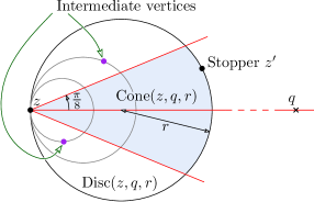
Figure 1: Choosing the next vertex.

2 Algorithm and geometric properties

We consider the finite set of sites in general position (so that no three points of the domain are co-linear, and no four points are co-circular), $\mathbf{X}\subset\mathbb{R}^{2}$ contained within a compact convex domain $\mathcal{D}\subset\mathbb{R}^{2}$. Let $\operatorname{DT}(\mathbf{X})$ be the Delaunay triangulation of $\mathbf{X}$, which is the graph in which three sites $x,y,z\in\mathbf{X}$ form a triangle if and only if the disc with $x,y$ and $z$ on its boundary does not contain any site in $\mathbf{X}$. Given two points $z,q\in\mathbb{R}^{2}$ and a number $r\in\mathbb{R}$ we define $\operatorname{Disc}(z,q,r)$ to be the closed disc whose diameter spans $z$ and the point at a distance $2r$ from $z$ on the ray $zq$. Finally, we define $\operatorname{Cone}(z,q,r)$ to be the sub-region of $\operatorname{Disc}(z,q,r)$ contained within a closed cone of apex $z$, axis $zq$ and half angle $\frac{\pi}{8}$ (see Figure 1).

2.1 The cone walk algorithm

Given a site $z\in\mathbf{X}$ and a destination point $q\in\mathcal{D}$, we define one step of the cone walk algorithm by growing the region $\operatorname{Cone}(z,q,r)$ anchored at $z$ from $r=0$ until the first point $z^{\prime}\in\mathbf{X}$ is found such that the region is non-empty. Once $z^{\prime}$ has been determined, we refer to it as the stopper. We call the region $\operatorname{Cone}(z,q,r)$ for the given $r$ a search cone, and we call the associated disc $\operatorname{Disc}(z,q,r)$ the search disc (see Figure 1). The point $z^{\prime}$ is then selected as the anchor of a new search cone $\operatorname{Cone}(z^{\prime},q,\cdot)$ and the next step of the walk begins. See Figure 2 for an example run of the algorithm.

To find the stopper using only neighbour incidences in the Delaunay triangulation, we need only access vertices in a well-defined local neighbourhood of the search disc. Define the points $\mathbf{X}\cap\operatorname{Disc}(z,q,r)\setminus\{z,z^{\prime}\}$ to be the intermediate vertices. The algorithm finds the stopper at each step by gradually growing a disc anchored at $z$ in the direction of the destination, adding the neighbours of all vertices in $\mathbf{X}$ intersected along the way. This is achieved in practice by maintaining a series of candidate vertices initialised to the neighbours of $z$ and selecting amongst them the vertex defining the smallest search disc at each iteration. Each time we find a new vertex intersecting this disc, we check to see if it is contained within $\operatorname{Cone}(z,q,\infty)$. If it is, this point is the next stopper and this step is finished. Otherwise the point must be an intermediate vertex and we add its neighbours to the list of candidate vertices. This procedure works because the intermediate vertex defining the next largest disc is always a neighbour of one of the intermediate vertices that we have already visited during the current step (see Lemma 5).

We terminate the algorithm when the destination $q$ is contained within the current search disc for a given step. At this point we know that one of the points contained within $\operatorname{Disc}(z,q,r)$ is a Delaunay neighbour of $q$ in $\operatorname{DT}(\mathbf{X}\cup\{q\})$. We can further compute the triangle of $\operatorname{DT}(\mathbf{X})$ containing the query point $q$ (point location) or find the nearest neighbour of $q$ in $\operatorname{DT}(\mathbf{X})$ by simulating the insertion of the point $q$ into $\operatorname{DT}(\mathbf{X})$ and performing an exhaustive search on the neighbours of $q$ in $\operatorname{DT}(\mathbf{X}\cup\{q\})$.

We will sometimes distinguish between the visited vertices, which we take to be the set of all sites contained within the search discs for every step and the accessed vertices, which we define to be the set of all vertices accessed by the cone-walk algorithm. Thus the accessed vertices are the visited vertices along with their 1-hop neighbourhood.

The pseudo-code below gives a detailed algorithmic description of the Cone-Walk algorithm. We take as input some $z\in\mathbf{X}$, $q\in\mathcal{D}$ and return a Delaunay neighbour of $q$ in $\operatorname{DT}(\mathbf{X}\cup\{q\})$. Recalling that $\mathbf{N}_{1}(v)$ refers to the Delaunay neighbours of $v\in\operatorname{DT}(\mathbf{X})$ and additionally defining $\textnormal{Next-Vertex}(S,z,q)$ to be the procedure that returns the vertex in $S$ with the smallest $r$ such that $\operatorname{Disc}(z,q,r)$ touches a vertex in $S$ and $\textnormal{In-Cone}(z,q,y)$ to be true when $y\in\operatorname{Cone}(z,q,\infty)$.

• $\textnormal{Cone-Walk}(z,q)$
       1$Substeps\mathrel{\hskip 1.0pt=\hskip 1.0pt}\{z\}$ 2$Candidates\mathrel{\hskip 1.0pt=\hskip 1.0pt}\mathbf{N}_{1}(z)$ 3while true 4 $y\mathrel{\hskip 1.0pt=\hskip 1.0pt}\textnormal{Next-Vertex}(Candidates\cup\{q\},z,q)$ 5 if $\textnormal{In-Cone}(z,q,y)$ 6 if $y=q$ 7 // Destination reached. 8 $\textbf{return}\;\textnormal{Next-Vertex}(Substeps,q,z)$ 9 // $y$ is a stopper 10 $z\mathrel{\hskip 1.0pt=\hskip 1.0pt}y$ 11 $Substeps\mathrel{\hskip 1.0pt=\hskip 1.0pt}\{z\}$ 12 $Candidates\mathrel{\hskip 1.0pt=\hskip 1.0pt}\mathbf{N}_{1}(z)$ 13 else 14 // $y$ is an intermediate vertex. 15 $Substeps\mathrel{\hskip 1.0pt=\hskip 1.0pt}Substeps\cup\{y\}$ 16 $Candidates\mathrel{\hskip 1.0pt=\hskip 1.0pt}Candidates\cup\mathbf{N}_{1}(y)\setminus Substeps$

2.2 Path Generation

We note that the order in which the vertices are discovered during the walk does not necessarily define a path in $\operatorname{DT}(\mathbf{X})$. If we only wish to find a point of the triangulation that is close to the destination (for example, in point location), this is not a problem. However, in the case of routing, a path in the triangulation is required to provide a route for data packets. To this end, we provide two options that we shall refer to as Simple-Path and Competitive-Path. Simple-Path is a simple heuristic that can quickly generate a path that is provably short on average. We conjecture that Simple-Path is indeed competitive, however we were unable to prove this. Competitive-Path is slightly more complex from an implementation point of view, however we show that for any possible input the algorithm will always generate a path of constant competitiveness whilst still maintaining the same asymptotic behaviour under the point distribution hypotheses explored in Section 3.

Simple-Path

A simple way to generate a valid path is to keep a predecessor table for each vertex. We start with an empty table at the beginning of each step, and then every time we access a new vertex, we store it in the table along with the vertex that we accessed it from. To trace a path back, we simply follow the predecessors.

Competitive-Path

Let $Z_{i}$ for $i>0$, be the $i$th stopper in the walk thus, $Z_{i}$ is the stopper found at step $i$) and $Z_{0}:=z$. For a path to be competitive, it should at least be locally competitive: for each step, there should be a bound on the length of the path generated between $Z_{i}$ and $Z_{i+1}$, which does not depend on the points in the search disc. To construct a path verifying this property, we use the fact that the stretch factor of the Delaunay triangulation is bounded above by a constant, $\lambda$. This means that for any two sites $x,y$, there exists a path from $x$ to $y$ in the Delaunay triangulation for which the sum of the lengths of the edges is at most $\lambda\|xy\|$. Currently the literature gives us that the stretch factor is in $[1.5932,1.998]$ [25, 26]. Clearly this implies that there exists a path between $Z_{i}$ and $Z_{i+1}$ with total length at most $\lambda\|Z_{i}Z_{i+1}\|$, and this path cannot exit the ellipse $\operatorname{Ell}(Z_{i},Z_{i+1}):=\{x\in\mathbf{X}:\|xZ_{i}\|+\|xZ_{i+1}\|<\lambda\|Z_{i}Z_{i+1}\|\}$. We use Dijkstra’s algorithm to find the shortest path between $Z_{i}$ and $Z_{i+1}$ which uses only vertices within $\operatorname{Ell}(Z_{i},Z_{i+1})$. The resulting path implicitly has stretch bounded by $\lambda$. We show in Lemma 4 that this algorithm results in a bound for the competitiveness for the full path.

Lemma 4.

Cone-Walk is $3.7$-competitive when the Competitive-Path algorithm is used to generate the path in $\operatorname{DT}(\mathbf{X})$

Proof.

Let $Z_{i}$, $Z_{i+1}$ be the stoppers of two consecutive steps defined by the algorithm. The stretch factor bound guarantees that the path generated between $Z_{i}$ and $Z_{i+1}$ has length bounded by $\lambda\|Z_{i}Z_{i+1}\|$, meaning that the longest path can have stretch at most $\lambda\sum_{i=0}^{\tau-1}\|Z_{i}Z_{i+1}\|/\|zq\|$ where $\tau$ is the number of steps in the walk. We bound this sum by observing that $\|Z_{i}Z_{i+1}\|\leq 2\cos\tfrac{\pi}{8}\cdot(\|Z_{i}q\|-\|Z_{i+1}q\|)$, which follows from Figure 8. Finally, no path defined by the algorithm can be longer than

$$\lambda\sum_{i=0}^{\tau-1}\|Z_{i}Z_{i+1}\|\leq 2\lambda\cos\tfrac{\pi}{8}\sum_{i=0}^{\tau-1}\big{(}\|Z_{i}q\|-\|Z_{i+1}q\|\big{)}\leq 2\lambda\cos\tfrac{\pi}{8}\cdot\|zq\|$$

Thus the path is $c$-competitive for $c:=2\lambda\cos\tfrac{\pi}{8}\leq 4\cos\tfrac{\pi}{8}\leq 3.7$. ∎

2.3 Complexity

In this section we give deterministic bounds on the number of operations required to compute $\textnormal{Cone-Walk}(z,q)$ within the RAM model of computation. In this model, accessing, comparing and performing arithmetic on points is treated as atomic. We will use these deterministic bounds to extract probabilistic bounds under certain distribution assumptions in Section 3.4. For now, we focus on a single step of the walk starting from $y\in\mathbf{X}$, and resulting in a disc with radius $r$. Let $k$ be the number of points intersecting the disc $\operatorname{Disc}(y,q,r)$ and $m$ be the number of edges in $\operatorname{DT}(\mathbf{X})$ intersecting $\partial\operatorname{Disc}(y,q,r)$ (where we use the notation $\partial A$ to denote the boundary of $A$) .

We note that every intermediate vertex will add its neighbours to the list of $Candidates$ when visited. Each of these insertions can be associated with a single edge of $\operatorname{DT}(X)$ intersecting $\operatorname{Disc}(y,q,r)$ (with multiplicity two for each ‘internal’ edge, since they are accessed from both sides). By the Euler relation, the total number of such insertions for one step is thus at most $3(m+2k)$. In addition, we observe that when moving from one intermediate vertex to the next, a search in the list of $Candidates$ is required. A simple linear search requires $O(m+k)$ operations for each intermediate vertex. Combining this with the above, we achieve a bound of $O(k(m+k))$ operations for one step. This bound may be improved by replacing $Candidates$ with a priority queue keyed on the associated search-disc radius of each candidate, which yields a simple improvement to $O(k\log(m+k))$.

For the path generation algorithms, we observe that Simple-Path only requires a constant amount of processing per vertex accessed to generate the predecessor table and $O(k)$ time to output the path at the end of each step, so the asymptotic running time is not affected by its inclusion. Competitive-Path is slightly more complicated since it accesses all points within an ellipse enclosing each search disc. Let $k^{\prime}$ be the number of points in this ellipse along with their neighbours. The path is found by applying Dijkstra’s algorithm to $k^{\prime}$ points, applying Euler’s relation gives us an updated bound for a single step of $O(k^{\prime}\log k^{\prime})$.

Figure 2: An example of cone walk. The points $(Z_{i})_{i>0}$ are the stoppers (or sometimes, the steps) and the points within each circle are the intermediate vertices. The shaded conic regions are the cones, and the set of outer circles for each of the steps in the diagram is referred to as the discs.

2.4 Geometric properties

We now prove a series of geometric lemmata giving properties of steps in the walk. We begin with a small lemma that will guarantee that we never get ‘stuck’ when performing a search for the next step, thus demonstrating correctness of the algorithm. The following two ‘overlapping’ lemmata allow us to establish which regions may be considered independent in a probabilistic sense and will be important in Section 3. Finally we provide a ‘stability’ result, which will help us to bound the region in which a destination point may be moved without changing the sequence of steps taken by the algorithm. This will be important when we enumerate the number of different walks possible for a given set of input points.

2.4.1 Finding a Delaunay path within the discs

Lemma 5 (Path finding lemma).

Let $q\in\mathcal{D}$, $z\in\mathbf{X}$ and $y^{\prime}\in\mathbf{X}$ with associated disc $\operatorname{Disc}(z,q,r^{\prime})$. Suppose there exists an $r>0$ such that $\left(\operatorname{Disc}(z,q,r^{\prime})\setminus\operatorname{Disc}(z,q,r)\right)\cap\mathbf{X}=\{y^{\prime}\}$. Then there exists a point in $\operatorname{Disc}(z,q,r)$ that is a Delaunay neighbour of $y^{\prime}$.

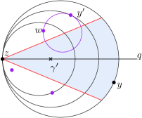
Figure 3: We observe that $y^{\prime}$ has always a Delaunay neighbour in $\operatorname{Disc}(z,q,r)$, where $r$ is the radius ensuring $y\in\partial\!\operatorname{Disc}(z,q,r)$.

Proof.

Let $\gamma^{\prime}$ be the centre of $\operatorname{Disc}(z,q,r^{\prime})$. We grow $\operatorname{Disc}(y^{\prime},\gamma^{\prime},\rho)\subset\operatorname{Disc}(z,q,r^{\prime})$ until we hit a point $w$ in $\mathbf{X}$. The point $w$ is always contained within $\operatorname{Disc}(z,q,r)$ because $z$ is on the border of $\operatorname{Disc}(z,q,r)$. Since the interior of the $\operatorname{Disc}(y^{\prime},\gamma^{\prime},\rho)$ is empty, $w$ is a Delaunay neighbour of $y^{\prime}$. See Figure 3. ∎

Corollary 6.

Let $q\in\mathcal{D}$, $z\in\mathbf{X}$ with $y\in\mathbf{X}$ its associated stopper satisfying $y\in\partial\!\operatorname{Cone}(z,q,r)$. Then there is a path of edges of   $\operatorname{DT}(\mathbf{X})$ between $z$ and $y$ contained within $\operatorname{Disc}(z,q,r)$.

2.4.2 Independence of the search cones

When growing a new search cone, it is important to observe that it does not overlap any of the previous search cones, except at the very end of the walk. This is formalised by the following lemma.

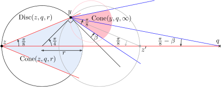
Figure 4: For the proof of Lemma 7.

Lemma 7 (Non-overlapping lemma).

Let $z$ and $y$ be two points of  $\mathbf{X}$ and $r>0$ such that $\operatorname{Cone}(z,q,r)$ has $y$ on its boundary. If $\|zq\|>(2+\sqrt{2}\,)r$ then $\operatorname{Disc}(z,q,r)$ does not intersect the search cone $\operatorname{Cone}(y,q,\infty)$ issued from $y$ nor any other search cone for any subsequent step of the walk.

Proof.

Assume without loss of generality that $y$ lies to the left of line $zq$ and consider the construction given in Figure 4. Let $\beta$ denote the angle between the tangent to $\operatorname{Disc}(z,q,r)$ at $y$ and the ray bordering $\operatorname{Cone}(y,q,\infty)$. $\operatorname{Cone}(y,q,\infty)$ and $\operatorname{Disc}(z,q,r)$ do not intersect provided that $\beta\geq 0$. Placing $y$ at the corner of $\operatorname{Cone}(z,q,r)$ maximizes $\beta$, in which case we have $\beta>0$ if and only if $q$ is to the right of $z^{\prime}$, the point symmetrical to $z$ with respect to the line through $y$ perpendicular to $zq$. Elementary computations then yield the result. Since the whole sequence of search cones following the one issued from $y$ remains in $\operatorname{Cone}(y,q,\infty)$, $\operatorname{Disc}(z,q,r)$ does not intersect any of these search cones, and the result follows. ∎

2.4.3 Independence of the search discs

When growing the search disc region, the new search disc may overlap previous search discs but only in their cone parts. This is formalised by the following lemma:

Lemma 8 (Overlapping lemma).

Let $z$ and $y$ be two points such that $\operatorname{Cone}(z,q,r)$ has $y$ on its boundary. Then if the search disc $\operatorname{Disc}(y,q,\rho)$ issued from $y$ does not contain $q$, it does not intersect $\operatorname{Disc}(z,q,r)\setminus\operatorname{Cone}(z,q,r)$.

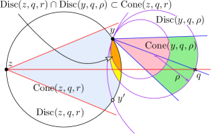
Figure 5: For the proof of Lemma 8.

Proof.

By symmetry we observe that $\operatorname{Disc}(y,q,\rho)$ only intersects the point $y^{\prime}$, the point $y$ reflected through the line $zq$, when the centre of $\operatorname{Disc}(y,q,\rho)$ coincides with $q$ Figure 5). Since the algorithm terminates as soon as the current search disc touches $q$, $q$ is never contained within $\operatorname{Disc}(z,q,\rho)$ and thus this can never happen. ∎

2.4.4 Stability of the walk

In the following lemma we are interested in the stability of the sequence of steps to reach $q$.

Lemma 9 (Invariance lemma).

For an $n$-set $\mathbf{X}\subseteq\mathbb{R}^{2}$, there exists an arrangement of half-lines $\Xi=\Xi(\mathbf{X})$ such that the associated subdivision of the plane has fewer than $2n^{4}$ cells, and such that the sequence of steps used by the cone walk algorithm from any vertex of $\mathbf{X}$ does not change when the aim $q$ moves in a connected component of $\mathbb{R}^{2}\setminus\Xi$.

Figure 6: For the proof of Lemma 9. For a given step $z$, moving the destination in the shaded sector will always result in the same stopper, $s$, being chosen for the next step.

Proof.

Take a point $z\in\mathbf{X}$ and consider $\mathcal{S}_{z}$, the set of all possible stoppers defined by $\operatorname{Cone}(z,q,r)$ for some $q\in\mathcal{D}$ and $r>0$. Each $s\in\mathcal{S}_{z}$ defines a unique sector about $z$ such that moving a point in the given sector does not change the stopper (see Figure 6). We then create an arrangement by adding a ray on the border of every sector for each point $z\in\mathbf{X}$. The resulting arrangement has the property that moving the destination point $q$ within one of the cells of the arrangement does not change the stopper of any step for any possible walk. Clearly, $|\mathcal{S}_{z}|\leq n-1$ for all $z\in\mathbf{X}$, and each sector is bounded by at most two rays, thus there are at most $2n(n-1)$ rays in the arrangement. Since an arrangement of $m$ lines has at most $\frac{m^{2}+m+2}{2}$ cells the result follows [see, e.g., 20, p. 127]. ∎

3 Cone walk on Poisson Delaunay in a disc

Our aim in this section is to prove the main elements towards Theorem 3, which we go on to complete in Section 4. Our ultimate goal is to prove bounds on the behaviour of the cone walk for the worst possible pair of starting point and query when the input sites are generated by a homogeneous Poisson process in a compact convex domain. Achieving this requires first strong bounds on the probability that the walk behaves badly for a fixed start point and query. One then proves the worst-case bounds by showing that to control every possible run of the algorithm, it suffices to bound the behaviour of the walk for enough pairs of starting points and query; this relies crucially on the arrangement of Lemma 9. The tail bounds required in the second stage of the proof may not be obtained from Markov or Chebyshev’s inequalities together with mean or variance estimates only, and we thus need to resort to stronger tools.

Our techniques rely on concentration inequalities [15, 9, 21, 16]. Most of the bounds we obtain (for the number of steps $\kappa$ and the number of visited sites) follow from a representation as a sum of random variables in which the increments can be made independent by a simple and natural conditioning. The bounds on the complexity of the algorithm Cone-Walk are slightly trickier to derive because there is no way to make the increments independent.

For the sake of presentation, we introduce two simplifications which we remove in Section 4. First, we start by studying the walk in the disc $\mathcal{D}_{n}$ of area $n$ where the query is at the centre. These choices for $\mathcal{D}_{n}$ and $q$ ensure that for any $z\in\mathcal{D}_{n}$ and any $r\leq\sqrt{n/\pi},$ we have $\operatorname{Disc}(z,q,r)\subset\mathcal{D}_{n}$. Note that since the distance to the aim is decreasing, the disc is precisely the effective domain where the walk from $z$ and aiming at $q$ takes place.

Then, we introduce independence between the different regions of the domain by replacing the collection of independent points $\mathbf{X}_{n}$ by a (homogeneous) Poisson point process $\mathbf{\Phi}$ and consider $\operatorname{DT}(\mathbf{\Phi})$. Recall that a Poisson point process of intensity $1$ is a random collection of points $\mathbf{\Phi}\subset\mathcal{D}_{n}$ such that with probability one, all the points are distinct, for any two Borel sets $R,S\subseteq\mathcal{D}_{n}$, the number of points $|\mathbf{\Phi}\cap R|$ is distributed like a Poisson random variable whose mean is the area $\mathcal{A}(R)$ of $R$, and if $R\cap S=\varnothing$ then $|\mathbf{\Phi}\cap R|$ and $|\mathbf{\Phi}\cap S|$ are independent.

On many occasions, it is convenient to consider $\mathbf{\Phi}$ conditioned to have a point located at $z\in\mathcal{D}$ and we let $\mathbf{\Phi}_{z}$ be the corresponding random point set. Classical results on Poisson point processes ensure that $\mathbf{\Phi}_{z}\setminus\{z\}$ is distributed like $\mathbf{\Phi}$, so that one can take $\mathbf{\Phi}_{z}=\mathbf{\Phi}\cup\{z\}$, for $\mathbf{\Phi}$ independent of $z$ [see, e.g., 1, Section 1.4].

3.1 Preliminaries

We establish the following notation (see Figure 2). Let ${\mathbf{Z}}=(Z_{i},i>0)$ denote the sequence of stoppers visited during the walk with $Z_{0}:=z$. Let $L_{i}=\|Z_{i}q\|$ denote the distance to the destination $q$. The distance $L_{i}$ is strictly decreasing and the point set $\mathbf{\Phi}$ is almost surely finite, thus ensuring that the walk stops after a finite number of steps $\kappa$, at which point we have $Z_{\kappa}=q$. For $x>0$, we also let $\kappa(x)$ be the number of steps required to reach a point within distance $x$ of the query. Therefore $i<\kappa(x)$ if and only if $L_{i}>x$. The important parameters needed to track the location and progress of the walk are the radius $R_{i}$ such that $Z_{i+1}\in\partial\!\operatorname{Cone}(Z_{i},q,R_{i})$, and the angle $\alpha_{i}$ between $Z_{i}q$ and $Z_{i}Z_{i+1}$. $\operatorname{Disc}(Z_{i},q,R_{i})$ may contain several points of $\mathbf{\Phi}$, let $\tau_{i}$ denote $|\operatorname{Disc}(Z_{i},q,R_{i})\setminus\{Z_{i},Z_{i+1}\}\cap{\mathbf{\Phi}}|$ the number of such points and $N_{i}$ the number of these points along with their Delaunay neighbours.

In order to compute the walk efficiently, the algorithm presented gathers a lot of information. In particular, we access all of the points in $\operatorname{Disc}(Z_{i},q,R_{i})$ and their neighbours. For the analysis, we want to keep the landscape as concise as possible, and so we define a filtration which only contains the necessary information for the walk to be a measurable process. Let $\mathcal{F}_{i}$ denote the information consisting of (the $\sigma$-algebra generated by) the locations of the points of $\mathbf{\Phi}$ contained in $\cup_{j=0}^{i}\operatorname{Disc}(Z_{j},q,R_{j})$. Finally, we shall write $\omega_{n}$ to denote a sequence satisfying $\omega_{n}\geq\log n$.

We often need to condition on the size of the largest empty ball within the process $\mathbf{\Phi}_{n}$. This is dealt with in the following lemma.

Lemma 10.

Let $b(\mathbf{x},r)$ denote the closed ball of radius $r$ centred at $\mathbf{x}$. Then $\forall c>0$, $\xi>0$,

$$\mathbb{P}\big{(}\exists x\in\mathcal{D}_{n}:b(x,c\,\omega_{n}^{1/2+\xi})\cap\mathbf{\Phi}_{n}=\varnothing\big{)}\leq\exp\left(-\omega_{n}^{1+\xi}\right)$$

for $n$ sufficiently large.

Proof.

We have

$$\mathbb{P}(\exists x\in\mathcal{D}_{n}:b(x,c\,\omega_{n}^{1/2+\xi})\cap\mathbf{\Phi}_{n}=\varnothing) \leq\mathbb{P}(\exists B\in P:B\cap\mathbf{\Phi}_{n}=\varnothing),$$

where $P$ is any maximal packing of $\mathcal{D}$ with balls $B$ of radius $\frac{1}{2}c\,\omega_{n}^{1/2+\xi}$ centred in $\mathcal{D}_{n}$. If the radius of curvature of $\mathcal{D}_{n}$ is lower bounded by $c\,\omega_{n}^{1/2+\xi}$ (which happen for $n$ largr enough) such a ball $B$ contains a ball of radius $\frac{1}{4}c\,\omega_{n}^{1/2+\xi}$ entirely inside $\mathcal{D}_{n}$, For $n$ large enough, any such packing contains at most $n$ balls and we have

$$\mathbb{P}(\exists x\in\mathcal{D}_{n}:b(x,c\,\omega_{n}^{1/2+\xi})\cap\mathbf{\Phi}_{n}=\varnothing)\leq n\exp\left(-\pi\tfrac{1}{4^{2}}\right)c^{2}\omega_{n}^{1+2\xi}\leq\exp\left(-\omega_{n}^{1+\xi}\right).\qed$$

3.1.1 The size of the discs

If the search cone $\operatorname{Cone}(Z_{i},q,\infty)$ does not intersect any of the previous discs, the region which determines $R_{i+1}$ is ‘fresh’ and $R_{i+1}$ is independent of $\mathcal{F}_{i}$. Lemma 7 provides a condition which guarantees independence of the search cones. To take advantage of it, we write $\xi:=2+\sqrt{2}$, and for $i\geq 0$, define the event

$$G_{i}:=\{\forall j\leq i+1,R_{j}<\omega_{n}/\xi\},$$ (1)

Then if the event $G_{i}^{\star}:=G_{i}\cap\{L_{i}\geq\omega_{n}\}$ occurs; for every $j\leq i$, the search-cone $\operatorname{Cone}(Z_{j},q,\infty)$ does not intersect any of the regions $\operatorname{Disc}(Z_{k},q,R_{k})$, $0\leq k<j$, and the corresponding variables $(R_{j},\alpha_{j})$, $0\leq j\leq i+1$ are independent. Although it might seem like an odd idea, $G_{i}^{\star}$ does include some condition on $R_{i+1}$; this ensures that on $G_{i}^{\star}$, we have $L_{i+1}>L_{i}-2R_{i+1}>0$, so that $i+1$ is not the last step. So for $x>0$ we have

$$\mathbb{P}(R_{i+1}>x\,|\,\mathcal{F}_{i},G_{i}^{\star}) =\mathbb{P}(\mathbf{\Phi}\cap\operatorname{Cone}(Z_{i},q,x)\setminus\{Z_{i}\}=\varnothing\,|\,\mathcal{F}_{i},G_{i}^{\star})\mathbf{1}_{\{\xi x\leq\omega_{n}\}}$$

$$=\exp\left(-Ax^{2}\right)\mathbf{1}_{\{\xi x\leq\omega_{n}\}},$$ (2)

where $A$ denotes the area of $\operatorname{Cone}(z,q,1)$ which is the shaded region in Figure 1. Indeed, conditional on $\mathcal{F}_{i}$ and $G_{i}^{\star}$, $|\mathbf{\Phi}\cap\operatorname{Cone}(Z_{i},q,x)\setminus\{Z_{i}\}|$ is a Poisson random variable with mean $Ax^{2}$ where

$$A:=2\left(\cos\frac{\pi}{8}\sin\frac{\pi}{8}+\frac{\pi}{8}\right)=\frac{\sqrt{2}}{2}+\frac{\pi}{4}.$$ (3)

We will repeatedly use the conditioning on $G_{i}$ to introduce independence, and it is important to verify that $G_{i}$ indeed occurs with high probability. For $G_{i}$ to fail, there must be a first step $j$ for which $R_{j}\geq\omega_{n}/\xi$. Writing $G_{i}^{c}$ for the complement of $G_{i}$ and defining $G_{-1}$ to be a void conditioning: provided that $i=O(n)$ (which will always be the case in the following)

$$\mathbb{P}(G_{i}^{c}) \leq\sum_{0\leq j\leq i+1}\mathbb{P}(R_{j}\geq\omega_{n}/\xi\,|\,G_{j-1})$$

$$\;\;\leq\exp\left(\log O(n)-A\omega_{n}^{2}/\xi^{2}\right)$$

$$\;\;\leq\exp\left(-\omega_{n}^{3/2}\right)$$ (4)

for all $n$ large enough since $\omega_{n}\geq\log n$.

Remark about the notation. It is convenient to work with an “ideal” random variable that is not constrained by the location of the query or artificially forced to be at most $\omega_{n}/\xi$, and we define $\mathcal{R}$ by $\mathbb{P}(\mathcal{R}\geq x)=\exp\left(-Ax^{2}\right)$ for $x\geq 0$. In the course of the proof, we use multiple other such ideal random variables, to distinguish them from the ones arising from the actual process, we use calligraphic letters to denote them.

3.1.2 The progress for one step

We now focus on the distribution of the angle $\angle qZ_{i}Z_{i+1}$ and by extension the progress made during one step in the walk. Let $\operatorname{Cone}_{\alpha}(z,q,r)$ be the cone of half angle $\alpha$ with the same apex and axis as $\operatorname{Cone}(z,q,r)$. For $S\subset\mathbb{R}^{2}$, let $\mathcal{A}(S)$ denote its area. On the event $G_{i}^{\star}$, $Z_{i+1}\neq q$ and $\alpha_{i+1}$ is truly random and its distribution is symmetric and given by (see Figure 7):

$$\mathbb{P}(|\alpha_{i+1}|<x\;|\;R_{i+1}=r,\mathcal{F}_{i},G_{i}^{\star}) =\lim_{\varepsilon\to 0}\frac{\mathcal{A}(\operatorname{Cone}_{x}(Z_{i},q,r+\varepsilon)\setminus\operatorname{Cone}_{x}(Z_{i},q,r))}{\mathcal{A}(\operatorname{Cone}(Z_{i},q,r+\varepsilon)\setminus\operatorname{Cone}(Z_{i},q,r))}$$

$$=\lim_{\varepsilon\rightarrow 0}\frac{((r+\varepsilon)^{2}-r^{2})(x+\frac{1}{2}\sin 2x)}{((r+\varepsilon)^{2}-r^{2})(\frac{\pi}{8}+\frac{\sqrt{2}}{4})}$$

$$=\frac{8}{\pi+2\sqrt{2}}\left(x+\frac{\sin 2x}{2}\right).$$ (5)

So in particular, conditional on $\mathcal{F}_{i}$ and $G_{i}^{\star}$, $\alpha_{i+1}$ is independent of $R_{i+1}$. We will write $\alpha$ for the ‘ideal’ angle distribution given by (3.1.2), and enforce that $\mathcal{R}$ and $\alpha$ be independent.

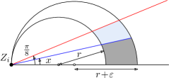
Figure 7: For the angle to be smaller than $x$ given $R_{i+1}\in[r,r+\varepsilon]$, the stopper must fall within the dark shaded region

3.2 Geometric and combinatorial parameters

In this section we will build the elements required to bound the algorithmic complexity of the Cone-Walk algorithm. We begin by bounding the number of steps (or equivalently, the number of stoppers) required by the walk process to reach the destination. We will then bound the number of vertices visited by the walk process, recalling that this will involve bounding the number of intermediary vertices within the discs $\operatorname{Disc}(Z_{i},q,R_{i})$ at each step. The final part of the proof will be to bound the number of vertices accessed by the Cone-Walk algorithm when constructing the sequence of stoppers and intermediary vertices. The vertices accessed will include all of the vertices visited, and their 1-hop neighbourhood.

3.2.1 The maximum number of vertices accessed during a step

At each step during a walk, we do not a priori access a bounded number of sites when performing a search for the next stopper. Such a bound is important to limit the number of neighbourhoods that may be accessed during one step, since we note that the maximum number of vertices accessed during one step explicitly provides an upper bound on the number of neighbourhoods accessed. A easy bound of $\log^{1+\varepsilon}n$, for any $\varepsilon>0$ may be obtained when considering pairs of start and destination points at least $\sqrt{\log n}$ away from the border of $\partial\mathcal{D}$. However, we opt to explicitly take care of border effects, giving us a slightly weaker bound that can be applied everywhere.

Proposition 11.

Let $M_{\text{max}}$ be the maximum number of vertices accessed during any step in any walk. Then

$$\mathbb{P}\bigg{(}M_{\text{max}}\geq\omega_{n}^{3+\xi}\bigg{)}\leq 2\exp\left(-\omega_{n}^{1+\xi/4}\right).$$

In the following, we note that $M_{\text{max}}$ is bounded by $\tau_{\text{max}}\cdot\Delta_{\mathbf{\Phi}}$, where $\Delta_{\mathbf{\Phi}}$ gives the maximum degree of any vertex contained within $\operatorname{DT}(\mathbf{\Phi})$ and $\tau_{\text{max}}$ is the maximum number sites contained within any step in any instance of cone walk. We thus focus on bounding $\tau_{\text{max}}$, and our result will follow directly from the proof of Proposition 30 in Appendix A.

Lemma 12.

$$\mathbb{P}(\tau_{\text{max}}>\omega^{1+\xi}_{n})\leq\exp\left(-\omega_{n}^{1+\xi/3}\right).$$

Proof.

Let $A$ be the event that the maximum disc radius for any step in any walk is bounded by $\tfrac{1}{2}\omega_{n}^{1/2+\xi}$ and let $B$ be the event that every ball $b(x,\tfrac{1}{2}\omega_{n}^{1/2+\xi})$ contains fewer than $\omega_{n}^{1+2\xi}$ points of $\mathbf{\Phi}$, for $x\in\mathcal{D}$. We have, for $n$ large enough,

$$\mathbb{P}(\tau_{\text{max}}>\omega^{1+2\xi}_{n}) \leq\mathbb{P}(\tau_{max}>\omega_{n}^{1+2\xi}\mid A\cap B)+\mathbb{P}(A^{c})+\mathbb{P}(B^{c})$$

$$\leq\exp\left(-\omega_{n}^{1+\xi}\right)+\exp\left(-\omega_{n}^{1+\xi}\right).$$

Note that the bound on $\mathbb{P}(A^{c})$ is implied by Lemma 10 since a large disc implicitly has a large empty cone. For the bound on $\mathbb{P}(B^{c})$, we imagine splitting $\mathcal{D}$ into a uniform grid with squares of side $\tfrac{1}{2}\omega_{n}^{1+\xi}$. The proof follows by noting that every ball of radius $\tfrac{1}{2}\omega_{n}^{1+\xi}$ is contained in a group of at most four adjacent squares, each of which must contain at least $\tfrac{1}{4}\omega^{1+2\xi}_{n}$ sites. We then use the fact that $n\mathbb{P}(\operatorname{Po}(\tfrac{1}{4}\omega_{n}^{1+\xi})\geq\frac{1}{4}\omega_{n}^{1+2\xi})\leq\exp\left(-\omega_{n}^{1+\xi}\right)$ for $n$ large enough. We omit the details. ∎

3.2.2 The number of steps in the walk

Recall that a new step is defined each time a new stopper is visited. We will start with a first crude estimate for the decrease in distance after a given number of steps. Note that $L_{i}=\|Z_{i}q\|$ and $\alpha_{i}$ denotes the angle between $Z_{i}Z_{i+1}$ and $Z_{i}q$. Simple geometry implies (see Figure 8):

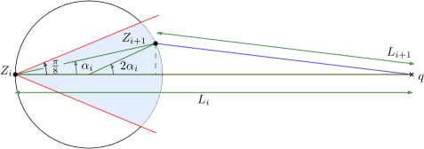
Figure 8: Computing distance progress at step $i$.

$$L_{i}-R_{i}(1+\cos(2\alpha_{i}))\leq L_{i+1} =\sqrt{(L_{i}-R_{i}(1+\cos(2\alpha_{i})))^{2}+R_{i}^{2}\sin^{2}(2\alpha_{i})}$$

$$\leq L_{i}-R_{i}(1+\cos(2\alpha_{i}))+2\frac{R_{i}^{2}}{L_{i}},$$ (6)

since $\sqrt{1-x}\leq 1-x/2$ for any $x\in[0,1]$. As a consequence

$$L_{0}-\sum_{j=0}^{i-1}R_{i}(1+\cos(2\alpha_{i}))\leq L_{i} \leq L_{0}-\sum_{j=0}^{i-1}R_{i}(1+\cos(2\alpha_{i}))+\frac{2}{\omega_{n}}\cdot\sum_{j=0}^{i-1}R_{i}^{2}.$$ (7)

In particular, since $\omega_{n}\to\infty$, after $i$ steps, the expected distance $\mathbb{E}[L_{i}]$ to the aim $q$ should not be far from $L_{0}-i\mathbb{E}[\mathcal{R}(1+\cos(2\alpha))].$ Furthermore, conditional on $G_{i}$, and for $i$ such that $L_{i}\geq\omega_{n}$, the summands involved in Equation (7) are independent, bounded by $2\omega_{n}$ and have bounded variance, so that the sum should be highly concentrated about its expected value [15, 9, 21]. In other words, one expects that for $i$ much larger than $L_{0}/\mathbb{E}[\mathcal{R}(1+\cos 2\alpha)]$, it should be the case that $L_{i}\leq\omega_{n}$ with fairly high probability. Making this formal constitutes the backbone of our proof.

Lemma 13.

Let $z\in\mathcal{D}$, suppose that $\ell\geq 1$ is such that $L_{0}=\|zq\|\geq(\ell+1)\omega_{n}$. Consider $\operatorname{DT}(\mathbf{\Phi}_{z})$. There exists a constant $\eta>0$ such that

$$\mathbb{P}\left(L_{0}-L_{\ell}\leq\ell\,\mathbb{E}[\mathcal{R}]/2\right)\leq\exp\left(-\eta\ell/\omega_{n}\right)+\exp\left(-\omega_{n}^{3/2}\right).$$

Proof.

We use the crude bounds $R_{i}\leq L_{i}-L_{i+1}\leq 2R_{i}$ (see Figure 8). It follows that

$$\mathbb{P}(L_{0}-L_{\ell}\leq\ell\,\mathbb{E}[\mathcal{R}]/2) \leq\mathbb{P}(L_{0}-L_{\ell}\leq\ell\,\mathbb{E}[\mathcal{R}]/2\,|\,G_{\ell})+\mathbb{P}(G_{\ell}^{c})$$

$$\leq\mathbb{P}\Bigg{(}\sum_{j=0}^{\ell-1}R_{j}\leq\frac{\ell}{2}\mathbb{E}[\mathcal{R}]\,\Bigg{|}\,G_{\ell}\Bigg{)}+\exp\left(-\omega_{n}^{3/2}\right),$$

by (3.1.1), since the constraint on $\ell$ imposes that $\ell=O(\sqrt{n}\,)$. Now, since $L_{0}\geq(\ell+1)\omega_{n}$ and $\xi>2$, on the event $G_{\ell}$, we have $L_{i}\geq\omega_{n}$ for $0\leq i\leq\ell$ so that $G_{\ell}^{\star}$ occurs: conditional on $G_{\ell}$, the search cones do not intersect and the random variables $R_{j}$, $0\leq j\leq\ell$ are independent and identically distributed (see Lemma 7). Furthermore, we have

$$\mathbb{E}[R_{j}\,|\,G_{\ell}] =\int_{0}^{\infty}\mathbb{P}\left(R_{j}\geq x\,|\,G_{\ell}\right)dx$$

$$\geq\int_{0}^{\omega_{n}/\xi}\exp\left(-Ax^{2}\right)dx$$

$$\geq\mathbb{E}[\mathcal{R}]-\exp\left(-\omega_{n}^{3/2}\right),$$

for all $n$ large enough. It follows that for all $n$ large enough, by Theorem 2.7 of [21, p. 203]

$$\mathbb{P}\Bigg{(}\sum_{j=0}^{\ell-1}R_{j}\leq\frac{\ell}{2}\mathbb{E}[\mathcal{R}]\,\bigg{|}\,G_{\ell}\Bigg{)} \leq\mathbb{P}\Bigg{(}\sum_{j=0}^{\ell-1}(R_{j}-\mathbb{E}[R_{j}\,|\,G_{\ell}])\leq-\frac{\ell}{3}\mathbb{E}[R_{0}\,|\,G_{\ell}]\,\Bigg{|}\,G_{\ell}\Bigg{)}$$

$$\leq\exp\left(-\frac{t^{2}}{2\ell\,\mathbb{V}(R_{0}\,|\,G_{\ell})+2t\omega_{n}/3}\right)\qquad t=\ell\,\mathbb{E}[R_{0}\,|\,G_{\ell}]/3$$

$$\leq\exp\left(-\eta\ell/\omega_{n}\right),$$

for some constant $\eta>0$ independent of $\ell$ and $n$. ∎

The rough estimate in Lemma 13 may be significantly strengthened, and the very representation in (7) yields a bound on the number of search cones or steps that are required to get within distance $\omega_{n}$ of the query point $q$. (If the starting site $z$ satisfies $L_{0}=\|zq\|\leq\omega_{n}$, then this phase does not contain any step.)

Proposition 14.

Let $z\in\mathcal{D}_{n}$, and let $\kappa(\omega_{n})$ denote the number of steps of the walk to reach a site which is within distance $\omega_{n}$ of $q$ in $\mathbf{\Phi}_{z}\cup\{q\}$ when starting from the site $z\in\mathbf{\Phi}_{z}$ at distance $L_{0}=\|zq\|\geq\omega_{n}$. Then

$$\mathbb{P}\left(\left|\kappa(\omega_{n})-\frac{L_{0}}{\mathbb{E}[\mathcal{R}(1+\cos 2\alpha)]}\right|\geq 2\omega_{n}^{2}\sqrt{2L_{0}}+\omega_{n}\right)\leq 4\exp\left(-\omega_{n}^{3/2}\right).$$

Proof.

We now make formal the intuition that follow Equation (7). We start with the upper bound. For any integer $k\geq 0$, we have

$$\mathbb{P}\left(\kappa(\omega_{n})\geq k\right) =\mathbb{P}\left(L_{k}\geq\omega_{n}\right)$$

$$\leq\mathbb{P}\left(L_{k}\geq\omega_{n}\,|\,G_{k}\right)+\mathbb{P}\left(G_{k}^{c}\right),$$

and since the second term is bounded in (3.1.1), it now suffices to bound the first one. However, given $G_{k}$ and $L_{k}\geq\omega_{n}$, the random variables $(R_{i},\alpha_{i})$, $i=1,\dots,k$ are independent and identically distributed. The only effect of this conditioning is that $R_{i}$ is distributed as $\mathcal{R}$ conditioned on $\mathcal{R}<\omega_{n}/\xi$.

Write $X_{i}=R_{i}(1+\cos 2\alpha_{i})-2R_{i}^{2}/\omega_{n}$, and note that $X_{i}\geq 0$ if $R_{i}\leq\omega/\xi$. Then, from (7), we have

$$\mathbb{P}\left(L_{k}\geq\omega_{n}\,|\,G_{k}\right) \leq\mathbb{P}\left(\sum_{i=0}^{k-1}X_{i}\leq L_{0}-\omega_{n}\,\Bigg{|}\,G_{k},{L_{k}\geq\omega_{n}}\right).$$

Conditional on $G_{k}^{\star}=G_{k}\cap\{L_{k}\geq\omega_{n}\}$, the random variables $X_{i}$ are independent, $0\leq X_{i}\leq 2R_{i}\leq\omega_{n}$. Furthermore, since $X_{i}$ has Gaussian tails, its variance (conditional on $G_{k}$) is bounded by a constant independent of $i$ and $n$. Choosing $k_{0}=\lceil(L_{0}+t)/\mathbb{E}[X_{0}\,|\,G_{0}^{\star}]\rceil$, for some $t<L_{0}$ to be chosen later, and using the Bernstein-type inequality in Theorem 2.7 of [21, p. 203], we obtain

$$\mathbb{P}(L_{k_{0}}\geq\omega_{n}\,|\,G_{k_{0}}) \leq\mathbb{P}\left(\sum_{i=0}^{k_{0}-1}(X_{i}-\mathbb{E}[X_{i}\,|\,G_{k_{0}}])\leq-t\,\Bigg{|}\,G_{k_{0}}^{\star}\right)$$

$$\leq\exp\left(-\frac{t^{2}}{2k_{0}\mathbb{V}(X_{0}\,|\,G_{0}^{\star})+2\omega_{n}t/3}\right).$$

In particular, for $t=\omega_{n}^{3}\sqrt{L_{0}}$, we have for all $n$ large enough $\mathbb{P}\left(L_{k_{0}}\geq\omega_{n}\,|\,G_{k_{0}}\right)\leq\exp\left(-\omega_{n}^{2}\right)$, since $L_{0}\geq\omega_{n}$.

A matching lower bound on $\kappa(\omega_{n})$ may be obtained similarly, using the lower bound on $L_{i+1}$ in Equation (3.2.2) and following the approach we used to devise the upper bound with $X_{i}^{\prime}=R_{i}(1+\cos 2\alpha_{i})$ (we omit the details). It follows that, for $k_{1}=\lfloor(L_{0}+t)/\mathbb{E}[X_{0}^{\prime}\,|\,G_{0}^{\star}]\rfloor$, we have $\mathbb{P}(L_{k_{1}}\leq\omega_{n}\,|\,G_{k_{1}})\leq\exp\left(-\omega_{n}^{2}\right)$.

To complete the proof, it suffices to estimate the difference between $k_{0}$ and $k_{1}$. We have

$$\mathbb{E}[X_{0}\,|\,G_{0}^{\star}] =\mathbb{E}[R_{0}(1+\cos 2\alpha_{0})\,|\,G_{0}^{\star}]-\frac{2\mathbb{E}[R_{0}^{2}\,|\,G_{0}^{\star}]}{\omega_{n}}$$

$$=\mathbb{E}[\mathcal{R}(1+\cos 2\alpha)]+O(1/\omega_{n}),$$

and similarly, $\mathbb{E}[X_{0}^{\prime}\,|\,G_{0}^{\star}]=\mathbb{E}[\mathcal{R}(1+\cos 2\alpha)]$. It follows that $|k_{1}-k_{0}|=O(L_{0}/\omega_{n})$, which is not strong enough to prove the claim. So we need to strengthen the upper bound on the second sum in the right-hand side of (7). We quickly sketch how to obtain the required estimate. The idea is to use a dyadic argument to decompose $\kappa(\omega_{n})$ into the number of steps to reach $L_{0}/2^{j}$, for $j\geq 1$, until one gets to $\omega_{n}$ for $j=j_{0}:=\lceil\log_{2}(L_{0}/\omega_{n})\rceil$. For the steps $i$ which are taken from $Z_{i}$ with $L_{i}/L_{0}\in(2^{-j},2^{-j+1}]$, we use the improved bound

$$L_{i+1}\leq L_{i}-R_{i}(1+\cos 2\alpha)+\frac{2}{L_{0}2^{-j}}R_{i}^{2}.$$

Then write

$$\kappa(\omega_{n})=\sum_{j=1}^{j_{0}}\big{[}\kappa(L_{0}/2^{j})-\kappa(L_{0}/2^{j-1})\big{]},$$

and observe that the $j$-th summand is stochastically dominated by $\kappa(L_{0}^{\prime}/2)$ where $L_{0}^{\prime}=L_{0}/2^{j-1}$. For each $j$, we define $k_{0}(j)=\lceil(L_{0}/2^{j}+t_{j})/\mathbb{E}[X_{0}\,|\,G_{0}^{\star}]\rceil$ where $t_{j}:=\omega_{n}^{2}\sqrt{L_{0}/2^{j}}$ and note that

$$\sum_{j=1}^{j_{0}}k_{0}(j) \leq\frac{1}{\mathbb{E}[X_{0}\,|\,G_{0}^{\star}]}\sum_{j=1}^{j_{0}}(L_{0}/2^{j}+t_{j})+\lceil\log_{2}(L_{0}/\omega_{n})\rceil$$

$$\leq\frac{L_{0}}{\mathbb{E}[X_{0}\,|\,G_{0}^{\star}]}+2\omega_{n}^{2}\sqrt{2L_{0}}+\omega_{n},$$

for $\omega_{n}\geq\log n$, since $\pi L_{0}^{2}\leq n$. In other words, if $\kappa(L_{0}/2^{j})-\kappa(L_{0}/2^{j-1})\leq k_{0}(j)$ for every $j$, then $\kappa(\omega)\leq L_{0}/\mathbb{E}[X_{0}\,|\,G_{0}^{\star}]+2\omega_{n}^{2}\sqrt{2L_{0}}+\omega_{n}$. The claim follows easily by using the union bound, where in each stretch $[L_{0}/2^{j},L_{0}/2^{j-1})$ we bound the number of steps using the previous arguments. ∎

Corollary 15.

Let $z\in\mathcal{D}_{n}$, and let $\kappa$ denote the number of steps of the walk to reach the objective $q$ in $\mathbf{\Phi}_{z}\cup\{q\}$ when starting from the site $z\in\mathbf{\Phi}_{z}$ at distance $L_{0}=\|zq\|$. Then

$$\mathbb{P}\left(\kappa>\frac{L_{0}}{\mathbb{E}[\mathcal{R}(1+\cos 2\alpha)]}+2\omega_{n}^{2}\sqrt{2L_{0}}+\omega_{n}^{3}\right)\leq 5\exp\left(-\omega_{n}^{3/2}\right).$$

Proof.

It suffices to bound the number of steps $i$ such that $L_{i}<\omega_{n}$. Since $L_{i}$ is decreasing, the walk only stops at most once at any given site, and the number of steps $i$ with $L_{i}\leq\omega_{n}$ is at most the number of sites lying within distance $\omega_{n}$ of $q$. Recalling that $\operatorname{Po}(x)$ denotes a Poisson random variable with mean $x$. We have [15]

$$\mathbb{P}\left(\#\{i<\kappa:L_{i}\leq\omega_{n}\}\geq 2\pi\omega_{n}^{2}\right) \leq\mathbb{P}\left(\text{Po}(\pi\omega_{n}^{2})\geq 2\pi\omega_{n}^{2}\right)$$

$$\leq\exp\left(-\pi\omega_{n}^{2}/3\right).$$

The claim then follows easily from the upper bound in Proposition 14. ∎

3.2.3 The number of vertices in the discs

We now bound the total number of vertices visited, which we recall is exactly the the number of points in $\mathbf{\Phi}_{n}$ falling within union of all of the discs in the walk. Proposition 14 will be the key to analysing the path constructed by the walk: representations based on sums of random variables similar to the one in (3.2.2) may be obtained to upper bound the number of steps and intermediate steps visited by the walk (which is an upper bound on the vertices visited by the path), and also the sum of the length of the edges.

Proposition 16.

Let $K=K(z)$ be the number of vertices visited by the walk starting from a given site $z$ with $L_{0}=\|zq\|$. Then, for all $n$ large enough,

$$\mathbb{P}\left(K\geq\frac{L_{0}}{\mathbb{E}[\mathcal{R}(1+\cos 2\alpha)]}\cdot\frac{\pi-A}{A}+\sqrt{L_{0}}\omega_{n}^{4}+\omega_{n}^{3}\right)\leq 7\exp\left(-\omega_{n}^{3/2}\right).$$

Proof.

There are two contributions to $K-\kappa(\omega_{n})$: first the number of intermediate steps which lie at distance greater than $\omega_{n}$ from $q$, and all the sites which are visited and lie within distance $\omega_{n}$ from $q$. Let $K=K_{1}+K_{2}$ where $K_{1}$ and $K_{2}$ denote these two contributions, respectively. By the proof of Corollary 15, we have

$$\mathbb{P}\left(K_{2}\geq 2\pi\omega_{n}^{2}\right) \leq\exp\left(-\pi\omega_{n}^{2}/3\right).$$ (8)

To bound $K_{1}$, observe that the monotonicity of $L_{i}$ implies that $K_{1}$ counts precisely the number of intermediate steps before reaching the disc of radius $\omega_{n}$ about $q$. Observe that if $L_{0}<\omega_{n}$, $K_{1}=0$, so we may assume that $L_{0}\geq\omega_{n}$. Recall that $\tau_{i}$ denotes the number of intermediate points at the $i$-th step. Note that the intermediate points counted by $\tau_{i}$ all lie in $\operatorname{Disc}(Z_{i},q,R_{i})\setminus\operatorname{Cone}(Z_{i},q,R_{i})$, and given the radius $R_{i}$, $\tau_{i}$ is stochastically bounded by a Poisson random variable with mean $(\pi-A)R_{i}^{2}$. Furthermore, on the event $G_{\kappa(\omega_{n})}$, the random variables $R_{i},i=0,\dots,\kappa(\omega_{n})$ are independent. Also, by Lemma 8 the regions $\operatorname{Disc}(Z_{i},q,R_{i})\setminus\operatorname{Cone}(Z_{i},q,R_{i})$, $i\geq 0$, are disjoint so that the random variables $\tau_{i}$, $i=0,\dots,\kappa$ are independent given $R_{i}$, $i=0,\dots,\kappa$.

Let $\widetilde{\mathcal{R}}_{i}$, $i\geq 0,$ be a sequence of i.i.d. random variables distributed like $\mathcal{R}$ conditioned on $\mathcal{R}\leq\omega_{n}/\xi$ and given this sequence, let $\tilde{\tau}_{i}$, $i\geq 0$, be independent distributed like $\operatorname{Po}((\pi-A)\widetilde{\mathcal{R}}_{i})$. As a consequence of the previous arguments, for $k=k_{0}+2\omega_{n}^{2}\sqrt{2L_{0}}+\omega_{n}$ with $k_{0}=\lceil L_{0}/\mathbb{E}[\mathcal{R}(1+\cos 2\alpha)]\rceil$, we have

$$\mathbb{P}\left(K_{1}\geq\ell\right) \leq\mathbb{P}\Bigg{(}\sum_{i=0}^{(k-1)\wedge\kappa(\omega_{n})}\tau_{i}\geq\ell\Bigg{)}+\mathbb{P}\left(\kappa(\omega_{n})\geq k_{0}+2\omega_{n}^{2}\sqrt{2L_{0}}+\omega_{n}\right)$$

$$\leq\mathbb{P}\left(\sum_{i=0}^{k-1}\tilde{\tau}_{i}\geq\ell\right)+\mathbb{P}(G_{k}^{c})+\mathbb{P}\left(\kappa(\omega_{n})\geq k_{0}+2\omega_{n}^{2}\sqrt{2L_{0}}+\omega_{n}\right)$$

$$\leq\mathbb{P}\left(\sum_{i=0}^{k-1}\tilde{\tau}_{i}\geq\ell\right)+5\exp\left(-\omega_{n}^{3/2}\right),$$ (9)

by (3.1.1) and Proposition 14.

We now bound the first term in (3.2.3). Note that $i\geq 0$, we have

$$\mathbb{E}[\tilde{\tau}_{i}]=(\pi-A)\mathbb{E}[\widetilde{\mathcal{R}}_{i}^{2}]\leq(\pi-A)\mathbb{E}[\mathcal{R}^{2}]=\frac{\pi-A}{A}=:\gamma,$$

and we expect that $\sum_{i=0}^{k-1}\tilde{\tau}_{i}$ should not exceed its expected value, $k\gamma$ by much. Write $\ell=k\gamma+t$, for some $t$ to be chosen later. For the sum to be exceptionally large either the radii of the search discs are large, or the discs are not too large but the number of points are:

$$\mathbb{P}\left(\sum_{i=0}^{k-1}\tilde{\tau}_{i}\geq k\gamma+t\right) =\mathbb{P}\left(\operatorname{Po}\bigg{(}(\pi-A)\sum_{i=0}^{k-1}\widetilde{\mathcal{R}}_{i}^{2}\bigg{)}\geq k\gamma+t\right)$$

$$\leq\mathbb{P}\left(\operatorname{Po}\Big{(}k\gamma+\frac{t}{2}\Big{)}\geq k\gamma+t\right)+\mathbb{P}\left(\sum_{i=0}^{k-1}\widetilde{\mathcal{R}}_{i}^{2}\geq\frac{k\gamma+t/2}{\pi-A}\right).$$ (10)

The first term simply involves tail bounds for Poisson random variables. For $t=\sqrt{L_{0}}\omega_{n}^{4}$, we have

$$\mathbb{P}\left(\operatorname{Po}\Big{(}k\gamma+\frac{t}{2}\Big{)}\geq k\gamma+t\right) \leq\exp\left(-\frac{(t/2)^{2}}{3(k\gamma+t/2)}\right)$$

$$\leq\exp\left(-\omega_{n}^{3}\right),$$

for $n$ large (recall that we can assume here that $L_{0}\geq\omega_{n}$.) The second term in (3.2.3) is bounded using the same technique as in the proof of Proposition 14 above. Since we have $0\leq\widetilde{\mathcal{R}}_{i}^{2}\leq\omega_{n}^{2}$ and $\mathbb{E}[\widetilde{\mathcal{R}}_{i}^{2}]\leq 1/A$, we obtain for some positive constant $c$,

$$\mathbb{P}\left(\sum_{i=0}^{k-1}\widetilde{\mathcal{R}}_{i}^{2}\geq\frac{k\gamma+t/2}{\pi-A}\right) \leq\mathbb{P}(G_{k})+\exp\left(-8\frac{k}{A^{2}\omega_{n}^{4}}\right)\leq\exp\left(-\frac{ct^{2}}{k\mathbb{V}(\mathcal{R})+\omega_{n}^{2}t}\right).$$

Recalling that $L_{0}\geq\omega_{n}$, yields

$$\mathbb{P}\left(\sum_{i=0}^{k-1}\tilde{\tau}_{i}\geq k\gamma+\omega_{n}^{4}\sqrt{L_{0}}\right)\leq\exp\left(-\omega_{n}^{2}\right),$$

for all $n$ large enough, which together with (3.2.3) proves that $\mathbb{P}\left(K_{1}\geq k\gamma+\omega_{n}^{4}\sqrt{L_{0}}\right)\leq 6\exp\left(-\omega_{n}^{3/2}\right)$. Using (8) readily yields the claim. ∎

3.2.4 The length of Simple-Path

When using Competitive-Path, the path length is deterministically bounded by the length of the walk. However, for Simple-Path, the path length is dependent on the configuration of the points inside the discs. We will show that with strong probability and as long as the walk is sufficiently long, the path length given by Competitive-Path is no better in an asymptotic sense than that given by Simple-Path.

Proposition 17.

For $z\in\mathcal{D}$, let $\Lambda=\Lambda(z)$ be the sum of the lengths of the edges of $\operatorname{DT}(\mathbf{\Phi}_{z})$ used by Simple-Path given a walk with objective $q$ and starting from $z$ such that $L_{0}=\|zq\|$. Then,

$$\mathbb{P}\Big{(}\Lambda\geq cL_{0}+(3\sqrt{L_{0}}+1)\omega_{n}^{4}\Big{)}\leq 8\exp\left(-\omega_{n}^{3/2}\right)\qquad\text{where}\qquad c:=\frac{22\pi-4\sqrt{2}}{2+3\pi+8\sqrt{2}}.$$ (11)

Proof.

Write $\lambda_{i}$ for the sum of the lengths of the edges used by the walk to go from $Z_{i}$ to $Z_{i+1}$. So $\Lambda=\sum_{i=0}^{\kappa-1}\lambda_{i}$. Our bound here is very crude: all the intermediate points remain in $\operatorname{Disc}(Z_{i},q,R_{i})$, and given $R_{i}$, we have $\lambda_{i}\leq(1+\tau_{i})\cdot 2R_{i}$. Again, on $G_{k}$ the cones do not intersect provided that $L_{k}\geq\omega_{n}$, and by Lemma 8 the random variables $\lambda_{i}$, $0\leq i<k$ are independent. We use once again the method of bounded variances (Theorem 2.7 of [21]).

We decompose the sum into the contribution of the steps before $\kappa(\omega_{n})$ and the ones after:

$$\mathbb{P}\left(\Lambda\geq x+t\right) \leq\mathbb{P}\Bigg{(}\sum_{i=0}^{(k-1)\wedge\kappa(\omega_{n})}\lambda_{i}\geq x\Bigg{)}+\mathbb{P}\left(\kappa(\omega_{n})\geq k\right)+\mathbb{P}\Bigg{(}\sum_{i=\kappa(\omega_{n})}^{\kappa-1}\lambda_{i}\geq t\Bigg{)}.$$ (12)

For $i\geq\kappa(\omega_{n})$, $\operatorname{Disc}(Z_{i},q,R_{i})$ is contained in $b(q,\omega_{n})$, the disc of radius $\omega_{n}$ around $q$, and the contribution of the steps $i\geq\kappa(\omega_{n})$ is at most $2\omega_{n}|{\mathbf{\Phi}}\cap b(q,\omega_{n})|$. In particular

$$\mathbb{P}\Bigg{(}\sum_{i=\kappa(\omega_{n})}^{\kappa-1}\lambda_{i}\geq t\Bigg{)} \leq\mathbb{P}\left(2\omega_{n}\operatorname{Po}(\pi\omega_{n}^{2})\geq t\right)$$

$$\leq\exp\left(-\omega_{n}^{3/2}\right),$$

for all $n$ large enough provided that $t\geq 4\pi\omega_{n}^{3}$. To make sure that the second contribution in (12) is also small, we rely on Proposition 14 and choose $k=\lceil L_{0}/\mathbb{E}[\mathcal{R}(1+\cos 2\alpha)]+2\omega_{n}^{2}\sqrt{2L_{0}}+\omega_{n}\rceil$ so that $\mathbb{P}(\kappa(\omega_{n})\geq k)\leq 4\exp\left(-\omega_{n}^{3/2}\right)$.

Finally, to deal with the first term in (12), we note that on $G_{k}$, the random variables $\lambda_{i}$, $i=0,\dots,k+1$ are independent given $R_{i}$, $i=0,\dots,k+1$. Let $\widetilde{\mathcal{R}}_{i}$, $i=0,\dots,k-1$ be i.i.d. copies of $\mathcal{R}$ conditioned on $\mathcal{R}\leq\omega_{n}/\xi$; then let $\tilde{\tau}_{i}$ be independent given $R_{i}$, $i=0,\dots,k+1$, and such that $\tilde{\tau}_{i}=\operatorname{Po}((\pi-A)\widetilde{\mathcal{R}}_{i})$; finally, let $\tilde{\lambda}_{i}=2\mathcal{R}_{i}(1+\tilde{\tau}_{i})$. We choose $x=k\mathbb{E}[\tilde{\lambda}_{0}]+y$ with $y=\sqrt{L_{0}}\omega_{n}^{4}$. Using arguments similar to the ones we have used in the proofs of Propositions 14 and 16, we obtain

$$\mathbb{P}\Bigg{(}\sum_{i=0}^{(k-1)\wedge\kappa(\omega_{n})}\lambda_{i}\geq x\Bigg{)} \leq\mathbb{P}\left(\sum_{i=0}^{k-1}\tilde{\lambda}_{i}\geq x\right)+\mathbb{P}(G_{k}^{c})$$ (13)

$$\leq\exp\left(-\frac{y^{2}}{2k\mathbb{V}(\tilde{\lambda}_{0})+2\omega_{n}^{2}y/3}\right)+\mathbb{P}\left(\exists i<k:\tilde{\lambda}_{i}\geq\omega_{n}^{2}\right)+\mathbb{P}\left(G_{k}^{c}\right).$$

To bound the second term in the right-hand side above, observe that for $i<k$, we have, for any $x>0$,

$$\mathbb{P}\big{(}\tilde{\lambda}_{i}\geq x^{2}\big{)} \leq\mathbb{P}\big{(}(1+\tilde{\tau}_{i})2\widetilde{\mathcal{R}}_{i}\geq x^{2}\big{)}$$

$$\leq\mathbb{P}\big{(}(1+\tilde{\tau}_{i})2\mathcal{R}_{i}\geq x^{2}\,\big{|}\,2\widetilde{\mathcal{R}}_{i}\leq x\big{)}+\mathbb{P}\big{(}2\widetilde{\mathcal{R}}_{i}\geq x\big{)}$$

$$\leq\mathbb{P}\big{(}1+\tilde{\tau}_{i}\geq x\,\big{|}\,2\widetilde{\mathcal{R}}_{i}\leq x\big{)}+\mathbb{P}\big{(}2\widetilde{\mathcal{R}}_{i}\geq x\big{)}$$

$$\leq\mathbb{P}\left(\operatorname{Po}((\pi-A)x^{2}/4)\geq x-1\right)+\exp\left(-Ax^{2}/4\right)$$

$$\leq 2\exp\left(-\eta x^{2}\right),$$

for some constant $\eta>0$ and all $x$ large enough. It follows immediately that $\mathbb{V}(\tilde{\lambda}_{0})<\infty$ and that, $n$ large enough,

$$\mathbb{P}\big{(}\exists i<k:\tilde{\lambda}_{i}\geq\omega_{n}^{2}\big{)} \leq k\exp\left(-\eta\omega_{n}^{2}\right)$$

$$\leq\exp\left(-\omega_{n}^{3/2}\right).$$ (14)

Going back to (13), we obtain

$$\mathbb{P}\Bigg{(}\sum_{i=0}^{(k-1)\wedge\kappa(\omega_{n})}\lambda_{i}\geq x\Bigg{)} \leq 3\exp\left(-\omega_{n}^{3/2}\right),$$

since here, we can assume that $L_{0}\geq\omega_{n}$ (if this is not the case, the points outside of the disc of radius $\omega_{n}$ centred at $q$ do not contribute). Putting the bounds together yields

$$\mathbb{P}\left(\Lambda\geq x+t\right)\leq 8\exp\left(-\omega_{n}^{3/2}\right),$$

and the claim follows by observing that for

$$c:=\frac{\mathbb{E}[2(1+\operatorname{Po}((\pi-A)\mathcal{R}^{2}))\mathcal{R}]}{\mathbb{E}[\mathcal{R}(1+\cos 2\alpha)]}=\frac{2\mathbb{E}[\mathcal{R}]+\mathbb{E}[2(\pi-A)\mathcal{R}^{3}]}{\mathbb{E}[\mathcal{R}(1+\cos 2\alpha)]},$$

it is the case that $cL_{0}+(3\sqrt{L_{0}}+1)\omega_{n}^{4}\geq x+t$ for all $n$ large enough. Simple integration using the distributions of $\mathcal{R}$ and $\alpha$ then yields the expression in (11). ∎

3.3 The number of sites accessed

In this section, we bound the total number of sites accessed by the cone-walk algorithm, counted with multiplicity. We note a point is accessed at step $i$ if it is the endpoint of an edge whose other end lies inside the disc $D_{i}$. A given point may be accessed more than once, but via different edges, so we will bound the number of edges such that for some $i$, one end point lies inside $D_{i}$ and the other outside; we call these crossing edges. (Note that the number of crossing edges does not quite bound the complexity of the algorithm for the complexity of a given step is not linear in the number of accessed points; however it gives very good information on the amount of data the algorithm needs to process.)

Proposition 18.

Let $A=A(z)$ be the number of sites in $\mathbf{\Phi}$ accessed by the cone walk algorithm (with multiplicity) when walking towards $q$ from $z$. Then there exists a constant $c>0$ such that

$$\mathbb{P}\bigg{(}A(z)>c\,L_{0}+4\left(\sqrt{L_{0}}+1\right)\omega_{n}^{6}\ \bigg{)}\leq 3\exp\left(-\omega_{n}^{5/4}\right).$$

For $n$ sufficiently large.

Proof.

In order to bound the number of such edges, we adapt the concept of the border point introduced by Bose and Devroye [5] to bound the stabbing number of a random Delaunay triangulation. For $B\subseteq\mathcal{D}_{n}$ and a point $x\in\mathcal{D}_{n}$, let $\|xB\|:=\inf\{\|xy\|:y\in B\}$ denote the distance from $x$ to $B$.

We consider the walk from $z$ to $q$ in $\mathcal{D}_{n}$, letting

$$W=\bigcup_{i=1}^{\kappa}D_{i}\qquad\text{and}\qquad W^{\odot}:=b(\mathbf{w},2\max\{\|zq\|,\omega^{5}_{n}\}),$$

where $\mathbf{w}$ denotes the centroid of the segment $zq$ and we recall that $b(\mathbf{x},r)$ denotes the closed ball centred at $\mathbf{x}$ of radius $r$. Then, for $x\in W^{\odot}$, let $C$ be the disc centred at $x$ and with radius $\min\{\|xW\|,\|x\partial W^{\odot}\|\}$. Partition the disc $C$ into 8 isometric cone-shaped sectors (such that one of the separation lines is vertical, say) truncated to a radius of $\sqrt{3}/2$ times that of the outer disc (see Figure 9). We say that $x$ is a border point if one of the 8 is a border point then there is no Delaunay edge between $x$ and a point lying outside $C$, since a circle trough $x$ and $y\not\in C\subset W^{\odot}\setminus W$ must entirely enclose at least one sector of $C$ (see dotted circle in Figure 9). Thus if $x$ has a Delaunay edge with extremity in $W$, then $x$ must be a border point.

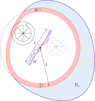
Figure 9: For the proof of Proposition 18.

The connection between border points and the number of crossing edges can be made via Euler’s relation, since it follows that a crossing edge is an edge of the (planar) subgraph of $\operatorname{DT}(\mathbf{\Phi})$ induced by the points which either lie inside $W$, are border points, or lie outside of $W^{\odot}$ and have a neighbour in $W$. Let $B_{W}$ denote of set of border points, $E_{W}$ the collection of crossing edges, and $Y_{W}$ the collection of points lying outside of $W^{\odot}$ and having a Delaunay neighbour within $W$. Then

$$A(z)\leq|E_{W}|\leq 3(|W\cap\mathbf{\Phi}|+|B_{W}|+|Y_{W}|).$$ (15)

Proposition 16 bounds $|W\cap\mathbf{\Phi}|$, as this is exactly the set of visited vertices. Lemmas 19 and 20 bounding $|B_{W}|$ and $|Y_{W}|$ complete the proof. ∎

Lemma 19.

For all $n$ large enough, we have

$$\mathbb{P}\bigg{(}|Y_{W}|\geq 10\max\{L_{0},\omega_{n}^{5}\}\bigg{)}\leq 2\exp\left(-\omega_{n}^{5/4}\right).$$

Proof.

Heuristically, our proof will follow from the fact that, with high probability, a Delaunay edge away from the boundary of the domain is not long enough to span the distance between a point within the walk, and a point outside of $W^{\odot}$. Unfortunately our proof is complicated by points on the walk which are very close to the boundary of the domain, since in this case, those points might have ‘bad’ edges which are long enough to escape $W^{\odot}$. To deal with this, we will take all points in the walk that are close to the border, and imagine that every Delaunay edge touching one of these points is such a ‘bad’ edge. The total number of these edges will be bounded by the maximum degree.

To begin, we give the first case. Consider an arbitrary point $x\in W\cap\mathbf{\Phi}$ that is at least $\omega_{n}^{-3}$ away from the boundary of $\mathcal{D}_{n}$. Suppose this point has a neighbour outside of $W^{\odot}$, then its circumcircle implicitly overlaps an unconditioned region of $\mathcal{D}_{n}$ with area at least $c\,\omega_{n}^{-3}\,\omega_{n}^{5}=c\,\omega_{n}^{2}$ (for $c>0$ a constant depending on the shape of the domain). The probability that this happens for $x$ is thus at most $\exp\left(-\omega_{n}^{2}\right)$. Now note that there are at most $2n$ points in $\mathbf{\Phi}$ with probability bounded by $\exp\left(-\omega_{n}^{2}\right)$ and at most $4n^{2}$ edges between points of $x\in W\cap\mathbf{\Phi}$ and $x\in\{W^{\odot}\}^{c}\cap\mathbf{\Phi}$. By the union bound, the probability that any such edge exists is at most

$$(4n^{2})\exp\left(-c\,\omega_{n}^{2}\right)+\exp\left(-\omega_{n}^{2}\right)\leq\exp\left(-\omega_{n}^{3/2}\right).$$

For the second case, we count the number of points within $\omega_{n}^{-3}$ of the boundary of the domain. Using standard arguments, we have that there are no more than $10\max\{L,\omega_{n}^{5}\}\cdot\omega_{n}^{-3}$ such points, with probability at least $\exp\left(-\omega_{n}^{2}\right)$. Each of these has at most $\Delta_{\mathbf{\Phi}}$ edges that could exit $W^{\odot}$, where $\Delta_{\mathbf{\Phi}}$ is the maximum degree of any vertex in $\operatorname{DT}(\mathbf{\Phi})$, which is bounded in Proposition 30. Thus, the number of such bad edges is at most $10\max\{L,\omega_{n}^{5}\}\omega_{n}^{-3}\cdot\omega_{n}^{3}$ with probability at least $\exp(-\omega_{n}^{2})+\exp(-\omega_{n}^{5/4})$ ∎

Lemma 20.

For all $n$ large enough, and universal constant $C>0$,

$$\mathbb{P}\bigg{(}|B_{W}|\geq C\max\{L_{0},\omega_{n}^{6}\}\bigg{)}\leq 2\exp\left(-\omega_{n}^{3/2}\right).$$

Proof.

Since $|B_{W}|$ is a sum of indicator random variables, it can be bounded using (a version of) Chernoff–Hoeffding’s method. The only slight annoyance is that the indicators $\mathbf{1}_{\{x\in B_{W}\}},x\in\mathbf{\Phi}\cap W^{\odot}$ are not independent. Note however that $\mathbf{1}_{\{x\in B_{W}\}}$ and $\mathbf{1}_{\{y\in B_{W}\}}$ are only dependent if the discs used to define membership to $B_{W}$ for $x$ and $y$ intersect. There is a priori no bound on the radius of these discs, and so we shall first discard the points $x\in\mathbf{\Phi}$ lying far away from $\partial W^{\odot}$ and $W$. More precisely, let $B_{W}^{\star}$ denote the set of border points lying within distance $\omega_{n}$ of either $W$ or $\partial W^{\odot}$, and $B_{W}^{\bullet}=B_{W}\setminus B_{W}^{\star}$. Observe now that we may bound $|B_{W}^{\bullet}|$ directly using Lemma 10, since a point is only a border point if one of its cones is empty, and each such empty cone contains a large empty circle. So for sufficiently large $n$,

$$\mathbb{P}\big{(}|B_{W}^{\bullet}|\neq 0\big{)}\leq\exp\left(-\omega_{n}^{3/2}\right).$$ (16)

Bounding $|B_{W}^{\star}|$ is now easy since the amount of dependence in the family $\mathbf{1}_{\{x\in B_{W}\}},x\in\mathbf{\Phi}\setminus W$ is controlled and we can use the inequality by Janson [16, 15]. We start by bounding the expected value $\mathbb{E}\,|B_{W}^{\star}|$. Note that for a single point $x\in\mathbf{\Phi}_{n}$, by definition the disc used to define whether $x$ is a border point does not intersect $W$ and stays entirely within $\mathcal{D}$, so

$$\mathbb{P}_{x}(x\in B_{W}^{\star})=\mathbb{P}(x\in B_{W}^{\star}) \leq 24\exp\left(-\frac{\pi}{32}\min\{\|xW\|,\|x\partial W^{\odot}\|\}^{2}\right)$$

$$\leq 24\exp\left(-\frac{\pi}{32}\|xW\|^{2}\right)+24\exp\left(-\frac{\pi}{32}\|x\partial W^{\odot}\|^{2}\right)$$ (17)

and $\mathbf{\Phi}_{n}$ is unconditioned in $\mathcal{D}\setminus W$. Partition $\mathcal{D}\setminus W$ into disjoint sets as follows:

$$\mathcal{D}\setminus W=\bigcup_{i=0}^{\infty}U_{i}$$

where $U_{i}:=\{x\in\mathcal{D}\;:\;i\leq\|xW\|<i+1\}.$ Similarly, the sets $U_{i}^{\prime}:=\{x\in W^{\odot}:i\leq\|x\partial W^{\odot}\|<i+1\}$ form a similar partition for $W^{\odot}$. Writing $\lambda$ for the 2-dimensional Lebesgue measure and using (3.3) above, we have

$$\mathbb{E}|B_{W}^{\star}| =\mathbb{E}\left[\sum_{x\in\mathbf{\Phi}}\mathbf{1}_{\{x\in W^{\odot}\setminus W\}}\;\mathbf{1}_{\{x\in B^{\star}_{W}\}}\right]$$

$$=\int_{W^{\odot}\setminus W}\mathbb{P}_{x}(x\in B^{\star}_{W})\,\lambda(dx)$$

$$\leq\sum_{i=0}^{\infty}\int_{U_{i}}24\exp\left(-\pi i^{2}/32\right)\,\lambda(dx)+\sum_{i=0}^{\infty}\int_{U_{i}^{\prime}}24\exp\left(-\pi i^{2}/32\right)\,\lambda(dx)$$

$$=24\sum_{i=0}^{\infty}(\lambda(U_{i})+\lambda(U_{i}^{\prime}))\;\exp\left(-\pi i^{2}/32\right).$$

We may now bound $\lambda(U_{i})$ and $\lambda(U_{i}^{\prime})$ as follows. Recall that $W$ is a union of discs $W=\cup_{i}D_{i}$. We clearly have that

$$U_{i} \subseteq\bigcup_{j=0}^{\kappa-1}\big{\{}x\in\mathcal{D}\;:\;i\leq\|xD_{j}\|<i+1\big{\}}.$$

Note that

$$\lambda\big{(}\big{\{}x\in\mathcal{D}\;:\;i\leq\|xD_{j}\|<i+1\big{\}}\big{)} \leq\pi((R_{j}+i+1)^{2}-(R_{j}+i)^{2})$$ (18)

$$=\pi(2(R_{j}+i)+1).$$ (19)

So, assuming there are $\kappa$ steps in the walk we get

$$\lambda(U_{i}) \leq\sum_{j=0}^{\kappa-1}\pi(2(R_{j}+i)+1)=2\pi\sum_{j=0}^{\kappa-1}R_{j}+\pi(i+1)\kappa.$$

Regarding $\lambda(U_{i}^{\prime})$, note first that $W^{\odot}$ is convex for it is the intersection of two convex regions. It follows that its perimeter is bounded by $4\pi\max\{\|zq\|,\omega_{n}\}$, so that $\lambda(U_{i}^{\prime})\leq 4\pi\max\{\|zq\|,\omega_{n}\}$ for every $i\geq 0$. It now follows easily that there exist universal constants $C,C^{\prime}$ such that

$$\mathbb{E}\,|B^{\star}_{W}|=\mathbb{E}\,\mathbb{E}\big{[}|B_{W}^{\star}|\;\big{|}\;R_{i},i\geq 0\big{]} \leq C\,\mathbb{E}\left[\sum_{j=0}^{\kappa-1}R_{j}+\kappa+\max\{\|zq\|,\omega_{n}\}\right]$$

$$\leq C^{\prime}\max\{\|zq\|,\omega_{n}\}.$$

For the concentration, we use the fact that if $\|xW\|,\|x\partial W^{\odot}\|\leq\omega_{n}$ then the chromatic number $\chi$ of the dependence graph of the family $\mathbf{1}_{\{x\in B^{\star}_{W}\}}$ is bounded by the maximum number of points of $\mathbf{\Phi}_{n}$ contained in a disc of radius $2\omega_{n}$. We then have

$$\mathbb{P}(\chi\geq 8\pi\omega_{n}^{2}) \leq\mathbb{P}(\exists x\in\mathcal{D}:\mathbf{\Phi}_{n}\cap b(x,2\omega_{n}))$$

$$\leq\mathbb{E}\left[\sum_{x\in\mathbf{\Phi}_{n}}\mathbb{P}_{x}(|b(x,2\omega_{n})\cap\mathbf{\Phi}_{n}|\geq 8\pi\omega_{n}^{2})\right]$$

$$\leq\mathbb{E}\left[\sum_{x\in\mathbf{\Phi}_{n}}\mathbb{P}(\operatorname{Po}(4\pi\omega_{n}^{2})\geq 8\pi\omega_{n}^{2})\right]$$

$$\leq\exp\left(-\omega_{n}^{2}\right),$$

for all $n$ large enough, using the bounds for Poisson random variables we have already used in the proof of Corollary 15. Let

$$W^{\partial}:=\big{\{}x\in W^{\odot}\;\big{|}\;\max\{\|xW\|,\|x\partial W^{\odot}\|\}\leq\omega_{n}\big{\}}.$$

Following Equation (18) and by the convexity of $W^{\odot}$, there exists a universal constant $C^{\prime\prime}$ such that

$$\mathbb{P}\bigg{(}|\mathbf{\Phi}_{n}\cap W^{\partial}|\geq C^{\prime\prime}\max\{L,\omega_{n}^{5}\}\cdot\omega_{n}^{2}\Bigg{)}\leq\exp\left(-\omega_{n}^{2}\right).$$

By Theorem 3.2 of [15], we thus obtain for $t>0$,

$$\mathbb{P}(|B^{\star}_{W}|\geq\mathbb{E}\,|B^{\star}_{W}|+t)$$

$$\leq\mathbb{E}\left[\exp\left(-\frac{2t^{2}}{\chi\cdot|\mathbf{\Phi}_{n}\cap W^{\partial}|}\right)\right]$$

$$\leq\exp\left(-\frac{t^{2}}{8\pi\,C^{\prime\prime}\max\{L_{0},\omega^{5}_{n}\}\cdot\omega_{n}^{4}}\right)+\mathbb{P}\Big{(}\chi\geq 8\pi\omega_{n}^{2}\Big{)}+\mathbb{P}\Big{(}|\mathbf{\Phi}_{n}\cap W^{\partial}|>C^{\prime\prime}\max\{L_{0},\omega^{5}_{n}\}\cdot\omega_{n}^{2}\Big{)}$$

$$\leq\exp\left(-\frac{t^{2}}{8\pi\,C^{\prime\prime}\max\{L_{0},\omega^{5}_{n}\}\cdot\omega_{n}^{4}}\right)+2\exp\left(-\omega_{n}^{2}\right).$$

The result follows for $n$ sufficiently large by choosing $t:=C^{\prime\prime}\left(L_{0}+\omega^{6}_{n}\right)$. ∎

3.4 Algorithmic complexity

Whilst we have given explicit bounds on the number of sites in $\mathbf{\Phi}_{n}$ that may be accessed by an instance of Cone-Walk, we recall that the complexity of the algorithm $\textnormal{Cone-Walk}(z,q)$ does not follow directly. This is because the Cone-Walk algorithm must do a small amount of computation at each step in order to compute the vertex which should be chosen next. We proceed by defining a random variable $T(z,q)$, which will denote the number of operations required by $\textnormal{Cone-Walk}(z,q)$ in the RAM model of computation given an implementation based upon a priority queue. We conjecture that the bound for Proposition 21 given in this section is not tight, and that the algorithmic complexity is fact be bounded by $O(L_{0}+\omega_{n}^{4})$. Unfortunately the dependency structure in algorithms of this type makes such bounds difficult to attain.

Proposition 21.

Let $T(z,q)$ be the number of steps required by the Cone-Walk algorithm to compute the sequence of stoppers given by the cone-walk process between $z$ and $q$ along with the path generated by Simple-Path in the RAM model of computation. Let $c_{1}>0$ be an implementation-dependent constant, then for $n$ large enough, we have

$$\mathbb{P}\bigg{(}T(z,q)>c_{1}\cdot L_{0}\log\omega_{n}+\omega_{n}^{4}\bigg{)}\leq 10\exp\left(-\omega_{n}^{3/2}\right).$$

Proof.

Define $M_{i}$ to be the number of sites accessed during the $i$’th step of the algorithm. We fix $z,q$ and write $T$ to denote $T(z,q)$ for brevity. From Section 2.3, we know that for sufficiently large $n$, we may choose a constant $c_{2}$ such that

$$T\leq c_{2}\sum_{i=0}^{\kappa-1}\tau_{i}\log(M_{i}).$$ (20)

So that to bound $T$, it suffices to bound the sum in (20). We have

$$\begin{split}\mathbb{P}\bigg{(}\sum_{i=0}^{\kappa-1}\tau_{i}&\log(M_{i})\geq 15(L_{0}+{\omega_{n}}^{3})\log(\omega_{n})\bigg{)}\\ &\leq\mathbb{P}\bigg{(}\sum_{i=0}^{\kappa-1}\tau_{i}\log(M_{i})\geq 3(L_{0}+{\omega_{n}}^{3})\log(\omega_{n}^{5})\mid M_{\text{max}}<\omega_{n}^{5}\bigg{)}+\mathbb{P}\bigg{(}M_{\text{max}}\geq\omega_{n}^{5}\bigg{)}\\ &\leq\mathbb{P}\bigg{(}\sum_{i=0}^{\kappa-1}\tau_{i}\geq 3(L_{0}+{\omega_{n}}^{3})\bigg{)}+\exp\left(-\omega_{n}^{3/2}\right).\end{split}$$

The first term of which is bounded by Proposition 16, and the bound on $M_{\text{max}}$ comes directly from the proof of Proposition 11. ∎

4 Relaxing the model and bounding the cost of the worst query

4.1 About the shape of the domain and the location of the aim

The analysis in Section 3 was provided given the assumption that $q$ was the centre of a disc containing $\mathbf{\Phi}$ for clarity of exposition. We now relax the assumptions on both the shape of the domain $\mathcal{D}$ and the location of the query $q$. Taking $\mathcal{D}$ to be a disc with $q$ at its centre ensured that $\operatorname{Disc}(z,q,r)$ was included in $\mathcal{D}$ for $r\leq\|zq\|$ and thus the search cone and disc were always entirely contained in the domain $\mathcal{D}$. If we now allow $q$ to be close to the boundary, it may be that part of the search cone goes outside $\mathcal{D}$.

To begin with, we leave $\mathcal{D}$ unchanged and allow $q$ to be any point in $\mathcal{D}$. Given any point $z\in\mathcal{D}$, the convexity of $\mathcal{D}$ ensures that the line segment $zq$ lies within $\mathcal{D}$. Furthermore, one of the two halves of the disc of diameter $zq$ is included within $\mathcal{D}$. Thus for any $z,q\in\mathcal{D}$ and $r\in\mathbb{R}$ the portion of $\operatorname{Cone}(z,q,r)$ (resp. $\operatorname{Disc}(z,q,r)$) within $\mathcal{D}$ has an area lower bounded by half of its actual area (including the portion outside $\mathcal{D}$). Since the distributions of all of the random variables rely on estimations for the portions of area of $\operatorname{Cone}(z,q,r)$ or $\operatorname{Disc}(z,q,r)$ lying inside $\mathcal{D}$, we have the same order of magnitude for $\kappa$, $K$, $\Lambda$ and $T$, with only a degradation of the relevant constants. The proofs generalise easily, and we omit the details. (Note however, that upper and lower bounds in an equivalent of Proposition 14 would not match any longer.)

The essential property we used above is that a disc with a diameter within $\mathcal{D}$ has one of its halves within $\mathcal{D}$. This is still satisfied for smooth convex domains $\mathcal{D}$ and for discs whose radius is smaller than the minimal radius of curvature of $\partial\mathcal{D}$. Thus our analysis may be carried out provided all the cones and discs we consider are small enough. The conditioning on the event $G_{k}$ which we used in Section 3 precisely guarantees that for all $n$ large enough, on $G_{k}$, all the regions we consider are small enough ($O(\log n/\sqrt{n}\,)=o(1)$ in this scaling), and that $G_{k}$ still occurs with high probability. These remarks yield the following result. As before, $\mathcal{D}_{n}=\sqrt{n}\mathcal{D}$ denotes the scaling of $\mathcal{D}$ with area $n$.

Proposition 22.

Let $\mathcal{D}$ be a fixed smooth convex domain of area $1$ and diameter $\delta$. Consider a Poisson point process $\mathbf{\Phi}_{z}^{n}$ of intensity $1$ contained in $\mathcal{D}_{n}=\sqrt{n}\mathcal{D}$. Let $z,q\in\mathcal{D}_{n}$. Let $\mathbf{\Phi}_{z}^{n}$ be $\mathbf{\Phi}^{n}$ conditioned on $z\in\mathbf{\Phi}^{n}$. Then, there exist constants $C_{\Gamma,\mathcal{D}}$, $A_{\Gamma,\mathcal{D}}$, $\Gamma\in\{\kappa,K,\Lambda,T\}$, such that for the cone walk on $\mathbf{\Phi}_{z}^{n}$, and all $n$ large enough, we have

$$\sup_{z,q\in\mathcal{D}_{n}}\mathbb{P}\left(\Gamma(z,q)>C_{\Gamma,\mathcal{D}}\cdot\|zq\|+(1+\sqrt{\|zq\|})\omega_{n}^{5}\,\right)\leq A_{\Gamma,\mathcal{D}}\cdot\exp\left(-\omega_{n}^{3/2}\right).$$

Thus we obtain upper tail bounds for the number of steps $\kappa(z,q)$, the number of visited sites $K(z,q)$, the length $\Lambda(z,q)$ and the complexity $T(z,q)$ which are uniform in the starting point $z$ and the location of the query $q$. We now move on to strengthening the results to the worst queries (still in a random Delaunay).

4.2 The worst query in a Poisson Delaunay triangulation

In this section, we prove a Poissonised version of Theorems 1 and 3. The proof of the latter are completed in Section 4.3. Consider $\sup_{z\in\mathbf{\Phi}^{n},q\in\mathcal{D}_{n}}\Gamma(z,q)$, the value of the parameter for the worst possible pair of starting point and query location, for $\Gamma\in\{\kappa,K,\Lambda,T\}$.

Theorem 23.

There exist a constant $C_{\Gamma,\mathcal{D}}$ depending only on $\Gamma$ and on the shape of $\mathcal{D}$ such that, for all $n$ large enough,

$$\mathbb{P}\bigg{(}\exists z\in\mathbf{\Phi}^{n},\,q\in\mathcal{D}_{n}~{}:~{}\Gamma(z,q)>C_{\Gamma,\mathcal{D}}\cdot\|zq\|+(1+\sqrt{\|zq\|})\log^{4}n\,\bigg{)} \leq\frac{1}{n^{2}}.$$

By Lemma 9, the number of possible walks in a given Delaunay tessellation of size $n$ is at most $n\times n^{4}$. Although it seems intuitively clear that this should be sufficient to bound the parameters for the worst query, it is not the case: one needs to guarantee that there is a way to sample points independently from $\mathbf{\Phi}^{n}$ such that all the cells are hit, or in other words that the cells are not too small. We prove the following:

Proposition 24 (Stability of the walk).

There exists a partition of $\mathcal{D}$ into at most $2n^{4}$ cells such that the sequence of steps used by the cone walk algorithm from any vertex of the triangulation does not change when $q$ moves in a region of the partition. Furthermore, let $a(\mathbf{\Phi}^{n})$ denote the area of the smallest cell. Then

$$\mathbb{P}(a(\mathbf{\Phi}^{n})<\eta)<1-O(n^{8}\eta^{1/3}),$$

for all $n$ large enough.

The proof of Proposition 24 relies on bounds on the smallest angle and on the shortest line segment in the line arrangement. The argument is rather long, and we think it would dilute too much the focus of this section, so we prove it in Section 5.

Proof of Theorem 23.

In order to control the behaviour of the walk aiming at any point $q\in\mathcal{D}$, it suffices to control it for one point of each face of the subdivision associated with the line arrangement $\Xi(\mathbf{\Phi}^{n})$ introduced in Section 2.4. Let $\mathcal{Q}_{n}=\{q_{i}:1\leq 1\leq n^{2k})\}$, for some $k\geq 1$ to be chosen later, be a collection of i.i.d. uniform random points in $\mathcal{D}$, independent of $\mathbf{\Phi}^{n}$. Let $E_{n}$ be the event that every single face of the subdivision contains at least one point of $\mathcal{Q}_{n}$. Since there are at most $|\mathbf{\Phi}^{n}|^{4}$ regions, Proposition 24 implies that

$$\mathbb{P}(E_{n}^{c}) \leq\mathbb{P}\big{(}E_{n}^{c}~{}|~{}a(\mathbf{\Phi}^{n})\geq n^{-k}\big{)}+\mathbb{P}\big{(}a(\mathbf{\Phi}^{n})<n^{-k}\big{)}$$

$$\leq\mathbb{E}[|\mathbf{\Phi}^{n}|^{4}]\cdot\mathbb{P}(\text{Bin}(n^{2k},n^{-k})=0)+O(n^{8}\cdot n^{-k/3})$$

$$=O(n^{4}\cdot\exp\left(-n^{k/2})\right)+O(n^{8-k/3})$$

$$=O(n^{8-k/3}).$$ (21)

For $x>0$ write $f_{n}(x):=C_{\Gamma,\mathcal{D}}x+(1+\sqrt{x})\log^{4}n$. Then, we have

$$\mathbb{P}\big{(}\exists z\in\mathbf{\Phi}^{n},q\in\mathcal{D}_{n}~{}:~{}\Gamma(z,q)\geq f_{n}(\|zq\|)\big{)}$$

$$\leq\mathbb{P}\big{(}\exists z\in\mathbf{\Phi}^{n},q\in\mathcal{D}_{n}~{}:~{}\Gamma(z,q)\geq f_{n}(\|zq\|)~{}\big{|}~{}E_{n}\big{)}+\mathbb{P}(E_{n}^{c})$$

$$=\mathbb{P}\big{(}\exists z\in\mathbf{\Phi}^{n},q\in\mathcal{Q}_{n}~{}:~{}\Gamma(z,q)\geq f_{n}(\|zq\|)\big{)}+\mathbb{P}(E_{n}^{c})$$

$$\leq n^{2k}\cdot\sup_{q\in\mathcal{D}}\mathbb{P}\big{(}\exists z\in\mathbf{\Phi}^{n}~{}:~{}\Gamma(z,q)\geq f_{n}(\|zq\|)\big{)}+\mathbb{P}(E_{n}^{c}).$$ (22)

Now for any fixed $q\in\mathcal{D}$, and conditioning on $\mathbf{\Phi}^{n}$, we see that

$$\mathbb{P}\big{(}\exists z\in\mathbf{\Phi}^{n}~{}:~{}\Gamma(z,q)\geq f_{n}(\|zq\|)\big{)} \leq\mathbb{E}\bigg{[}\sum_{z\in\mathbf{\Phi}^{n}}\mathbf{1}_{\{\Gamma(z,q)\geq f_{n}(\|zq\|)\}}\bigg{]}$$

$$\leq\mathbb{E}\bigg{[}\sum_{z\in\mathbf{\Phi}^{n}}\mathbf{1}_{\{\Gamma(z,q)\geq f_{n}(\|zq\|),|\mathbf{\Phi}^{n}|\leq 2n\}}\bigg{]}+\mathbb{P}\left(|\mathbf{\Phi}^{n}|>2n\right)$$

$$\leq 2n\sup_{z\in\mathcal{D}}\mathbb{P}(\Gamma(z,q)\geq f_{n}(\|zq\|))+\exp\left(-n/3\right).$$

The claim follows from (4.2), (4.2), and Proposition 22 by choosing $k=40$. (Note that we could easily obtain sub-polynomial bounds.) ∎

Before concluding this section, we note that the same arguments also yield the Poissonised version of Theorem 1 about the number of neighbourhoods required to compute all the steps of any query. We omit the proof.

Theorem 25.

We have the following bound for any run of Cone-walk on $\operatorname{DT}(\mathbf{\Phi}^{n})$, for $\mathbf{\Phi}^{n}$ a Poisson point process of rate $n$ in $\mathcal{D}$:

$$\mathbb{P}\Big{(}\exists z\in\mathbf{\Phi}^{n},q\in\mathcal{D}_{n}:M(z,q)>\log^{1+\epsilon}n\Big{)}\leq\frac{1}{n^{2}}.$$

4.3 De-Poissonisation: Proof of Theorem 3

In this section, we prove that the results proved in the case of a Poisson point process of intensity $n$ in a compact convex domain $\mathcal{D}$ (Theorem 23) may be transferred to the situation where the collection of sites consists of $n$ independent uniformly random points in $\mathcal{D}$. In the present case, the concentration for our events is so strong that the de-Poissonisation is straightforward.

Note that conditional on $|\mathbf{\Phi}^{n}|=n$, the collection of points $\mathbf{\Phi}^{n}$ is precisely distributed like $n$ independent uniforms in $\mathcal{D}$. Furthermore, $|\mathbf{\Phi}^{n}|$ is a Poisson random variable with mean $n$, so that by Stirling’s formula, as $n\to\infty$,

$$\mathbb{P}(|\mathbf{\Phi}^{n}|=n)=\frac{n^{n}\exp\left(-n\right)}{n!}\sim\frac{1}{\sqrt{2\pi n}}.$$ (23)

This is small, but we can consider multiple copies of the process; if one happens to have exactly $n$ points, but that none of them actually behaves badly, then it must be the case that the copy that has $n$ points behave as it should, which is precisely what we want to prove. To make this formal, consider a sequence $\mathbf{\Phi}^{n}_{i}$, $i\geq 1$, of i.i.d. Poisson point processes with mean $n$ in $\mathcal{D}$. Let $\eta_{n}$ be the first $i\geq 1$ for which $|\mathbf{\Phi}^{n}_{i}|=n$. Then, for any event $E^{i}$ defined on $\mathbf{\Phi}^{n}_{i}$,

$$\mathbb{P}(E_{1}\,|\,|\mathbf{\Phi}^{n}_{1}|=n) =\mathbb{P}(E_{\eta_{n}})$$

$$\leq\mathbb{P}(\exists j\leq\eta_{n}:E_{j})$$

$$\leq\mathbb{P}(\exists j\leq n:E_{j},\eta_{n}\leq n)$$

$$\leq n\mathbb{P}(E_{1})+\mathbb{P}(\eta_{n}\geq n)$$

$$\leq n\mathbb{P}(E_{1})+\exp\left(-\sqrt{n/(2\pi)}\right),$$

where the last line follows from (23). In the present case, we apply the argument above to estimate the probabilities that the number of steps, the number of sites visited, the length of the walk or the complexity of the algorithm exceeds a certain value. In the case of the Poisson point process, we have proved that any of these events has probability at most $1/n^{2}$, so that we immediately obtain a bound of $O(1/n)$ in the case of $n$ i.i.d. uniformly random points, which proves the main statement in Theorem 3.

This implies immediately that, for $\delta$ the diameter of $\mathcal{D}$, we have

$$\mathbb{E}\bigg{[}\sup_{z\in\mathbf{X}^{n},q\in\mathcal{D}_{n}}\Gamma(z,q)\bigg{]} \leq 2\delta C_{\Gamma}\sqrt{n}+\mathbb{P}\bigg{(}\sup_{z\in\mathbf{X}_{n},q\in\mathcal{D}_{n}}\Gamma(z,q)\geq 2\delta C_{\Gamma}\sqrt{n}\bigg{)}$$

$$\leq 2\delta C_{\Gamma}\sqrt{n}+O(1/n)$$

$$\leq 3\delta C_{\Gamma}\sqrt{n},$$

for $n$ large enough, so that the proof of Theorem 3 is complete. The proof of Theorem 1 from Theorem 25 relies on the same ideas and we omit the proof.

5 Extremes in the arrangement $\Xi(\mathbf{\Phi}^{n})$

In this section, we obtain the necessary results about the geometry of the line arrangement $\Xi$ introduced in Section 2.4.4. In particular, we prove Proposition 24 providing a uniform lower bound on the areas of the cells of the subdivision associated to $\Xi$ which is crucial to the proofs of our main results Theorems 1 and 3.

The rays (half-lines) of the arrangement $\Xi$ all have one end at a site of $\mathbf{\Phi}^{n}$. Let $\Xi_{x}$ denotes the set of rays of $\Xi$ with one end at $x$; we say that the rays in $\Xi_{x}$ originate at $x$. The rays come in two kinds:

• regular rays are defined by a triple $x,y,y^{\prime}$ such that there exists $r>0$ and $q\in\mathbb{R}^{2}$ for which $y$ and $y^{\prime}$ both lie on the front arc of the $\operatorname{Cone}(x,q,r)$; such a ray is denoted by $\rho^{-}(x,y,y^{\prime})$;

• extreme rays correspond to one of the straight boundaries of $\operatorname{Cone}(x,y,\infty)$, for some pair of points $x$, $y$; these two rays are denoted by $\rho^{+}_{1}(x,y)$ and $\rho^{+}_{2}(x,y)$ in such a way that the angle from $\rho^{+}_{1}$ to $\rho^{+}_{2}$ is $\pi/4$.

We let $\Xi_{x}^{-}$ and $\Xi_{x}^{+}$ denote the collections of regular and extreme rays of $\Xi_{x}$, respectively. Our strategy to bound the area of the smallest cell is to lower bound the angle between any two rays (Section 5.1) and the length of any line segment (Section 5.2). We put together the arguments and prove Proposition 24 in Section 5.3.

5.1 The smallest angle between two rays

We start with a bound on the smallest angle in the arrangement.

Lemma 26.

Let $\langle\mathbf{\Phi}^{n}\rangle$ denote the minimum angle between any two lines of $\Xi(\mathbf{\Phi}^{n})$ which intersect within $\mathcal{D}$. Then, there exists a constant $C$ such that, for any $\beta\in(0,\pi/8)$,

$$\mathbb{P}(\langle\mathbf{\Phi}^{n}\rangle<\beta)\leq Cn^{5}\beta.$$

Proof.

For two intersecting rays $\rho_{1}$ and $\rho_{2}$, let $\langle\rho_{1},\rho_{2}\rangle$ denote the (smallest) angle they define. We first deal with the angles between two rays originating from different points. Consider a given ray $\rho_{1}\in\Xi_{x_{1}}$, and let $\tilde{x}_{1}$ denote the intersection of $\rho_{1}$ with $\partial\mathcal{D}$. For another ray $\rho_{2}\in\Xi_{x_{2}}$, with $x_{2}\neq x_{1}$, to intersect $\rho_{1}$ at an angle lying in $(-\beta,\beta)$, we must have $x_{2}\in\operatorname{Cone}_{\beta}(x_{1},\tilde{x}_{1},\infty)\cup\operatorname{Cone}_{\beta}(\tilde{x}_{1},x_{1},\infty)$. Observe that for any two points $x,y$, the area of $\operatorname{Cone}_{\beta}(x,y,\infty)\cap\mathcal{D}$ is bounded by $\delta^{2}\tan\beta$, where $\delta$ denotes the diameter of $\mathcal{D}$. In particular, for any fixed ray $\rho_{1}\in\Xi_{x}$ for some $x\in\mathbf{\Phi}^{n}$,

$$\mathbb{P}(\exists x_{2}\in\mathbf{\Phi}^{n}_{x}\setminus\{x\},\rho_{2}\in\Xi_{x_{2}}:\langle\rho_{1},\rho_{2}\rangle<\beta)$$

$$\leq\mathbb{P}(\exists x_{2}\in\mathbf{\Phi}^{n}_{x}\setminus\{x\}:x_{2}\in\operatorname{Cone}_{\beta}(x_{1},\tilde{x}_{1},\infty))$$

$$\quad+\mathbb{P}(\exists x_{2}\in\mathbf{\Phi}^{n}_{x}\setminus\{x\}:x_{2}\in\operatorname{Cone}_{\beta}(\tilde{x}_{1},x_{1},\infty))$$

$$\leq 2n\delta^{2}\tan\beta,$$

since $\mathbf{\Phi}_{x}^{n}\setminus\{x\}$ is a Poisson point process in $\mathcal{D}$ with intensity $n$. Now, since for any $x$, $|\Xi_{x}|\leq 2(|\mathbf{\Phi}^{n}|-1)$,

$$\mathbb{P}(\exists x_{1},x_{2}\in\mathbf{\Phi}^{n},x_{1}\neq x_{2},\rho_{1}\in\Xi_{x_{1}},\rho_{2}\in\Xi_{x_{2}}:\langle\rho_{1},\rho_{2}\rangle<\beta)$$

$$\leq\mathbb{E}\Bigg{[}\sum_{x\in\mathbf{\Phi}^{n}}\mathbb{P}(\exists\rho_{1}\in\Xi_{x},x_{2}\in\mathbf{\Phi}^{n}_{x}\setminus\{x\},\rho_{2}\in\Xi_{x_{2}}:\langle\rho_{1},\rho_{2}\rangle<\beta)\Bigg{]}$$

$$\leq\mathbb{E}\Bigg{[}\sum_{x\in\mathbf{\Phi}^{n}}2(|\mathbf{\Phi}^{n}|-1)\cdot 2n\delta^{2}\tan\beta\Bigg{]}$$

$$=4n^{3}\delta^{2}\tan\beta,$$ (24)

since $\mathbf{\Phi}^{n}_{x}\setminus\{x\}$ is distributed like $\mathbf{\Phi}^{n}$.

We now deal with the smallest angle between any two rays in the same set $\Xi_{x}$, for some $x\in\mathbf{\Phi}^{n}$. Any point $y\in\mathbf{\Phi}^{n}_{x}\setminus\{x\}$ defines at most two extreme rays in $\Xi_{x}$ which intersect at an angle of $\pi/4$. For any two distinct points $y,y^{\prime}$ to define two extreme rays that intersect at an angle smaller than $\beta>0$, then $y^{\prime}$ must lie in $\operatorname{Cone}_{\beta}(x,y,\infty)$ or one of its two images in the rotations of angle $+\pi/8$ or $-\pi/8$ about $x$. The arguments we have used to obtain (5.1) then imply that

$$\mathbb{P}(\exists x\in\mathbf{\Phi}^{n}:\exists\rho,\rho^{\prime}\in\Xi_{x}^{+},\langle\rho,\rho^{\prime}\rangle<\beta) \leq 3n^{3}\delta^{2}\tan\beta$$

$$\leq 6n^{3}\delta^{2}\beta,$$

for all $\beta\in[0,\pi/4]$, since then $\tan\beta\leq 2\beta$.

We now consider a regular ray $\rho=\rho^{-}(x,y,z)$. Then there exist $q\in\mathbb{R}^{2}$ and $r>0$ such that $\rho$ is the half-line with an end at $x$ and going through $q$, and $x,y,z$ all lie on the same circle $\mathscr{C}$ (more precisely, $y,z$ lie on the intersection of $\mathscr{C}$ with $\operatorname{Cone}(x,q,\infty)$). We first bound the probability that there exists a point $z^{\prime}$ such that the regular ray $\rho^{\prime}=\rho^{-}(x,y,z^{\prime})$ intersects $\rho$ at an angle at most $\beta$, that is $\rho^{\prime}\in\operatorname{Cone}_{\beta}(x,q,\infty)$. We want to bound the area of the region

$$\{z^{\prime}\in\mathcal{D}:\rho^{-}(x,y,z^{\prime})\in\operatorname{Cone}_{\beta}(x,q,\infty)\},$$

for which the angle between $\rho$ and $\rho^{\prime}$ is at most $\beta$. By definition of $\rho^{\prime}$, $x,y$ and $z^{\prime}$ lie on the same circle $\mathscr{C}^{\prime}=\mathscr{C}^{\prime}(c)$, which has a centre $c^{\prime}$ in $\operatorname{Cone}_{\beta}(x,q,\infty)$. More precisely, the centre $c^{\prime}$ lies on the intersection of the bisector of the line segment $[x,y]$ with $\operatorname{Cone}_{\beta}(x,q,\infty)$; so $c^{\prime}$ lies in a line segment $\ell$ of length $O(\beta)$ containing the centre $c$ of $\mathscr{C}$. The Hausdorff distance between $\mathscr{C}$ and $\cup_{c^{\prime}\in\ell}\mathscr{C}^{\prime}(c)$ is $O(\beta)$ and it follows that

$$\mathcal{A}\{z^{\prime}\in\mathcal{D}:\rho^{-}(x,y,z^{\prime})\in\operatorname{Cone}_{\beta}(x,q,\infty)\}=O(\beta).$$

A similar argument applies to deal with rays $\rho^{-}(x,y^{\prime},z^{\prime})$ for $y^{\prime},z^{\prime}\in\mathbf{\Phi}^{n}$: once the one of $y^{\prime}$ or $z^{\prime}$ is chosen, the second is forced to lie in a region of area $O(\beta)$. From there, arguments similar to the ones we used in (5.1) yield

$$\mathbb{P}(\exists x\in\mathbf{\Phi}^{n}:\exists\rho,\rho^{\prime}\in\Xi_{x}^{-},\langle\rho,\rho^{\prime}\rangle<\beta)=O(n^{5}\beta).$$ (25)

Finally, we deal with the intersections of a regular and an extreme ray. We $\rho=\rho^{-}(x,y,z)$ and $\rho^{\prime}=\rho^{+}_{1}(x,y^{\prime})$, for $y^{\prime}\in\mathbf{\Phi}^{n}$ (potentiall $y^{\prime}=y$). For $\rho^{\prime}$ to lie in $\operatorname{Cone}_{\beta}(x,q,\infty)$, the point $y^{\prime}$ must lie in a cone with apex $x$, half-angle $\beta$ and with axis one of the straight boundaries of $\operatorname{Cone}(x,q,\infty)$. So if $y\neq y^{\prime}$, the point $y^{\prime}$ is constrained to lie in a region of area $O(\beta)$; in this case, the expected number of $x,y,z,y^{\prime}\in\mathbf{\Phi}^{n}$ in such a configuration is $O(n^{4}\beta)$. If on the other hand, $y^{\prime}=y$ then $y$ must lie on a portion of length $O(\beta)$ of the front arc of $\mathscr{C}\cap\operatorname{Cone}(x,q,\infty)$. However, conditional on $x,y,z$ indeed forming the ray $\rho=\rho^{-}(x,y,z)$, the points $y$ is uniformly distributed on the front arc. In other words, the expected number of triplets $x,y,z$ in such a configuration is $O(n^{3}\beta)$. It follows that

$$\mathbb{P}(\exists x\in\mathbf{\Phi}^{n}:\exists\rho\in\Xi_{x}^{-},\rho^{\prime}\in\mathcal{S}_{x}^{+},\langle\rho,\rho^{\prime}\rangle<\beta)=O(n^{4}\beta).$$ (26)

Putting (5.1), (25) and (26) together completes the proof. ∎

5.2 The shortest line segment

Let $L(\mathbf{\Phi}^{n})$ denote the smallest line segment in the arrangement of lines $\Xi(\mathbf{\Phi}^{n})$. The aim of this section is to prove the following:

Lemma 27.

We have, for any $\gamma$ small enough and $n$ large enough,

$$\mathbb{P}(L(\mathbf{\Phi}^{n})<\gamma)\leq n^{9}\gamma^{1/2}.$$

In order to prove Lemma 27, we place a ball of radius $\gamma$ at every intersection in $\Xi(\mathbf{\Phi}^{n})$ (including the ones which involve the boundary $\partial\mathcal{D}$) and estimate the probability that any such ball is hit by another ray of the arrangement. The proof is longer and slightly more delicate than that of Lemma 26 simply because three rays, each involving up to three points of $\mathbf{\Phi}^{n}$, might be involved the event of interest. The first step towards proving Lemma 27 is to establish uniform bounds on the area of location of some points for the rays to intersect a given ball. These bounds are stated in Lemmas 28 and 29 below.

Lemma 28.

There exists a constant $C$ such that, for any $x,y,z\in\mathcal{D}$, one has, for all $\gamma>0$ small enough, we have

1. $\mathcal{A}\{\bar{x}\in\mathcal{D}:\rho^{+}(\bar{x},y)\cap\delta(z,\gamma)\neq\varnothing\}\leq C\gamma$

2. $\mathcal{A}\{\bar{y}\in\mathcal{D}:\rho^{+}(x,\bar{y})\cap\delta(z,\gamma)\neq\varnothing\}\leq C\gamma/\|xz\|.$

Proof.

Fix $x$, $z$ and $\gamma>0$. The location of points $\bar{y}$ for which $\rho^{+}(x,\bar{y})\ni z$ is precisely $\partial\operatorname{Cone}(x,z,\infty)$. Then,

$$\bigcup_{q\in\delta(z,\gamma)}\partial\operatorname{Cone}(x,q,\infty)$$

consists of two cones of half-angle $\arcsin(\gamma/\|xz\|)$, which proves the second claim.

For the first claim, let $c_{1}=c_{1}(z)$ and $c_{2}=c_{2}(z)$ be the two intersections of the circles of radius $\|zy\|/\sqrt{2}$ centred at $y$ and $z$ (so the segment $zy$ is seen from $c_{1}$ and $c_{2}$ at an angle of $\pi/2$). Let $\mathscr{C}_{1}=\mathscr{C}_{1}(z)$ and $\mathscr{C}_{2}=\mathscr{C}_{2}(z)$ denote the discs centred at $c_{1}$ and $c_{2}$, respectively, and having $y$ and $z$ on their boundaries. Then, the region of the points $\bar{x}$ for which $\rho^{+}(\bar{x},y)\ni z$ is precisely the boundary of $\mathscr{C}_{1}\cup\mathscr{C}_{2}$. When looking for the region of points $\bar{x}$ satisfying $\rho^{+}(\bar{x},y)\cap\delta(z,\gamma)\ni q$, for some $q\in\delta(z,\gamma)$ observe that the centres $\|c_{1}(q)-c_{1}(z)\|=O(\gamma)$, $\|c_{2}(q)-c_{2}(z)\|=O(\gamma)$ and that the Hausdorff distance between $\mathscr{C}_{1}(q)\cup\mathscr{C}_{2}(q)$ and $\mathscr{C}_{1}\cup\mathscr{C}_{2}$ is $O(\gamma)$, hence the first claim. ∎

Lemma 29.

There exists a constant $C$ such that, for any $x,y,y^{\prime},z\in\mathcal{D}$, one has, for all $\gamma>0$ small enough

1. $\mathcal{A}\{\bar{x}\in\mathcal{D}:\rho^{-}(\bar{x},y,y^{\prime})\cap\delta(z,\gamma)\neq\varnothing\}\leq C\gamma$

2. $\mathcal{A}\{\bar{y}\in\mathcal{D}:\rho^{-}(x,\bar{y},y^{\prime})\cap\delta(z,\gamma)\neq\varnothing\}\leq C\gamma.$

Proof.

The ray $\rho^{-}(x,y,y^{\prime})$ is the half-line with one end at $x$ and going through the centre $c$ of the circle which contains all three $x,y$ and $y^{\prime}$. So the region of the points $\bar{x}$ for which $\rho^{-}(\bar{x},y,y^{\prime})\ni z$ is naturally indexed by the points of the bisector $\Delta$ of the segment $[y,y^{\prime}]$: for a point $c\in\Delta$, the only possible points $\bar{x}=\bar{x}(c)$ lie the intersection of the circle $\mathscr{C}$ centred at $c$ and containing $y$ (and $y^{\prime}$) and the line containing $c$ and $z$. So if $z\neq c$, there are two such points and at most one of them is such that $y,y^{\prime}\in\operatorname{Cone}(\bar{x},c,\infty)$. If $z=c$, then there is potentially a continuum of points $\bar{x}(c)$, consisting of the arc of $\mathscr{C}$ for which $y,y^{\prime}\in\operatorname{Cone}(\bar{x},c,\infty)$. It follows that for every $c\in\Delta$ such that $\|zc\|>2\gamma$, the points $\bar{x}(c)$ for which $\rho^{-}(\bar{x},y,y^{\prime})$ intersects $\delta(z,\gamma)$ is an arc of length $O(\gamma)$. On the other hand, the cumulated area of the circles $\mathscr{C}(c)$ for which $\|zc\|\leq 2\gamma$ is $O(\gamma)$. Hence the first claim.

For $x$, $y$ and $q$ fixed, the set of points $\bar{y}$ such that $\rho^{-}(x,y,\bar{y})\ni q$ is contained in the circle $\mathscr{C}^{\prime}(q)$ whose centre is the intersection of the bisector of $[x,y]$ and the line $(xq)$, and which contains $x$ (and $y$). The cumulated area of $\mathscr{C}^{\prime}(q)$ when $q\in\delta(z,\gamma)$ is $O(\gamma)$, which proves the second claim. ∎

Proof of Lemma 27.

Recall that, in order to lower bound the length of the shortest line segment in $\Xi(\mathbf{\Phi}^{n})$, we prove using Lemmas 28 and 29, that if we place a ball of radius $\gamma$ at every intersection in $\Xi(\mathbf{\Phi}^{n})$, every ball contains a single intersection with probability at least $1-O(n^{9}\gamma^{1/2})$. The intersections to consider are of three different types: the points $x\in\mathbf{\Phi}^{n}$, the intersections of one ray and the boundary of the domain $\mathcal{D}$, and intersections between two rays.

The case of balls centred at points of $\mathbf{\Phi}^{n}$ first is easily treated. We have

$$\mathbb{P}(\exists z,x\in\mathbf{\Phi}^{n}:z\neq x,\Xi_{x}\cap\delta(z,\gamma)\neq\varnothing) \leq\mathbb{E}\left[\sum_{z\in\mathbf{\Phi}^{n}}\mathbf{1}_{\{\exists x\in\mathbf{\Phi}^{n}\setminus\{z\}:\Xi_{x}\cap\delta(z,\gamma)\neq\varnothing\}}\right].$$

Note that, in the expected value on the right, although $x\neq z$, the set $\Xi_{x}$ does depend on $z$ in a non-trivial way. The main point about the proof is to check that the conditioning on $z\in\mathbf{\Phi}^{n}$ does not make it much easier for a ray to intersect $\delta(z,\gamma)$; and this is where Lemmas 28 and 29 enter the game. We have

$$\mathbb{E}\left[\sum_{z\in\mathbf{\Phi}^{n}}\mathbf{1}_{\{\exists x\in\mathbf{\Phi}^{n}\setminus\{z\}:\Xi_{x}\cap\delta(z,\gamma)\neq\varnothing\}}\right] \leq\mathbb{E}\left[\sum_{z\in\mathbf{\Phi}^{n}}\sum_{y\in\mathbf{\Phi}^{n}}\sum_{x\in\mathbf{\Phi}^{n}\setminus\{z,y\}}\mathbf{1}_{\{\rho^{+}(x,y)\cap\delta(z,\gamma)\neq\varnothing\}}\right]$$

$$+\mathbb{E}\left[\sum_{z\in\mathbf{\Phi}^{n}}\sum_{y,y^{\prime}\in\mathbf{\Phi}^{n}}\sum_{x\in\mathbf{\Phi}^{n}\setminus\{z,y,y^{\prime}\}}\mathbf{1}_{\{\rho^{-}(x,y,y^{\prime})\cap\delta(z,\gamma)\neq\varnothing\}}\right]$$

$$\leq Cn^{4}\gamma,$$

by Lemmas 28 and 29, since conditional on $z,y,y^{\prime}\in\mathbf{\Phi}^{n}$, $\mathbf{\Phi}^{n}\setminus\{x,y,y^{\prime}\}$ is distributed like $\mathbf{\Phi}^{n}$.

We now move on to the intersections of rays with the boundary of $\mathcal{D}$. Let $\rho$ be a ray, and let $z$ denote its intersection with $\partial\mathcal{D}$. If $\rho$ is an extreme ray, then there exists $x,y\in\mathbf{\Phi}^{n}$ such that $\rho=\rho^{+}_{1}(x,y)$ (or $\rho=\rho^{+}_{2}(x,y)$) and we are interested in the probability that some other ray $\rho^{\prime}$ intersects $\delta(z,\gamma)$; note that the ray $\rho^{\prime}$ might arise from a set of points $x^{\prime},y^{\prime}$ (if it is extreme) or $x^{\prime},y^{\prime},y^{\prime\prime}$ (if it is regular) which uses some of $x$ or $y$. If there is at least one point of $x^{\prime},y^{\prime}$ that is not in $\{x,y\}$ then Lemma 28 allows us to bound the probability that $\rho^{+}(x^{\prime},y^{\prime})$ intersects $\delta(z,\gamma)$; in the other case, there must be one of $x^{\prime},y^{\prime},y^{\prime\prime}$ which is not in $\{x,y\}$ and Lemma 29 applies: For each such choice of points, the probability that $\rho^{\prime}$ intersects $\delta(z,\gamma)$ is $O(\gamma)$, uniformly in $x$, $y$ and $z$. So the only case remaining to check is when $\rho^{\prime}$ is only defined by the two points $x,y$. Here,

• either $\rho^{\prime}\in\Xi_{x}$ and for $\rho^{\prime}$ to intersect $\delta(z,\gamma)$ one must have $x\in\delta(z,\gamma)$, which only happens if $x$ lies within distance $\gamma$ of $\partial\mathcal{D}$, hence with probability at most $O(n\gamma)$;

• or $\rho^{\prime}\in\Xi_{y}$ and the ball $\delta(z,\gamma)$ should be close to one of the two points in $\partial\operatorname{Cone}(x,y,\infty)\cap\partial\operatorname{Cone}(y,x,\infty)$; Write $i_{1}=i_{1}(x,y)$ and $i_{2}=i_{2}(x,y)$ for these two points. More precisely, since the angle between $\rho$ and $\rho^{\prime}$ is $\pi/4$, the point $z$ should lie within distance $\gamma\sqrt{2}$ of one of the two intersections (or $\delta(z,\gamma)$ does not intersect $\rho^{\prime}$). Dually, for a point $q$, let $\bar{y}=\bar{y}(q)$ be the point such that $i_{1}(x,\bar{y})=q$. Then, for $\|zq\|\leq\gamma^{\prime}=\gamma\sqrt{2}$ the angle between the vectors $x\bar{y}(q)$ and $x\bar{y}(z)$ is at most $\arcsin(\gamma^{\prime}/\|xz\|)$ and the difference in length is an additive term of at most $\gamma^{\prime}\sqrt{2}$. Overall, $\{\bar{y}:i_{1}(x,\bar{y})\in\delta(z,\gamma^{\prime})\}$ is contained in a ball of radius at most $3\gamma^{\prime}\sqrt{2}=6\gamma$. Finally, since $z\in\partial\mathcal{D}$, the probability that such a situation occurs for some $x,y\in\mathbf{\Phi}^{n}$ is at most $O(n^{2}\gamma)$.

As a consequence, the probability that there exist two rays $\rho$ and $\rho^{\prime}$, such that $\rho^{\prime}\cap\delta(z,\gamma)\neq\varnothing$, for $z=\rho\cap\mathcal{D}$ is $O(n^{5}\gamma)$.

It now remains to deal with the case of balls centred at the intersection of two rays. Consider two rays, $\rho_{1}\in\Xi_{x_{1}}$ and $\rho_{2}\in\Xi_{x_{2}}$, for $x_{1}\neq x_{2}$, which are supposed to intersect at a point $z$ (the case $x_{1}=x_{2}$ has already been covered since then, we have $z\in\mathbf{\Phi}^{n}$). The definition of $\rho_{1}$ and $\rho_{2}$ may involve up to six points $x_{1},y_{1},y_{1}^{\prime}$ and $x_{2},y_{2},y_{2}^{\prime}$ of $\mathbf{\Phi}^{n}$. The probability that some third ray $\rho_{3}$, whose definition uses at least one new point of $\mathbf{\Phi}^{n}$, intersects $\delta(z,\gamma)$ can be upper bounded using Lemmas 28 and 29 as before and we omit the details. The only new cases we need to cover are the ones when the definition of $\rho_{3}$ only involves points among $x_{1},y_{1},y_{1}^{\prime}$ and $x_{2},y_{2},y_{2}^{\prime}$. We now show that all the possible configurations on six points only are unlikely to occur for $\gamma$ small in the random point set $\mathbf{\Phi}^{n}$.

Because of the number of cases to be treated, without a clear way to develop a big picture, we only sketch the remainder of the proof. We treat the cases where $\rho_{1}=\rho^{-}(x_{1},y_{1},y_{1}^{\prime})$ and $\rho_{2}=\rho^{-}(x_{2},y_{2},y_{2}^{\prime})$, so in particular the two rays which intersect at $z$ are regular rays.

• If $\rho_{3}\in\Xi_{x_{1}}$ (or, by symmetry, $\rho_{3}\in\Xi_{x_{2}}$), the bound on the smallest angle between any two rays in Lemma 26 ensures that $z$ ought to be close to $x_{1}$: one must have $\arcsin(\gamma/\|x_{1}z\|)\leq\eta$ where $\eta$ denotes the smallest angle. Then, either $x_{2}$ is also close to $z$, or $y_{2}$ and $y_{2}^{\prime}$ actually almost lie on a circle whose centre lies on the line $(x_{1},x_{2})$. Both are unlikely: (1) the closest pair of points lie at distance $\Omega(1/n)$ (which is much larger than what we are aiming for) and (2) for fixed $x_{1},x_{2}$ and $y_{2}$, the location of points $y_{2}^{\prime}$ such that $y_{2}$ lies near the circle whose centre lies on $(x_{1},x_{2})$ and which contains $y_{2}$ has area of order $O(\gamma)$.

• If $\rho_{3}\in\Xi_{y_{1}}$ (or the other symmetric cases), there are the following possibilities: either $\rho_{3}$ is a regular ray and (up to symmetry)

  $$\rho_{3}\in\left\{\begin{array}[]{l l l l}\text{(a)}&\rho^{-}(y_{1},x_{1},y_{1}^{\prime}),&\text{(b)}&\rho^{-}(y_{1},x_{1},y_{2})\\ \text{(c)}&\rho^{-}(y_{1},x_{2},y_{1}^{\prime}),&\text{(d)}&\rho^{-}(y_{1},x_{2},y_{2})\\ \text{(e)}&\rho^{-}(y_{1},y_{1}^{\prime},y_{2}^{\prime}),&\text{(f)}&\rho^{-}(y_{1},y_{2},y_{2}^{\prime})\end{array}\right\},$$

  or $\rho_{3}$ is an extreme ray and

  $$\rho_{3}\in\big{\{}\begin{array}[]{l l l l}\text{(g)}&\rho^{+}(y_{1},y_{1}^{\prime}),&\text{(h)}&\rho^{+}(y_{1},y_{2})\end{array}\big{\}}.$$

  Since $\rho^{-}(x_{1},y_{1},y_{1}^{\prime})$ is a ray, $y_{1},y_{1}^{\prime}$ both lie in a cone of half-angle $\pi/8$, and it is impossible that we also have $x_{1},y_{1}^{\prime}$ both lying in some cone of half-angle $\pi/8$; so configuration (a) does not occur. For situation (b), we use Lemma 29 (ii). For situations (c)–(f), we use the arguments in the proof of Lemma 29 to exhibit the constraints about the location of the third point defining $\rho_{3}$, once the first two are chosen.

  To deal with the cases where $\rho_{3}\in\Xi_{y_{1}}^{+}$, observe that once $y_{1}$ is placed, $y_{1}^{\prime}$ (or $y_{2}$) must lie in a cone of angle $\arcsin(\gamma/\|y_{1}z\|)$: so either $\|y_{1}z\|\geq r$, and the cone has area $O(\gamma/r)$ or $\|y_{1}z\|\leq r$, but then $y_{1}$ must lie in the portion of the front arc of length $O(r)$ about $\rho_{1}$. Since the conditional distribution of $y_{1}$ is uniform on the arc, the probability that this configuration occurs is $O(\inf_{r\geq 0}\{\gamma/r+r\})=O(\gamma^{1/2})$.

The remaining cases, where at least one of $\rho_{1}$ and $\rho_{2}$ is an extreme ray, may all be treated using similar arguments and we omit the tedious details. ∎

5.3 Lower bounding the area of the smallest cell: Proof of Proposition 24

With Lemmas 26 and 27 under our belt, we are now ready to prove Proposition 24.

We use the line arrangement $\Xi(\mathbf{\Phi}^{n})$ of Section 2.4. The faces of the corresponding subdivision are convex regions delimited by the line segments between intersections of rays, and pieces of the boundary of the domain $\mathcal{D}$. Let $L(\mathbf{\Phi}^{n})$ and $\langle\mathbf{\Phi}^{n}\rangle$ denote the length of the shortest line segment and the smallest angle in the arrangement arising from $\mathbf{\Phi}^{n}$. Consider a face of the subdivision, and one of its vertices $u$ which does not lie on the $\partial\mathcal{D}$. Then the triangle formed by the $u$ and its two adjacent vertices on the boundary of the face is contained in the face. The lengths of the two line segments adjacent to $u$ are at least $L(\mathbf{\Phi}^{n})$ long, and the angle they make lies between $\langle\mathbf{\Phi}^{n}\rangle$ and $\pi-\langle\mathbf{\Phi}^{n}\rangle$, so that the area of the corresponding triangle is at least

$$L(\mathbf{\Phi}^{n})^{2}\cdot\frac{\tan\langle\mathbf{\Phi}^{n}\rangle}{2}.$$

It follows easily from Lemmas 26 and 27 that the area of the smallest face it at least $\beta\gamma/2$ with probability at least $1-O(n^{4}\beta)-O(n^{9}\gamma^{1/2})$. Choosing $\beta,\gamma$ such that $n^{4}\beta=n^{9}\gamma^{1/2}$ yields the claim.

6 Comparison with Simulations

We implemented Cone-Walk in C++ using the CGAL libraries. For simulation purposes, we generated $10^{7}$ points uniformly at random in a disc of area $10^{7}$. We then simulated Cone-Walk on $10^{6}$ different walks starting from a point within a disc having a quarter of the radius of the outer disc (to help reduce border effects) with a uniformly random destination. For comparison, we give give the expected bounds for a walk whose destination is at infinity. See Table 1. With respect to the path, we give two values for the number of extra vertices visited in a step. The first is the number obtained by using Simple-Path and the second, in brackets, is the average number of ‘intermediary vertices’ within each disc.

	Theory	Theory (5 s.f.)	Simulation
Radius	$\mathbb{E}[R]=\sqrt{\frac{\pi}{2\sqrt{2}+\pi}}$	0.72542	0.72557
# Intermediary path steps	$\leq\mathbb{E}[\tau_{i}]\leq\frac{4\pi}{\pi+2\sqrt{2}}$	$\leq$ 1.1049	0.41244 (1.09574)
Simple-Path Length	$\leq\mathbb{E}[\Lambda/L_{0}]\leq\frac{22\pi-4\sqrt{2}}{2+3\pi+8\sqrt{2}}$	$\leq 2.7907$	1.51877

Table 1: Comparison of theory with simulations. Inequalities are used to show when values are bounds.

Appendices

Appendix A Maximum degree for Poisson Delaunay in a smooth convex

Let $\mathbf{\Gamma}$ be a homogeneous Poisson process on the entire Euclidean plane with intensity 1. In this case, Bern et al. [2] give a proof that the expected maximum degree of any vertex of the Delaunay triangulation $\operatorname{DT}(\mathbf{\Gamma})$ falling within the box $[0,\sqrt{n}\,]^{2}$ is $\Theta\left(\frac{\log n}{\log\log n}\right)$. Whilst such a bound may be useful in the analysis of geometric algorithms, it has a shortcoming in that it implicitly avoids dealing with the border effects that occur when considering points distributed within bounded regions. When considering such bounded regions, it can be observed that the degree distribution is significantly skewed near the border, with the majority of the vertices on or near the convex hull having a much higher degree than the global average. It is therefore not altogether trivial that the maximum degree should still be bounded polylogarithmicly when the sites are generated by a homogeneous Poisson process in a bounded region. In this section, we show that this indeed the case for the specific case of a smooth compact convex. As far as we are aware, this is the first such bound that has been given for a set of random points in a bounded region. Let $\mathcal{D}$ be a smooth compact convex subset of $\mathbb{R}^{2}$ with area $\lambda_{2}(\mathcal{D})=1$, and $\mathcal{D}_{n}=\sqrt{n}\mathcal{D}$ (with area $n$ and diameter$(\mathcal{D}_{n})\leq c_{2}\sqrt{n}$, for some constant $c_{2}$). Let $\mathbf{\Phi}$ be a homogeneous Poisson point process of intensity 1 contained within $\mathcal{D}_{n}$, so that in expectation we have $\mathbb{E}\,|\mathbf{\Phi}|=n$. We use $\delta_{\mathbf{\Phi}}(x)$ to denote the degree of $x\in\mathbf{\Phi}$ in $\operatorname{DT}(\mathbf{\Phi})$, and take $\Delta_{\mathbf{\Phi}}:={\displaystyle\max_{x\in\mathbf{\Phi}}\;\delta_{\mathbf{\Phi}}(x)}$.

Proposition 30.

For any $\xi>0$, we have for $n$ sufficiently large,

$$\mathbb{P}\bigg{(}\Delta_{\mathbf{\Phi}}\geq\log^{2+\xi}n\bigg{)}\leq\exp\left(-\log^{1+\xi/4}n\right).$$

Define $\|Ax\|:=\inf\left\{\|xy\|:y\in A\right\}$. Our proof will follow by considering two cases. For the first case we consider all points $x\in\mathbf{\Phi}$ satisfying $\|\partial\mathcal{D}_{n}x\|\leq\sqrt{\log n}$ and bound the number of neighbours of $x$ in $\operatorname{DT}(\mathbf{\Phi})$ to one side of $x$; doubling the result and the end for the final bound. To begin, we trace a ray from $x$ to the point $y\in\partial\mathcal{D}_{n}$ minimising $\|xy\|$; we refer to this as $\mathcal{R}_{0}$. Next, we create a new ray, $\mathcal{R}_{1}$ exiting $x$ such that the area enclosed by $\mathcal{R}_{0}$, $\mathcal{R}_{1}$ and $\partial\mathcal{D}_{n}$ is $\log^{1+\xi}n$; we let $S_{0}$ denote this region. (See Figure 10.) For $n$ large enough, the angle between the rays $\mathcal{R}_{0}$ and $\mathcal{R}_{1}$ is smaller than $\frac{\pi}{2}+\frac{\pi}{12}$. In addition, the length of $\mathcal{R}_{1}$ is upper bounded by the diameter of $\mathcal{D}_{n}\leq c_{2}\sqrt{n}$ and lower bounded by $c_{1}\sqrt{\log n}$ for $c_{1}=\frac{1}{2}$ since $\mathcal{R}_{0}$ is not longer than $\sqrt{\log n}$ by hypothesis.

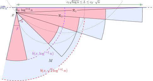
Figure 10: The construction to bound the maximum degree of a vertex near the border. The pink shaded circular sectors are each conditioned to contain at least one point. In this case, no Delaunay neighbour to the right of $x$ can lie outside of the

We then define an iterative process that finishes as soon as one of our regions (that we define shortly) is totally contained within a ball of radius $\log^{1+\xi}n$ about the point $x$. At each step $i$, we look at the ray $\mathcal{R}_{i-1}$ and then grow a sector of a circle with area $\log^{1+\xi}n$, and of radius $\tfrac{1}{\sqrt{2}}|\mathcal{R}_{i-1}|$, where $|\mathcal{R}_{i}|$ is the length of the $i$th ray. The sector of radius $|\mathcal{R}_{i+1}|$ defined by the rays $\mathcal{R}_{i}$ and $\mathcal{R}_{i+1}$ is denoted by $S_{i}$. Thus the internal angle of each new sector is exactly twice that of the previous one. For each sector apart from the first, we add a ‘border’ (shaded blue in Figure 10) which extends the each sector to the length of the sector proceeding it: let $Q_{i}$ be the cone delimited by the rays $\mathcal{R}_{i}$ and $\mathcal{R}_{i+1}$, and of radius $|\mathcal{R}_{i}|$. Let $I$ be the index of the first ray $\mathcal{R}_{i}$ for which $|\mathcal{R}_{i}|\leq\sqrt{2}\log^{1+\xi}n$, so that the last of this decreasing sequence of sectors is $S_{I-1}$. Finally, we add a sector $S_{I}$ directly opposite $\mathcal{R}_{0}$ within a ball of radius $\log^{1+\xi}n$. We choose its internal angle $\beta$ so that its area is $\log^{1+\xi}n$.

We now proceed to showing that each circular sector enclosed by two adjacent rays contains a point with high probability and that when this event occurs, we have a bound on the region of points that may be a neighbour to $x$ in $\operatorname{DT}(\mathbf{\Phi})$.

Lemma 31.

Let $\alpha$ be the angle between the final ray $\mathcal{R}_{I}$ and the edge of the sector $S_{I+1}$ opposite $\mathcal{R}_{0}$. Then, for $n$ large enough, $\alpha$ is positive. This implies that the sectors $S_{i}$, $0\leq i\leq I$ are disjoint.

Proof.

No angle between any two rays may exceed $2\beta=4\pi\log^{-(1+\xi)}n$ since the area of a every sector is $\log^{1+\xi}n$, and the minimum circular radius of a sector is $\tfrac{1}{\sqrt{2}}\log^{1+\xi}n$. Also, the angle between the last ray $\mathcal{R}_{I}$ and $\mathcal{R}_{1}$ is smaller than

$$\sum_{j=0}^{\infty}\frac{2\beta}{2^{j}}\leq 4\beta.$$

Since for $n$ large enough, the angle $\mathcal{R}_{0}\mathcal{R}_{1}$ is smaller than $\tfrac{\pi}{2}+\tfrac{\pi}{12}$ we obtain $\alpha\geq\tfrac{\pi}{2}-\tfrac{\pi}{12}-\tfrac{\beta}{2}-4\beta$ which is positive for $n$ large enough. ∎

Let $M\subset\mathbb{R}^{2}$ be defined by

$$M:=b(x,\sqrt{2}\log^{1+\xi}n)\cup\bigcup_{i=1}^{I}Q_{i},$$

that is the union of all shaded regions in Figure 10 (pink or blue).

Lemma 32.

Suppose that every for every $0\leq i\leq I+1$, we have $|\mathbf{\Phi}\cap S_{i}|>0$, and that the domain is rotated so that $\mathcal{R}_{0}$ is in exactly in the direction of the $y$-axis. Then every neighbour of $x$ in $\operatorname{DT}(\mathbf{\Phi})$ having positive $x$-coordinate of must lie in $M$.

Proof.

Any neighbour $y$ of $x$ in $\operatorname{DT}(\mathbf{\Phi})$ must have a circle not containing any point of $\mathbf{\Phi}$ that touches both $x$ and $y$. Let $y\notin M$. Since $y$ has positive $x$-coordinate, it is easy to see that any circle touching both $x$ and $y$ must also fully contain one of the sectors $S_{i}$, $0\leq i\leq I$, in pink in Figure 10 (see dotted circles in Figure 10). By assumption, each $S_{i}$, $0\leq i\leq I$ contains at least a site of $\mathbf{\Phi}$, so no circle touching both $x$ and $y$ can be empty, and $y$ cannot be a neighbour of $x$ in $\operatorname{DT}(\mathbf{\Phi})$. ∎

Lemma 33.

For any $\xi>0$,

$$\mathbb{P}\bigg{(}\max\bigg{\{}\delta_{\mathbf{\Phi}}(x)\;\big{|}\;x\in\mathbf{\Phi},\;\|\partial\mathcal{D}_{n}\;x\|\leq\sqrt{\log n}\bigg{\}}\geq\log^{2+3\xi}n\bigg{)}\leq 2\exp\left(-\log^{1+\xi}n\right),$$

for $n$ large enough.

Proof.

Let $X_{0}$ be chosen uniformly at random among the points of $\mathbf{\Phi}$ within distance $\sqrt{\log n}$ of $\partial\mathcal{D}_{n}$. Note that if there is no such point, then

$$\max\big{\{}\delta_{\mathbf{\Phi}}(x):x\in\mathbf{\Phi},\;\|\partial\mathcal{D}_{n}\;x\|\leq\sqrt{\log n}\big{\}}=0.$$

Let $A_{X_{0}}$ be the event that no (pink) sector $S_{i}$, $0\leq i\leq I$ about $X_{0}$ is empty and let $B_{X_{0}}$ be the event that no sector $S_{i}$, $0\leq i\leq I$ about $X_{0}$ contains more than $\log^{1+2\xi}n$ points (see Figure 10). Given that the number of sectors $I+2$ about $X_{0}$ is deterministically bounded by $\tfrac{\pi}{6}\log^{1+\xi}n\leq n$ (for $n$ large enough), we have by the union bound that the probability that

$$\mathbb{P}(A_{X_{0}}^{c})\leq n\cdot\exp\big{(}-\log^{1+\xi}\big{)}\qquad\text{and}\qquad\mathbb{P}(B_{X_{0}}^{c})\leq n\cdot\exp\big{(}-\log^{1+2\xi}n\big{)}.$$

Conditional on $A_{X_{0}}$ and $B_{X_{0}}$ occurring, we may count the number of points that could possibly be Delaunay neighbours of $X_{0}$. This includes all points in the at most $\tfrac{\pi}{6}\log^{1+\xi}n$ sectors, each containing at most $\log^{1+2\xi}n$ points (conditional on $B_{X_{0}}$). We also add all the points not contained within any sector, but lying within the circle of radius $\sqrt{2}\log^{1+\xi}$ about $X_{0}$ (shaded blue in Figure 10). Standard arguments give that this region contains no more than $2\pi\log^{2+3\xi}n$ points with probability bounded at most $\exp\left(-\log^{2+3\xi}\right)$. Putting these together and applying the union bound we have

$$\mathbb{P}(\max\big{\{}\delta_{\mathbf{\Phi}}(x):x\in\mathbf{\Phi},\;\|\partial\mathcal{D}_{n}\;x\|\leq\sqrt{\log n}\big{\}}>\log^{2+3\xi}n)$$

$$\leq 2n\cdot\mathbb{P}\big{(}\delta_{\mathbf{\Phi}}(X_{0})>\log^{2+3\xi}\big{)}+\mathbb{P}\big{(}|\mathbf{\Phi}|>2n\big{)}$$

$$\leq 2\exp\big{(}-\log^{1+\xi}\big{)},$$

for $n$ sufficiently large. ∎

The second case of our proof is much simpler, since it suffices to bound the maximum distance between any two Delaunay neighbours, and then count the maximum number of points falling within this region.

Lemma 34.

For any $\xi>0$,

$$\mathbb{P}\bigg{(}\max\bigg{\{}\delta_{\mathbf{\Phi}}(x)\;\big{|}\;x\in\mathbf{\Phi},\;\|\partial\mathcal{D}_{n}\;x\|>\sqrt{\log n}\bigg{\}}\geq\log^{2+\xi}n\bigg{)}\leq\exp\left(-\log^{1+\xi/3}n\right),$$

for $n$ large enough.

Proof.

Let $X_{0}\in\mathbf{\Phi}$ be chosen uniformly at random among the points of $\mathbf{\Phi}$ at distance more than $\sqrt{\log n}$ from $\partial\mathcal{D}_{n}$. Again, note that if there is no such point,

$$\max\big{\{}\delta_{\mathbf{\Phi}}(x):x\in\mathbf{\Phi},\;\|\partial\mathcal{D}_{n}\;x\|>\sqrt{\log n}\big{\}}=0.$$

If $X_{0}$ is well-defined, any neighbour of $X_{0}$ in $\operatorname{DT}(\mathbf{\Phi})$ outside of the ball $b(X_{0},1/2\log^{1/2+\xi}n)$ implies the existence of large region of $\mathcal{D}_{n}$ that is empty of points of $\mathbf{\Phi}$. By adapting the proof of Lemma 19 and using Lemma 10, the probability that such a neighbour exists may be bounded by $\exp\left(-\log^{1+\xi}n\right)$. We omit the details.

We now upper bound the number of points that may fall within this ball. Split the domain into a regular grid with cells of side length $\frac{1}{2}\log^{1/2+\xi}n$. The probability that any of these grid cells contains more than $\log^{2+\xi/3}$ points is bounded by $\exp\left(-\log^{2+2\xi}n\right)$ for large $n$, and our ball may intersect at most four of these, so the degree of $X_{0}$ in $\operatorname{DT}(\mathbf{\Phi})$ is bounded by $4\log^{2+2\xi}n$ with probability $2\exp\left(-\log^{1+\xi}n\right)$ in this case. The result follows from the union bound, just as in Lemma 33. ∎

Acknowledgments

We would like to thank Marc Glisse, Mordecai Golin, Jean-Fran ois Marckert, and Andrea Sportiello for fruitful discussions during the Presage workshop on geometry and probability.

References

- Baccelli and Blaszczyszyn [2009] F. Baccelli and B. Blaszczyszyn. Stochastic Geometry and Wireless Networks. NOW, 2009.
- Bern et al. [1991] M. W. Bern, D. Eppstein, and F. F. Yao. The expected extremes in a delaunay triangulation. In ICALP, pages 674–685, 1991.
- Bonichon and Marckert [2011] N. Bonichon and J.-F. Marckert. Asymptotics of geometrical navigation on a random set of points in the plane. Adv. in Applied Probability, 43:899–942, 2011.
- Bordenave [2008] C. Bordenave. Navigation on a Poisson point process. The Annals of Applied Probability, 18:708–746, 2008.
- Bose and Devroye [2006] P. Bose and L. Devroye. On the stabbing number of a random Delaunay triangulation. Computational Geometry: Theory and Applications, 36:89–105, 2006.
- Bose and Morin [2004a] P. Bose and P. Morin. Online routing in triangulations. SIAM journal on computing, 33:937–951, 2004a.
- Bose and Morin [2004b] P. Bose and P. Morin. Competitive online routing in geometric graphs. Theor. Comput. Sci., 324(2-3):273–288, 2004b.
- Bose et al. [2002] P. Bose, A. Brodnik, S. Carlsson, E. Demaine, R. Fleischer, A. López-Ortiz, P. Morin, and J. Munro. Online routing in convex subdivisions. International Journal of Computational Geometry & Applications, 12:283–295, 2002.
- Boucheron et al. [2012] S. Boucheron, G. Lugosi, and P. Massart. Concentration Inequalities - A nonasymptotic theory of independence. Clarendon Press, 2012.
- Chen et al. [2012] D. Chen, L. Devroye, V. Dujmović, and P. Morin. Memoryless routing in convex subdivisions: Random walks are optimal. Computational Geometry, 45(4):178 – 185, 2012.
- de Castro and Devillers [2011] P. M. M. de Castro and O. Devillers. Simple and efficient distribution-sensitive point location, in triangulations. In ALENEX, pages 127–138, 2011.
- Devillers et al. [2002] O. Devillers, S. Pion, and M. Teillaud. Walking in a triangulation. Int. J. Found. Comput. Sci., 13:181–199, 2002.
- Devroye et al. [1998] L. Devroye, E. Mücke, and B. Zhu. A note on point location in Delaunay triangulations of random points. Algorithmica, 22:477–482, 1998.
- Devroye et al. [2004] L. Devroye, C. Lemaire, and J.-M. Moreau. Expected time analysis for Delaunay point location. Comput. Geom. Theory Appl., 29:61–89, 2004.
- Dubhashi and Panconesi [2009] D. Dubhashi and A. Panconesi. Concentration of Measure for the Analysis of Randomized Algorithms. Cambridge University Press, 2009.
- Janson [2004] S. Janson. Large deviation for sums of partially dependent random variables. Random Structures and Algorithms, 24(3):234–248, 2004.
- Kozma et al. [2004] G. Kozma, Z. Lotker, and M. Sharir. Geometrically aware communication in random wireless networks. ACM PODC, 2004.
- Lawson [1977] C. L. Lawson. Software for surface interpolation. In J. R. Rice, editor, Math. Software III, pages 161–194. Academic Press, New York, NY, 1977.
- Li et al. [2003] X.-Y. Li, G. Calinescu, P.-J. Wan, and Y. Wang. Localized delaunay triangulation with application in ad hoc wireless networks. IEEE Trans. Parallel Distrib. Syst., 14(10):1035–1047, 2003.
- Matoušek [2002] J. Matoušek. Lectures on discrete geometry. Springer, 2002.
- McDiarmid [1998] C. J. H. McDiarmid. Concentration. In Habib et al., editor, Probabilistic Methods in Algorithmic Discrete Mathematics, pages 195–248. Springer-Verlag, 1998.
- Misra et al. [2009] S. Misra, I. Woungang, and S. Misra. Guide to wireless sensor networks. Springer, 2009.
- Mücke et al. [1996] E. P. Mücke, I. Saias, and B. Zhu. Fast randomized point location without preprocessing in two- and three-dimensional delaunay triangulations. IN PROC. 12TH ANNU. ACM SYMPOS. COMPUT. GEOM, 12:274–283, 1996.
- Wang and Li [2007] Y. Wang and X.-Y. Li. Efficient delaunay-based localized routing for wireless sensor networks: Research articles. Int. J. Commun. Syst., 20(7):767–789, 2007.
- Xia [2011] G. Xia. Improved upper bound on the stretch factor of Delaunay triangulations. In Proceedings of the 27th annual ACM symposium on Computational geometry (SoCG), pages 264–273. ACM, 2011.
- Xia and Zhang [2011] G. Xia and L. Zhang. Toward the tight bound of the stretch factor of delaunay triangulations. In CCCG, 2011.
- Zhao and Guibas [2004] F. Zhao and L. Guibas. Wireless Sensor Networks. An Information Processing Approach. Morgan Kaufmann, 2004.
- Zhu [2003] B. Zhu. On Lawson’s oriented walk in random Delaunay triangulations. In Fundamentals of Computation Theory, volume 2751 of Lecture Notes Comput. Sci., pages 222–233. Springer-Verlag, 2003.